Non-Trivial Vacua in Higher-Derivative Gravitation

Abstract.

A discussion of an extended class of higher-derivative classical theories of gravity is presented. A procedure is given for exhibiting the new propagating degrees of freedom, at the full non-linear level, by transforming the higher-derivative action to a canonical second-order form. For general fourth-order theories, described by actions which are general functions of the scalar curvature, the Ricci tensor and the full Riemann tensor, it is shown that the higher-derivative theories may have multiple stable vacua. The vacua are shown to be, in general, non-trivial, corresponding to deSitter or anti-deSitter solutions of the original theory. It is also shown that around any vacuum the elementary excitations remain the massless graviton, a massive scalar field and a massive ghost-like spin-two field. The analysis is extended to actions which are arbitrary functions of terms of the form $\nabla^{2k}R$, and it is shown that such theories also have a non-trivial vacuum structure.

Department of Physics, University of Pennsylvania
Philadelphia, PA 19104-6396, USA

1. Introduction

In a previous paper [1], we presented a method for reducing a general quadratic theory of gravitation to a canonical second-order form. The quadratic action provides an example of a higher-derivative theory, where the gravitational equations of motion are higher than second order. This means that the theory contains more degrees of freedom than just the simple massless graviton. By rewriting the action, we showed that quadratic gravitation is classically equivalent to Einstein’s gravity coupled to a massive real scalar field and a massive symmetric tensor field describing a spin-two field, with a specific Lagrangian.

We found that, even for simple quadratic gravity, the reduced action gave highly non-trivial potential energy and kinetic coupling terms. This suggests that higher-derivative theories have a great deal of structure, not immediately apparent from a simple linear analysis where one expands around flat space. One particular feature, which is the main thesis of this paper, is that the transformed theory may have a complicated vacuum structure. Here, by a vacuum solution, we mean a stable solution of the second-order theory. In this paper, we will only consider vacua in which the auxiliary fields are covariantly constant. It is important to note that only once the vacuum of the transformed theory has been identified can the nature of the elementary field excitations be discussed. Thus, for instance, the exact mass and couplings of the excitations, as well as which excitations are potentially ghost-like, may be very different around different vacuum states. In general, they will bear little relation to the excitations of the linearized analysis.

The vacuum structure of the quadratic theories remained comparatively simple. The only stable vacuum was flat space with zero vacuum expectation value for both of the auxiliary fields. The elementary excitations were a massive scalar field and a massive ghost-like spin-two field. We would like to investigate how other higher-derivative theories can introduce a more interesting vacuum structure. A natural generalization is to consider actions which are not quadratic but general functions of the curvature tensors. Since these tensors involve only second derivatives of the metric, the corresponding field equations can be at most fourth-order; that is, the same order as the quadratic actions. We can start by asking how many new degrees of freedom we expect in such theories. To give a rough count, we turn to the Cauchy problem. First recall that even higher-derivative gravity theories remain diffeomorphism invariant. Thus we are always able to transform away four components of the symmetric metric, leaving six free components. Since the field equations are fourth-order, if the Cauchy problem can be solved we expect to be required to give four initial conditions for each independent component of the metric, namely the component itself and the first three time derivatives. This would imply that we have at most twelve degrees of freedom. Rewriting the theory in a second-order form, since the auxiliary fields are set equal to terms involving second derivatives of the metric, we expect that giving the initial conditions of the auxiliary fields is equivalent to fixing second and third derivatives of the metric, a total of twelve conditions. Thus we find that the auxiliary fields should carry six degrees of freedom, just as in the general quadratic theory. This leaves a possible six further degrees of freedom in the metric. However, since the metric in the second-order theory obeys Einstein gravity, the number of degrees of freedom is reduced to the two helicity states of the usual massless graviton. By this rough argument, we expect an action in the form of any general function of the curvature tensors to describe, at most, the propagation of a massless graviton plus an additional six degrees of freedom; that is, the same as for the special case of the general quadratic theory discussed in our previous paper [1]. Be this as it may, the structure of such theories is potentially much richer than in the quadratic case. As we will see, the vacuum structure is now non-trivial.

A second generalization is to consider gravity actions which have higher derivatives acting on the curvature tensors. Since these theories involve more than two derivatives on the metric, the corresponding field equations will be generically higher than fourth-order. Consequently, we now expect new degrees of freedom in addition to those of the general fourth-order theory. Again, we will show that the vacuum structure of such theories is, in general, non-trivial.

Some discussion of reducing both types of generalized theories to a second-order form already exists in the literature. That the equations of motion following from actions given by a general function $f(R)$ are equivalent to the equations of motion of a scalar field dilatonically coupled to gravity, was first shown by Teyssandier and Tourrenc [2]. The equivalence at the level of the action was given by Magnano et al. [3, 4, 5], who also rewrote the reduce theory in canonical form. This latter group and Jakubiec and Kijowski [6] also rewrote actions given by a general function $f(R_{\mu\nu})$ in second-order form, though without the canonical separation of the new degrees of freedom. Actions including derivatives of the scalar curvature were considered in the context of inflation by Gottlöber et al. [7], who again showed, in some special cases, the equivalence of the field equations to those describing scalar fields coupled to gravity. Still at the level of the field equations, this work was extended to a general class of actions by Schmidt [8] and Wands [9]. Possible vacua of the $f(R)$ theory are discussed, in terms of the original higher-derivative field equations, by Barrow and Ottewill [10], and later in terms of the second-order field equations by Barrow and Cotsakis [11].

This paper is organized as follows. In the next three section we will consider actions which are general functions first of the curvature scalar only, then of the Ricci tensor, and finally of the full Riemann tensor. Rewriting these theories in a canonical second-order form, we will find a rich vacuum structure. This will require a careful discussion of the different “branches” of the theory, a concept we define below. We will show that the vacuum states are in a one-to-one correspondence with the stable, constant curvature, deSitter or anti-deSitter solutions of the higher-derivative theory. Furthermore, we will show that if the vacuum of the transformed theory has zero cosmological constant, then the corresponding spacetime for the original higher-derivative theory is also flat. We will then discuss the elementary excitations around a given vacuum and argue that they remain a graviton, a scalar field and a ghost-like spin-two field, with masses and couplings depending on the particular vacuum and the functional form of the original action. In Section 5 we will consider a class of gravity actions that are general functions of the curvature scalar $R$ and the derivatives $\nabla^{2k}R$, with $k$ a positive integer. We show how to rewrite such theories in second-order form and show that they have, in general, a non-trivial vacuum structure. In particular, we present an example with two new scalar degrees of freedom, neither of which is ghost-like, coupled to Einstein gravity with a stable anti-deSitter space as its vacuum. We briefly present our conclusions in Section 6.

Throughout the paper our conventions are to use a metric of signature $(-+++)$ and define the Ricci tensor as $R_{\mu\nu}=\partial_{\lambda}\Gamma^{\lambda}_{\ \mu\nu}-\partial_{\mu}\Gamma^{\lambda}_{\ \lambda\nu}+\Gamma^{\lambda}_{\ \lambda\rho}\Gamma^{\rho}_{\ \mu\nu}-\Gamma^{\lambda}_{\ \rho\mu}\Gamma^{\rho}_{\ \lambda\nu}$.

2. Actions Given by General Functions of the Scalar Curvature

As in the case of quadratic gravity, the higher-derivative theory described by actions which are general functions of the curvature scalar is classically completely equivalent to the canonical second-order theory of a scalar field coupled to gravity. This equivalence was first shown at the level of the action by Magnano et al. [3, 4, 5]. We shall derive this equivalent theory in a slightly different form, by first introducing an auxiliary field to reduce the action to second order and then making a suitable conformal transformation. We will point out the need to consider different branches of the theory when making the reduction.

We introduce the auxiliary field in two steps. First we write

$$S =\frac{1}{2\kappa^{2}}\int{d^{4}x\sqrt{-g}f(R)}$$

$$=\frac{1}{2\kappa^{2}}\int{d^{4}x\sqrt{-g}\left[f^{\prime}(X)\left(R-X\right)+f(X)\right]},$$ (2.1)

where $f^{\prime}(X)=df/dX$. The auxiliary field $X$ has the equation of motion

$$f^{\prime\prime}(X)\left(R-X\right)=0.$$ (2.2)

Provided we have $f^{\prime\prime}(X)\neq 0$, this gives $X=R$. Substituting back into the action we return to the original higher-derivative form. Thus, the reduced action is equivalent to the original theory, but only away from the critical points defined by $f^{\prime\prime}(X)=0$. A continuous region of $X$ between critical points, where $f^{\prime\prime}(X)$ never vanishes, will be called a branch. Typically, there will be several branches in the theory. Since $X$ gets set equal to $R$, in terms of the original theory, the condition for a critical point can be written $f^{\prime\prime}(R)=0$. Thus, branches in $X$ correspond to branches in $R$ in the original higher-derivative theory.

As a concrete example, let us assume that

$$f(R)=R+\epsilon^{-2}R^{3},$$ (2.3)

where $\epsilon>0$. Solving $f^{\prime\prime}(X)=0$ implies that there is a single critical point at $X=0$. Therefore, the second-order formalism in terms of the auxiliary field $X$ is valid in each of the two branches $-\infty<X<0$ and $0<X<\infty$, but breaks down at the critical point $X=0$. Since $X$ gets set equal to $R$, these regions correspond to branches in the space of curvature given by $\infty<R<0$ and $0<R<\infty$ with a critical point at $R=0$.

The second step, which will then allow us to rewrite the action in canonical form, is to change variables to a new field $\lambda=f^{\prime}(X)$. In terms of this new variable, the action becomes

$$S=\frac{1}{2\kappa^{2}}\int{d^{4}x\sqrt{-g}\left[\lambda\left(R-X(\lambda)\right)+f(X(\lambda))\right]}.$$ (2.4)

Clearly this action is well defined only for those regions where the $X$ action is valid; that is, away from the critical points. Therefore, the $\lambda$ formulation is only defined over ranges of $X$ for which $f^{\prime\prime}(X)\neq 0$. Note that to define the action (2.4) we must be able to invert the expression $\lambda=f^{\prime}(X)$ to give $X=X(\lambda)$. Locally this requires the same non-degenerate condition $f^{\prime\prime}(X)\neq 0$. Globally, there may still be many different roots when we solve for $X$ in terms of $\lambda$. However, in any given branch of $X$ there is only a single root. Thus there is a valid formulation of the theory in terms of $\lambda$ for each branch of $X$. It is important to note that, in each branch, the inverted function $X=X(\lambda)$ which enters (2.4) is different.

As a concrete example, consider once again $f(R)$ defined in (2.3). It follows that

$$\lambda=1+3\epsilon^{-2}X^{2}.$$ (2.5)

Note that $\lambda>1$. This expression can be inverted to give

$$X=\pm\frac{\epsilon}{\sqrt{3}}\sqrt{\lambda-1}.$$ (2.6)

Clearly one must take the $+$ root in the $0<X<\infty$ branch and the $-$ root in the $-\infty<X<0$ branch. This situation is quite generic, as we will see below.

For a particular reduced theory, corresponding to a given branch of the original higher-derivative theory, we can define $\chi=\log\lambda$ and perform the conformal transformation $\overline{g}_{\mu\nu}=e^{\chi}g_{\mu\nu}$. Action (2.4) then becomes,

$$S=\frac{1}{2\kappa^{2}}\int{d^{4}x\sqrt{-\overline{g}}\left[\overline{R}-\tfrac{3}{2}\left(\overline{\nabla}\chi\right)^{2}-e^{-2\chi}\left(e^{\chi}X(e^{\chi})-f(X(e^{\chi}))\right)\right]}.$$ (2.7)

As promised, we find a theory of Einstein gravity coupled to a scalar field with a particular potential dependent on the choice of the original function $f(R)$. As in the quadratic case there is one subtlety in defining $\chi$. To keep $\chi$ real, we must have $\lambda>0$. When $\lambda<0$ we must introduce, instead, the field $\chi=\log(-\lambda)$, the effect of which is to change the sign of the overall normalization of the action as compared with the form given in (2.7) above. Further, at the special point $\lambda=0$ the action cannot be put in canonical form. In this paper we will restrict our attention to the $\lambda>0$ case only.

As a concrete example, consider $f(R)$ defined in (2.3). As pointed out above, in this case $\lambda>1$ in either branch of $X$. Therefore, $\chi=\log\lambda$ is always well defined. We point out, however, that the range of $\chi$ is restricted to $0<\chi<\infty$.

Note that the scalar field kinetic energy has the usual sign and, hence, $\chi$ is not a ghost. We can now look for the vacua in any given branch of the theory. The vacua of the theory described by action (2.7) are defined to be stable solutions of the $\overline{g}_{\mu\nu}$ and $\chi$ equations of motion given by

$$\overline{R}_{\mu\nu}-\tfrac{1}{2}\overline{g}_{\mu\nu}\overline{R}=\tfrac{3}{2}\left[\overline{\nabla}_{\mu}\chi\overline{\nabla}_{\nu}\chi-\tfrac{1}{2}{\bar{g}}_{\mu\nu}\left(\overline{\nabla}\chi\right)^{2}\right]-\tfrac{3}{2}\overline{g}_{\mu\nu}V(\chi)$$ (2.8)

$$\overline{\nabla}^{2}\chi=\frac{dV}{d\chi}$$ (2.9)

respectively, where the potential is given by

$$V(\chi)=\tfrac{1}{3}e^{-2\chi}\left(e^{\chi}X(e^{\chi})-f(X(e^{\chi}))\right),$$ (2.10)

where we recall that the form of $X(e^{\chi})$ depends on the branch in question. As stated previously, we will only consider vacua satisfying the covariant constant condition

$$\overline{\nabla}_{\mu}\chi=\partial_{\mu}\chi=0.$$ (2.11)

It follows that $\chi$ is a constant and, from (2.9), that it must extremize the potential. Furthermore, it follows from (2.8) that the vacuum is a space of constant curvature with

$$\overline{R}=6V(\chi).$$ (2.12)

Since $g_{\mu\nu}=e^{-\chi}\overline{g}_{\mu\nu}$ and $\chi$ is constant, these vacua also correspond to spaces of constant curvature with respect to the original metric, with $R=e^{\chi}\overline{R}$. Since the vacuum field $\chi$ must be an extremum of the potential, we have the condition

$$e^{-2\chi}\left(2f(X(e^{\chi}))-e^{\chi}X(e^{\chi})\right)=0.$$ (2.13)

We started with a completely general function $f$, so this condition may generically have multiple solutions, including solutions away from $\chi=0$. Further, given a particular solution for $\chi$, the value of the potential at this point need not be zero; that is, the vacuum generally has non-zero cosmological constant. In this case, the curvature scalars $R$ and $\overline{R}$ will be non-vanishing.

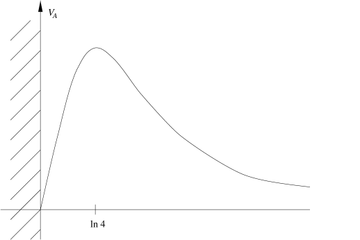
Figure 1. $V_{A}(\chi)$ for $R+\epsilon^{-2}R^{3}$ gravity

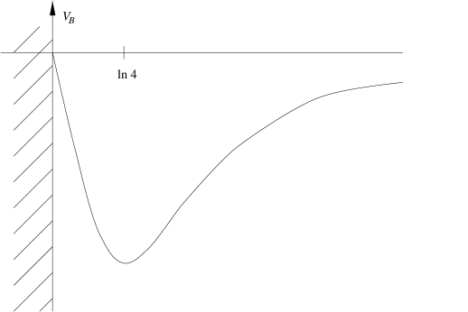
Figure 2. $V_{B}(\chi)$ for $R+\epsilon^{-2}R^{3}$ gravity

As a concrete example of all this, we return to the example specified in (2.3). As discussed previously, there are two branches where the second order theory is defined; branch A where $0<X<\infty$ and branch B where $-\infty<X<0$. The field $\lambda$, which is given as a function of $X$ in (2.5), satisfies $\lambda>1$ everywhere and, hence, $\chi=\log\lambda$ is well defined in both branches, although its range in restricted to $0<\chi<\infty$. Expression (2.5) was inverted to give $X$ as a function of $\lambda$ in (2.6). This expression is branch dependent, being given by $X=\pm(\epsilon/\sqrt{3})\sqrt{\lambda-1}$ with the positive root chosen in branch A and the negative root chosen in branch B. It follows that the form of the potential energy defined in (2.10) also depends on the branch chosen. It is given by

$$V_{A}(\chi) =+\frac{2}{9\sqrt{3}}\epsilon e^{-2\chi}(e^{\chi}-1)^{3/2}$$ (2.14)

$$V_{B}(\chi) =-\frac{2}{9\sqrt{3}}\epsilon e^{-2\chi}(e^{\chi}-1)^{3/2}$$

for branch A and B respectively. The two potentials are plotted in Figures 1 and 2. We see that each has a stationary point. However, since vacua must be minima of the potential, it follows that only branch B has a stable vacuum. This is located at $\chi=\ln 4$, which is non-zero. Note that $V_{B}(\ln 4)=-\epsilon/24$, so that the vacuum state has a non-vanishing negative cosmological constant. It follows that $\overline{R}=-\epsilon/4$ and $R=-\epsilon$, which implies that the vacuum state is an anti-de Sitter space both in terms of the metric $\overline{g}_{\mu\nu}$ and the metric $g_{\mu\nu}$. Thus we have given an example of a higher-derivative theory which has a new vacuum state away from the flat-space solution of ordinary Einstein gravity. It is important to note that none of this structure would have been evident if we had made a simple expansion of the original action around flat space in terms of $h_{\mu\nu}=g_{\mu\nu}-\eta_{\mu\nu}$. In fact, keeping only the first non-trivial, quadratic terms in $h_{\mu\nu}$, we would not even have been aware that there was an additional scalar degree of freedom in the theory. The lowest order term in $R^{3}$ is cubic in $h_{\mu\nu}$, and so in a quadratic expansion we would only see the usual Einstein term.

The conclusion is that generic higher-derivative corrections to pure Einstein gravity introduce completely new vacuum states into the theory. Flat space is no longer a unique point in field space, so that if, for instance, we wish to investigate the fundamental excitations in the theory, we must start by specifying which vacuum state we are considering.

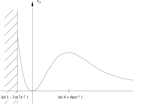
Figure 3. $V_{A}(\chi)$ for $R+3\alpha\epsilon^{-2}R^{2}+\epsilon^{-2}R^{3}$ gravity

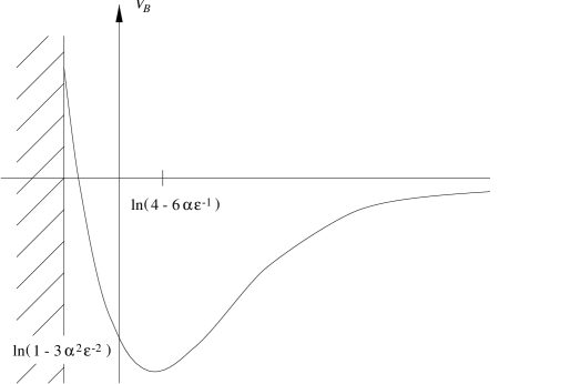
Figure 4. $V_{B}(\chi)$ for $R+3\alpha\epsilon^{-2}R^{2}+\epsilon^{-2}R^{3}$ gravity

At this point, we would like to present another specific example that further illustrates the preceding discussion. Consider the cubic function

$$f(R)=R+3\alpha\epsilon^{-2}R^{2}+\epsilon^{-2}R^{3}$$ (2.15)

with $\epsilon>\sqrt{3}\alpha>0$. We now have

$$f^{\prime\prime}(X)=6\epsilon^{-2}(X+\alpha)$$ (2.16)

so that the theory has a single critical point at $X=-\alpha$. It follows that the second-order theory is defined on two branches; branch A where $-\alpha<X<\infty$ and branch B where $-\infty<X<-\alpha$. On either branch we can define a new field $\lambda=f^{\prime}(X)$, which in this case is given by

$$\lambda=1+6\alpha\epsilon^{-2}X+3\epsilon^{-2}X^{2}.$$ (2.17)

Note that, since $\epsilon>\sqrt{3}\alpha$, $\lambda$ is always a positive real number in the range $1-3\alpha^{2}\epsilon^{-2}<\lambda<\infty$ for both branches. Expression (2.17) can be inverted to give

$$X_{\pm}=-\alpha\pm\sqrt{\alpha^{2}+\tfrac{1}{3}\epsilon^{2}(\lambda-1)}.$$ (2.18)

Clearly the $X_{+}$ solution is correct on branch A whereas the $X_{-}$ solution is to be used in branch B. Since $\lambda$ is always positive, the definition of $\chi=\ln\lambda$ is valid in both branches. Note that $\chi$ is then restricted to lie in the range $\ln(1-3\alpha^{2}\epsilon^{-2})<\chi<\infty$. Since the expression for $X$ in terms of $\lambda$, and hence $\chi$, given in (2.18) is different in each branch, it follows from (2.10) that the potential energy function also is different in each branch. We have

$$V_{A}(\chi) =\tfrac{1}{3}\epsilon^{-2}e^{-2\chi}\left(X_{+}(\chi)\right)^{2}\left(3\alpha+2X_{+}(\chi)\right),$$ (2.19)

$$V_{B}(\chi) =\tfrac{1}{3}\epsilon^{-2}e^{-2\chi}\left(X_{-}(\chi)\right)^{2}\left(3\alpha+2X_{-}(\chi)\right),$$

where

$$X_{\pm}(\chi)=-\alpha\pm\sqrt{\alpha^{2}+\tfrac{1}{3}\epsilon^{2}(e^{\chi}-1)}$$ (2.20)

and the $V_{A}$ expression is valid in branch A and the $V_{B}$ expression valid in branch B. The two potentials are plotted in Figures 3 and 4. Unlike the previous example, in this case each branch contains a single, stable minimum. In branch A, this minimum is located at $\chi=0$ and has vanishing cosmological constant $V(0)=0$. It follows that, for this vacuum, $\overline{R}=R=0$ and spacetime is flat with respect to both the $\overline{g}_{\mu\nu}$ and $g_{\mu\nu}$ metrics. In branch B, the minimum is located at $\chi=\ln(4-6\alpha\epsilon^{-1})$ with a non-vanishing negative cosmological constant given by $V(\chi)=-\epsilon^{2}/6(4\epsilon-6\alpha)$. For this vacuum $\overline{R}=-\epsilon^{2}/(4\epsilon-6\alpha)$ and, hence, $R=-\epsilon$. It follows that the spacetime is an anti de-Sitter space with respect to both metrics $\overline{g}_{\mu\nu}$ and $g_{\mu\nu}$. Thus we have found an example which, aside from a conventional minimum at $R=0$ with zero cosmological constant, has an additional minimum with negative cosmological constant. Furthermore, there is an unstable maximum with positive cosmological constant. The mass of the scalar field is different at each of the different minima. Here a quadratic expansion of the action around flat-space would have identified a new scalar degree of freedom, but would never have revealed the presence of a second stable vacuum state.

It will not have escaped the readers notice that finding the vacua in the second-order formalism requires a careful discussion of the branches in the $X$ variable. The branching structure was not too difficult in the preceding examples, but as we will show below, it can be, and generally is, extremely complicated. However, the following remarks will allow us to define a simpler procedure for determining the vacua. Recall that, for a covariantly constant scalar $\chi$ satisfying $dV/d\chi=0$, the corresponding spacetime structure in terms of the metric $g_{\mu\nu}$ is that of a space of constant curvature with $R=6e^{\chi}V(\chi)$. Provided we are not at a degenerate point, spaces of constant curvature $R$ and vacuum solutions are in one-to-one correspondence, since the relation $R=6e^{\chi}V(\chi)$ not only means that constant $\chi$ implies constant $R$, but also the reverse. Note that, as a corollary, any vacuum solution with zero cosmological constant, namely $V(\chi)=0$, must correspond to flat space in the original higher-derivative theory. An important consequence of this result is that, since flat space is a single point in the field space of the original theory, there can be only one vacuum state with zero cosmological constant in the second-order theory. We conclude that all vacuum solutions of the above type can be found as constant curvature solutions of the equations of motion for the higher-derivative $g_{\mu\nu}$ theory. All such vacua can be found directly, without reference to any branch structure. Having found a vacuum of interest, one can then proceed in reverse, introducing the second-order theory in the appropriate branch containing that vacuum. This is often an easier procedure. The $g_{\mu\nu}$ equations derived from the higher-derivative action (2.1) are

$$R_{\mu\nu}f^{\prime}(R)-\tfrac{1}{2}g_{\mu\nu}f(R)-\left(\nabla_{\mu}\nabla_{\nu}-g_{\mu\nu}\nabla^{2}\right)f^{\prime}(R)=0.$$ (2.21)

If we look for solutions of constant curvature, then $R_{\mu\nu}=\tfrac{1}{4}g_{\mu\nu}R$ where $R$ is a constant. It follows that the derivative terms in the equations of motion drop out and we are left with the simple condition, first derived by Barrow and Ottewill [10],

$$Rf^{\prime}(R)-2f(R)=0.$$ (2.22)

We see that this is exactly the condition we obtained for stationary points of the potential (2.13) aside from a factor of $e^{-2\chi}$. In the latter case, however, the expression was taken to be a function of the scalar field $\chi$ expressed in terms of $X$, and as such only valid in a branch-by-branch sense, whereas here the expression is valid for all curvature $R$.

This now provides us with a procedure for finding all the vacua of the theory as well as the nature of the excitations around a given vacuum. We start by looking for constant curvature solutions of the original higher-derivative equations of motion, solving the equation (2.22), which is valid globally. Having identified these points we can then, locally around each solution, make a transformation to the reduced theory, choosing, if necessary, the appropriate branch of $X(e^{\chi})$. In the transformed frame, the new scalar degree of freedom is made explicit. We can then address questions of local stability and the mass of the scalar field. The only breakdown of this procedure occurs when the minimum is at a degenerate point of the transformation; that is, a point where $f^{\prime\prime}(R)=0$. In this case, any discussion of the particle spectrum and local stability must be in terms of the original theory. In general, we shall not consider such degenerate points.

As an example of this procedure, consider the function

$$f(R)=\tfrac{1}{2}\left[R+\epsilon\sin\left(R/\epsilon\right)\right].$$ (2.23)

Where $\epsilon$ is a constant. The condition for a degenerate point is then

$$f^{\prime\prime}(R)=-\tfrac{1}{2}\epsilon^{-1}\sin\left(R/\epsilon\right)=0.$$ (2.24)

This equation has solutions $R=n\pi\epsilon$ where $n$ is any integer. The theory thus has an infinite number of branches given by $n\pi\epsilon<R<(n+1)\pi\epsilon$. Rather than treating each branch separately, we follow our procedure for finding the vacuum states of the theory by solving the condition (2.22) for the constant curvature solutions of the original theory. The condition reads

$$\sin\left(R/2\epsilon\right)\left[\left(R/2\epsilon\right)\sin\left(R/2\epsilon\right)-\cos\left(R/2\epsilon\right)\right]=0.$$ (2.25)

The left-hand side of this expression is plotted in figure 5. We have the solutions

$$R=2n\pi\epsilon,\;2\delta_{n}\epsilon$$ (2.26)

where $n$ is an integer and $\delta_{n}$ are the solutions of

$$\delta\sin\delta-\cos\delta=0.$$ (2.27)

Explicitly, the first few solutions of (2.27) near $\delta=0$ are

$$\dots,\;\delta_{-2}\approx-6.12,\;\delta_{-1}\approx-2.80,\;\delta_{1}\approx 2.80,\;\delta_{2}\approx 6.12,\;\dots$$ (2.28)

Furthermore $(\left|n\right|-\tfrac{1}{2})\pi<\left|\delta_{n}\right|<\left|n\right|\pi$ and as $\left|\delta\right|$ becomes large the solutions approach $\delta_{n}=n\pi$.

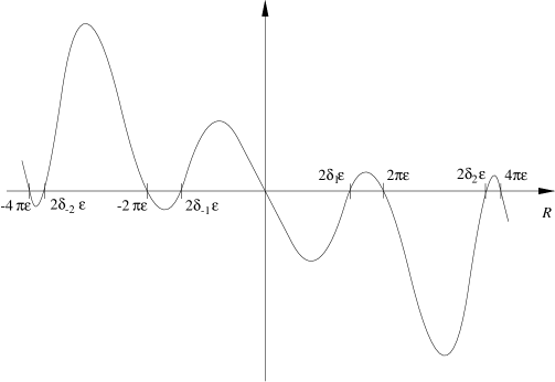
Figure 5. Condition for a constant curvature solution of $\tfrac{1}{2}\left[R+\epsilon\sin(R/\epsilon)\right]$ gravity

The first observation to make is that the constant curvature solutions at $R=2n\pi\epsilon$, including the point $R=0$, all correspond to degenerate points. As such, a second-order form of the theory does not exist at these points. Thus, although these are constant curvature solutions, we cannot identify them as vacuum solutions of a canonical second-order theory. However the solutions at $R=2\delta_{n}\epsilon$ are not at degenerate points. From our previous discussion this implies that they must correspond to vacuum solutions of the canonical second-order theory. Nonetheless, we find that each vacuum solution lies in a different branch of the theory.

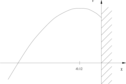
Figure 6. $V(\chi)$ for the branch $\pi\epsilon<R<2\pi\epsilon$

Let us consider two particular solutions, $R=2\delta_{1}\epsilon\approx 5.60\epsilon$ and $R=2\delta_{-1}\epsilon=-2\delta_{1}\epsilon\approx-5.60\epsilon$, in the second-order formulation. For the first solution we must take the branch $\pi\epsilon<R<2\pi\epsilon$. Following our usual procedure for writing the theory in a second-order form, we first introduce the auxiliary field $X$ and then define

$$\lambda=f^{\prime}(X)=\tfrac{1}{2}\left[1+\cos\left(X/\epsilon\right)\right].$$ (2.29)

However, as usual, we are required to invert this expression to give $X$ as a function of $\lambda$. It follows that

$$X=\epsilon\cos^{-1}\left(2\lambda-1\right)\qquad\text{with $\pi\epsilon<X<2\pi\epsilon$}.$$ (2.30)

We note that $\lambda$ is only defined in the range $0<\lambda<1$. To put the action in canonical second-order form we define $\chi=\ln\lambda$. The potential for $\chi$ (2.10), is then given by

$$V(\chi)=\tfrac{1}{3}e^{-2\chi}\left[X(\chi)\cos\left(X(\chi)/\epsilon\right)-\epsilon\sin\left(X(\chi)/\epsilon\right)\right]$$ (2.31)

where,

$$X(\chi)=\epsilon\cos^{-1}\left(2e^{\chi}-1\right)\qquad\text{with $\pi\epsilon<X<2\pi\epsilon$}.$$ (2.32)

We now have that $\chi$ is restricted to the range $-\infty<\chi<0$. The potential is plotted in figure 6. We find that there is a single maximum of the potential at $\chi\approx-0.12$. The value of the potential at this point is $V(\chi)\approx 1.05\epsilon$, so that $\overline{R}=6V(\chi)\approx 6.31\epsilon$ and $R=6e^{\chi}V(\chi)\approx 5.60\epsilon$. Thus we see that the maximum corresponds to the flat space solution $R=2\delta_{1}\epsilon$ as expected, and we can conclude that this vacuum is unstable.

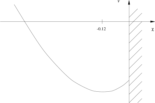
Figure 7. $V(\chi)$ for the branch $-2\pi\epsilon<R<-\pi\epsilon$

For the solution at $R=2\delta_{-1}\epsilon$, we must take the branch $-2\pi\epsilon<R<-\pi\epsilon$. The expression for the potential is the same as the expression (2.31) above, except that we must now define

$$X(\chi)=\epsilon\cos^{-1}\left(2e^{\chi}-1\right)\qquad\text{with $-2\pi\epsilon<X<-\pi\epsilon$}.$$ (2.33)

The resulting potential is plotted in figure 7. Again $\chi$ is restricted to lie in the range $-\infty<\chi<0$. We now find a stable minimum at $\chi\approx-0.12$. This gives $V(\chi)\approx-1.05\epsilon$, $\overline{R}=6V(\chi)\approx-6.31\epsilon$ and $R=6e^{\chi}V(\chi)\approx-5.60\epsilon$, showing that the minimum of the potential does indeed correspond to the constant curvature solution $R=2\delta_{-1}\epsilon$. We can concluded that this is a stable vacuum state. In fact, further analysis shows that all the vacua $R=2\delta_{n}\epsilon$ with $\delta_{n}>0$ are unstable maxima, while those with $\delta_{n}<0$ are stable minima. This final example demonstrates that the vacuum structure of higher-derivative theories can be complicated. We find an infinite number of stable and unstable vacua, each in a different branch of the theory.

In summary, we have shown that theories which are general functions of the scalar curvature $R$, can be reduced to a canonical second-order form describing Einstein gravity coupled to a scalar field with a potential which may have a vacuum structure of arbitrary complexity. Further these vacua all correspond to constant curvature solutions of the original theory. The advantage of discussing the theory in the second-order formalism is that it is in a canonical form where we can easily identify the excitations around the vacuum. The disadvantage is that the problem of inverting $f^{\prime}(X)$ means that we are forced to break the theory into regions separated by degenerate points. For this reason it is often easier to identify vacua as constant curvature solutions of the higher-derivative theory and then make a local transformation in the region of each solution to investigate the excitations around that vacuum. All of the non-trivial vacuum structure arises from non-linear terms in the field equations and so is missed in a quadratic expansion of the higher-derivative theory in terms of the fluctuation of the metric around flat space. Further, any analysis of the particle content of the theory, in this case the presence of a new scalar degree of freedom and identification of its mass, can only be made once the vacuum is identified.

3. Actions Given by General Functions of the Ricci Tensor

In this and the following section we shall extend our discussion to include actions which are general functions of first the Ricci tensor and then the Riemann tensor. We shall use the same techniques as in the previous section, namely introducing auxiliary fields, showing that vacuum states correspond to constant curvature solutions of the higher derivative theory, and then investigating the excitations around a given vacuum. The reduction to a second-order form was first discussed by Magnano et al. [3, 4, 5] and Jakubiec and Kijowski [6]. Here, we shall use a slightly different analysis, again pointing out the need for identifying different branches of the theory and also giving a canonical separation of the new variables about any given vacuum. We shall only give the general formulation without specific examples. Again we will find a rich structure of vacua which would be completely missed in a linearized analysis. This will re-emphasize the need to identify the vacuum in question before investigating the masses and couplings of the elementary excitations of the theory.

Starting with an action $f(R_{\mu\nu})$ we can introduce an auxiliary field and put the theory in a second-order form

$$S =\frac{1}{2\kappa^{2}}\int{d^{4}x\sqrt{-g}f(R_{\mu\nu})}$$

$$=\frac{1}{2\kappa^{2}}\int{d^{4}x\sqrt{-g}\left[\frac{df(X_{\rho\sigma})}{dX_{\mu\nu}}\left(R_{\mu\nu}-X_{\mu\nu}\right)+f(X_{\mu\nu})\right]}$$

$$=\frac{1}{2\kappa^{2}}\int{d^{4}x\sqrt{-g}\left[\pi^{\mu\nu}\left(R_{\mu\nu}-X_{\mu\nu}(\pi_{\rho\sigma})\right)+f(X_{\mu\nu}(\pi_{\rho\sigma}))\right]}.$$ (3.1)

Again we introduce the auxiliary field in two steps, first writing the action in terms of the field $X_{\mu\nu}$ which gets set to $R_{\mu\nu}$ on solving its equation of motion. We then define

$$\pi^{\mu\nu}=\frac{df(X_{\rho\sigma})}{dX_{\mu\nu}},$$ (3.2)

and invert the expression to give $X_{\mu\nu}$ as a function of $\pi_{\mu\nu}$. Note again that the introduction of both $X_{\mu\nu}$ and $\pi_{\mu\nu}$ requires the non-degeneracy condition

$$\det\frac{d^{2}f(X_{\kappa\lambda})}{dX_{\mu\nu}dX_{\rho\sigma}}\neq 0$$ (3.3)

if the auxiliary field is to be properly eliminated to return to the original action. Furthermore, in inverting (3.2), it may be necessary to divide the theory into branches corresponding to different possible roots for $X_{\mu\nu}$. Thus for the variable $\pi_{\mu\nu}$ it may be necessary to introduce a collection of auxiliary variable theories each valid for a different branch of $R_{\mu\nu}$.

We can ask how many degrees of freedom are there in the auxiliary field? We have argued that we expect six. If we consider the $X_{\mu\nu}$ formulation for now, we see first that we can again derive a spin-two divergence condition. Since the auxiliary field equation of motion gives $X_{\mu\nu}=R_{\mu\nu}$, we clearly can show, using the Bianchi identity $\nabla^{\mu}G_{\mu\nu}=0$, that $\nabla^{\mu}\left(X_{\mu\nu}-\tfrac{1}{2}g_{\mu\nu}X\right)=0$. Constraining the components of $X_{\mu\nu}$, these four conditions imply that we do indeed have six new propagating degrees of freedom. We would like to be able to separate these into scalar and spin-two degrees of freedom as was done in the quadratic case in [1]. For a general function $f$, this is not possible since we are not able to obtain the necessary trace condition from the $g_{\mu\nu}$ equation of motion. However, as we will show below, having identified a vacuum state, we can always make the separation locally in an expansion around the vacuum solution.

What then are the vacua of the $f(R_{\mu\nu})$ theory? Since we are unable to separate the spin-two and scalar degrees of freedom in the auxiliary field, we cannot put the theory in a canonical form and look to minimize the potential as we did for the $f(R)$ theory. However, we recall that the vacuum states in question are none other than states where the auxiliary field is covariantly constant. This means, since the $X_{\mu\nu}$ equation of motion gives $X_{\mu\nu}=R_{\mu\nu}$ that they are states of constant tensor curvature. We can also impose the condition that the states should have no preferred direction, so that $X_{\mu\nu}$ is proportional to the metric $g_{\mu\nu}$. Thus vacuum states are states of constant scalar curvature $R_{\mu\nu}=\tfrac{1}{4}Rg_{\mu\nu}$ with $R$ constant. Consequently, one approach to finding vacuum solutions is simply to look for constant curvature solutions of the original theory.

The equations of motion of the original higher derivative theory are given by

$$\nabla^{2}f^{\prime}_{\mu\nu}+g_{\mu\nu}\nabla^{\rho}\nabla^{\sigma}f^{\prime}_{\rho\sigma}-\nabla_{\rho}\nabla_{\mu}{f^{\prime}_{\nu}}^{\rho}-\nabla_{\rho}\nabla_{\nu}{f^{\prime}_{\mu}}^{\rho}+R_{\rho\mu}{f^{\prime}_{\nu}}^{\rho}+R_{\rho\nu}{f^{\prime}_{\mu}}^{\rho}-g_{\mu\nu}f=0.$$ (3.4)

To incorporate the presence of the metric in $f(R_{\mu\nu})$ in deriving the equations of motion, we consider $f$ as a function of the mixed index object ${R_{\mu}}^{\nu}$, with all contractions made between raised and lowered indices so that the metric does not enter explicitly. Then in the above expression ${f^{\prime}_{\mu}}^{\nu}=df/d{R_{\nu}}^{\mu}$, so that, for instance, $f^{\prime}_{\mu\nu}={f^{\prime}_{\mu}}^{\lambda}g_{\lambda\nu}$. Looking for constant curvature solutions of the form $R_{\mu\nu}=\tfrac{1}{4}g_{\mu\nu}R$, we obtain the condition

$$Rg^{\prime}(R)-2g(R)=0,$$ (3.5)

where $g(R)=f(\tfrac{1}{4}R{\delta_{\mu}}^{\nu})$ and $g^{\prime}(R)=dg(R)/dR$, and we have used the fact that ${f^{\prime}_{\mu}}^{\nu}$ evaluated at the constant curvature solution must be proportional to ${\delta_{\mu}}^{\nu}$. Note that this condition has exactly the same form as the condition (2.22) we obtained for actions which were general functions of the scalar curvature.

Given a particular vacuum solution satisfying the condition (3.5), we would like to investigate the excitations around the vacuum state. The natural way to do this is to consider an expansion of the action around a given vacuum $R=R_{0}$. Expanding $f(R_{\mu\nu})$ and keeping terms to quadratic order in the curvature only, we have

$$S =\frac{1}{2\kappa^{2}}\int{d^{4}x\sqrt{-g}\left[a_{0}+a_{1}\left(R-R_{0}\right)+\tfrac{1}{2}a_{2,1}\left(R-R_{0}\right)^{2}\right.}$$

$${\left.\hskip 108.405pt+\tfrac{1}{2}a_{2,2}\left(R_{\mu\nu}-\tfrac{1}{4}g_{\mu\nu}R_{0}\right)\left(R^{\mu\nu}-\tfrac{1}{4}g^{\mu\nu}R_{0}\right)\right]}$$

$$=\frac{\beta}{2\kappa^{2}}\int{d^{4}x\sqrt{-g}\left[-\tfrac{1}{2}R_{0}+R+\frac{1}{6{m_{0}}^{2}}R^{2}-\frac{1}{{m_{2}}^{2}}\left(R_{\mu\nu}R^{\mu\nu}-\tfrac{1}{3}R^{2}\right)\right]},$$ (3.6)

Here we have evaluated $f$ and its derivative at the vacuum $R_{\mu\nu}=\tfrac{1}{4}g_{\mu\nu}R_{0}$ and defined

$$\left.f\right|_{R_{0}} =a_{0},$$ (3.7)

$$\left.\frac{df}{dR_{\mu\nu}}\right|_{R_{0}} =a_{1}g^{\mu\nu},$$

$$\left.\frac{d^{2}f}{dR_{\mu\nu}dR_{\rho\sigma}}\right|_{R_{0}} =a_{2,1}g^{\mu\nu}g^{\rho\sigma}+\tfrac{1}{2}a_{2,2}\left(g^{\mu\rho}g^{\nu\sigma}+g^{\nu\rho}g^{\mu\sigma}\right),$$

using the general symmetric decomposition of the second two expressions. The variables $\beta$, $m_{0}$ and $m_{2}$ are then given by

$$\beta =a_{1}-\left(a_{2,1}+\tfrac{1}{4}a_{2,2}\right)R_{0},$$ (3.8)

$${m_{0}}^{2} =\frac{\beta}{3a_{2,1}+a_{2,2}},$$

$${m_{2}}^{2} =-\frac{2\beta}{a_{2,2}},$$

where in writing the final line of (3.6) we have used the constant curvature condition $a_{1}R_{0}=2a_{0}$. We see that we have succeeded in putting the action in a quadratic form, though with the addition of a cosmological constant.

The final line of (3.6) is identical to the general quadratic form we discussed in our previous paper [1], except for the addition of a cosmological constant term and a renormalization of the gravitational coupling constant by a factor $\beta$. We can thus introduce auxiliary fields $\chi$ and $\tilde{\pi}_{\mu\nu}$ exactly as we did in [1] to give

$$S=\frac{\beta}{2\kappa^{2}}\int{d^{4}x\sqrt{-\tilde{g}}}\left[\tilde{R}-\tfrac{3}{2}\left(\tilde{\nabla}\chi\right)^{2}-\tfrac{3}{2}{m_{0}}^{2}\left(1-e^{-\chi}\right)^{2}-\tfrac{1}{2}R_{0}e^{-2\chi}\right.\\ \left.-\tilde{G}_{\mu\nu}\tilde{\pi}^{\mu\nu}+\tfrac{1}{4}{m_{2}}^{2}\left(\tilde{\pi}_{\mu\nu}\tilde{\pi}^{\mu\nu}-\tilde{\pi}^{2}\right)\right].$$ (3.9)

The only effect of the cosmological term is to modify the potential for the scalar field, adding a term $\tfrac{1}{2}R_{0}e^{-2\chi}$. We find that the extremum of the potential is now at $3{m_{0}}^{2}\left(e^{\chi}-1\right)=R_{0}$, which, relating the auxiliary field $\chi$ back to the original curvature, gives $R=R_{0}$, as required for a consistent expansion. Following exactly the analysis of our previous paper, the auxiliary field $\tilde{\pi}_{\mu\nu}$ satisfies generalized divergence and trace conditions, so it does indeed describe the degrees of freedom of a spin-two field. By making a final field redefinition, we can write the action in canonical form with explicit kinetic energy terms for the spin-two field. Again following the discussion in our previous paper, the spin-two field will have the correct Pauli-Fierz limit, but will unfortunately be ghost-like.

Thus we have shown that locally, around any vacuum of the higher-derivative theory (that is a solution of constant curvature), we can expand the theory to identify a new scalar and a new spin-two degree of freedom (provided we are not at a degenerate point). The spin-two field satisfies divergence and trace conditions as before but importantly, we see that it remains ghost-like. Thus generalizing to $f(R_{\mu\nu})$ actions fails to remove the problem of the ghost spin-two degree of freedom. The masses of the degrees of freedom are fixed by the form of the function $f$ around the constant curvature solution.

It is worth noting that we could equally well have done this analysis in the second-order form, looking for solutions with constant $X_{\mu\nu}$ proportional to $g_{\mu\nu}$. Then expanding in small $X_{\mu\nu}$ about such solutions, gives a linear coupling between $X_{\mu\nu}$ and $R_{\mu\nu}$ and quadratic ‘mass’ terms for $X_{\mu\nu}$. From this form we could then extract the scalar and spin-two parts of $X_{\mu\nu}$. In this sense, the auxiliary field $X_{\mu\nu}$ always carries six degrees of freedom, which about any given vacuum can be decomposed into a scalar field and a ghost spin-two field, with the form of the decomposition changing as we go from vacuum to vacuum.

4. Actions Given by General Functions of the Riemann Tensor

Our last generalization is to consider actions which are general functions of the Riemann tensor $R_{\lambda\mu\nu\rho}$. As mentioned earlier, the suggestion is that such theories have an additional six degrees of freedom, which we know in the quadratic case can be decomposed into scalar and spin-two fields.

We start the discussion by demonstrating that, as in all previous cases, we can introduce an auxiliary field to write the action in a second order form.

$$S =\frac{1}{2\kappa^{2}}\int{d^{4}x\sqrt{-g}f(R_{\lambda\mu\nu\rho})}$$

$$=\frac{1}{2\kappa^{2}}\int{d^{4}x\sqrt{-g}\left[\frac{df(X_{\alpha\beta\gamma\delta})}{dX_{\lambda\mu\nu\rho}}\left(R_{\lambda\mu\nu\rho}-X_{\lambda\mu\nu\rho}\right)+f(X_{\lambda\mu\nu\rho})\right]}$$

$$=\frac{1}{2\kappa^{2}}\int{d^{4}x\sqrt{-g}\left[\rho^{\lambda\mu\nu\rho}\left(R_{\lambda\mu\nu\rho}-X_{\lambda\mu\nu\rho}(\rho_{\alpha\beta\gamma\delta})\right)+f(X_{\lambda\mu\nu\rho}(\rho_{\alpha\beta\gamma\delta}))\right]}.$$ (4.1)

Again we introduce the auxiliary field in two stages; first introducing $X_{\lambda\mu\nu\rho}$, which gets set equal to the Riemann tensor on solving its equation of motion, and then defining

$$\rho^{\lambda\mu\nu\rho}=\frac{df(X_{\alpha\beta\gamma\delta})}{dX_{\lambda\mu\nu\rho}}$$ (4.2)

In both cases we require the non-degeneracy condition

$$\det\frac{d^{2}f(X_{\alpha\beta\gamma\delta})}{dX_{\eta\kappa\lambda\mu}dX_{\nu\rho\sigma\tau}}=0,$$ (4.3)

in order to be able to eliminate the auxiliary field and return to the original action. When using the variable $\rho_{\lambda\mu\nu\rho}$ we may be required to break the theory into branches, introducing a collection of second-order theories, each taking a different branch when inverting to find $X_{\lambda\mu\nu\sigma}$ in terms of $\rho_{\lambda\mu\nu\rho}$.

Turning to the vacuum states, we again find that states with constant $X_{\lambda\mu\nu\sigma}$ have constant Riemann curvature, since $X_{\lambda\mu\nu\sigma}$ is set equal to $R_{\lambda\mu\nu\sigma}$ by its equation of motion. Furthermore, imposing the condition that there is no preferred direction in spacetime we require that $X_{\lambda\mu\nu\sigma}$ is proportional to $g_{\mu\nu}$. Therefore, given the symmetries of $X_{\lambda\mu\nu\sigma}$, we have

$$R_{\lambda\mu\nu\sigma}=R^{0}_{\lambda\mu\nu\sigma}=\tfrac{1}{12}R_{0}\left(g_{\lambda\nu}g_{\mu\sigma}-g_{\lambda\sigma}g_{\mu\nu}\right),$$ (4.4)

and, hence, we are considering solutions of constant Ricci scalar curvature.

As before the easiest way to obtain such solutions is from the equations of motion of the original higher-derivative action. Again, to circumvent the problem, when deriving the equation of motion, of the metric explicitly entering the function $f$, we consider $f$ as a function of $R_{\mu\;\>\nu}^{\;\;\rho\;\>\sigma}$ with all contractions made between raised and lowered indices. We then derive the equations of motion

$$\nabla^{\rho}\nabla^{\sigma}f^{\prime}_{\mu\rho\nu\sigma}+\nabla^{\rho}\nabla^{\sigma}f^{\prime}_{\nu\rho\mu\sigma}+\tfrac{1}{2}{R_{\mu}}^{\rho\sigma\tau}f^{\prime}_{\nu\rho\sigma\tau}+\tfrac{1}{2}{R_{\nu}}^{\rho\sigma\tau}f^{\prime}_{\mu\rho\sigma\tau}-\tfrac{1}{2}g_{\mu\nu}f=0,$$ (4.5)

where ${f^{\prime}}_{\mu\;\>\nu}^{\;\;\rho\;\>\sigma}=df/dR_{\rho\;\>\sigma}^{\;\;\mu\;\>\nu}$. Restricting to constant curvature solutions of the form (4.4), we get the familiar condition

$$R_{0}g^{\prime}(R_{0})-2g(R_{0})=0,$$ (4.6)

where now $g(R_{0})=f(R^{0}_{\lambda\mu\nu\rho})$ and $g^{\prime}(R_{0})=dg(R_{0})/dR_{0}$, and we have used the fact that, by symmetry, ${f^{\prime}}_{\mu\;\>\nu}^{\;\;\rho\;\>\sigma}(R^{0}_{\lambda\mu\nu\rho})$ is proportional to ${\delta_{\mu}}^{\rho}{\delta_{\nu}}^{\sigma}-g_{\mu\nu}g^{\rho\sigma}$.

To investigate the excitations around a given vacuum we expanding the action about the constant curvature solution. We have, keeping terms up to quadratic order in the curvature only,

$$S =\frac{1}{2\kappa^{2}}\int{d^{4}x\sqrt{-g}\left[a_{0}+a_{1}\left(R-R_{0}\right)\right.}$$

$$\qquad\qquad\left.+\tfrac{1}{2}a_{2,1}\left(R-R_{0}\right)^{2}+\tfrac{1}{2}a_{2,2}\left(R_{\mu\nu}-\tfrac{1}{4}g_{\mu\nu}R_{0}\right)\left(R^{\mu\nu}-\tfrac{1}{4}g^{\mu\nu}R_{0}\right)\right.$$

$$\qquad\qquad\left.+\tfrac{1}{2}a_{2,3}\left(R_{\lambda\mu\nu\rho}-\tfrac{1}{12}R_{0}\left[g_{\lambda\nu}g_{\mu\rho}-g_{\lambda\rho}g_{\mu\nu}\right]\right)\left(R^{\lambda\mu\nu\rho}-\tfrac{1}{12}R_{0}\left[g^{\lambda\nu}g^{\mu\rho}-g^{\lambda\rho}g^{\mu\nu}\right]\right)\right]$$

$$=\frac{\beta}{2\kappa^{2}}\int{d^{4}x\sqrt{-g}\left[-\tfrac{1}{2}R_{0}+R+\frac{1}{6{m_{0}}^{2}}R^{2}-\frac{1}{{m_{2}}^{2}}\left(R_{\mu\nu}R^{\mu\nu}-\tfrac{1}{3}R^{2}\right)\right.}$$

$$\qquad\qquad\left.+\gamma\left(R_{\lambda\mu\nu\rho}R^{\lambda\mu\nu\rho}-4R_{\mu\nu}R^{\mu\nu}+R^{2}\right)\right].$$ (4.7)

Here we evaluate $f$ and its derivatives at the constant curvature solution, defining, for the contraction of the derivatives with a tensor $\Delta_{\lambda\mu\nu\rho}$ which has the symmetries of the Riemann tensor but in otherwise arbitrary,

$$\left.f\right|_{R_{0}} =a_{0},$$ (4.8)

$$\left.\frac{df}{dR_{\lambda\mu\nu\rho}}\right|_{R_{0}}\Delta_{\lambda\mu\nu\rho} =a_{1}\Delta,$$

$$\left.\frac{d^{2}f}{dR_{\eta\kappa\lambda\mu}dR_{\nu\rho\sigma\tau}}\right|_{R_{0}}\Delta_{\eta\kappa\lambda\mu}\Delta_{\nu\rho\sigma\tau} =a_{2,1}\Delta^{2}+a_{2,2}\Delta_{\mu\nu}\Delta^{\mu\nu}+a_{2,3}\Delta_{\lambda\mu\nu\rho}\Delta^{\lambda\mu\nu\rho},$$

with $\Delta_{\mu\nu}=g^{\lambda\rho}\Delta_{\mu\lambda\nu\rho}$ and $\Delta=g^{\mu\nu}\Delta_{\mu\nu}$. We have also introduced the parameters

$$\begin{aligned} \beta&=a_{1}-\left(a_{2,1}+\tfrac{1}{4}a_{2,2}+\frac{1}{6}a_{2,3}\right)R_{0},\\ {m_{0}}^{2}&=\frac{\beta}{3a_{2,1}+a_{2,2}+a_{2,3}},\end{aligned}\qquad\begin{aligned} \gamma=\frac{a_{2,3}}{2\beta},\\ {m_{2}}^{2}=-\frac{2\beta}{a_{2,2}+4a_{2,3}},\end{aligned}$$ (4.9)

and have used the constant curvature condition $a_{1}R_{0}=2a_{0}$ in the final line of (4.7).

The final expression in (4.7) is a quadratic action with a Gauss-Bonnet term, a Weyl-squared term and a Ricci-scalar-squared term, together with a cosmological constant. The Gauss-Bonnet term can be dropped classically as a total divergence, leaving the action in the same quadratic form as discussed in our previous paper [1]. Reducing the action to a second-order form then follows exactly as in the case for $f(R_{\mu\nu})$ actions, so that we obtain the same transformed action (3.9). Again we can verify that the transformed action has a vacuum solution at $R=R_{0}$ as is required for the consistency of our expansion. We also note that here too the expansion could have been made in terms of the variable $X_{\lambda\mu\nu\rho}$, which could then be decomposed into its scalar and spin-two parts, the form of the decomposition depending on which vacuum is being considered.

In conclusion, general actions of the form $f(R_{\lambda\mu\nu\rho})$ may have a variety of vacuum solutions, generically not apparent in a linear analysis. Around any vacuum the new degrees of freedom in the theory, aside from the massless graviton, can always be separated into a scalar field and a spin-two field. Unfortunately, the spin-two field is always ghost-like.

5. Higher-order Actions

In this section, we shall briefly discuss how to extend our analysis to actions with higher-order equations of motion. We have seen that an action involving any function of the curvature tensors gives at most fourth-order equations of motion. For higher-order equations we need to consider actions which include some derivatives of the curvature. Here, we shall be concerned with only the simplest form,

$$S=\frac{1}{2\kappa^{2}}\int{d^{4}x\sqrt{-g}f(R,\nabla^{2}R,\nabla^{4}R,\ldots,\nabla^{2k}R)},$$ (5.1)

where we require that the function $f$ has been reduced, by integration by parts and dropping total derivatives, so as to minimize $k$. The equations of motion following from similar actions have been considered by Schmidt [8] and Wands [9], who showed them to be equivalent to those for a set of scalar fields coupled to gravity. Here will shall show the full equivalence in a new way, working at the level of the action .

It will be important to distinguish between possible forms of the function $f$. If we write $f=f(\lambda_{1},\lambda_{2},\ldots,\lambda_{k+1})$, (where in the action we have $\lambda_{1}=R$, $\lambda_{2}=\nabla^{2}R$ and so on), we find there are two possible cases: either $\partial f/\partial\lambda_{k+1}$ is a function of $\lambda_{k+1}$ (case one) or it is not (case two). If it is not then it must be a function of $\lambda_{k}$, since otherwise the original form was reducible; that is, the action was not written in a form minimized with respect to $k$. Thus, in case two, we can always decompose $f$ as

$$\text{case 2:}\qquad f(\lambda_{1},\lambda_{2},\ldots,\lambda_{k},\lambda_{k+1})=g(\lambda_{1},\lambda_{2},\ldots,\lambda_{k})\lambda_{k+1}+h(\lambda_{1},\lambda_{2},\ldots,\lambda_{k}).$$ (5.2)

Further, we see that for case one the equations of motion are $(4k+4)$th-order, while for case two they are $(4k+2)$th-order.

We would like to reduce the action (5.1) to a canonical second-order form, by introducing auxiliary fields. Given the order of the higher-derivative equations of motion we see that in case one we must introduce $2k+1$ new fields, while in case two we need only $2k$ new fields. The procedure we shall use is essentially a generalization of Ostrogradski’s method for reducing a higher-order action to a first-order form [12, 13], only that here we shall be reducing to a second-order form. (The Ostrogradski result is usual given as a Hamiltonian, but this can always be rewritten as a Helmhotz Lagrangian, the analog of the form we shall use.)

We start by introducing a set of Lagrange multipliers, so

$$S=\frac{1}{2\kappa^{2}}\int{d^{4}x}\sqrt{-g}\left[f(\lambda_{1},\lambda_{2},\ldots,\lambda_{k+1})+\mu\left(R-\lambda_{1}\right)\right.\\ \left.+\mu_{1}\left(\nabla^{2}\lambda_{1}-\lambda_{2}\right)+\cdots+\mu_{k}\left(\nabla^{2}\lambda_{k}-\lambda_{k+1}\right)\right].$$ (5.3)

Clearly eliminating fields via the Lagrange multiplier equations of motion, starting with $\mu_{k}$ and working down in $k$ returns one to the original action.

However, we have introduced at least one too many new fields. It is clear that the $\lambda_{k+1}$ equation of motion is purely algebraic and eliminating it will not introduce higher-derivatives; that is, the action will remain second order. The $\lambda_{k+1}$ equation of motion reads

$$\mu_{k}=\begin{cases}{\displaystyle\frac{\partial f}{\partial\lambda_{k+1}}(\lambda_{1},\lambda_{2},\ldots,\lambda_{k},\lambda_{k+1})}&\text{in case 1},\\ {\displaystyle g(\lambda_{1},\lambda_{2},\ldots,\lambda_{k})}&\text{in case 2},\end{cases}$$ (5.4)

where we have distinguished between the two cases discussed above, and substituted the special form of $f$ in case two. In case one, to form the analog of Ostrogradski’s Lagrangian, we solve the equation to give $\lambda_{k+1}$ as a function of $\lambda_{1},\dots,\lambda_{k}$ and $\mu_{k}$, writing $\lambda_{k+1}={\tilde{\lambda}}_{k+1}(\lambda_{1},\ldots,\lambda_{k},\mu_{k})$. It should be noted that in general the solution is not unique, and we must divide the original theory into pieces corresponding to different branches of the solution, just as in the case of actions of the form $f(R)$ discussed in the previous section. In case two we simply substitute for $\mu_{k}$ and the special form of $f$. We get in case one

$$\text{case 1:}\qquad S=\frac{1}{2\kappa^{2}}\int{d^{4}x}\sqrt{-g}\left[f(\lambda_{1},\lambda_{2},\ldots,\lambda_{k},{\tilde{\lambda}}_{k+1}(\lambda_{1},\ldots,\lambda_{k},\mu_{k}))+\mu\left(R-\lambda_{1}\right)\right.\\ \left.+\mu_{1}\left(\nabla^{2}\lambda_{1}-\lambda_{2}\right)+\cdots+\mu_{k}\left(\nabla^{2}\lambda_{k}-{\tilde{\lambda}}_{k+1}(\lambda_{1},\ldots,\lambda_{k},\mu_{k})\right)\right],$$ (5.5)

the exact analog of the Ostrogradski-Helmhotz Lagrangian, while for case two we have a slightly different form,

$$\text{case 2:}\qquad S=\frac{1}{2\kappa^{2}}\int{d^{4}x}\sqrt{-g}\left[h(\lambda_{1},\lambda_{2},\ldots,\lambda_{k})+\mu\left(R-\lambda_{1}\right)\right.\\ \left.+\mu_{1}\left(\nabla^{2}\lambda_{1}-\lambda_{2}\right)+\cdots+g(\lambda_{1},\lambda_{2},\ldots,\lambda_{k})\nabla^{2}\lambda_{k}\right].$$ (5.6)

We see that, as expected, in case one we have a total of $2k+1$ auxiliary fields, while in case two we have only $2k$ new fields.

All that remains is to transform the action into a canonical form, growing canonical kinetic energy terms for all the new auxiliary fields. Let us concentrate on actions of case one. Terms of the form $\mu_{i}\nabla^{2}\lambda_{i}$ are easy to deal with. Simply introducing a pair of new fields, $\chi_{i}$ and $\psi_{i}$ by

$$\lambda_{i}=\chi_{i}+\psi_{i},\qquad\mu_{i}=\chi_{i}-\psi_{i},$$ (5.7)

we have, in the action,

$$\int{d^{4}x\sqrt{-g}\mu_{i}\nabla^{2}\lambda_{i}} =\int{d^{4}x\sqrt{-g}\left[\chi_{i}\nabla^{2}\chi_{i}-\psi_{i}\nabla^{2}\psi_{i}\right]}$$

$$=\int{d^{4}x\sqrt{-g}\left[-\left(\nabla\chi_{i}\right)^{2}+\left(\nabla\psi_{i}\right)^{2}\right]}.$$ (5.8)

We see that the $\chi_{i}$ field has a canonical kinetic term, but the $\psi_{i}$ field has the wrong sign; it is a ghost. This is characteristic of higher- order theories. In reducing the theory to second-order the new fields always enter as a pair of a ghost-like field with a ordinary field. If we define a potential function,

$$V(\chi_{1},\ldots,\chi_{k};\psi_{1},\ldots,\psi_{k})=\mu\lambda_{1}+\mu_{1}\lambda_{2}+\cdots+\mu_{k-1}\lambda_{k}+\mu_{k}{\tilde{\lambda}}_{k+1}(\lambda_{1},\ldots,\lambda_{k},\mu_{k})\\ -f(\lambda_{1},\lambda_{2},\ldots,\lambda_{k},{\tilde{\lambda}}_{k+1}(\lambda_{1},\ldots,\lambda_{k},\mu_{k}))$$ (5.9)

where it is understood that the right-hand side is evaluated at $\lambda_{i}=\chi_{i}+\psi_{i}$, $\mu_{i}=\chi_{i}-\psi_{i}$, the action in case one becomes

$$\text{case 1:}\qquad S=\frac{1}{2\kappa^{2}}\int{d^{4}x\sqrt{-g}\left[\mu R-\sum_{i}\left\{\left(\nabla\chi_{i}\right)^{2}-\left(\nabla\psi_{i}\right)^{2}\right\}-V(\chi_{1},\ldots,\chi_{k};\psi_{1},\ldots,\psi_{k})\right]}.$$ (5.10)

To complete the transformation to canonical form all that is left is to make a conformal rescaling of the metric to remove the $\mu R$ coupling. As usual we define $\chi=\log\mu$ and rescale to a metric $\overline{g}_{\mu\nu}=e^{\chi}g_{\mu\nu}$, giving

$$\text{case 1:}\qquad S=\frac{1}{2\kappa^{2}}\int{d^{4}x}\sqrt{-\overline{g}}\left[\overline{R}-\tfrac{3}{2}\left(\overline{\nabla}\chi\right)^{2}-e^{-\chi}\sum_{i}\left\{\left(\overline{\nabla}\chi_{i}\right)^{2}-\left(\overline{\nabla}\psi_{i}\right)^{2}\right\}\right.\\ \left.-e^{-2\chi}V(\chi_{1},\ldots,\chi_{k};\psi_{1},\ldots,\psi_{k})\right].$$ (5.11)

We conclude that the original case one higher-derivative gravity theory is equivalent to canonical Einstein gravity coupled to $2k+1$ scalar fields, $k+1$ of which, $\chi$ and $\chi_{i}$, propagate physically and $k$ of which, $\psi_{i}$, are ghost-like.

To put the case two action in canonical form is more complicated because of the $g(\lambda_{1},\lambda_{2},\ldots,\lambda_{k})\nabla^{2}\lambda_{k}$ term. However, in principle, it is always possible to introduce a set of new fields $\{\chi_{1},\ldots,\chi_{k};\psi_{1},\ldots,\psi_{k}\}$ which simultaneously diagonalize the kinetic terms for the $\lambda_{i}$ and $\mu_{i}$, though now the form of the transformation will depend on the function $g$. At least $k-1$ of the new fields will be ghost-like. We can then make a conformal rescaling as in case one to put the action in the same canonical form (5.11), though the potential function will have a different form.

The conclusion is that there is a procedure for rewriting the higher-order action (5.1) in a canonical second-order form. However, $k$ of the new fields in case one and at least $k-1$ of the fields in case two will be ghost-like. In each case we obtain a specific potential, and so we can again look for vacuum states as stationary points of the potential. Generically, as in the case of $f(R)$ actions discussed in the previous section, the non-trivial vacua do not correspond to the flat-space solution of the original higher-derivative theory.

As an simple example of this procedure consider the function $f=R+\alpha\left(\nabla^{2}R\right)^{2}$. This example is of the first case since writing $f(\lambda_{1},\lambda_{2})=\lambda_{1}+\alpha{\lambda_{2}}^{2}$ with $\lambda_{1}=R$ and $\lambda_{2}=\nabla^{2}R$, we have $\partial f/\partial\lambda_{2}=2\alpha\lambda_{2}$, which is not independent of $\lambda_{2}$. Following our general procedure, the first step is to introduce a set of Lagrange multipliers,

$$S =\frac{1}{2\kappa^{2}}\int{d^{4}x\sqrt{-g}\left[R+\alpha\left(\nabla^{2}R\right)^{2}\right]}$$

$$=\frac{1}{2\kappa^{2}}\int{d^{4}x\sqrt{-g}\left[\lambda_{1}+\alpha{\lambda_{2}}^{2}+\mu\left(R-\lambda_{1}\right)+\mu_{1}\left(\nabla^{2}\lambda_{1}-\lambda_{2}\right)\right]}.$$ (5.12)

As discussed above we have introduced one too many auxiliary fields. We can eliminate $\lambda_{2}$ by solving its equation of motion, which reads

$$2\alpha\lambda_{2}-\mu_{1}=0$$ (5.13)

implying $\lambda_{2}=\mu_{1}/2\alpha$. Substituting back into the action gives

$$S=\frac{1}{2\kappa^{2}}\int{d^{4}x\sqrt{-g}\left[\mu R+\mu_{1}\nabla^{2}\lambda_{1}+\lambda_{1}-\mu\lambda_{1}-\tfrac{1}{4}\alpha{\mu_{1}}^{2}\right]}.$$ (5.14)

Next, to put the kinetic energy for $\lambda_{1}$ and $\mu_{1}$ in canonical form, we define $\lambda_{1}=\chi_{1}+\psi_{1}$ and $\mu_{1}=\chi_{1}-\psi_{1}$, so that

$$S=\frac{1}{2\kappa^{2}}\int{d^{4}x\sqrt{-g}\left[\mu R-\left(\nabla\chi_{1}\right)^{2}+\left(\nabla\psi_{1}\right)^{2}-\left(\mu-1\right)\left(\chi_{1}+\psi_{1}\right)-\tfrac{1}{4}\alpha\left(\chi_{1}-\psi_{1}\right)^{2}\right]}.$$ (5.15)

Finally we make the conformal rescaling $\overline{g}_{\mu\nu}=e^{\chi}g_{\mu\nu}$ with $\chi=\log\mu$ to put the action in canonical form

$$S=\frac{1}{2\kappa^{2}}\int{d^{4}x}\sqrt{-\overline{g}}\left[\overline{R}-\tfrac{3}{2}\left(\overline{\nabla}\chi\right)^{2}-e^{-\chi}\left(\overline{\nabla}\chi_{1}\right)^{2}+e^{-\chi}\left(\overline{\nabla}\psi_{1}\right)^{2}\right.\\ \left.-e^{-2\chi}\left\{\left(e^{\chi}-1\right)\left(\chi_{1}+\psi_{1}\right)+\tfrac{1}{4}\alpha\left(\chi_{1}-\psi_{1}\right)^{2}\right\}\right].$$ (5.16)

Thus we see that the original higher-derivative gravity theory is equivalent to canonical Einstein gravity coupled to three scalar fields. One field is ghost-like, and the potential has a single, unstable stationary point at $\chi=\chi_{1}=\psi_{1}=0$.

As a second example consider $f=\alpha+\beta R+\gamma R^{2}+\epsilon R\nabla^{2}R$ Writing $\lambda_{1}=R$ and $\lambda_{2}=\nabla^{2}R$, we now have $\partial f/\partial\lambda_{2}=\epsilon\lambda_{1}$, independent of $\lambda_{2}$, so this example clearly falls under case two. Repeating our procedure, we introduce Lagrange multipliers to give

$$S =\frac{1}{2\kappa^{2}}\int{d^{4}x\sqrt{-g}\left[\alpha+\beta R+\gamma R^{2}+\epsilon R\nabla^{2}R\right]}$$

$$=\frac{1}{2\kappa^{2}}\int{d^{4}x\sqrt{-g}\left[\alpha+\beta\lambda_{1}+\gamma{\lambda_{1}}^{2}+\epsilon\lambda_{1}\lambda_{2}+\mu\left(R-\lambda_{1}\right)+\mu_{1}\left(\nabla^{2}\lambda_{1}-\lambda_{2}\right)\right]}.$$ (5.17)

Again we have too many new fields. The $\lambda_{2}$ equation of motion now reads

$$\epsilon\lambda_{1}=\mu_{1},$$ (5.18)

which cannot be solved for $\lambda_{2}$ since the action is case two. However substituting this solution into the action eliminates both $\lambda_{2}$ and $\mu_{1}$, leaving the second-order form,

$$S=\frac{1}{2\kappa^{2}}\int{d^{4}x\sqrt{-g}\left[\mu R-\epsilon\ (\nabla\lambda_{1})^{2}-\mu\lambda_{1}+\alpha+\beta\lambda_{1}+\gamma{\lambda_{1}}^{2}\right]}.$$ (5.19)

The kinetic energy for $\lambda_{1}$ is already in canonical form, but we must make a final conformal rescaling by $e^{\chi}=\mu$ to put the action in the completely canonical form

$$S=\frac{1}{2\kappa^{2}}\int{d^{4}x\sqrt{-\overline{g}}\left[\overline{R}-\tfrac{3}{2}\left(\overline{\nabla}\chi\right)^{2}-\epsilon e^{-\chi}\left(\overline{\nabla}\lambda_{1}\right)^{2}-V(\lambda_{1},\chi)\right]},$$ (5.20)

where we have the potential,

$$V(\lambda_{1},\chi)=e^{-2\chi}\left(e^{\chi}\lambda_{1}-\alpha-\beta\lambda_{1}-\gamma{\lambda_{1}}^{2}\right)$$ (5.21)

Again the original higher-derivative gravity is shown to be equivalent to ordinary Einstein gravity though now coupled to only two scalar fields. By choosing $\epsilon>0$ we can ensure that neither field is ghost-like. Note that we argued above that case two theories must have at least $k-1$ ghost-like fields. It is thus only in this special case of $k=1$ that we are able to have all the scalar fields non-ghost-like.

As before we obtain a specific potential for the fields. We find that $V(\lambda_{1},\chi)$ has a single stationary point at $\lambda_{1}=-2\alpha/\beta$, $\chi=\ln(\beta-4\alpha\gamma/\beta)$, provided $\beta-4\alpha\gamma/\beta>0$. Expanding around this point we find that, if $\alpha<0$ and $\beta<0$, we have a stable minimum. The value of the potential at the minimum is $V(\lambda_{1},\chi)=-\alpha/\left(\beta^{2}-4\alpha\gamma\right)$ which is negative. We conclude that, for the given range of $\alpha$, $\beta$ and $\gamma$, the theory has a single stable vacuum state with negative cosmological constant. From Einstein’s equation we find that this state is an anti-deSitter space with $\overline{R}=-2\alpha/\left(\beta^{2}-4\alpha\gamma\right)$. Using the fact that $R=e^{\chi}\overline{R}$ for covariantly constant $\chi$, we find that $R=-2\alpha/\beta$. Thus the vacuum state also corresponds to an anti-deSitter space in the original higher-derivative theory.

6. Conclusion

The most important conclusion of this paper is that higher-derivative theories of gravitation generically have multiple stable vacua. One of these may be trivial, corresponding to flat spacetime, but all the other vacua are non-trivial with the associated manifold being either deSitter or anti-deSitter spacetime with non-vanishing cosmological constant. While of interest from various points of view, such non-trivial vacua cannot represent the universe as it is now since the radius of curvature of these solutions is of order the inverse Planck mass. Thus, one might conclude that non-trivial gravitational vacua are irrelevant for particle physics theories. However, this is not the case. We have recently shown that if we extend the methods and results of this paper to the realm of $N=1$ supergravity, then non-trivial vacua can exist with vanishing cosmological constant [14]. Furthermore, we find that supersymmetry is generically spontaneously broken in these vacuum states. It follows that higher-derivative $N=1$ supergravitation could play a pivotal role in high energy physics. This possibility is being pursued elsewhere [15].

References

- [1] A. Hindawi, B. A. Ovrut, and D. Waldram, Consistent spin-two coupling and quadratic gravitation, Phys. Rev. D 53 (1996), 5583–5596, hep-th/9509142.
- [2] P. Teyssandier and Ph. Tourrenc, The Cauchy problem for the theories of gravity without torsion, J. Math. Phys. 24 (1983), 2793–2799.
- [3] G. Magnano, M. Ferraris, and M. Francaviglia, Nonlinear gravitational Lagrangians, Gen. Rel. Grav. 19 (1987), 465–479.
- [4] M. Ferraris, M. Francaviglia, and G. Magnano, Do nonlinear metric theories of gravitation really exist?, Class. Quantum Grav. 5 (1988), L95–L99.
- [5] G. Magnano, M. Ferraris, and M. Francaviglia, Legendre transformation and dynamical structure of higher-derivative gravity, Class. Quantum Grav. 7 (1990), 557–570.
- [6] A. Jakubiec and J. Kijowski, On theories of gravitation with nonlinear Lagrangians, Phys. Rev. D 37 (1988), 1406–1409.
- [7] S. Gottlöber, H.-J. Schmidt, and A. A. Starobinsky, Sixth-order gravity and conformal transformations, Class. Quantum Grav. 7 (1990), 893–900.
- [8] H.-J. Schmidt, Variational derivatives of arbitrarily high order and multi-inflation cosmological models, Class. Quantum Grav. 7 (1990), 1023–1031.
- [9] D. Wands, Extended gravity theories and the Einstein-Hilbert action, Class. Quantum Grav. 11 (1994), 269–279.
- [10] J. D. Barrow and A. C. Ottewill, The stability of general relativistic cosmological theory, J. Phys. A 16 (1983), 2757–2776.
- [11] J. D. Barrow and S. Cotsakis, Inflation and the conformal structure of higher-order gravity theories, Phys. Lett. 214B (1988), 515–518.
- [12] M. Ostrogradski, Mémoires sur les équations differentielles relatives au problème des isopérimètres, Mem. Acad. St. Petersbourg VI4 (1850), 385.
- [13] E. T. Whittaker, Analytical dynamics of particles and rigid bodies, Cambridge University Press, 1937.
- [14] A. Hindawi, B. A. Ovrut, and D. Waldram, Four-dimensional higher-derivative supergravity and spontaneous supersymmetry breaking, Nucl. Phys. B476 (1996), 175–199, hep-th/9511223.
- [15] A. Hindawi, B. A. Ovrut, and D. Waldram, Soft supersymmetry breaking induced by higher-derivative supergravitation in the electroweak standard model, Phys. Lett. 381B (1996), 154–162, hep-th/9602075.