An $SU(2)$ Analog of the Azbel–Hofstadter Hamiltonian

E. G. Floratos^∗ and S. Nicolis^∗∗

CNRS–Laboratoire de Physique Théorique de l’Ecole Normale Supérieure
24 rue Lhomond, 75231 Paris Cedex 05, France

^∗I. N. P. , NRCPS “Demokritos”
15310 Aghia Paraskevi, Athens, Greece

^∗∗CNRS–Laboratoire de Mathématiques et Physique Théorique
Université de Tours, Parc Grandmont, 37200 Tours, France

Motivated by recent findings due to Wiegmann and Zabrodin, Faddeev and Kashaev concerning the appearence of the quantum $U_{q}(sl(2))$ symmetry in the problem of a Bloch electron on a two-dimensional magnetic lattice, we introduce a modification of the tight binding Azbel–Hofstadter Hamiltonian that is a specific spin$-S$ Euler top and can be considered as its “classical” analog. The eigenvalue problem for the proposed model, in the coherent state representation, is described by the $S-$gap Lamé equation and, thus, is completely solvable. We observe a striking similarity between the shapes of the spectra of the two models for various values of the spin $S$.

1 Introduction

The quantum mechanics of free electrons on two dimensional lattices, in the presence of a homogeneous and transverse magnetic field, (“magnetic lattices”) leads to the discovery of a host of physically and mathematically fascinating problems.

This subject has a long history, starting with the pioneering papers of Harper, Azbel, Zak and Chambers, Hofstadter and Wannier [1, 2, 3, 4, 5, 6]. With the discovery of the quantum Hall effects [7, 8, 9], a large number of very interesting theoretical papers appeared, which deal with the quantum mechanical explanation of the Hall conductivity plateaus [10, 11].

More recently, in the work of Wiegmann and Zabrodin [12], it was found that the eigenvalue problem for the the Hamiltonian of the one electron lattice problem (for rational magnetic flux per plaquette), henceforth called the Azbel–Hofstadter (AH) Hamiltonian, can be written as a $q-$difference quadratic equation, using the quantum group $U_{q}(sl(2))$, known as the “Jimbo” deformation of $SU(2)$, which appears naturally in this context. Their analysis leads to the algebraic Bethe Ansatz equations for the roots of its polynomial solutions, at a particular point of the Brillouin zone of the square lattice. Subsequently, Faddeev and Kashaev proved that this symmetry exists at all points of the Brillouin zone for square and triangular (anisotropic, in general) lattices and they provided the corresponding Bethe Ansatz equations [15].

However, it has not yet been possible to solve the Bethe Ansatz equations thus obtained. Direct numerical solutions were found, in certain cases by Hatsugai, Kohmoto and Wu [16]; but the necessity of a systematic approximation scheme remains an open issue.

In this paper we propose a modification of the AH Hamiltonian through a specific spin$-S$ Euler top, which has the merit of being completely solvable. Indeed, in the coherent state representation, the eigenvalue problem for this Euler top is described by an $S-$gap Lamé equation. Numerical comparison of the spectra of the two models reveals a striking similarity for their shapes.

In section 2 we establish a uniform notation, recalling, at the same time, the salient results of ref. [12, 15]. In section 3, we write the AH Hamiltonian in terms of the generators of the Cartesian $q-$deformation [19] of $SU(2)$ and set the stage for a model Hamiltonian, ${\cal H}_{1}$, which is that of an “Euler top” under the ordinary $SU(2)$ group. In the process we will establish connections between the two different $q-$deformations of $SU(2)$, a problem that is interesting in its own right.

In section 4 we discuss the eigenvalue problem for the AH Hamiltonian and present the recursion relations for the eigenvectors and the eigenvalue equation in a compact $2\times 2$ matrix form. The case $E=0$ admits an explicit solution [12, 16].

In section 5 we explore the symmetries of the classical Hamiltonian, ${\cal H}_{1}$. We provide explicit recursion relations for the components of the eigenvectors and for the eigenvalues. We also show how it is related to the $S-$gap Lamé equation, using the coherent states of $SU(2)$.

In section 6 we provide numerical evidence that the spectrum of the AH Hamiltonian may indeed be meaningfully approximated by that of ${\cal H}_{1}$.

We end with our conclusions and a discussion of directions of further inquiry.

2 The Quantum Group $sl_{q}(2)$ and the AH Hamiltonian

The Azbel–Hofstadter (AH) Hamiltonian is a tight-binding model for a single Bloch electron on a two dimensional lattice and in the presence of an external, homogeneous and transverse magnetic field [1, 2, 3, 4, 5, 6, 12].

The AH Hamiltonian is

$${\cal H}_{\mathrm{A}H}=\sum_{<m,n>}t_{nm}e^{{\mathrm{i}}A_{nm}}c_{n}^{\dagger}c_{m}$$ (1)

where $t_{nm}$ are the hopping amplitudes, $c_{n}^{\dagger}$, $c_{n}$ creation and annihilation operators for the electron at site $n=(n_{x},n_{y})\in{\bf Z}\times{\bf Z}$ and $A_{nm}$ the line element, viz.

$$\frac{e}{c}\int_{n}^{m}{\bf A\cdot}d{\bf x}=A_{nm}$$ (2)

such that, through each elementary plaquette, we have a flux $\Phi$,

$$\prod_{\mathrm{p}laquette}e^{{\mathrm{i}}A_{nm}}=e^{{\mathrm{i}}\Phi/\Phi_{0}}$$ (3)

where $\phi\equiv\Phi/\Phi_{0}=2\pi M/N$  with $M$ and $N$ coprime integers and $\Phi_{0}$ the flux quantum.

For such values of the magnetic flux the Hilbert space becomes an infinite number of identical $N-$dimensional copies, due to the existence of an infinite number of magnetic translations, that commute with Hamiltonian ${\cal H}_{\mathrm{A}H}$. In the case of a square lattice the dynamics is restricted to a $N\times N$ square, magnetic, lattice. In the Landau gauge,

$$\begin{array}[]{lr}A_{x}\equiv A_{n_{x},n_{x}+1}=0&A_{y}\equiv A_{n_{y},n_{y}+1}=\Phi\cdot n_{x}\\ \end{array}$$ (4)

the Bloch wavefunction $\psi(n_{x},n_{y})=\exp({\mathrm{i}}(k_{x}n_{x}+k_{y}n_{y}))\psi_{k}(n_{x})$, where $(k_{x},k_{y})\in[0,2\pi)\times[0,2\pi)$ and

$$\psi_{k}(n_{x}+N)=\psi_{k}(n_{x})$$ (5)

satisfies Harper’s equation

$$t_{x}(e^{{\mathrm{i}}k_{x}}\psi_{n+1}+e^{-{\mathrm{i}}k_{x}}\psi_{n-1})+t_{y}(e^{{\mathrm{i}}(k_{y}+n\phi)}+e^{-{\mathrm{i}}(k_{y}+n\phi)})\psi_{n}=E\psi_{n}$$ (6)

where $t_{x},t_{y}$ are the hopping parameters and $\psi_{n}\equiv\psi_{k}(n)$.

We shall restrict our discussion to the case of an isotropic square lattice, $t_{x}=t_{y}=1$.

Harper’s equation can be written in matrix form

$$H\Psi=E\Psi$$ (7)

where $\Psi=(\psi_{1},\ldots,\psi_{N})^{T}$ and

$$H=e^{{\mathrm{i}}k_{x}}P+e^{-{\mathrm{i}}k_{x}}P^{-1}+e^{{\mathrm{i}}k_{y}}Q+e^{-{\mathrm{i}}k_{y}}Q^{-1}$$ (8)

The matrices $Q$ and $P$ are

$$\begin{array}[]{c}Q_{k,l}=\omega^{(k-1)}\delta_{k,l}\\ \\ P_{k,l}=\delta_{k-1,l},\,\,\,k,l=1,\ldots,N\end{array}$$ (9)

with $\omega=\exp(2\pi{\mathrm{i}}M/N)$ and all operations are performed mod $N$.

The matrices $P$ and $Q$ generate the magnetic translations and the finite Heisenberg group through the Weyl commutation relation

$$QP=\omega PQ$$ (10)

The Heisenberg group elements

$${\cal J}_{r,s}=\omega^{r\cdot s/2}P^{r}Q^{s}$$ (11)

provide a projective representation of the two dimensional translation group mod $N$ [13, 14]

$${\cal J}_{r,s}{\cal J}_{r^{\prime},s^{\prime}}=\omega^{(r^{\prime}\cdot s-r\cdot s^{\prime})/2}{\cal J}_{r+r^{\prime},s+s^{\prime}}$$ (12)

The factor $1/2$ in the exponents of the previous relations is defined as $s+1$ for $N=2s+1$ and $s$ an integer, while, for $N$ even, it is defined as $0.5$ . The matrices ${\cal J}_{r,s}$ are traceless, unitary and they have period $N$, viz.

$$\begin{array}[]{c}{\cal J}_{r,s}^{\dagger}={\cal J}_{-r,-s}\\ \\ {\cal J}_{r,s}^{N}={\bf 1}_{N}\\ \end{array}$$ (13)

The matrices $Q$ and $P$ are related through the finite Fourier transform matrix $F$,

$$F_{k,l}=\frac{1}{\sqrt{N}}\omega^{(k-1)(l-1)},\,\,\,k,l=1,\ldots,N$$ (14)

by

$$F\cdot P=Q\cdot F$$ (15)

Because of the symmtery

$$\begin{array}[]{c}{\cal J}_{r,s}^{\dagger}\cdot P\cdot{\cal J}_{r,s}=\omega^{-s}P\\ \\ {\cal J}_{r,s}^{\dagger}\cdot Q\cdot{\cal J}_{r,s}=\omega^{r}Q\\ \end{array}$$ (16)

the Brillouin torus $[0,2\pi)\times[0,2\pi)$ is reduced to a smaller one $[0,2\pi l/N)\times[0,2\pi l/N)$,where $l=M$ mod $N$ (recall that the flux is $2\pi M/N$).

In ref. [12] Wiegmann and Zabrodin made the important observation that, for the midpoint of the Brillouin zone,

$$\cos Nk_{x}+\cos Nk_{y}=0$$ (17)

the spectrum of ${\cal H}_{\mathrm{A}H}$ is determined by the roots $z_{m}$ of polynomials $P(z)$ of degree $N-1$, that interpolate the wavefunction

$$\begin{array}[]{c}\psi_{n}=P(q_{0}^{n}),\,\,\,n=0,\ldots,N-1\\ \\ q_{0}=e^{{\mathrm{i}}\pi M/N}\\ \end{array}$$ (18)

The energy spectrum is given by

$$E={\mathrm{i}}q_{0}^{n}(q_{0}-q_{0}^{-1})\sum_{m=1}^{N-1}z_{m}$$ (19)

and the roots $z_{m}$ satisfy the algebraic Bethe Ansatz equations

$$\frac{q_{0}-z_{k}^{2}}{q_{0}z_{k}^{2}-1}=\prod_{m\neq k}\frac{q_{0}z_{k}-z_{m}}{z_{k}-q_{0}z_{m}}$$ (20)

where $k=1,\ldots,N-1$.

Behind these findings is the quantum group $sl_{q_{0}}(2)$, which is a deformation of the Lie algebra $sl(2)$ [17]

$$\begin{array}[]{c}q_{0}^{J_{0}}J_{\pm}q_{0}^{-J_{0}}=q_{0}^{\pm 1}J_{\pm}\\ \\ \left[J_{+},J_{-}\right]=\displaystyle\frac{q_{0}^{2J_{0}}-q_{0}^{-2J_{0}}}{q_{0}-q_{0}^{-1}}\\ \end{array}$$ (21)

where $J_{\pm},\,J_{0}$ are expressed in terms of the magnetic translations ${\cal J}_{r,s}$ and the Hamiltonian, in a specific, “quasi-Landau” gauge, is expressed, in terms of the $J_{\pm}$ as

$${\cal H}_{\mathrm{A}H}={\mathrm{i}}(q_{0}-q_{0}^{-1})(J_{-}\pm J_{+})$$ (22)

at the midpoint(s) of the Brillouin zone.

In ref. [15] Faddeev and Kashaev observed that the AH Hamiltonian is equivalent to the three site chiral Potts model [18], whose quantum group symmetry is known to lead to the algebraic Bethe Ansatz equations over specific Riemann surfaces. Thus they were able to generalize the result of Wiegmann and Zabrodin to arbitrary points of the Brillouin zone, as well as to anisotropic square and triangular lattices.

3 The Cartesian deformation of $sl(2)$ and the AH Hamiltonian

Some years ago a new deformation of the $sl(2)$ algebra, in the Cartesian basis, was proposed, which has a cyclic symmetry for the generators [19]

$$\begin{array}[]{lcr}qJ_{1}J_{2}-q^{-1}J_{2}J_{1}&=&(q^{2}-q^{-2})J_{3}\\ qJ_{2}J_{3}-q^{-1}J_{3}J_{2}&=&(q^{2}-q^{-2})J_{1}\\ qJ_{3}J_{1}-q^{-1}J_{1}J_{3}&=&(q^{2}-q^{-2})J_{2}\\ \end{array}$$ (23)

The representation theory for real values of the deformation $q$ was studied by Fairlie [19] and, in more detail, by Zhedanov et al., who pointed out that this algebra generates the properties of a class of Askey-Wilson polynomials. Recently in ref. [20] the representations for $q$ a primitive root of unity of order $N$ were constructed and classified. It is known that, in this case, the standard (“Jimbo”) deformation of $sl(2)$ has irreducible representations of all dimensions smaller or equal to the order of the root. These representations depend on three complex parameters and are of two types: type A irreps have a classical $sl(2)$ analog, while type B are cyclic (i.e. not ladder) of order $N$ [21].

The Cartesian algebra, $sl_{q}^{C}(2)$ has one Casimir element

$$C_{2}=(q+q^{-1})(J_{1}^{2}+J_{2}^{2})-\{J_{3},\tilde{J}_{3}\}$$ (24)

where $(q^{2}-q^{-2})\tilde{J}_{3}=q^{-1}J_{1}J_{2}-qJ_{2}J_{1}$. In ref. [22, 23, 25], using results from Finite Quantum Mechanics, it was realized that the AH Hamiltonian,at any point of the Brillouin zone, can be written as the anticommutator of the two operators $J_{1}$ and $J_{2}$,

$${\cal H}_{\mathrm{A}H}=\frac{1}{q+q^{-1}}\{J_{1},J_{2}\}$$ (25)

where $J_{1}$,$J_{2}$ and $J_{3}$ realize an $N-$dimensional representation of $sl_{q}^{C}(2)$ and may be expressed in terms of the generators of the Heisenberg group, $J_{r,s}$ through

$$\begin{array}[]{lcr}J_{1}&=&e^{{\mathrm{i}}\sigma}J_{m,-m}+e^{-{\mathrm{i}}\sigma}J_{-m,m}\\ \\ J_{2}&=&e^{{\mathrm{i}}\rho}J_{m,m}+e^{-{\mathrm{i}}\rho}J_{-m,-m}\\ \\ J_{3}&=&e^{{\mathrm{i}}k_{y}}Q+e^{-{\mathrm{i}}k_{y}}Q^{-1}\\ \end{array}$$ (26)

where $q=\omega^{m^{2}}$, $\omega=e^{2\pi{\mathrm{i}}/N}$,$m\equiv(1/2)$mod $N=(N+1)/2$ and $\sigma=(k_{x}-k_{y})/2$, $\rho=(k_{x}+k_{y})/2$.

The unitary representation of $sl_{q}^{C}(2)$ constructed above is irreducible with Casimir element

$$C_{2}=8\cos\frac{2\pi M}{N}m$$ (27)

and

$$\tilde{J}_{3}=e^{{\mathrm{i}}k_{x}}P+e^{-{\mathrm{i}}k_{x}}P^{-1}$$ (28)

The generators $J_{1}$, $J_{2}$, $J_{3}$ can be cyclically permuted at the Brillouin point $(k_{x},k_{y})=(0,0)$ by three $N\times N$ unitary matrices, $U_{1}$, $U_{2}$, $U_{3}$

$$\begin{array}[]{c}U_{1}^{-1}J_{2}U_{1}=J_{3}\\ \\ U_{2}^{-1}J_{3}U_{2}=J_{1}\\ \\ U_{3}^{-1}J_{1}U_{3}=J_{2}\\ \end{array}$$ (29)

Theses matrices leave the corresponding $J_{i}$’s invariant. This situation brings to mind the rotation group in three dimensions, where $\pi/2-$rotations around the coordinate axes cyclically permute the generators of the group. In the appendix A we construct explicitly the group generated by $U_{1}$, $U_{2}$, $U_{3}$.

Before concluding this section, we establish the relation of the $N-$dimensional unitary matrices $J_{1}$, $J_{2}$, $J_{3}$ with matrices $J_{\pm}$ and $J_{0}$, which satisfy the (Jimbo) deformation of $sl(2)$, i.e. $sl_{q}(2)$.

It is straightforward to see that, defining $J_{\pm}$ and $J_{0}$ by

$$\begin{array}[]{c}J_{\pm}=\displaystyle\pm\frac{1}{q-q^{-1}}\left({\cal J}_{\pm m,\pm m}+{\cal J}_{\pm m,\mp m}\right)\\ \\ Q=\omega^{mJ_{0}}\\ \end{array}$$ (30)

the Jimbo deformed algebra is satisfied. Then, introducing matrices

$${\cal T}_{\pm}=P^{-1}J_{\pm}P$$ (31)

we establish the relation between $J_{1}$, $J_{2}$, $J_{3}$ and $J_{\pm}$ and $J_{0}$ as

$$\begin{array}[]{ccc}J_{1}&=&\displaystyle\frac{1}{q+q^{-1}}\left(q^{2}J_{+}+q^{-2}J_{-}-{\cal T}_{+}-{\cal T}_{-}\right)\\ \\ J_{2}&=&\displaystyle-\frac{1}{q+q^{-1}}\left(q^{-2}J_{+}+q^{2}J_{-}-{\cal T}_{+}-{\cal T}_{-}\right)\\ \\ J_{3}&=&\displaystyle q^{2J_{0}}+q^{-2J_{0}}\\ \end{array}$$ (32)

where $q=\omega^{m^{2}}$.

Finally, we note that the constructed representation for $J_{\pm}$ and $J_{0}$ is of the cyclic type [21] since we can check that eq. (30) implies

$$J_{+}^{N}=2\times{\bf 1}_{N}$$ (33)

4 The eigenvalue problem for the AH Hamiltonian

Although in the literature the eigenvalue problem has been discussed in various contexts, we present here a compact method for the determination of the eigenvalues and eigenvectors, using the tridiagonal form of the AH Hamiltonian. This method is especially suited for fast numerical calculations for large $N$.

The eigenvalue problem, in components, is the following

$$e^{{\mathrm{i}}k_{y}}\psi_{k-1}+2\cos\left((k-1)\frac{2\pi}{N}+k_{x}\right)\psi_{k}+e^{-{\mathrm{i}}k_{y}}\psi_{k+1}=E\psi_{k}$$ (34)

where $k=1,\ldots,N$ and we use periodic boundary conditions

$$\psi_{N+l}=\psi_{l}$$ (35)

for all $l$. We define homogeneous variables $z_{k}$

$$z_{k}=\frac{\psi_{k+1}}{\psi_{k}}$$ (36)

and we use the “Möbius” notation

$$\left(\begin{array}[]{cc}a&b\\ c&d\\ \end{array}\right)\cdot z\equiv\frac{az+b}{cz+d}$$ (37)

to rewrite the equations (34) in the form

$$z_{k}=\left(\begin{array}[]{cc}E-2\cos\left((k-1)\frac{2\pi}{N}+k_{x}\right)&-e^{{\mathrm{i}}k_{y}}\\ e^{-{\mathrm{i}}k_{y}}&0\\ \end{array}\right)\cdot z_{k-1}$$ (38)

for $k=1,\ldots,N$. The last equation, $k=N$, gives, by iteration, the relation

$$z_{N}=\left\{\prod_{k=1}^{N-1}\left(\begin{array}[]{cc}E-2\cos\left((k-1)\frac{2\pi}{N}+k_{x}\right)&-e^{{\mathrm{i}}k_{y}}\\ e^{-{\mathrm{i}}k_{y}}&0\\ \end{array}\right)\right\}\cdot z_{0}$$ (39)

Since $z_{N}=z_{0}$, we deduce the characteristic equation, viz.

$${\mathrm{d}et}\left[\prod_{k=1}^{N-1}\left(\begin{array}[]{cc}E-2\cos\left((k-1)\frac{2\pi}{N}+k_{x}\right)&-e^{{\mathrm{i}}k_{y}}\\ e^{-{\mathrm{i}}k_{y}}&0\\ \end{array}\right)-{\bf 1}_{2\times 2}\right]=0$$ (40)

and we may then compute the components of the corresponding eigenvector, by recursion, starting from $z_{N}$, which is a fixed point of the Möbius transformation, eq. (38).

It is known [4] that the characteristic polynomial takes the form

$$P_{N}(E)+(-)^{N}\times 4\left(\cos Nk_{x}+\cos Nk_{y}\right)$$ (41)

where $P_{N}(E)$ is a polynomial of degree $N$ in $E$ and coefficients that do not depend on $(k_{x},k_{y})$. The study of the structure of the gaps between the eigenvalues is a very interesting problem in functional analysis and noncommutative geometry (cf. ref [24] for a recent review)

It should be noted that the existence of a zeromode for eq. (40) depends on $(k_{x},k_{y})$. We observe that, for $N$ even and $r=N/2$, we obtain

$${\cal J}_{r,r}^{\dagger}{\cal H}_{\mathrm{A}H}{\cal J}_{r,r}+{\cal H}_{\mathrm{A}H}=0$$ (42)

for any point of the Brillouin zone. This implies the existence of a reflection symmetry for the spectrum, i.e. for any eigenvalue $E$ there exists an eigenvalue $-E$. This does not necessarily imply the existence of the eigenvalue $E=0$; if it exists, however, it must necessarily be doubly degenerate.

For $N$ odd the reflection symmetry, $E\leftrightarrow-E$ is approximate.

On the other hand, for $k_{x}+k_{y}=\pi$, the Hamiltonian anticommutes with the discrete Fourier transform, which implies that, for any $N$, the reflection symmetry is realized and, for $N$ odd, these points belong to the midband, eq. (17) and the zeromode always exists.

In the context of the quantum group $U_{q}(sl(2))$, the eigenvector corresponding to $E=0$ is a $q-$Askey–Wilson polynomial [12] and the structure of its roots as a function of the magnetic flux has been studied by Kohmoto et al. [16].

5 The symmetries of an Euler top

We introduce now the classical analog Hamiltonian

$${\cal H}_{1}=\frac{1}{2\mathrm{i}}\left\{{\cal S}_{1},{\cal S}_{2}\right\}=\frac{1}{4\mathrm{i}}({\cal S}_{+}^{2}-{\cal S}_{-}^{2})$$ (43)

in the spin-$S$ representation, with $Q=2S+1$, where ${\cal S}_{i}$ are the standard $SU(2)$ generators.

We propose to study the eigenvalue problem of ${\cal H}_{1}$ with the hope to gain some intuition, which may be useful for the real problem (i.e. that of the AH Hamiltonian).

The matrix elements of ${\cal H}_{1}$ are

$$({\cal H}_{1})_{k,k^{{}^{\prime}}}=\\ {\displaystyle\frac{1}{4\mathrm{i}}}\left({\sf a}_{k}\delta_{k^{{}^{\prime}},k+2}-{\sf a}_{k^{{}^{\prime}}}\delta_{k^{{}^{\prime}},k-2}\right)$$ (44)

where

$${\sf a}_{k}\equiv a_{k-S-1}a_{k-S}$$ (45)

and

$$a_{m}=\sqrt{S(S+1)-m(m+1)}$$ (46)

with $k,\,k^{{}^{\prime}}=1,\ldots,2S+1$. The structure of the matrix shows immediately that the even-numbered components decouple from the odd-numbered ones for any value of $S$.

The three operators ${\cal R}_{1,2}\equiv{\mathrm{e}}^{-{\mathrm{i}}\pi{\cal S}_{1,2}}$ and ${\cal R}_{3}\equiv{\mathrm{e}}^{{\mathrm{i}}\frac{\pi}{2}{\cal S}_{3}}$. will prove useful for the decomposition of the $2S+1$–dimensional eigenspace in convenient subspaces. In components they read as follows

$$({\cal R}_{1})_{k,k^{{}^{\prime}}} = {\mathrm{e}}^{{\mathrm{i}}\pi S}\delta_{k+k^{{}^{\prime}},2S+2}$$

$$({\cal R}_{2})_{k,k^{{}^{\prime}}} = {\mathrm{e}}^{2{\mathrm{i}}\pi S}(-1)^{k-1}\delta_{k+k^{{}^{\prime}},2S+2}$$

$$({\cal R}_{3})_{k,k^{{}^{\prime}}} = {\mathrm{e}}^{{\mathrm{i}}\frac{\pi}{2}S}({-\mathrm{i}})^{k-1}\delta_{k,k^{{}^{\prime}}}$$ (47)

They satisfy the following commutation relations

$${\cal R}_{1}{\cal R}_{2} = (-1)^{2S}{\cal R}_{2}{\cal R}_{1}=({\cal R}_{3})^{2}$$

$${\cal R}_{3}{\cal R}_{1} = {\cal R}_{2}{\cal R}_{3}$$

$$({\cal R}_{1,2})^{2} = ({\cal R}_{3})^{4}=(-1)^{2S}$$ (48)

From the above it follows that ${\cal R}_{1,2,3}$ anticommute with the Hamiltonian and we can construct two projectors, that commute with the Hamiltonian,

$${\cal P}_{\pm}=\frac{1}{2}\left(1\pm{\mathrm{e}}^{-{\mathrm{i}}\pi S}({\cal R}_{3})^{2}\right)$$ (49)

and

$${\cal Q}_{\pm}=\frac{1}{2}\left(1\pm{\mathrm{e}}^{-{\mathrm{i}}\pi S}{\cal R}_{3}{\cal R}_{2}\right)$$ (50)

${\cal P}_{\pm}$ project on the subspaces of the odd– and even–indexed components of the eigenvectors, while ${\cal Q}_{\pm}$ on the positive and negative energy eigenspaces. The Hamiltonian ${\cal H}_{1}$ thus may be written as a direct sum of Hamiltonians ${\cal H}_{\pm}$

$${\cal H}={\cal H}_{+}\oplus{\cal H}_{-}$$ (51)

where

$${\cal H}_{\pm}={\cal H}{\cal P}_{\pm}$$ (52)

and the dimensions of the corresponding Hilbert spaces are, for integer $S$, $S+1$ and $S$ respectively while, for half-integer $S$, they both have dimension $S+{\displaystyle\frac{1}{2}}$. In components

$$({\cal H}_{+})_{k,k^{{}^{\prime}}} = {\sf a}_{2k+1}\delta_{k^{{}^{\prime}},k+1}-{\sf a}_{2k-1}\delta_{k^{{}^{\prime}},k-1}$$

$$({\cal H}_{-})_{k,k^{{}^{\prime}}} = {\sf a}_{2k+2}\delta_{k^{{}^{\prime}},k+1}-{\sf a}_{2k}\delta_{k^{{}^{\prime}},k-1}$$ (53)

It is straightforward to numerically diagonalize the Hamiltonians ${\cal H}_{\pm}$ and compute the eigenvalues and eigenfunctions. The anticommutation relations (5) imply a spectrum antisymmetric about $E=0$ for any value of $S$ and for both subspaces. The general structure of the eigenvectors is qualitatively similar to that of the one-dimensional harmonic oscillator and their phase structure (real/imaginary components appear symmetrically or antisymmetrically up to factors of $\pm 1$ or $\pm{\mathrm{i}}$) may be deduced from the antidiagonal structure of the projectors ${\cal Q}_{\pm}$. Analytically, it is possible to completely describe the $E=0$ case and provide recursion relations for the $E\neq 0$ cases.

We introduce the standard notation for the Möbius transformation

$$\left(\begin{array}[]{cc}a&b\\ c&d\\ \end{array}\right)\cdot w\equiv\frac{aw+b}{cw+d}$$ (54)

It is easy to show that the eigenvalue problem ${\cal H}|\Psi\rangle=E|\Psi\rangle$ takes the following form in component notation (where ${\cal E}\equiv 2{\mathrm{i}}E$)

$$-{\sf a}_{2k-1}\psi_{2k-1}+{\sf a}_{2k+1}\psi_{2k+3} = {\cal E}\psi_{2k+1}$$

$$-{\sf a}_{2k}\psi_{2k}+{\sf a}_{2k+2}\psi_{2k+4} = {\cal E}\psi_{2k+2}$$ (55)

corresponding to the odd and even subspaces. Defining

$$z_{k}\equiv\frac{\psi_{2k+1}}{\psi_{2k-1}}$$

$$w_{k}\equiv\frac{\psi_{2k+2}}{\psi_{2k}}$$ (56)

we solve eqs. (5) by the Möbius transformation

$$z_{k+1}=\left\{\prod_{m=1}^{k}\left(\begin{array}[]{cc}{\cal E}&{\sf a}_{2m-1}\\ {\sf a}_{2m+1}&0\\ \end{array}\right)\right\}\cdot z_{1}$$ (57)

where $k=1,\ldots,S-1$ and $z_{1}={\cal E}/{\sf a}_{1}$. The last equation in this subspace takes the form

$$0=\left(\begin{array}[]{cc}{\cal E}_{-}&{\sf a}_{2S-1}\\ 1&0\\ \end{array}\right)\cdot z_{S}$$ (58)

which is the characteristic equation for $E$ in the odd-numbered sector. Similarly, for the even components one has ($w_{1}={\cal E}/{\sf a}_{2}$)

$$w_{k+1}=\left\{\prod_{m=1}^{k}\left(\begin{array}[]{cc}{\cal E}&{\sf a}_{2m}\\ {\sf a}_{2m+2}&0\\ \end{array}\right)\right\}\cdot w_{1}$$ (59)

and the corresponding characteristic equation

$$0=\left(\begin{array}[]{cc}{\cal E}_{+}&{\sf a}_{2S-2}\\ 1&0\\ \end{array}\right)\cdot w_{S-1}$$ (60)

The above analysis becomes explicit for $E=0$. There are several possibilities, depending on the values of $S$.

• integer S:
  $E=0$ is an eigenvalue only for $S=4k+1,4k+3$ (non-degenerate) and $S=4k+2$ (doubly degenerate).

  The explicit form of the corrresponding eigenvector $|\Psi_{E=0}^{b}\rangle\equiv(\psi_{1},\ldots,\psi_{2S+1})$ is

  $$\psi_{4n+2}=\frac{\prod_{m=0}^{n-1}{\sf a}_{4m+2}}{\prod_{m=1}^{n}{\sf a}_{4m}}\psi_{2}$$ (61)

  for the non-degenerate case and identical to that of the half-integer $S$ (see below) for the doubly degenerate case; all other components are zero.

• half-integer S:
  There are two possible cases to consider: $S=(4k+1)/2$ and $S=(4k+3)/2$. In the first, $E=0$ is an eigenvalue, that is doubly degenerate, one belonging to the $(+)$, the other to the $(-)$ subspace.

  The two eigenvectors, corresponding to $E=0$ are $|\Psi^{(1)}\rangle\equiv(\psi_{1}^{(1)},\ldots,\psi_{2S+1}^{(1)})$ and $|\Psi^{(2)}\rangle\equiv(\psi_{1}^{(2)},\ldots,\psi_{2S+1}^{(2)})$

  $$\psi_{4n+1}^{(1)}=\frac{\prod_{m=0}^{n-1}{\sf a}_{4m+1}}{\prod_{m=1}^{n}{\sf a}_{4m-1}}\psi_{1}^{(1)}$$

  $$\psi_{4n+2}^{(2)}=\frac{\prod_{m=0}^{n-1}{\sf a}_{4m+2}}{\prod_{m=1}^{n}{\sf a}_{4m}}\psi_{2}^{(2)}$$ (62)

  For $S=(4k+3)/2\,\,\,\,E=0$ doesn’t belong to the spectrum, as may be proved by explicit calculation.

In the above relations the $\psi_{1},\psi_{2}$ are normalization constants. To determine the components of the eigenvectors ($z_{k},w_{k}$) one has simply to evaluate the two-dimensional matrix products in eqs. (57,59) for each root ${\cal E}$ of the characteristic equations (58,60).

Another approach to the problem is provided by the coherent state representation of $SU(2)$ where we write the generators as differential operators and the algebraic eigenvalue problem becomes a Schrödinger problem in a class of potentials. This connection has been used in the inverse way for classifying potentials that have a “quasi-integrable” spectrum, i.e. a finite number of eigenstates decouples from the rest and may be determined by finite matrix methods [26, 27, 28]. Even more recently, these same equations have appeared in the study of the correlation functions of Wess-Zumino-Witten models on the torus [29].

In fact ${\cal H}_{1}$ belongs to a family of Hamiltonians with the same spectrum

$${\cal H}={\mathrm{e}}^{{\mathrm{i}}\alpha{\cal S}_{3}}{\cal H}_{1}{\mathrm{e}}^{-{\mathrm{i}}\alpha{\cal S}_{3}}=$$

$$\cos 2\alpha\cdot{\cal H}_{1}+\sin 2\alpha\cdot{\cal H}_{2}$$ (63)

where ${\cal H}_{1}=\{{\cal S}_{1},{\cal S}_{2}\}$ and ${\cal H}_{2}={\cal S}_{1}^{2}-{\cal S}_{2}^{2}$. ${\cal H}_{2}$ is known to describe isotropic paramagnets in two dimensions and a similar Hamiltonian has been studied in ref. [26]. Indeed, by a ${\cal S}_{2}$ rotation of angle $\pi/2$, one obtains the Zaslavskii–Ul’yanov Hamiltonian ${\cal H}_{3}$ [26] in zero external magnetic field

$${\cal H}_{3}={\mathrm{e}}^{-{\mathrm{i}}\frac{\pi}{2}{\cal S}_{2}}{\mathrm{e}}^{-{\mathrm{i}}\frac{\pi}{2}{\cal S}_{3}}{\cal H}_{1}{\mathrm{e}}^{{\mathrm{i}}\frac{\pi}{2}{\cal S}_{3}}{\mathrm{e}}^{{\mathrm{i}}\frac{\pi}{2}{\cal S}_{2}}={\cal S}_{3}^{2}-{\cal S}_{2}^{2}$$ (64)

In the coherent state basis, the $SU(2)$ generators have the following form

$${\cal S}_{1} = S\cos\phi-\sin\phi{\displaystyle\frac{d}{d\phi}}$$

$${\cal S}_{2} = S\sin\phi+\cos\phi{\displaystyle\frac{d}{d\phi}}$$ (65)

$${\cal S}_{3} = -{\mathrm{i}}{\displaystyle\frac{d}{d\phi}}$$

and the eigenvalue problem for ${\cal H}_{3}$ is

$$\left[(1+\cos^{2}\phi)\frac{d^{2}}{d\phi^{2}}+(S-\frac{1}{2})\sin 2\phi\frac{d}{d\phi}+(E+S^{2}\sin^{2}\phi+S\cos^{2}\phi)\right]\Phi(\phi)=0$$ (66)

The components $\psi_{m}\,m=-S,\ldots,S$ of eigenvectors of ${\cal H}_{3}$, are related to the function $\Phi(\phi)$ by

$$\Phi(\phi)=\sum_{m=-S}^{S}\frac{\psi_{m}}{\sqrt{(S-m)!(S+m)!}}{\mathrm{e}}^{{\mathrm{i}}m\phi}$$ (67)

If we change variables, following ref. [26], from $(\phi,\Phi(\phi))$ to $(x,\Psi(x))$, defined by

$$\Psi(x) = \Phi(\phi(x))(1+\cos^{2}\phi(x))^{-S/2}$$

$$\frac{d}{dx} = \frac{1}{\sqrt{2}}(1+\cos^{2}\phi(x))^{1/2}\frac{d}{d\phi}$$ (68)

eq. (66), after a redefinition

$$x=u-{\bf K}(1/2)$$ (69)

where ${\bf K}(1/2)$ is the complete elliptic integral of the first kind [30], becomes the $S-$gap Lamé equation [30]

$$\left[\frac{d^{2}}{du^{2}}+\frac{E+S(S+1)}{2}-S(S+1)\frac{{\mathrm{s}\mathrm{n}}^{2}u}{2}\right]\Psi(u)=0$$ (70)

where ${\mathrm{s}\mathrm{n}}u$ is the elliptic sine of modulus $1/\sqrt{2}$  [30]. This equation has polynomial solutions in terms of elliptic sines and cosines and appears in the inverse scattering method for the KdV equation and the potential corresponds to the soliton solutions of the KdV.

6 Numerical Results

In this section we compute numerically the eigenvalues and eigenvectors of the AH Hamiltonian and the model Hamiltonian, ${\cal H}_{1}$, for various dimensions. The size of the matrix representation of the AH Hamiltonian depends solely on the denominator of the magnetic flux, $\phi=2\pi M/N$, where $M$ and $N$ are relatively prime integers. In the case of ${\cal H}_{1}$, the size is $N=2S+1$ and, as noted previously, there are two decoupled, invariant subspaces, of dimension $S$ and $S+1$ respectively. For simplicity, we shall compare the spectra, for $N$ odd, of ${\cal H}_{\mathrm{A}H}$ and ${\cal H}_{1}$.

Furthermore, our toy Hamiltonian does not depend on the Bloch momenta $(k_{x},k_{y})$ but, since the Brillouin zone has size equal to the flux, our approximation should be better, for flux $2\pi/N$, at the point $(k_{x},k_{y})=(0,0)$, where the AH Hamiltonian has maximal symmetry (commutes with the finite Fourier transform matrix) and has both odd and even eigenfunctions, as is the case for ${\cal H}_{1}$.

In fig. 1 we compare the spectra for the case $N=111$ and in figure 2 we present the ground state eigenvectors for the two Hamiltonians. In comparing the spectra we have normalized them both to have the same numerical value for the ground state energy.

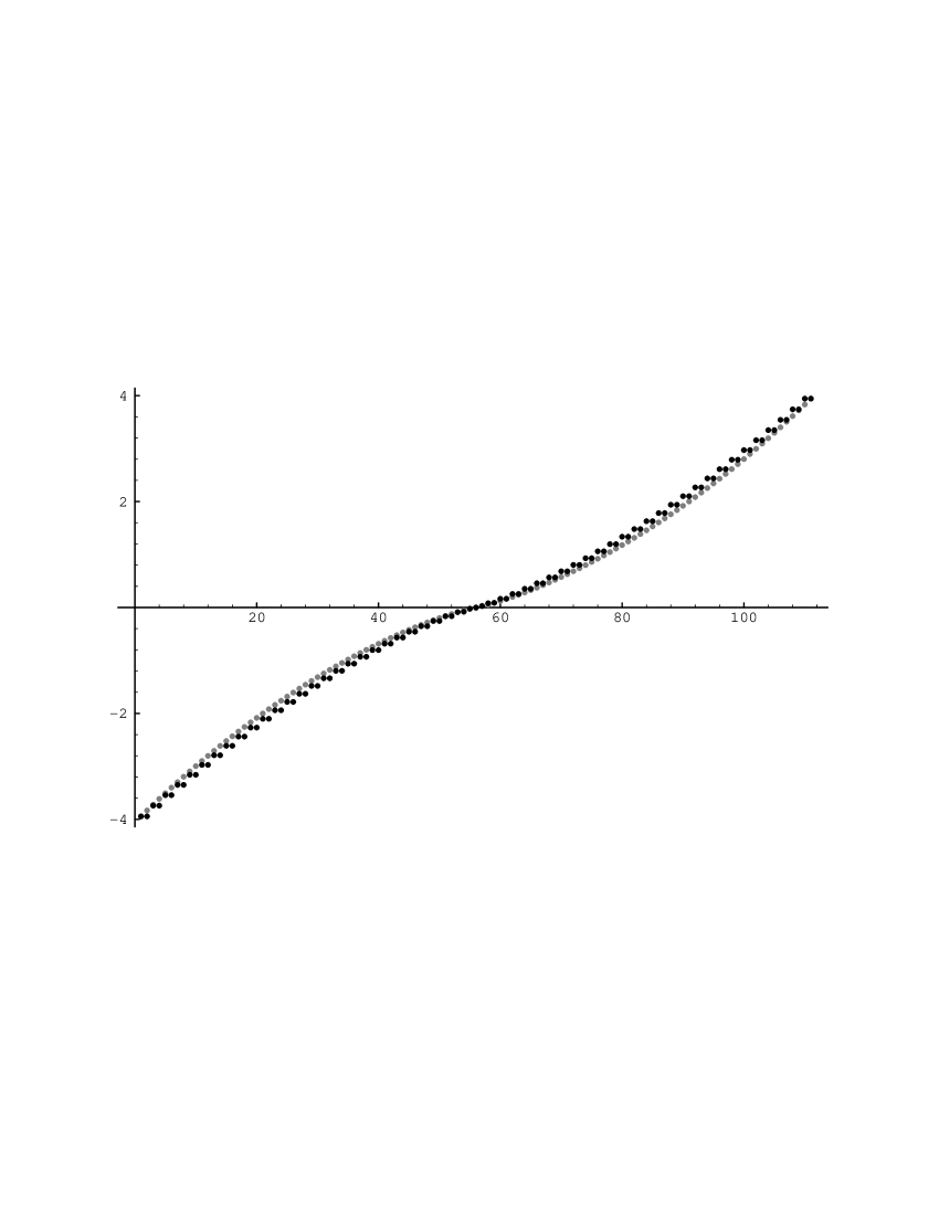
Figure 1: Comparison of the spectra of ${\cal H}_{\mathrm{A}H}$ (grey points) and ${\cal H}_{1}$ (black points), $N=111$.

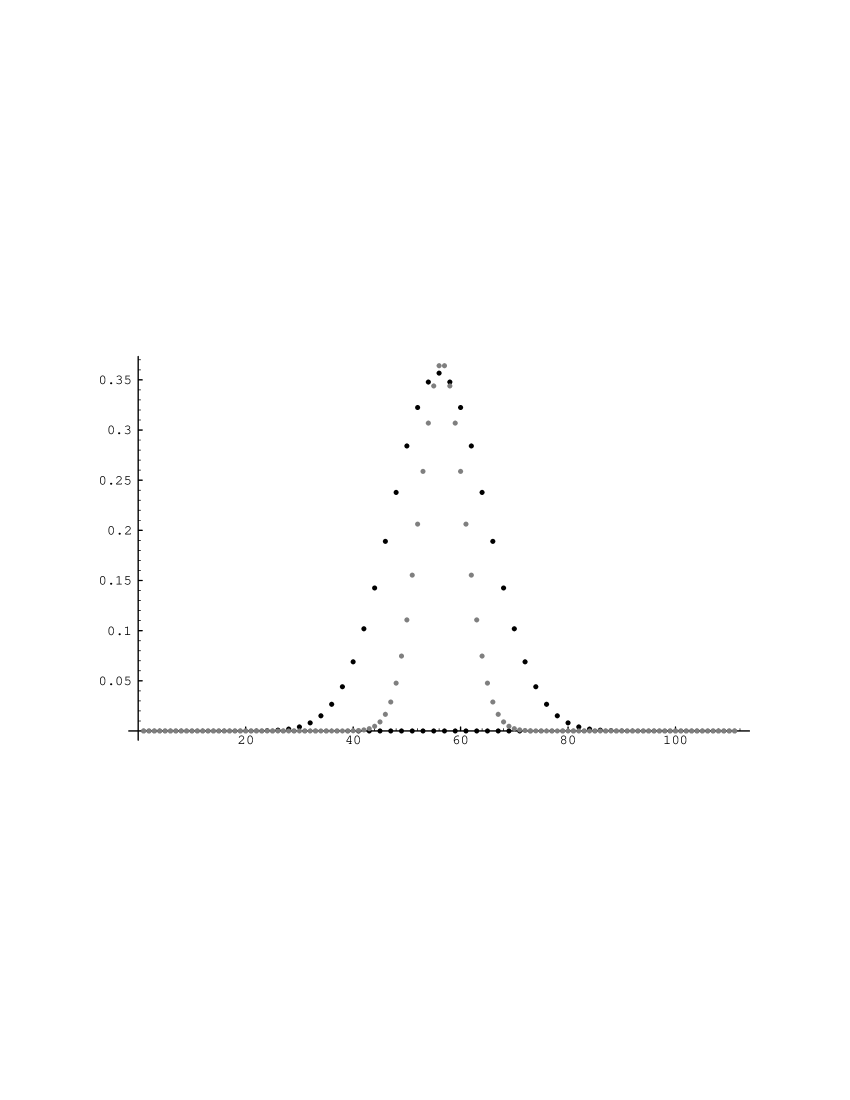
Figure 2: Comparison of the ground state eigenvectors of ${\cal H}_{\mathrm{A}H}$ (grey points) and ${\cal H}_{1}$ (black points), $N=111$.

In fig 3 we give the normalized difference of the two spectra for $N=111$. In fig. 4 we display the maximum error for several values of $N$.

Figure 3: Plot of $E_{{\mathrm{A}H}}(n)-E_{{\cal H}1}(n)\times(E_{{\mathrm{A}H}}(1)/E_{{\cal H}1}(1))$. Note the striking difference between the values of the even and the odd subspaces.

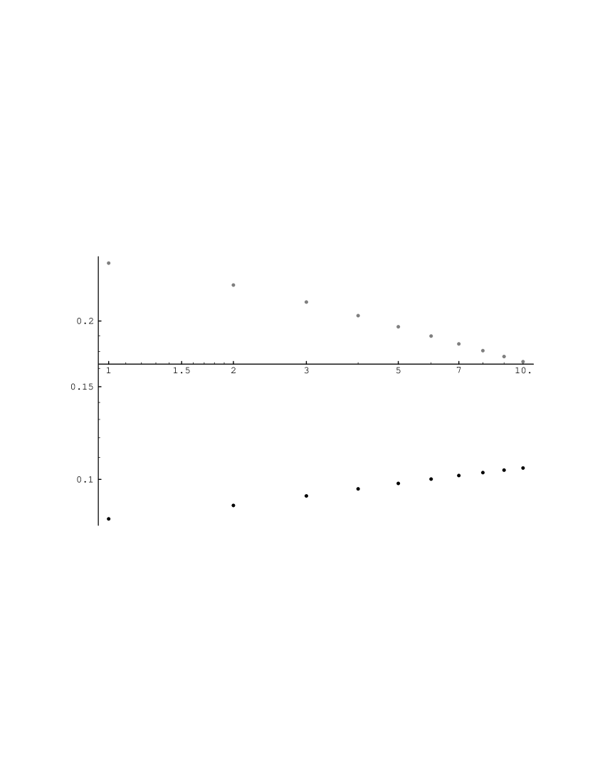
Figure 4: Log-Log plot for the maximum difference for $N=55$ to $N=145$ in steps of 10 for the spectra $E_{{\mathrm{A}H}}$ and $E_{{\cal H}1}$. Black dots are for the even subspaces and gray dots for the odd subspaces of ${\cal H}_{1}$.

7 Conclusions and Perspectives

The main point of this paper is the striking similarity between the spectrum of the AH Hamiltonian and that of our Euler top model. For the moment this is an empirical observation, for which we still lack a physical appreciation from first principles.

From the quantum group symmetry point of view the cyclic character of the $U_{q}(sl(2))$ representations, which appear in this problem would forbid a direct classical large $N$ limit. However, our numerical results indicate that our approximation, through the Euler top, gets better with increasing $N$. This probably suggests some kind of “analytic continuation” between the the Cartesian deformation of $SU(2)$ and the “classical” $SU(2)$ for the root of unity case. This is still an open problem, for which our results seem to indicate a promising direction of attack.

Another problem is the dependence on the Brillouin zone parameters $(k_{x},k_{y})$ as well as on the flux $\phi=2\pi M/N$; indeed we recall that our results hold only for $M=1$ and it is an interesting question, for instance, to calculate the “Hofstadter butterfly” for the Euler top.

We hope to return to these questions in future work.

Acknowledgements: This research was partially supported by the EU grant SCI–0430–C. We would also like to thank the staff of the Laboratoire de Physique Théorique at the Ecole Normale Supérieure for their warm hospitality.

Appendix A Quantum Rotations

In order to construct the three matrices $U_{1}$, $U_{2}$ and $U_{3}$, mentioned in section 3 we have to determine the inner automorphism group of the discrete Heisenberg group matrices ${\cal J}_{r,s}$, i.e. matrices $U(A)$, such that

$$U^{\dagger}(A){\cal J}_{r,s}U(A)=J_{(r,s)A}$$ (71)

where $r,\,s=0,\ldots,N-1$, for every matrix $A\in SL(2,{\bf Z}_{N})$ [22, 23]. It is obvious, from the definition of the generators $J_{1}$, $J_{2}$ and $J_{3}$, that we can construct matrices $U_{1}$, $U_{2}$ and $U_{3}$, if we find three $2\times 2$ matrices $A_{1}$, $A_{2}$ and $A_{3}$, which leave invariant the set of indices$(m,-m)$, $(m,m)$, $(0,1)$ respectively. We check immediately that there exist three abelian subgroups of $SL(2,{\bf Z}_{N})$, which do the job, generated by

$$\begin{array}[]{c}A_{1}=\left(\begin{array}[]{cc}m&m\\ -m&3m\\ \end{array}\right)\\ A_{2}=\left(\begin{array}[]{cc}3m&m\\ -m&m\\ \end{array}\right)\\ A_{3}=\left(\begin{array}[]{cc}1&2\\ 0&1\\ \end{array}\right)\\ \end{array}$$ (72)

We set $U_{i}=U(A_{i})$, with $i=1,2,3$. Using the explicit forms for $U(A),\,A\in SL(2,{\bf Z}_{N})$ from ref. [23], we find

$$\begin{array}[]{ccc}(U_{1})_{k,l}&=&\frac{1}{\sqrt{N}}\omega^{m(l-k)(3l-k-2)}\times\left\{\begin{array}[]{c}1\\ -{\mathrm{i}}\\ \end{array}\right\}\\ (U_{2})_{k,l}&=&\frac{1}{\sqrt{N}}\omega^{m(l-k)(l-3k+2)}\times\left\{\begin{array}[]{c}1\\ -{\mathrm{i}}\\ \end{array}\right\}\\ (U_{3})_{k,l}&=&\delta_{k,l}\omega^{m(k-1)^{2}}\\ \end{array}$$ (73)

where $k,l=1,\ldots,N$ and the symbol

$$\left\{\begin{array}[]{c}1\\ -{\mathrm{i}}\\ \end{array}\right\}\equiv\left\{\begin{array}[]{l}1\,\,N\equiv\,1\,{\mathrm{m}od}\,4\\ -{\mathrm{i}},\,\,N\equiv\,-1\,{\mathrm{m}od}\,4\\ \end{array}\right.$$ (74)

We note finally that the cyclic groups generated by $U_{1}$,$U_{2}$ and $U_{3}$ are of order $N$. The matrices $U_{1}$, $U_{2}$ and $U_{3}$ can be used to define specific discrete Askey-Wilson polynomials as the columns of the matrix

$${\cal P}_{\mathrm{A}W}=U_{1}^{\dagger}U_{2}$$ (75)

cf. the papers of Zhedanov and collaborators in ref. [19].

References

• [1] P. Harper, Proc. Phys. Soc. (London) A265 (1955) 317.
• [2] Ya. Azbel JETP 19 (1964) 634; Phys. Rev. Lett. 43 (1979) 1954.
• [3] J. Zak, Phys. Rev. A134 (1964) 1602.
• [4] W. G. Chambers, Phys. Rev. A 140 (1965) 135.
• [5] D. R. Hofstadter, Phys. Rev. B14 (1976) 2239.
• [6] G. H. Wannier, Phys. Stat. Solid. B88 (1978) 757.
• [7] K. von Klitzing, G. Dorda and M. Pepper, Phys. Rev. Lett. 45 (1980) 494; D. C. Tsui, H. L. Strömer and A. C. Gossard, Phys. Rev. Lett. 48 (1982) 1559.
• [8] R. E. Prange and S. M. Girvin “The Quantum Hall Effect”, Springer-Verlag (1990) second edition.
• [9] N. Aoki, Rep. Prog. Phys. 50 (1987) 655.
• [10] R. B. Laughlin, Phys. Rev. B23 (1981) 5632; Phys. Rev. B27 (1983), 3383.
• [11] S. Aubry and G. Andre, Annals Israel Phys. Soc. 3 (1980) 131.
J. Bellissard and B. Simon, J. Funct. Anal. 48 (1982) 408.
D. J. Thouless, Phys. Rev. B28 (1983) 4272.
F. D. M. Haldane, Phys. Rev. Lett. 51 (1983) 605; Phys. Rev. Lett. 61 (1988) 1029.
M. Wilkinson, Proc. Royal Soc. London A391 (1984) 305.
P. B. Wiegmann, Phys. Rev. Lett. 60 (1988) 821; “Physical Realization of the Parity Anomaly and the Quantum Hall Effect”, preprint NSF-ITP-89-65 (1989).
X. G. Wen and A. Zee, Phys. Rev. Lett. 61 (1988) 1025; Phys. Rev. Lett. 69 (1992) 1811; Phys. Rev. B46 (1992) 2290.
R. Rammal and J. Bellissard, J. Physique (France) 51 (1990) 1803.
D. J. Thouless, Comm. Math. Phys. 127 (1990) 187.
H. Hiramoto and M. Kohmoto, Int. J. Mod.Phys. B6 (1992) 281.
• [12] P. B. Wiegmann and A. Zabrodin, Nucl. Phys. B422 (1994) 495; Phys. Rev. Lett. 72 (1994) 1890; cond-mat/9501129 (1995).
• [13] H. Weyl, The Theory of Groups and Quantum Mechanics, Dover New York (1931).
• [14] D. Fairlie and C. Zachos, Phys. Lett. B224 (1989) 101.
• [15] L. Faddeev and R. M. Kashaev, Comm. Math. Phys. 169 (1995) 181.
• [16] Y. Hatsugai, M. Kohmoto and Y-S. Wu, cond-mat/9405028 (1994).
• [17] M. Jimbo, Lett. Math. Phys. 10 (1985) 63.
• [18] V. V. Bazhanov and Yu. G. Stroganov, J. Stat. Phys. 59 (1990) 333; V. V. Bazhanov, R. M. Kashaev, V. V. Mangazeev and Yu. G. Stroganov, Comm. Math. Phys. 138 (1991) 393.
• [19] E. Witten, Nucl. Phys. B330 (1990) 285;
D. Fairlie, J. Phys. A: Math. Gen. 23 (1990) L183;
Ya. I. Granovskii and A. S. Zhedanov, J. Phys. A: Math. Gen. 26 (1993) L357.
• [20] V. Spiridonov, Lett. Math. Phys. 37 (1996) 173, q-alg/9605033.
• [21] Ph. Roche and D. Arnaudon, Lett. Math. Phys. (1989); D. Arnaudon, hep-th/9203011.
• [22] R. Balian and C. Itzykson, C. R. A. S. (Paris). 303 I(16) (1986) 773.
• [23] G. G. Athanasiu and E. G. Floratos, Nucl. Phys. B425 (1994) 343; Phys. Lett. B352 (1995) 105.
• [24] M. Choi, U. Elliott and N. Yui, Invent. Math. 99 (1990) 225; B. Helfer and J. Sjöstrand Mémoires de la Société Mathématique de France, SMF No. 40, 118 (1990) 1. J. Bellissard, A. van Elst and H. Schulz-Baldes, “The Non-Commutative Geometry of the Quantum Hall Effect”, Lectures given at the University of Crete within the Erasmus Programme “Mathematics and Fundamental Applications” (1994).
• [25] G. G. Athanasiu, E. G. Floratos and S. Nicolis, J. Phys. A: Math. Gen. 29 (1996) 6737, hep-th/9509098.
• [26] O. B. Zaslavskii and V. V. Ul’yanov, Theor. Math. Phys. 71 (1987) 520.
• [27] A. Yu. Morozov, A. M. Perelomov, A. A. Rosly, M. A. Shifman, A. V. Turbiner, Int. J. Mod. Phys. A5 (1990)803; A. V. Turbiner, Comm. Math. Phys. 118 (1988) 467; M. A. Olshanetsky and A. M. Perelomov, Phys. Rep. 71 (1981) 314.
• [28] A. V. Turbiner, J. Phys. A: Math. Gen. 22 (1989) L1; A. V. Turbiner, hep-th/9409068 (1994).
• [29] P. Etingof and A. A. Kirillov Jr. hep-th/9310083 (1993); hep-th/9312101 (1993); hep-th/9312103 (1993).
• [30] E. T. Whittaker and G. N. Watson, Course of Modern Analysis, 4th ed. Cambridge Univ. Press (1958).