CTP-TAMU-27/95

hep-th/9508094

In six spacetime dimensions, the heterotic string is dual to a Type $IIA$ string. On further toroidal compactification to four spacetime dimensions, the heterotic string acquires an $SL(2,Z)_{S}$ strong/weak coupling duality and an $SL(2,Z)_{T}\times SL(2,Z)_{U}$ target space duality acting on the dilaton/axion, complex Kahler form and the complex structure fields $S,T,U$ respectively. Strong/weak duality in $D=6$ interchanges the roles of $S$ and $T$ in $D=4$ yielding a Type $IIA$ string with fields $T,S,U$. This suggests the existence of a third string (whose six-dimensional interpretation is more obscure) that interchanges the roles of $S$ and $U$. It corresponds in fact to a Type $IIB$ string with fields $U,T,S$ leading to a four-dimensional string/string/string triality. Since $SL(2,Z)_{S}$ is perturbative for the Type $IIB$ string, this $D=4$ triality implies $S$-duality for the heterotic string and thus fills a gap left by $D=6$ duality. For all three strings the total symmetry is $SL(2,Z)_{S}\times O(6,22;Z)_{TU}$. The $O(6,22;Z)$ is perturbative for the heterotic string but contains the conjectured non-perturbative $SL(2,Z)_{X}$, where $X$ is the complex scalar of the $D=10$ Type $IIB$ string. Thus four-dimensional triality also provides a (post-compactification) justification for this conjecture. We interpret the $N=4$ Bogomol’nyi spectrum from all three points of view. In particular we generalize the Sen-Schwarz formula for short multiplets to include intermediate multiplets also and discuss the corresponding black hole spectrum both for the $N=4$ theory and for a truncated $S$–$T$–$U$ symmetric $N=2$ theory. Just as the first two strings are described by the four-dimensional elementary and dual solitonic solutions, so the third string is described by the stringy cosmic string solution. In three dimensions all three strings are related by $O(8,24;Z)$ transformations.

July 1995

1 Introduction

An interesting special case of string/string duality [1, 2, 3, 4, 5, 6, 7] is provided by the $D=10$ heterotic string compactified to $D=6$ on $T^{4}$ which is related by strong/weak coupling to the $D=10$ Type $IIA$ string compactified to $D=6$ on $K3$ [8, 9, 10, 11]. The dilaton ${\tilde{\Phi}}$, metric ${\tilde{G}}_{MN}$ and $2$-form ${\tilde{B}}_{MN}$ of the Type $IIA$ theory are related to those of the heterotic theory, $\Phi$, $G_{MN}$ and $B_{MN}$, by [1, 3, 4, 6, 7]

$${\tilde{\Phi}} = -\Phi$$

$${\tilde{G}}_{MN} = e^{-\Phi}G_{MN}$$

$${\tilde{H}} = e^{-\Phi}*H\ ,$$ (1.1)

where $M=0,\ldots,5$, $H=dB+\cdots$, ${\tilde{H}}=d{\tilde{B}}$ and $*$ denotes the Hodge dual. This ensures that the roles of $3$-form field equations and Bianchi identities in one version of the corresponding supergravity theory are interchanged in the other.

After further toroidal compactification to $D=4$ this automatically accounts for the conjectured strong/weak coupling $SL(2,Z)$ duality in the resulting $D=4$, $N=4$ Type $IIA$ string and hence for the $N=4$ Yang-Mills theories obtained by taking the global limit [7]. This is because $S$, the four-dimensional axion/dilaton field, and $T$, the complex Kahler form of the torus, are interchanged in going from the heterotic to the Type $IIA$ theory. Moreover, while the electric field strengths of the Kaluza-Klein gauge fields arising from $G_{MN}$ are the same in both pictures, those of the “winding” gauge fields arising from $B_{MN}$ in the heterotic theory are replaced by their magnetic duals in the Type $IIA$ theory. Thus the strong/weak coupling duality of the Type $IIA$ string is just the target-space $SL(2,Z)_{T}$ of the heterotic string.

However, the target space symmetry of the heterotic theory also contains an $SL(2,Z)_{U}$ that acts on $U$, the complex structure of the torus. This suggests that, in addition to these $S$ and $T$ strings there ought to be a third $U$-string whose axion/dilaton field is $U$ and whose strong/weak coupling duality is $SL(2,Z)_{U}$. From a $D=6$ perspective, this seems strange since, instead of (1.1), we now interchange $G_{45}$ and $B_{45}$. Moreover, of the two electric field strengths which become magnetic, one is a winding gauge field and the other is Kaluza-Klein! So such a duality has no $D=6$ Lorentz invariant meaning. In fact, this $U$ string is a Type $IIB$ string, a result which may also be understood from the point of view of mirror symmetry: interchanging the roles of Kahler form and complex structure (which is equivalent to inverting the radius of one of the two circles) is a symmetry of the heterotic string but takes Type $IIA$ into Type $IIB$ [13, 14]. In summary, if we denote the heterotic, $IIA$ and $IIB$ strings by $H,A,B$ respectively and the axion/dilaton, complex Kahler form and complex structure by the triple $XYZ$ then we have a triality between the $S$-string ($H_{STU}=H_{SUT}$), the $T$-string ($B_{TUS}=A_{TSU}$) and the $U$-string ($A_{UST}=B_{UTS}$) as illustrated in Fig. (1).

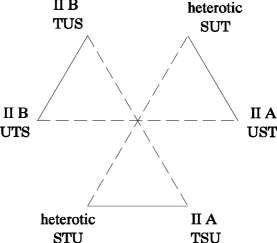
Figure 1: String/string/string triality. The solid lines correspond to string/string dualities and the dashed lines represent mirror transformations.

The field theory limits of the heterotic string on $T^{4}$, the Type $IIA$ string on $K3$ and the Type $IIB$ string on $K3$ are described by certain $N=2,D=6$ supergravity theories described in section (6). As discussed in detail in section (7), each string in $D=4$ will then exhibit the same total symmetry

$$SL(2,Z)_{S}\times O(6,22;Z)_{TU}\supset SL(2,Z)_{S}\times SL(2,Z)_{T}\times SL(2,Z)_{U}\ ,$$ (1.2)

with the $28$ gauge field strengths and their duals transforming as a $(2,28)$, albeit with different interpretations for the three $SL(2,Z)$ factors. Note that there is a discrete symmetry under $T$–$U$ interchange, but there is no such $U$–$S$ or $S$–$T$ symmetry. As discussed in [7], it is the degrees of freedom associated with going from $10$ to $6$ which are responsible for this lack of $S$–$T$–$U$ democracy. This will also be reflected in the Bogomol’nyi spectrum of electric and magnetic states that belong to the short and intermediate $N=4$ supermultiplets. It is therefore instructive to consider first the simpler situation where these modes are truncated out. This we do first in section (2) by truncating the $N=2,D=6$ supergravities to $N=1,D=6$ and then in section (3) by reducing these supergravities to $D=4$. We write down the action which describes the low energy limit of the $S$-string; it exhibits an off-shell (perturbative) $SL(2,Z)_{T}\times SL(2,Z)_{U}$ symmetry and an on-shell (non-perturbative) $SL(2,Z)_{S}$. Similarly, the $T$-string action has an off-shell $SL(2,Z)_{U}\times SL(2,Z)_{S}$ and an on-shell $SL(2,Z)_{T}$, while the $U$-string action has an off-shell $SL(2,Z)_{S}\times SL(2,Z)_{T}$ and an on-shell $SL(2,Z)_{U}$. Aside from the pedagogical usefulness of this $S$–$T$–$U$ symmetric truncation, which describes just $4$ of the $28$ gauge fields, it will turn out that this theory and the resulting $S$–$T$–$U$ symmetric Bogomol’nyi spectrum, discussed in section (5), will find application in $N=2$ theories whose Bogomol’nyi spectrum includes multiplets which were both short and intermediate from the $N=4$ point of view. In particular we discuss the extreme black hole spectrum [15, 16, 17, 18].

In section (5) we provide a soliton interpretation of the three strings. We identify the $S$-string with the elementary string solution of [19], the $T$-string with the dual solitonic string solution of [2] and the $U$-string with (a limit of) the stringy cosmic string solution of [20]. In $D=3$ dimensions, all three strings are related by $O(4,4;Z)$ transformations.

In sections (6), (7), (8) and (9) we repeat the exercise of sections (2), (3), (4) and (5), now including the full set of states. Section (6) describes the three $N=2$, $D=6$ supergravities: the actions in the heterotic and Type $IIA$ cases (together with a duality dictionary relating the two sets of fields) and the equations of motion in the case of Type $IIB$. The compactification to $N=4$, $D=4$ of section (7) reveals one or two surprises: although the $S$-string action has an off-shell $O(6,22;Z)$ which continues to contain $SL(2,Z)_{T}\times SL(2,Z)_{U}$, the $T$-string action has only an off-shell $SL(2,Z)_{U}\times O(3,19;Z)$ which does not contain $SL(2,Z)_{S}$. Similarly, the $U$-string action has only an $SL(2,Z)_{T}\times O(3,19;Z)$ which does not contain $SL(2,Z)_{S}$. In short, none of the actions is $SL(2,Z)_{S}$ invariant! This lack of off-shell $SL(2,Z)_{S}$ in the Type $II$ actions can be traced to the presence of the extra $24$ gauge fields which arise from the R-R sector of Type $II$ strings: $S$-duality in the heterotic picture acts as an on-shell electric/magnetic transformation on all $28$ gauge fields and continues to be an on-shell transformation on the $24$ which remain unchanged under the string/string/string triality.

At first sight, this seems disastrous for deriving the strong/weak coupling duality of the heterotic string from target space duality of the Type $II$ string. The whole point was to explain a non-perturbative symmetry of one string as a perturbative symmetry of another [7]. Fortunately, all is not lost: although $SL(2,Z)_{S}$ is not an off-shell symmetry of the Type $II$ supergravity actions, it is still a symmetry of the Type $II$ string theories. To see this we first note that $D=6$ general covariance is a perturbative symmetry of the Type $IIB$ string and therefore that the $D=4$ Type $IIB$ strings must have a perturbative $SL(2,Z)$ acting on the complex structure of the compactifying torus. Secondly we note that for both Type $IIB$ theories, $B_{TUS}$ and $B_{UTS}$, $S$ is the complex structure field. Thus the $T$ string has $SL(2,Z)_{U}\times SL(2,Z)_{S}$ and the $U$ string has $SL(2,Z)_{S}\times SL(2,Z)_{T}$ as required. In this sense, four-dimensional string/string/string triality fills a gap left by six-dimensional string/string duality: although duality satisfactorily explains the strong/weak coupling duality of the $D=4$ Type $IIA$ string in terms of the target space duality of the heterotic string, the converse requires the Type $IIB$ ingredient.

Note that all of the three $SL(2,Z)_{(S,T,U)}$ take NS-NS states into NS-NS states and that none can be identified with the conjectured non-perturbative $SL(2,Z)_{X}$, where $X$ is the complex scalar of the Type $IIB$ theory in $D=10$, which transforms NS-NS into R-R [22, 8, 9]. However, this $SL(2,Z)_{X}$ is a subgroup of $O(6,22;Z)$. Since this is a perturbative target space symmetry of the heterotic string, the conjecture follows automatically from the $D=4$ string/string/string triality hypothesis. Thus we can say that evidence for this triality is evidence not only for the electric/magnetic duality of all three $D=4$ strings but also for the $SL(2,Z)_{X}$ of the $D=10$ Type $IIB$ string and hence for all the conjectured non-perturbative symmetries of string theory.

In section (8) we describe the $N=4,D=4$ Bogomol’nyi spectrum. We generalize the heterotic string formula of Schwarz and Sen, deriving the two $SL(2,Z)_{S}\times O(6,22;Z)_{TU}$ invariant central charges $Z_{1}$ and $Z_{2}$. This enables us to describe the intermediate multiplets as well as the short ones, and once again we see how the extreme black holes fit into this classification.

Section (9) generalizes (as far as is possible) the soliton interpretation of section (5). But as discussed in [7], including the extra degrees of freedom in going from $10$ to $4$ causes problems in identifying the soliton zero modes. Although it is straightforward to find the heterotic string as a soliton of Type $II$, the converse is more problematical [10, 11]. In three dimensions, the $O(4,4;Z)$ generalizes to $O(8,24;Z)$ [12, 23, 15, 24, 25].

Four-dimensional string/string/string triality was announced by one of us (MJD) at the PASCOS 95 conference in Baltimore and at the SUSY 95 conference in Paris [26]. Related results have been obtained independently by Aspinwall and Morrison [27].

2 $N=1$ supergravity in $D=6$

As a good guide to the kind of dualities one might expect in string theory, it pays to look first at the corresponding supergravity theories. We therefore review some properties of $D=6$ supergravity [28]. The theories of interest, which follow either from $T^{4}$ compactification of the $D=10$ heterotic string or $K3$ compactification of Type $II$, will be $N=2$ supergravities in $D=6$ which yields $N=4$ in $D=4$. All these theories are non-minimal in the sense that they contain additional $N=2$ gauge or matter multiplets. Since such additional matter destroys the $S$–$T$–$U$ symmetry of the four-dimensional string we begin by examining an $N=1$ subset common to all the models of interest. We return to the full $N=2$ theory in section (6).

In terms of six-dimensional $N=1$ representations, we focus on the supergravity multiplet $(G_{MN},\Psi^{+A}{}_{M},B^{+}{}_{MN})$ and the self-dual tensor multiplet $(B^{-}{}_{MN},\chi^{+A},\Phi)$. The index $A=1,2$ labels the $\bf 2$ of $Sp(2)$ and both spinors are symplectic Majorana-Weyl. The $2$-forms $B^{+}{}_{MN}$ and $B^{-}{}_{MN}$ have $3$-form field strengths that are self-dual or anti-self-dual, respectively. Only with the combination of one supergravity multiplet and one self-dual tensor multiplet do we have a conventional Lagrangian formulation. In this case the bosonic fields correspond to the graviton, antisymmetric tensor and dilaton of string theory. This simpler theory will not only serve as a warm-up exercise for understanding the $N=4,D=4$ superstrings but is interesting in its own right for understanding the $N=2,D=4$ strings.

There are three theories to consider, each with the same number of physical degrees of freedom. The first two theories arise from the truncation of the non-chiral $N=2$ supergravity and are related by duality: the first has the usual $3$-form field strength $H$ and the second has the dual field strength ${\tilde{H}}=e^{-\Phi}*H$. The third theory comes from the truncation of the chiral $N=2$ supergravity. While the full chiral $N=2$ theory does not admit a covariant Lagrangian, the $N=1$ truncation, involving the combination of the supergravity and tensor multiplet given above, may be written in a conventional form. In anticipation of their future application, we shall call these theories $H$, $A$ and $B$, respectively.

Denoting the $D=6$ spacetime indices by $(M,N=0,...,5)$, the bosonic part of the usual action takes the form

$$I_{H}=\frac{1}{2\kappa^{2}}\int d^{6}x\sqrt{-G}e^{-\Phi}\left[R_{G}+G^{MN}\partial_{M}\Phi\partial_{N}\Phi-\frac{1}{12}G^{MQ}G^{NR}G^{PS}H_{MNP}H_{QRS}\right]\ .$$ (2.1)

$H$ is the curl of the $2$-form $B$

$$H=dB$$ (2.2)

(at this point there is no Chern-Simons correction). The metric $G_{MN}$ is related to the canonical Einstein metric $G^{c}{}_{MN}$ by

$$G_{MN}=e^{\Phi/2}G^{c}{}_{MN}\ .$$ (2.3)

Similarly, the dual supergravity action is given by

$$I_{A}=\frac{1}{2\kappa^{2}}\int d^{6}x\sqrt{-\tilde{G}}e^{-\tilde{\Phi}}\left[R_{\tilde{G}}+\tilde{G}^{MN}\partial_{M}\tilde{\Phi}\partial_{N}\tilde{\Phi}-\frac{1}{12}\tilde{G}^{MQ}\tilde{G}^{NR}\tilde{G}^{PS}\tilde{H}_{MNP}\tilde{H}_{QRS}\right]\ .$$ (2.4)

$\tilde{H}$ is also the curl of a 2-form $\tilde{B}$

$$\tilde{H}=d\tilde{B}\ .$$ (2.5)

The dual metric $\tilde{G}_{MN}$ is related to the canonical Einstein metric by

$$\tilde{G}_{MN}=e^{\tilde{\Phi}/2}G^{c}{}_{MN}\ .$$ (2.6)

The two supergravities are related by:

$$\tilde{\Phi} = -\Phi$$

$$\tilde{G}_{MN} = e^{-\Phi}G_{MN}$$

$$\tilde{H} = e^{-\Phi}\,{\ast H}\ ,$$ (2.7)

where $\ast$ denotes the Hodge dual. (Since the last equation is conformally invariant, it is not necessary to specify which metric is chosen in forming the dual.) This ensures that the roles of field equations and Bianchi identities in the one version of supergravity are interchanged in the other. The combined field equations and Bianchi identities therefore exhibit a discrete symmetry under interchange of $\Phi\rightarrow-\Phi$, $G\to\tilde{G}$ and $H\rightarrow\tilde{H}$.

Finally, while the third theory is unrelated to the other two (at least in $D=6$), at this level of truncation it has a bosonic action with a form similar to that of $I_{A}$. One subtlety is worth mentioning, however. Since this model arises from a truncation of the compactified Type $IIB$ string which has a complex 3-form field strength in ten dimensions, there is some ambiguity in the identification of the dilaton ${\tilde{\tilde{\Phi}\mkern 0.0mu}\mkern 0.0mu}{}$ and 3-form ${\tilde{\tilde{H}\mkern 4.0mu}\mkern-4.0mu}{}$ of model B, given in the action

$$I_{B}=\frac{1}{2\kappa^{2}}\int d^{6}x\sqrt{-{\tilde{\tilde{G}\mkern 4.0mu}\mkern-4.0mu}{}}e^{-{\tilde{\tilde{\Phi}\mkern 0.0mu}\mkern 0.0mu}{}}\left[R_{{\tilde{\tilde{G}\mkern 4.0mu}\mkern-4.0mu}{}}+{\tilde{\tilde{G}\mkern 4.0mu}\mkern-4.0mu}{}^{MN}\partial_{M}{\tilde{\tilde{\Phi}\mkern 0.0mu}\mkern 0.0mu}{}\partial_{N}{\tilde{\tilde{\Phi}\mkern 0.0mu}\mkern 0.0mu}{}-\frac{1}{12}{\tilde{\tilde{G}\mkern 4.0mu}\mkern-4.0mu}{}^{MQ}{\tilde{\tilde{G}\mkern 4.0mu}\mkern-4.0mu}{}^{NR}{\tilde{\tilde{G}\mkern 4.0mu}\mkern-4.0mu}{}^{PS}{\tilde{\tilde{H}\mkern 4.0mu}\mkern-4.0mu}{}_{MNP}{\tilde{\tilde{H}\mkern 4.0mu}\mkern-4.0mu}{}_{QRS}\right]\ .$$ (2.8)

In particular, the $SL(2,Z)_{X}$ symmetry of the Type $IIB$ supergravity will mix ${\tilde{\tilde{H}\mkern 4.0mu}\mkern-4.0mu}{}$ with its counterpart. Nevertheless, from a stringy viewpoint, we may identify $e^{{\tilde{\tilde{\Phi}\mkern 0.0mu}\mkern 0.0mu}{}}$ as the string loop expansion parameter and ${\tilde{\tilde{H}\mkern 4.0mu}\mkern-4.0mu}{}$ as the 3-form field strength arising from the NS-NS sector of the string. This provides a unique definition of the truncated action, (2.8). Note that there is no $D=6$ Lorentz invariant dictionary between the fields $({\tilde{\tilde{\Phi}\mkern 0.0mu}\mkern 0.0mu}{},{\tilde{\tilde{G}\mkern 4.0mu}\mkern-4.0mu}{},{\tilde{\tilde{H}\mkern 4.0mu}\mkern-4.0mu}{})$ and $(\Phi,G,H)$ or $(\tilde{\Phi},\tilde{G},\tilde{H})$.

3 The $S$-$U$-$T$ symmetric theory in $D=4$

Now let us first consider the H theory, dimensionally reduced to $D=4$. The combination of the six-dimensional $N=1$ supergravity and tensor multiplets reduce to give the $D=4$, $N=2$ graviton multiplet with helicities $(\pm 2,2(\pm{3\over 2}),\pm 1)$ and three vector multiplets with helicities $(\pm 1,2(\pm{1\over 2}),2(0))$. In order to make this explicit, we use a standard decomposition of the six-dimensional metric

$$G_{MN}=\pmatrix{g_{\mu\nu}+A_{\mu}^{m}A_{\nu}^{n}G_{mn}&A_{\mu}^{m}G_{mn}\cr A_{\nu}^{n}G_{mn}&G_{mn}}\ ,$$ (3.1)

where the spacetime indices are ${\mu,\nu}=0,1,2,3$ and the internal indices are $m,n=1,2$. The remaining two vectors arise from the reduced $B$ field

$$B_{MN}=\pmatrix{B_{\mu\nu}+{\textstyle{1\over 2}}(A_{\mu}^{m}B_{m\nu}+B_{\mu n}A_{\nu}^{n})&B_{\mu n}+A_{\mu}^{m}B_{mn}\cr B_{m\nu}+B_{mn}A_{\nu}^{n}&B_{mn}}\ .$$ (3.2)

Four of the six resulting scalars are moduli of the 2-torus. We parametrize the internal metric and $2$-form as

$$G_{mn}=e^{\rho-\sigma}\left(\begin{array}[]{cc}e^{-2\rho}+c^{2}&-c\\ -c&1\end{array}\right)\ ,$$ (3.3)

and

$$B_{mn}=b\,\epsilon_{mn}\ .$$ (3.4)

The four-dimensional metric, given by $g_{\mu\nu}$, is related to the four-dimensional canonical Einstein, $g^{c}_{\mu\nu}$, metric by $g_{\mu\nu}=e^{\eta}g^{c}{}_{\mu\nu}$ where $\eta$ is the four-dimensional shifted dilaton:

$$e^{-\eta}=e^{-\Phi}\sqrt{\det G_{mn}}=e^{-(\Phi+\sigma)}\ .$$ (3.5)

Thus the remaining two scalars are the dilaton $\eta$ and axion $a$ where the axion field $a$ is defined by

$$\epsilon^{\mu\nu\rho\sigma}\partial_{\sigma}a=\sqrt{-g}e^{-\eta}g^{\mu\sigma}g^{\nu\lambda}g^{\rho\tau}H_{\sigma\lambda\tau}\ ,$$ (3.6)

where

$$H_{\sigma\lambda\tau} = 3(\partial_{[\sigma}B_{\lambda\tau]}+\frac{1}{2}A_{[\sigma}^{m}F_{\lambda\tau]m}+\frac{1}{2}B_{m[\sigma}F_{\lambda\tau]}^{m})$$

$$F_{\lambda\tau}^{m} = \partial_{\lambda}A_{\tau}^{m}-\partial_{\tau}A_{\lambda}^{m}$$ (3.7)

$$F_{\lambda\tau m} = \partial_{\lambda}B_{m\tau}-\partial_{\tau}B_{m\lambda}\ .$$

[…] denotes antisymmetrization with weight one.

We may now combine the above six scalars into the complex axion/dilaton field $S$, the complex Kahler form field $T$ and the complex structure field $U$ according to

$$S = S_{1}+iS_{2}=a+ie^{-\eta}$$

$$T = T_{1}+iT_{2}=b+ie^{-\sigma}$$

$$U = U_{1}+iU_{2}=c+ie^{-\rho}\ .$$ (3.8)

This complex parametrization allows for a natural transformation under the various $SL(2,Z)$ symmetries. The action of $SL(2,Z)_{S}$ is given by

$$S\rightarrow\frac{aS+b}{cS+d}\ ,$$ (3.9)

where $a,b,c,d$ are integers satisfying $ad-bc=1$, with similar expressions for $SL(2,Z)_{T}$ and $SL(2,Z)_{U}$. Defining the matrices ${\cal M}_{S}$, ${\cal M}_{T}$ and ${\cal M}_{U}$ via

$${\cal M}_{S}=\frac{1}{S_{2}}\left(\begin{array}[]{cc}1&S_{1}\\ S_{1}&|S|^{2}\end{array}\right)\ ,$$ (3.10)

the action of $SL(2,Z)_{S}$ now takes the form

$${\cal M}_{S}\rightarrow\omega_{S}{}^{T}{\cal M}_{S}\omega_{S}\ ,$$ (3.11)

where

$$\omega_{S}=\left(\begin{array}[]{cc}d&b\\ c&a\end{array}\right)\ ,$$ (3.12)

with similar expressions for ${\cal M}_{T}$ and ${\cal M}_{U}$. We also define the $SL(2,Z)$ invariant tensors

$$\epsilon_{S}=\epsilon_{T}=\epsilon_{U}=\left(\begin{array}[]{cc}0&1\\ -1&0\end{array}\right)\ .$$ (3.13)

The fundamental supergravity (2.1) now becomes

$$I_{STU} = \frac{1}{16\pi G}\int d^{4}x\sqrt{-g}e^{-\eta}\Bigl{[}R_{g}+g^{\mu\nu}\partial_{\mu}\eta\partial_{\nu}\eta-\frac{1}{12}g^{\mu\lambda}g^{\nu\tau}g^{\rho\sigma}H_{\mu\nu\rho}H_{\lambda\tau\sigma}$$ (3.14)

$$\kern 93.00017pt+\frac{1}{4}{\rm Tr}(\partial{\cal M}_{T}{}^{-1}\partial{\cal M}_{T})+\frac{1}{4}{\rm Tr}(\partial{\cal M}_{U}{}^{-1}\partial{\cal M}_{U})$$

$$\kern 93.00017pt-\frac{1}{4}{F_{S}}_{\mu\nu}{}^{T}({\cal M}_{T}\times{\cal M}_{U}){F_{S}}^{\mu\nu}\Bigr{]}\ .$$

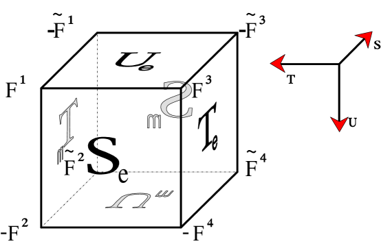
Figure 2: The cube of triality. All field strengths are given in $S$-variables.

The four $U(1)$ gauge fields $A_{S}^{a}$ are given by ${A_{S}^{1}}_{\mu}=B_{4\mu},\,{A_{S}^{2}}_{\mu}=B_{5\mu},\,{A_{S}^{3}}_{\mu}=A_{\mu}^{5},\,{A_{S}^{4}}_{\mu}=-A_{\mu}^{4}$. The three-form becomes $H_{\mu\nu\rho}=3(\partial_{[\mu}B_{\nu\rho]}-{\textstyle{1\over 2}}A_{S[\mu}{}^{T}(\epsilon_{T}\times\epsilon_{U}){F_{S}}_{\nu\rho]})$. This action is manifestly invariant under $T$-duality and $U$-duality, with

$${F_{S}}_{\mu\nu}\rightarrow(\omega_{T}{}^{-1}\times\omega_{U}{}^{-1}){F_{S}}_{\mu\nu}\ ,\,\qquad{\cal M}_{T/U}\rightarrow\omega_{T/U}^{T}\,{\cal M}_{T/U}\,\omega_{T/U}\ ,$$ (3.15)

and with $\eta$, $g_{\mu\nu}$ and $B_{\mu\nu}$ inert. Its equations of motion and Bianchi identities (but not the action itself) are also invariant under $S$-duality, with $T$ and $g^{c}{}_{\mu\nu}$ inert and with

$$\left(\begin{array}[]{c}{{F_{S}}}_{\mu\nu}{}^{a}\\ {\widetilde{F}_{S}}{}_{\mu\nu}{}^{a}\end{array}\right)\rightarrow\omega_{S}^{-1}\left(\begin{array}[]{c}{{F_{S}}}_{\mu\nu}{}^{a}\\ {\widetilde{F}_{S}}{}_{\mu\nu}{}^{a}\end{array}\right)\ ,$$ (3.16)

where

$${\widetilde{F}_{S}}{}_{\mu\nu}{}^{a}=-S_{2}[({\cal M}_{T}{}^{-1}\times{\cal M}_{U}{}^{-1})(\epsilon_{T}\times\epsilon_{U})]^{a}{}_{b}*{F_{S}}_{\mu\nu}{}^{b}-S_{1}{F_{S}}_{\mu\nu}{}^{a}\ .$$ (3.17)

Thus $T$-duality transforms Kaluza-Klein electric charges $({F_{S}}^{3},{F_{S}}^{4})$ into winding electric charges $({F_{S}}^{1},{F_{S}}^{2})$ (and Kaluza-Klein magnetic charges into winding magnetic charges), $U$-duality transforms the Kaluza-Klein and winding electric charge of one circle $({F_{S}}^{3},{F_{S}}^{2})$ into those of the other $({F_{S}}^{4},{F_{S}}^{1})$ (and similarly for the magnetic charges) but $S$-duality transforms Kaluza-Klein electric charge $({F_{S}}^{3},{F_{S}}^{4})$ into winding magnetic charge $({\tilde{F_{S}}}^{3},{\tilde{F_{S}}}^{4})$ (and winding electric charge into Kaluza-Klein magnetic charge). In summary we have $SL(2,Z)_{T}\times SL(2,Z)_{U}$ and $T\leftrightarrow U$ off-shell but $SL(2,Z)_{S}\times SL(2,Z)_{T}\times SL(2,Z)_{U}$ and an $S$–$T$–$U$ interchange on-shell. The $S\leftrightarrow T$ part arises from the discrete on-shell symmetry $\Phi\rightarrow-\Phi$, $G\to\tilde{G}$ and $H\rightarrow\tilde{H}$ in $D=6$.

Now consider the two actions obtained by cyclic permutation of the fields $S,T,U$:

$$I_{TUS} = \frac{1}{16\pi G}\int d^{4}x\sqrt{-{\tilde{g}}}e^{-\sigma}\Bigl{[}R_{\tilde{g}}+{\tilde{g}}^{\mu\nu}\partial_{\mu}\sigma\partial_{\nu}\sigma-\frac{1}{12}{\tilde{g}}^{\mu\lambda}{\tilde{g}}^{\nu\tau}{\tilde{g}}^{\rho\sigma}{\tilde{H}}_{\mu\nu\rho}{\tilde{H}}_{\lambda\tau\sigma}$$ (3.18)

$$\kern 93.00017pt+\frac{1}{4}{\rm Tr}(\partial{\cal M}_{U}{}^{-1}\partial{\cal M}_{U})+\frac{1}{4}{\rm Tr}(\partial{\cal M}_{S}{}^{-1}\partial{\cal M}_{S})$$

$$\kern 93.00017pt-\frac{1}{4}{F_{T}}_{\mu\nu}{}^{T}({\cal M}_{U}\times{\cal M}_{S}){F_{T}}^{\mu\nu}\Bigr{]}\ ,$$

and

$$I_{UST} = \frac{1}{16\pi G}\int d^{4}x\sqrt{-{\tilde{\tilde{g}\mkern 3.0mu}\mkern-3.0mu}{}}e^{-\rho}\Bigl{[}R_{{\tilde{\tilde{g}\mkern 3.0mu}\mkern-3.0mu}{}}+{\tilde{\tilde{g}\mkern 3.0mu}\mkern-3.0mu}{}^{\mu\nu}\partial_{\mu}\rho\partial_{\nu}\rho-\frac{1}{12}{\tilde{\tilde{g}\mkern 3.0mu}\mkern-3.0mu}{}^{\mu\lambda}{\tilde{\tilde{g}\mkern 3.0mu}\mkern-3.0mu}{}^{\nu\tau}{\tilde{\tilde{g}\mkern 3.0mu}\mkern-3.0mu}{}^{\rho\sigma}{\tilde{\tilde{H}\mkern 4.0mu}\mkern-4.0mu}{}_{\mu\nu\rho}{\tilde{\tilde{H}\mkern 4.0mu}\mkern-4.0mu}{}_{\lambda\tau\sigma}$$ (3.19)

$$\kern 93.00017pt+\frac{1}{4}{\rm Tr}(\partial{\cal M}_{S}{}^{-1}\partial{\cal M}_{S})+\frac{1}{4}{\rm Tr}(\partial{\cal M}_{T}{}^{-1}\partial{\cal M}_{T})$$

$$\kern 93.00017pt-\frac{1}{4}{F_{U}}_{\mu\nu}{}^{T}({\cal M}_{S}\times{\cal M}_{T}){F_{U}}^{\mu\nu}\Bigr{]}\ .$$

The $D=6$ interpretation of these actions is as follows. The action $I_{TSU}=I_{TUS}$ is obtained by reducing the dual $A$ theory (2.4), where the four dimensional dual metric is given by ${\tilde{g}}_{\mu\nu}=e^{\sigma}g^{c}{}_{\mu\nu}$ and the $3$-form field strength ${\tilde{H}}$ is related to the pseudoscalar field $b$ by

$$\epsilon^{\mu\nu\rho\sigma}\partial_{\sigma}b=\sqrt{-\tilde{g}}e^{-\sigma}\tilde{g}^{\mu\sigma}\tilde{g}^{\nu\lambda}\tilde{g}^{\rho\tau}\tilde{H}_{\sigma\lambda\tau}\ .$$ (3.20)

However, since mirror symmetry interchanges $A$ and $B$ it also yields the field equations obtained by reducing the field equations of the $B$ theory but with $S$ and $U$ interchanged. Similarly, the action $I_{UST}=I_{UTS}$ yields the field equations obtained by reducing the $B$ theory, where the four dimensional metric is now given by ${\tilde{\tilde{g}\mkern 3.0mu}\mkern-3.0mu}{}_{\mu\nu}=e^{\rho}g^{c}{}_{\mu\nu}$ and the $3$-form field strength ${\tilde{\tilde{H}\mkern 4.0mu}\mkern-4.0mu}{}$ is related to the pseudoscalar field $c$ by

$$\epsilon^{\mu\nu\rho\sigma}\partial_{\sigma}c=\sqrt{-{\tilde{\tilde{g}\mkern 3.0mu}\mkern-3.0mu}{}}e^{-\rho}{{\tilde{\tilde{g}\mkern 3.0mu}\mkern-3.0mu}{}}^{\mu\sigma}{{\tilde{\tilde{g}\mkern 3.0mu}\mkern-3.0mu}{}}^{\nu\lambda}{{\tilde{\tilde{g}\mkern 3.0mu}\mkern-3.0mu}{}}^{\rho\tau}{{\tilde{\tilde{H}\mkern 4.0mu}\mkern-4.0mu}{}}_{\sigma\lambda\tau}\ .$$ (3.21)

Once again, however, by mirror symmetry this is equivalent to reducing the $A$ theory with $S$ and $T$ interchanged. The relation between the field strengths ${F_{S}}$, ${F_{T}}$ and ${F_{U}}$ is given in Table 1 and Figure 2. Figure 2 visualizes the connection of all three strings. Each side of the cube corresponds to electric or magnetic $S$, $T$ or $U$ strings. Each dimension is related to one duality. To get from one side to an adjacent one, two fields need to be dualized. Mirror symmetry takes the cube into its mirror.

$$\begin{array}[]{ccccccc}\rm axion/&\rm Kahler&\rm complex&\hfil\rm gauge\ fields\hfil\\ \rm dilaton&\rm form&\rm structure&&&&\\ &&&&&&\\ S&T&U&{F_{S}}^{3}&-{F_{S}}^{4}&{F_{S}}^{1}&-{F_{S}}^{2}\\ S&U&T&{F_{S}}^{3}&F_{S}^{1}&-{F_{S}}^{4}&-{F_{S}}^{2}\\ U&S&T&{F_{S}}^{3}&{F_{S}}^{1}&-{\tilde{F_{S}}}^{3}&-\tilde{F_{S}}^{1}\\ U&T&S&{F_{S}}^{3}&-\tilde{F_{S}}^{3}&{F_{S}}^{1}&-\tilde{F_{S}}^{1}\\ T&U&S&{F_{S}}^{3}&-\tilde{F}_{S}^{3}&-F_{S}^{4}&\tilde{F}_{S}^{4}\\ T&S&U&{F_{S}}^{3}&-F_{S}^{4}&-\tilde{F}_{S}^{3}&{\tilde{F}_{S}}^{4}\end{array}$$

Table 1: Triality

4 The Bogomol’nyi Spectrum

It is now straightforward to write down an $S$–$U$–$T$ symmetric Bogomol’nyi mass formula. Let us define electric and magnetic charge vectors $\alpha_{S}^{a}$ and $\beta_{S}^{a}$ associated with the field strengths ${{F_{S}}}^{a}$ and ${\tilde{F_{S}}}^{a}$ in the standard way. The electric and magnetic charges $Q_{S}^{a}$ and $P_{S}^{a}$ are given by

$${F_{S}}_{0r}^{a}\sim\frac{Q_{S}^{a}}{r^{2}}\,\qquad*{F_{S}}_{0r}^{a}\sim\frac{P_{S}^{a}}{r^{2}}\ ,$$ (4.1)

giving rise to the charge vectors

$$\pmatrix{\alpha_{S}^{a}\cr\beta_{S}^{a}}=\pmatrix{S_{2}^{(0)}{\cal M}_{T}^{-1}\times{\cal M}_{U}^{-1}&S_{1}^{(0)}\epsilon_{T}\times\epsilon_{U}\cr 0&-\epsilon_{T}\times\epsilon_{U}}^{ab}\pmatrix{Q_{S}^{b}\cr P_{S}^{b}}.$$ (4.2)

For our purpose it is useful to define a generalized charge vector $\gamma^{a{\tilde{a}}{\tilde{\tilde{a}}}}$ via

$$\left(\begin{array}[]{c}\gamma^{111}\\ \gamma^{112}\\ \gamma^{121}\\ \gamma^{122}\\ \gamma^{211}\\ \gamma^{212}\\ \gamma^{221}\\ \gamma^{222}\end{array}\right)=\left(\begin{array}[]{c}-\beta_{S}^{1}\\ -\beta_{S}^{2}\\ -\beta_{S}^{3}\\ -\beta_{S}^{4}\\ \alpha_{S}^{1}\\ \alpha_{S}^{2}\\ \alpha_{S}^{3}\\ \alpha_{S}^{4}\end{array}\right)\ ,$$ (4.3)

transforming as

$$\gamma^{a{\tilde{a}}{\tilde{\tilde{a}}}}\rightarrow\omega_{S}{}^{a}{}_{b}\omega_{T}{}^{\tilde{a}}{}_{\tilde{b}}\omega_{U}{}^{\tilde{\tilde{a}}}{}_{\tilde{\tilde{b}}}\gamma^{b{\tilde{b}}{\tilde{\tilde{b}}}}\ .$$ (4.4)

Then the mass formula is

$$m^{2}=\frac{1}{16}\gamma^{T}({\cal M}_{S}{}^{-1}{\cal M}_{T}{}^{-1}{\cal M}_{U}{}^{-1}-{\cal M}_{S}{}^{-1}{\epsilon}_{T}{\epsilon}_{U}-{\epsilon}_{S}{\cal M}_{T}{}^{-1}{\epsilon}_{U}-{\epsilon}_{S}{\epsilon}_{T}{\cal M}_{U}{}^{-1})\gamma\ .$$ (4.5)

Although all three theories have the same mass spectrum, there is clearly a difference of interpretation with electrically charged elementary states in one picture being solitonic monopole or dyon states in the other. This agrees with the $N=2$ Bogomol’nyi formula of Ceresole et al. [29] and is a truncation of the generalized $N=4$ mass formula derived from first principles in section (8). Note, however, that this is not a truncation of the $N=4$ Bogomol’nyi formula of Schwarz and Sen [30, 31]. In particular, we note that although both formulas have $SL(2,Z)_{S}\times SL(2,Z)_{T}\times SL(2,Z)_{U}$, even the truncated Schwarz-Sen formula (8.15) is only symmetric under $T$–$U$ interchange and not $S$–$T$–$U$. To understand this, we recall that in $N=4$ supersymmetry, we have two central charges $Z_{1}$ and $Z_{2}$. There are three kinds of massive multiplets: short, intermediate and long according as $(m=|Z_{1}|=|Z_{2}|)$, $(m=|Z_{1}|>|Z_{2}|)$ or $(m>|Z_{1}|,|Z_{2}|)$. The Schwarz-Sen formula refers only to the short multiplets. In $N=2$, however, we have only one central charge $Z$. There are only short and long multiplets according as $m=|Z|$ or $m>|Z|$. States that were only intermediate in the $N=4$ theory may thus become short in the truncation to $N=2$.

A nice example of this phenomenon is provided by the extreme Reissner-Nordstrom black hole (dilaton coupling $a=0$) which in string theory is dyonic with charge vectors $\alpha=(1,0,0,-1)$ and $\beta=(0,-1,-1,0)$ [15]. It belongs to an intermediate multiplet in the $N=4$ theory and is therefore absent from the Sen-Schwarz spectrum but belongs to a short multiplet in the $N=2$ theory and appears in the spectrum (4.5). The two $N=4$ central charges are given in section (8). Since we have identified the Reissner-Nordstrom black hole in the $N=2$ spectrum, it is natural to ask which other black holes satisfy (4.5). Besides $a=0$, the supersymmetric dilaton coupling parameters are $a=\sqrt{3},1,1/\sqrt{3}$ [32, 15, 33, 34]. It turns out that all of the corresponding states indeed satisfy the Bogomol’nyi bound and therefore preserve 1/2 of the supersymmetries in the $N=2$ theory. The $a=\sqrt{3}$ black hole has charge vectors $\alpha=(1,0,0,0)$, $\beta=(0,0,0,0)$. To cut a long story short we set all the VEV’s to zero and find its mass to be (in our units) $m=1/4$, according to

$$m^{2}=\frac{Q^{2}}{4(1+a^{2})}\ ,$$ (4.6)

where $Q$ is the charge of the effective field strength. Mass and charges are obviously related by (4.5). The mass of the electrically charged $a=1$ black hole with $\alpha=(1,0,0,-1)$ is $m=1/2$ [15] which agrees also with (4.5). Like the $a=\sqrt{3}$ black hole, this solution is elementary for the S-string, but it is dyonic for the $T$- and $U$-strings. Further dynamical evidence for the identification of $a=\sqrt{3}$ and $a=1$ black holes with elementary heterotic $N_{L}=1$ and $N_{L}>1$ string states [15] has recently been given in [34]. Finally, the $a=1/\sqrt{3}$ black hole is dyonic in all pictures. Its charge vectors are $\alpha=(1,0,0,-1)$ and $\beta=(0,-1,0,0)$. The mass is $m=3/4$ which can be verified by truncating the supergravity theory to one effective field strength $\sqrt{3}F=F_{S}^{1}=-F_{S}^{4}=\tilde{F}_{S}^{2}$ along the lines of [15]. A quick comparison with the Bogomol’nyi formula proves that the $a=1/\sqrt{3}$ black hole preserves indeed 1/2 of the supersymmetries in $N=2$. As described in [15], the mass and charge assignments of the $a=\sqrt{3},1,1/\sqrt{3}$ and $0$ black holes are compatible with their interpretations as $1,2,3$ and $4$-particle bound states with zero binding energy.

5 Soliton Interpretation

Four-dimensional string/string/string/triality suggests that it ought to be possible to describe the $S$-string, $T$-string and $U$-string as elementary and solitonic solutions directly in four dimensions. This is indeed the case. The $H$ action (2.1) admits as an elementary solution the $S$-string

$$ds^{2} = e^{\eta}(-d\tau^{2}+d\sigma^{2})+dzd\bar{z}$$

$$S = a+ie^{-\eta}=\frac{1}{2\pi i}\ln\frac{r}{r_{0}}\ ,$$ (5.1)

where $z=x_{2}+ix_{3}$ corresponds to the transverse directions and $r=|z|$. It also admits as a soliton solution the dual $T$-string

$$ds^{2} = -d\tau^{2}+d\sigma^{2}+e^{-\sigma}dzd\bar{z}$$

$$T = b+ie^{-\sigma}=\frac{1}{2\pi i}\ln\frac{r}{r_{0}}\ .$$ (5.2)

Furthermore, it admits as a soliton solution the $U$-string

$$ds^{2} = -d\tau^{2}+d\sigma^{2}+e^{-\rho}dzd\bar{z}$$

$$U = c+ie^{-\rho}=\frac{1}{2\pi i}\ln\frac{r}{r_{0}}\ .$$ (5.3)

We recognize the $S$-string as the elementary string solution of [19] and the $T$-string as the dual string solution of [2] but the $U$-string is given by a limit of the stringy cosmic string of [20] where the fields $\rho$ and $c$ are simply given by the internal metric

$$\sqrt{G}G^{-1}={\cal M}_{U}=e^{\rho}\left(\begin{array}[]{cc}1&c\\ c&c^{2}+e^{-2\rho}\end{array}\right)\ .$$ (5.4)

Consequently, the $U$-string is a solution of pure gravity in $D=6$ as discussed in [20].

It follows that the $A$ action (2.4) admits the $T$-string as the elementary solution and the $S$- and $U$-strings as the solitonic solutions and that the $B$ action (2.8) admits the $U$-string as the elementary solution and the $T$- and $S$-strings as the solitonic solutions. Note that we may generate new $S$, $T$- and $U$-string solutions by making $SL(2,Z)_{S}$ transformations on (5.1), $SL(2,Z)_{T}$ transformations on (5.2) and $SL(2,Z)_{U}$ transformations on (5.3). So there is really an $SL(2,Z)$ family of solutions for each string. Once again, all this is consistent with string/string/string triality.

The fundamental string solution given in (5.1) corresponds to the case where all four gauge fields $(F_{S}{}^{1},F_{S}{}^{2},F_{S}{}^{3},F_{S}{}^{4})$ have been set to zero. But as described in [35] a more general solution with non-vanishing gauge fields may be generated by making $O(3,3)$ transformations on the neutral solution. Such deformations are possible since the original solution is independent of $x^{0}$ as well as $x^{4}$ and $x^{5}$. However, since we want to keep the asymptotic values of the field configurations fixed, this leaves us with an $O(2,1)\times O(2,1)$ subgroup. Not every element of this subgroup generates a new solution; there is an $O(2)\times O(2)$ subgroup that leaves the solution invariant. Thus the number of independent deformations is given by the dimension of the coset space $O(2,1)\times O(2,1)/O(2)\times O(2)$ which is equal to four, corresponding to the four electric charges of $U(1)^{4}$. Exactly analogous statements now apply to the $T$-string (5.3) and $U$-string (5.3) solutions.

All of the above transformations take each string into itself. We now consider transformations that map one string into another. If we compactify the $H$ action (2.1) to three dimensions on $T^{3}$ the on-shell $SL(2,Z)_{S}$ will combine with the off-shell $O(3,3;Z)$ target space duality to form an on-shell $O(4,4;Z)$. Similar remarks apply to the $A$ and $B$ actions. It follows that all three strings are mapped into one another by $O(4,4;Z)$ transformations. That the stringy cosmic string was related to the elementary string in this way was pointed out in [24]; that the dual string was also related in this way was pointed out in [25].

6 $N=2$ supergravity in $D=6$

The preceding discussion has shown an interesting triality structure of the $H$, $A$ and $B$ theories when compactified to four dimensions. However, until now we have omitted the additional $D=6$ matter and/or gauge fields present in all models. In this section we examine the full $D=6$, $N=2$ theories, and in the next section we incorporate the additional fields into string/string/string triality.

We begin by focusing on the heterotic string compactified on a generic torus to $D=6$ [36, 37]. The low-energy limit of this theory is described by a non-chiral $N=2$ supergravity with one graviton multiplet and 20 Yang-Mills multiplets. The bosonic action is given by

$$I_{H} = \frac{1}{2\kappa^{2}}\int d^{6}x\sqrt{-G}e^{-\Phi}\Bigl{[}R_{G}+G^{MN}\partial_{M}\Phi\partial_{N}\Phi-\frac{1}{12}G^{MQ}G^{NR}G^{PS}H_{MNP}H_{QRS}$$ (6.1)

$$\kern 40.00006pt+\frac{1}{8}G^{MN}{\rm Tr}(\partial_{M}ML\partial_{N}ML)-\frac{1}{4}G^{MP}G^{NQ}F_{MN}{}^{a}(LML)_{ab}F_{PQ}{}^{b}\Bigr{]}\ ,$$

where $A_{M}{}^{a}$ are $24$ abelian gauge fields and $H_{MNP}=3(\partial_{[M}B_{NP]}+{\textstyle{1\over 2}}A_{[M}{}^{a}L_{ab}F_{NP]}{}^{b})$. The 80 scalars parametrize an $O(4,20)/O(4)\times O(20)$ coset and are combined into the symmetric $24\times 24$ dimensional matrix $M$ satisfying $MLM=L$ where $L$ is the invariant metric on $O(4,20)$:

$$L=\pmatrix{0&I_{4}&0\cr I_{4}&0&0\cr 0&0&-I_{16}}\ .$$ (6.2)

The action is invariant under the $O(4,20;Z)$ target space duality transformations $M\rightarrow\Omega M\Omega^{T}$, $A_{\mu}{}^{a}\rightarrow\Omega^{a}{}_{b}A_{\mu}{}^{b}$, $G_{\mu\nu}\rightarrow G_{\mu\nu}$, $B_{\mu\nu}\rightarrow B_{\mu\nu}$, $\Phi\rightarrow\Phi$, where $\Omega$ is an $O(4,20;Z)$ matrix satisfying $\Omega^{T}L\Omega=L$. The full $I_{H}$ action is invariant under non-chiral six-dimensional $N=2$ supersymmetry transformations. For convenience in writing down fermionic equations, we use an underlying $D=10$ notation where the four $D=6$ symplectic Majorana-Weyl spinors of the $N=2$ theory may be combined into a ten-dimensional Majorana-Weyl spinor $\epsilon$. Since we will need the supersymmetry transformations of the gravitino and dilatino when deriving the Bogomol’nyi mass bound, we list them here:

$$\delta\psi_{M} = \left[\nabla_{M}-{1\over 8}H_{MNP}\Gamma^{NP}+{1\over 2\sqrt{2}}(VLF)_{R\,MN}^{\overline{a}}\Gamma^{N}\Gamma^{\overline{a}}-{1\over 4}(\partial_{M}^{\vphantom{-1}}V_{R}^{\vphantom{-1}}V^{-1}_{R})^{\overline{a}}{}_{\overline{b}}\Gamma^{\overline{a}\overline{b}}\right]\epsilon$$

$$\delta\lambda = -{1\over 4\sqrt{2}}\left[\Gamma^{M}\partial_{M}\Phi-{1\over 6}H_{MNP}\Gamma^{MNP}+{1\over 2\sqrt{2}}(VLF)_{R\,MN}^{\overline{a}}\Gamma^{MN}\Gamma^{\overline{a}}\right]\epsilon\ ,$$ (6.3)

where the Dirac matrices may be given a ten-dimensional interpretation, $\Gamma^{(10)}=\{\Gamma^{A},\Gamma^{\overline{a}}\}$, with six-dimensional Dirac matrices $\Gamma_{M}=E_{M}^{A}\Gamma^{A}$ [38].

Turning to the Type $IIA$ string compactified on $K3$, we find an identical massless spectrum, corresponding to one $N=2$ supergravity multiplet coupled to 20 $N=2$ Yang-Mills multiplets [39]. This time the action is given by

$$I_{A} = \frac{1}{2\kappa^{2}}\int d^{6}x\sqrt{-\tilde{G}}e^{-{\tilde{\Phi}}}\Bigl{[}R_{\tilde{G}}+\tilde{G}^{MN}\partial_{M}{\tilde{\Phi}}\partial_{N}{\tilde{\Phi}}-\frac{1}{12}\tilde{G}^{MQ}\tilde{G}^{NR}\tilde{G}^{PS}\tilde{H}_{MNP}\tilde{H}_{QRS}$$ (6.4)

$$\kern 60.00009pt+\frac{1}{8}{\tilde{G}}^{MN}{\rm Tr}(\partial_{M}{\tilde{M}}L\partial_{N}{\tilde{M}}L)-{1\over 4}e^{\tilde{\Phi}}\tilde{G}^{MP}\tilde{G}^{NQ}\tilde{F}_{MN}^{a}(L\tilde{M}L)_{ab}\tilde{F}_{PQ}{}^{b}\Bigr{]}$$

$$-{1\over 2\kappa^{2}}\int d^{6}x{1\over 16}\epsilon^{MNPQRS}\tilde{B}_{MN}\tilde{F}_{PQ}{}^{a}L_{ab}\tilde{F}_{RS}{}^{b}\ ,$$

where now ${\tilde{H}}$ has no Chern-Simons corrections, ${\tilde{H}}=d{\tilde{B}}$. The action (6.4) has the same $O(4,20;Z)$ symmetry as (6.1) [40]. In particular, the matrix $\tilde{M}$ of scalars satisfies the constraint $\tilde{M}L\tilde{M}=L$.

Under heterotic/Type $IIA$ duality we have the following dictionary [7, 9] relating the two sets of fields:

$${\tilde{\Phi}} = -\Phi$$

$${\tilde{G}}_{MN} = e^{-\Phi}G_{MN}$$

$${\tilde{H}} = e^{-\Phi}*H$$ (6.5)

$$\tilde{A}_{M} = A_{M}$$

$$\tilde{M} = M\ .$$ (6.6)

This gives, in particular, the Type $IIA$ gravitino and dilatino supersymmetry transformations

$$\delta\tilde{\psi}_{M} = \Biggl{[}\tilde{\nabla}_{M}-{1\over 8}\tilde{H}_{MNP}\Gamma^{\hat{7}}\tilde{\Gamma}^{NP}$$

$$\qquad-{1\over 8\sqrt{2}}e^{\tilde{\Phi}/2}(\tilde{V}L\tilde{F})_{R\,NP}^{\overline{a}}(\tilde{\Gamma}_{M}\tilde{\Gamma}^{NP}-4\delta_{M}{}^{N}\tilde{\Gamma}^{P})\Gamma^{\overline{a}}-{1\over 4}(\partial_{M}^{\vphantom{-1}}\tilde{V}_{R}^{\vphantom{-1}}\tilde{V}^{-1}_{R})^{\overline{a}}{}_{\overline{b}}\Gamma^{\overline{a}\overline{b}}\Biggr{]}\tilde{\epsilon}$$

$$\delta\tilde{\lambda} = {1\over 4\sqrt{2}}\left[\tilde{\Gamma}^{M}\partial_{M}\tilde{\Phi}+{1\over 6}\tilde{H}_{MNP}\Gamma^{\hat{7}}\tilde{\Gamma}^{MNP}-{1\over 2\sqrt{2}}e^{\tilde{\Phi}/2}(\tilde{V}L\tilde{F})_{R\,MN}^{\overline{a}}\tilde{\Gamma}^{MN}\Gamma^{\overline{a}}\right]\tilde{\epsilon}\ ,$$ (6.7)

where $\Gamma^{\hat{7}}$ is the six-dimensional chirality operator with eigenvalues $\pm 1$. Actually, (6.4) is not quite the action obtained by compactifying $IIA$ supergravity on $K3$ which really has only $23$ vectors and one $3$-form potential $A_{MNP}$ [41]; we have taken the liberty of dualizing the $3$-form. Note that before dualizing the off-shell symmetry is only $O(3,19;Z)$.

Finally we consider the compactification of the Type $IIB$ theory on $K3$ [42]. Since this theory is chiral in ten dimensions, it yields the chiral $N=2$ theory in six dimensions with 1 supergravity and 21 tensor multiplets. While this theory has no covariant action, the equations of motion for the (anti)-self-dual three-forms may be determined from the well-known properties of $K3$. Details of this procedure are presented in the appendix. The resulting equations have an on-shell $O(5,21,Z)$ invariance with $5\times 21=105$ scalars parametrizing the coset $O(5,21)/O(5)\times O(21)$. There are $21+5=26$ chiral 3-forms, which we denote collectively as ${\tilde{\tilde{H}\mkern 4.0mu}\mkern-4.0mu}{}_{3}^{i\pm}$, satisfying the (anti)-self-duality condition

$${\tilde{\tilde{H}\mkern 4.0mu}\mkern-4.0mu}{}_{3}^{i\pm}={\tilde{\tilde{\eta}\mkern 3.0mu}\mkern-3.0mu}{}_{ij}*{\tilde{\tilde{H}\mkern 4.0mu}\mkern-4.0mu}{}_{3}^{j\pm}\ ,$$ (6.8)

with

$${\tilde{\tilde{\eta}\mkern 3.0mu}\mkern-3.0mu}{}=\pmatrix{-1\cr&1\cr&&-1\cr&&&1\cr&&&&\eta_{ij}}\ .$$ (6.9)

We have written ${\tilde{\tilde{H}\mkern 4.0mu}\mkern-4.0mu}{}_{3}^{i\pm}$ in a given order such that the first 4 fields correspond to the self-dual and anti-self-dual components of $H^{(1)}$ and $H^{(2)}$ (the ten-dimensional NS-NS and R-R 3-forms, respectively). The remaining 22 chiral 3-forms come from the compactification of the ten-dimensional self-dual 5-form field strength on $K3$. These chiral 3-forms as a set satisfy 26 Bianchi identities/equations of motion

$$d{\tilde{\tilde{\cal H}\mkern 5.0mu}\mkern-5.0mu}{}_{3}^{I}=0\ ,$$ (6.10)

where the two sets of 3-forms are related by a vierbein ${\tilde{\tilde{V}\mkern 2.0mu}\mkern-2.0mu}{}^{i}_{J}$

$${\tilde{\tilde{\cal H}\mkern 5.0mu}\mkern-5.0mu}{}_{3}=({\tilde{\tilde{L}\mkern 2.0mu}\mkern-2.0mu}{}^{-1})({\tilde{\tilde{V}\mkern 2.0mu}\mkern-2.0mu}{}^{-1}){\tilde{\tilde{H}\mkern 4.0mu}\mkern-4.0mu}{}_{3}^{\pm}\qquad{\tilde{\tilde{H}\mkern 4.0mu}\mkern-4.0mu}{}_{3}^{\pm}={\tilde{\tilde{V}\mkern 2.0mu}\mkern-2.0mu}{}{\tilde{\tilde{L}\mkern 2.0mu}\mkern-2.0mu}{}{\tilde{\tilde{\cal H}\mkern 5.0mu}\mkern-5.0mu}{}_{3}\ .$$ (6.11)

The $O(5,21)$ matrix ${\tilde{\tilde{L}\mkern 2.0mu}\mkern-2.0mu}{}$ is given by

$${\tilde{\tilde{L}\mkern 2.0mu}\mkern-2.0mu}{}=\pmatrix{-\sigma^{1}\cr&\sigma^{1}\cr&&d_{IJ}}\ ,$$ (6.12)

and ${\tilde{\tilde{V}\mkern 2.0mu}\mkern-2.0mu}{}$ satisfies

$${\tilde{\tilde{V}\mkern 2.0mu}\mkern-2.0mu}{}^{-1}=[{\tilde{\tilde{\eta}\mkern 3.0mu}\mkern-3.0mu}{}{\tilde{\tilde{V}\mkern 2.0mu}\mkern-2.0mu}{}{\tilde{\tilde{L}\mkern 2.0mu}\mkern-2.0mu}{}]^{T}\ .$$ (6.13)

The explicit form for ${\tilde{\tilde{V}\mkern 2.0mu}\mkern-2.0mu}{}$ is given in the appendix. The equations of motion for the bosonic fields of model $B$ are given by [43]

$${\tilde{\tilde{R}\mkern 4.0mu}\mkern-4.0mu}{}_{MN}-{\textstyle{1\over 2}}{\tilde{\tilde{G}\mkern 4.0mu}\mkern-4.0mu}{}_{MN}{\tilde{\tilde{R}\mkern 4.0mu}\mkern-4.0mu}{} = {1\over 4}{\tilde{\tilde{H}\mkern 4.0mu}\mkern-4.0mu}{}_{MPQ}^{i\pm}{\tilde{\tilde{H}\mkern 4.0mu}\mkern-4.0mu}{}^{i\pm}{}_{N}{}^{PQ}$$

$$+{\rm Tr}[\partial_{M}^{\vphantom{1}}{\tilde{\tilde{V}\mkern 2.0mu}\mkern-2.0mu}{}_{R}^{\vphantom{1}}{\tilde{\tilde{V}\mkern 2.0mu}\mkern-2.0mu}{}_{L}^{-1}\partial_{N}^{\vphantom{1}}{\tilde{\tilde{V}\mkern 2.0mu}\mkern-2.0mu}{}_{L}^{\vphantom{1}}{\tilde{\tilde{V}\mkern 2.0mu}\mkern-2.0mu}{}_{R}^{-1}]-{1\over 2}{\tilde{\tilde{G}\mkern 4.0mu}\mkern-4.0mu}{}_{MN}{\rm Tr}[\partial_{P}^{\vphantom{1}}{\tilde{\tilde{V}\mkern 2.0mu}\mkern-2.0mu}{}_{R}^{\vphantom{1}}{\tilde{\tilde{V}\mkern 2.0mu}\mkern-2.0mu}{}_{L}^{-1}\partial^{P}{\tilde{\tilde{V}\mkern 2.0mu}\mkern-2.0mu}{}_{L}^{\vphantom{1}}{\tilde{\tilde{V}\mkern 2.0mu}\mkern-2.0mu}{}_{R}^{-1}]$$

$$\kern-94.00008pt\nabla^{M}(\partial_{M}^{\vphantom{1}}{\tilde{\tilde{V}\mkern 2.0mu}\mkern-2.0mu}{}_{R}^{\vphantom{1}}{\tilde{\tilde{V}\mkern 2.0mu}\mkern-2.0mu}{}_{L}^{-1})^{ij}-(\partial_{M}^{\vphantom{1}}{\tilde{\tilde{V}\mkern 2.0mu}\mkern-2.0mu}{}_{R}^{\vphantom{1}}{\tilde{\tilde{V}\mkern 2.0mu}\mkern-2.0mu}{}^{-1}{\tilde{\tilde{\eta}\mkern 3.0mu}\mkern-3.0mu}{}\partial^{M}{\tilde{\tilde{V}\mkern 2.0mu}\mkern-2.0mu}{}{\tilde{\tilde{V}\mkern 2.0mu}\mkern-2.0mu}{}_{L}^{-1})^{ij}={1\over 6}{\tilde{\tilde{H}\mkern 4.0mu}\mkern-4.0mu}{}_{MNP}^{i+}{\tilde{\tilde{H}\mkern 4.0mu}\mkern-4.0mu}{}^{j-\,MNP}$$

$${\tilde{\tilde{H}\mkern 4.0mu}\mkern-4.0mu}{}_{3}^{i\pm} = {\tilde{\tilde{\eta}\mkern 3.0mu}\mkern-3.0mu}{}_{ij}*{\tilde{\tilde{H}\mkern 4.0mu}\mkern-4.0mu}{}_{3}^{j\pm}$$

$$d{\tilde{\tilde{H}\mkern 4.0mu}\mkern-4.0mu}{}_{3}^{i\pm} = (d{\tilde{\tilde{V}\mkern 2.0mu}\mkern-2.0mu}{}{\tilde{\tilde{V}\mkern 2.0mu}\mkern-2.0mu}{}^{-1})_{ij}{\tilde{\tilde{H}\mkern 4.0mu}\mkern-4.0mu}{}_{3}^{j\pm}\ .$$ (6.14)

We note that the Type $IIB$ dilaton is included implicitly as one of the scalars in ${\tilde{\tilde{V}\mkern 2.0mu}\mkern-2.0mu}{}$. Thus the equations of motion are written above in a canonical framework. The supersymmetric variation of the canonical gravitino is

$$\delta{\tilde{\tilde{\psi}\mkern 5.0mu}\mkern-5.0mu}{}_{M}^{a}=\left[\delta^{a}{}_{b}\nabla_{M}+{1\over 4}{\tilde{\tilde{H}\mkern 4.0mu}\mkern-4.0mu}{}_{MNP}^{i+}\Gamma^{NP}(T^{i})^{a}{}_{b}\right]\epsilon^{b}\ ,$$ (6.15)

where the spinors $\epsilon^{a}$ are right-handed symplectic Majorana-Weyl with $a$ labeling the $4$ of $Sp(4)\simeq SO(5)$. The five self-dual 3-forms transform as a vector of $SO(5)$ and the matrices $T^{i}$ satisfy the $SO(5)$ Clifford algebra $\{T^{i},T^{j}\}=2\delta^{ij}$. The (anti)self-duality conditions are essential for the closure of the supersymmetry algebra [43].

In order to gain a better understanding of model $B$, we may consider a few special limits. If we set the R-R moduli to zero, then the vierbein (given in the appendix) decomposes as

$${\tilde{\tilde{V}\mkern 2.0mu}\mkern-2.0mu}{}^{i}{}_{J}=\left[\matrix{{1\over\sqrt{2}}e^{{\tilde{\tilde{\Phi}\mkern 0.0mu}\mkern 0.0mu}{}}\cr&{1\over\sqrt{2}}e^{{\tilde{\tilde{\Phi}\mkern 0.0mu}\mkern 0.0mu}{}}\cr&&{1\over\sqrt{2}}e^{\rho/2}\cr&&&{1\over\sqrt{2}}e^{\rho/2}\cr\vphantom{{1\over\sqrt{2}}}&&&&\!I_{22}}\right]\times\left[\matrix{\vphantom{{1\over\sqrt{2}}}-1&-e^{-{\tilde{\tilde{\Phi}\mkern 0.0mu}\mkern 0.0mu}{}}\cr\vphantom{{1\over\sqrt{2}}}1&-e^{-{\tilde{\tilde{\Phi}\mkern 0.0mu}\mkern 0.0mu}{}}\cr\vphantom{{1\over\sqrt{2}}}&&1&-e^{-\rho}-{\textstyle{1\over 2}}(b)^{2}&b^{J}\cr\vphantom{{1\over\sqrt{2}}}&&-1&-e^{-\rho}+{\textstyle{1\over 2}}(b)^{2}&-b^{J}\cr\vphantom{{1\over\sqrt{2}}}&&0&-O^{i}{}_{I}b^{I}&\!\!O^{i}{}_{K}d^{KJ}}\right]$$ (6.16)

where $(b)^{2}=b^{I}b^{J}d_{IJ}$. This shows explicitly the factorization into the dilaton and the $O(4,20)$ moduli space of $K3$ with torsion. Due to the $D=10$ symmetry between $H^{(1)}$ and $H^{(2)}$, we may choose to eliminate a different set of moduli, giving instead

$${\tilde{\tilde{V}\mkern 2.0mu}\mkern-2.0mu}{}^{i}{}_{J}=\left[\matrix{{1\over\sqrt{2}}e^{{\tilde{\tilde{\Phi}\mkern 0.0mu}\mkern 0.0mu}{}}\cr&{1\over\sqrt{2}}e^{{\tilde{\tilde{\Phi}\mkern 0.0mu}\mkern 0.0mu}{}}\cr&&{1\over\sqrt{2}}e^{\rho/2}\cr&&&{1\over\sqrt{2}}e^{\rho/2}\cr\vphantom{{1\over\sqrt{2}}}&&&&\!I_{22}}\right]\times\left[\matrix{\vphantom{{1\over\sqrt{2}}}-1&-e^{-{\tilde{\tilde{\Phi}\mkern 0.0mu}\mkern 0.0mu}{}}-{\textstyle{1\over 2}}(b^{\prime})^{2}&&&-b^{\prime J}\cr\vphantom{{1\over\sqrt{2}}}1&-e^{-{\tilde{\tilde{\Phi}\mkern 0.0mu}\mkern 0.0mu}{}}+{\textstyle{1\over 2}}(b^{\prime})^{2}&&&b^{\prime J}\cr\vphantom{{1\over\sqrt{2}}}&&1&-e^{-\rho}\cr\vphantom{{1\over\sqrt{2}}}&&-1&-e^{-\rho}\cr\vphantom{{1\over\sqrt{2}}}0&O^{i}{}_{I}b^{\prime I}&&&\!\!O^{i}{}_{K}d^{KJ}}\right]\!$$ (6.17)

where now the $b^{\prime I}$ are R-R moduli arising from $H^{(2)}$. This gives a different decomposition of $O(5,21)$ into $O(1,1)\times O(4,20)$ and hints at a symmetry under exchange of ${\tilde{\tilde{\Phi}\mkern 0.0mu}\mkern 0.0mu}{}\leftrightarrow\rho$ where $\rho$ is the $K3$ breathing mode. In fact, this is nothing but the underlying ten-dimensional $SL(2,Z)_{X}$ symmetry of the Type $IIB$ supergravity. This may be made clear by eliminating the torsion moduli, $b^{I}=b^{\prime I}=0$. In this case the matrix ${\tilde{\tilde{M}\mkern 4.0mu}\mkern-4.0mu}{}={\tilde{\tilde{V}\mkern 2.0mu}\mkern-2.0mu}{}^{T}{\tilde{\tilde{V}\mkern 2.0mu}\mkern-2.0mu}{}$ may be written

$${\tilde{\tilde{M}\mkern 4.0mu}\mkern-4.0mu}{}=\Omega\left[\matrix{{\cal M}_{X}\otimes{\cal M}_{Y}\cr&H^{I}{}_{K}d^{KJ}}\right]\Omega\ ,$$ (6.18)

where $\Omega$ swaps entries 2 and 4. The matrices ${\cal M}_{X}$ and ${\cal M}_{Y}$ are $SL(2,Z)$ matrices defined according to (3.10) where

$$X = -\ell+ie^{-({\tilde{\tilde{\Phi}\mkern 0.0mu}\mkern 0.0mu}{}-\rho)/2}$$

$$Y = d+ie^{-({\tilde{\tilde{\Phi}\mkern 0.0mu}\mkern 0.0mu}{}+\rho)/2}$$ (6.19)

($d$ is the single modulus arising from the ten-dimensional 4-form potential). This shows a decomposition of $O(5,21)$ into $O(2,2)\times O(3,19)$ with the last factor identified with the moduli of $K3$ surfaces of constant volume. Since ${\tilde{\tilde{\Phi}\mkern 0.0mu}\mkern 0.0mu}{}-\rho=\Phi^{(10)}$ is just the ten-dimensional dilaton, $X$ is exactly the field on which the original $SL(2,Z)_{X}$ acts.

This last example may be further motivated by considering a truncated version of model $B$ without self-dual fields. The reduction of the original ten-dimensional 3-forms gives

$$I_{B}^{H^{(i)}}={1\over 4\kappa^{2}}\int\left[e^{-{\tilde{\tilde{\Phi}\mkern 0.0mu}\mkern 0.0mu}{}}H_{3}^{(1)}*H_{3}^{(1)}+e^{-\rho}H_{3}^{(2^{\prime})}*H_{3}^{(2^{\prime})}\right]\ .$$ (6.20)

The $H^{(i)}$ are related to their counterparts in $D=10$ and are explicitly defined in the appendix. The on-shell symmetry of this version is the $O(2,2;Z)$ subgroup of $O(5,21;Z)$ acting on the first four components. One subgroup of this $O(2,2;Z)$ is the discussed $SL(2,Z)_{X}$. Another interesting one is the $O(1,1;Z)\simeq Z_{2}$ acting on the first two components. This transformation takes $H^{(1)}$ into $e^{-{\tilde{\tilde{\Phi}\mkern 0.0mu}\mkern 0.0mu}{}}*H^{(1)}$ and ${\tilde{\tilde{\Phi}\mkern 0.0mu}\mkern 0.0mu}{}$ into $-{\tilde{\tilde{\Phi}\mkern 0.0mu}\mkern 0.0mu}{}$ and is therefore a strong/weak duality transformation for the Type $IIB$ string. This transformation is precisely the one transforming the $T$-string into the $U$-string.

7 Reduction to $D=4$

When models $H$, $A$ and $B$ are reduced to four dimensions, they all give rise to $D=4$, $N=4$ supergravities coupled to 22 Yang-Mills multiplets. From the heterotic point of view, it is straightforward to compactify the six-dimensional theory, given by (6.1), to four dimensions on a two-torus. The resulting bosonic action may be written

$$I_{H}^{4}={1\over 16\pi G}\int d^{4}x\sqrt{-g}e^{-\eta}\left[R+(\partial\eta)^{2}-{1\over 12}{\cal H}_{\mu\nu\lambda}{}^{2}+{1\over 8}{\rm Tr}(\partial\overline{M}\overline{L}\partial\overline{M}\overline{L})-{1\over 4}{\cal F}_{\mu\nu}{}^{T}(\overline{L}\overline{M}\overline{L}){\cal F}_{\mu\nu}\right],$$ (7.1)

where the four-dimensional variables are given by the standard dimensional reduction techniques. In particular, the 28 gauge fields ${\cal A}_{\mu}$ arise two from the metric, two from the antisymmetric tensor and 24 from the gauge fields in six dimensions. We group them together according to

$${\cal A}_{\mu}=[A_{\mu}^{i}\quad\overline{B}_{i\mu}\quad\overline{A}_{\mu}]^{T}\ ,$$ (7.2)

where

$$\overline{A}_{\mu} = A_{\mu}-A_{\mu}^{i}A_{i}$$

$$\overline{B}_{i\mu} = B_{i\mu}-A_{\mu}^{j}B_{ij}+{\textstyle{1\over 2}}\overline{A}_{\mu}^{T}LA_{i}\ .$$ (7.3)

Note that the six-dimensional gauge fields are denoted by $A_{\mu}$ whereas the metric $U(1)$’s always carry an index $i=4,5$. The scalars parametrize an $O(6,22)/O(6)\times O(22)$ coset with metric

$$\overline{L}=\pmatrix{&I_{2}\cr I_{2}\cr&&L}$$ (7.4)

and may be written in a vierbein form

$$\overline{V}=\left[\matrix{{1\over\sqrt{2}}E^{-1}\cr&{1\over\sqrt{2}}E^{-1}\cr&&I_{24}}\right]\times\left[\matrix{I_{2}&G+B-C&-A^{T}\cr I_{2}&-G+B-C&-A^{T}\cr 0&VLA&V}\right]\ ,$$ (7.5)

where $C={\textstyle{1\over 2}}A^{T}LA$ and $G$ and $B$ refer to the $4,5$ components of the respective fields. The 3-form ${\cal H}$ is dual to the axion as given by $(\ref{eq:Haxion})$ and may be written ${\cal H}_{\mu\nu\lambda}=3(\partial_{[\mu}\overline{B}_{\nu\lambda]}+{\textstyle{1\over 2}}{\cal A}_{[\mu}\overline{L}{\cal F}_{\nu\lambda]})$ where

$$\overline{B}_{\mu\nu}=B_{\mu\nu}-A_{\mu}^{i}A_{\nu}^{j}B_{ij}-A_{[\mu}^{i}(\overline{B}_{i\nu]}-A_{i}^{T}L\overline{A}_{\nu]})\ .$$ (7.6)

It is of course no surprise that this theory has an explicit $O(6,22;Z)$ symmetry as expected from a direct compactification from ten dimensions on $T^{6}$. In fact, the above four dimensional action could have been written directly without the extra step of compactifying to six dimensions. However, for string/string/string triality, it is enlightning to see explicitly the compactification from $D=6$ to $D=4$. In particular, in the absence of scalars $A_{i}$ originating from the six-dimensional gauge fields, we find the simple split

$$\overline{V}={1\over\sqrt{2}}E^{-1}\left[\matrix{I_{2}&G+B\cr I_{2}&-G+B}\right]\oplus V\ ,$$ (7.7)

indicating the limit

$${O(6,22)\over O(6)\times O(22)}\to\left.{O(2,2)\over O(2)\times O(2)}\right|_{TU}\times{O(4,20)\over O(4)\times O(20)}\ .$$ (7.8)

Reduction of the Type $IIA$ theory on $T^{2}$ yields instead the four-dimensional action

$$I_{A}^{4} = {1\over 16\pi G}\int d^{4}x\sqrt{-\tilde{g}}e^{-\tilde{\eta}}\biggl{[}\tilde{R}+(\partial\tilde{\eta})^{2}-{1\over 12}\tilde{\cal H}_{\mu\nu\lambda}{}^{2}+{1\over 4}({\rm Tr}(\partial\tilde{G}^{-1}\partial\tilde{G})+{\rm Tr}(\partial\tilde{B}\tilde{G}^{-1}\partial\tilde{B}\tilde{G}^{-1}))$$ (7.9)

$$\kern 104.00009pt+{1\over 8}{\rm Tr}(\partial\tilde{M}L\partial\tilde{M}L)-{1\over 4}(\tilde{F}_{\mu\nu}^{i}\tilde{G}_{ij}\tilde{F}_{\mu\nu}^{j}+\tilde{\cal H}_{\mu i\nu}\tilde{G}^{ij}\tilde{\cal H}_{\mu j\nu})\biggr{]}$$

$$+{1\over 16\pi G}\int d^{4}x\sqrt{-\tilde{g}}e^{-\tilde{\sigma}}\left[-{1\over 2}{\rm Tr}(\partial\tilde{A}^{T}L\tilde{M}L\partial\tilde{A}\tilde{G}^{-1})-{1\over 4}\tilde{\cal F}_{\mu\nu}^{T}(L\tilde{M}L)\tilde{\cal F}_{\mu\nu}\right]$$

$$+{1\over 16\pi G}\int d^{4}x\biggl{[}-{1\over 8}\epsilon^{ij}\tilde{B}_{ij}\tilde{\cal F}_{\mu\nu}^{T}L*\tilde{\cal F}_{\mu\nu}-{1\over 2}\epsilon^{ij}(\tilde{\cal H}_{\mu i\nu}-\tilde{B}_{ik}\tilde{F}^{k}_{\mu\nu})\tilde{A}_{j}^{T}L*(\tilde{\cal F}_{\mu\nu}-{\textstyle{1\over 2}}\tilde{A}_{l}\tilde{F}^{l}_{\mu\nu})$$

$$\kern 65.50012pt-{1\over 12}\epsilon^{\mu\nu\lambda\sigma}\epsilon^{ij}\tilde{\cal H}_{\mu\nu\lambda}\tilde{A}_{i}^{T}L\partial_{\sigma}\tilde{A}_{j}\biggr{]}\ .$$

As written, only $\tilde{F}_{\mu\nu}^{i}\equiv 2\partial_{[\mu}^{\vphantom{i}}\tilde{A}_{\nu]}^{i}$ are true field strengths ($\tilde{A}^{i}_{\mu}$ are the gauge fields arising from the compactification of the metric $\tilde{G}$ as in (3.1)). The other 2-forms, $\tilde{\cal H}_{\mu i\nu}$ and $\tilde{\cal F}_{\mu\nu}$, are the shifted six-dimensional fields:

$$\tilde{\cal H}_{\mu i\nu} = \tilde{H}_{\mu i\nu}+2\tilde{A}^{j}_{[\mu}\partial_{\nu]}^{\vphantom{j}}\tilde{B}_{ij}=2\partial_{[\mu}\overline{\tilde{B}}_{i\nu]}+\tilde{B}_{ij}\tilde{F}_{\mu\nu}^{j}$$

$$\tilde{\cal F}_{\mu\nu} = \tilde{F}_{\mu\nu}\>\,+2\tilde{A}^{j}_{[\mu}\partial_{\nu]}^{\vphantom{j}}\tilde{A}_{j}\ =2\partial_{[\mu}\overline{\tilde{A}}_{\nu]}+\tilde{A}_{i}\tilde{F}_{\mu\nu}^{i}\ ,$$ (7.10)

where the four-dimensional gauge fields are

$$\overline{\tilde{B}}_{i\mu} = \tilde{B}_{i\mu}-\tilde{A}_{\mu}^{j}\tilde{B}_{ij}$$

$$\overline{\tilde{A}}_{\mu} = \tilde{A}_{\mu}-\tilde{A}_{\mu}^{i}\tilde{A}_{i}\ .$$ (7.11)

$\tilde{\cal H}_{\mu\nu\lambda}$ is the three-form field strength with the standard Bianchi identity arising from the metric and antisymmetric tensor gauge fields:

$$\tilde{\cal H}_{\mu\nu\lambda} = 3(\partial_{[\mu}\overline{\tilde{B}}_{\nu\lambda]}+\tilde{A}_{[\mu}^{i}\partial_{\nu}^{\vphantom{i}}\overline{\tilde{B}}_{i\lambda]}^{\vphantom{i}}+\overline{\tilde{B}}_{i[\mu^{\vphantom{i}}}\partial_{\nu}^{\vphantom{i}}\tilde{A}_{\lambda]}^{i})$$

$$\overline{\tilde{B}}_{\mu\nu} = \tilde{B}_{\mu\nu}-\tilde{A}_{[\mu}^{i}\overline{\tilde{B}}_{i\nu]}^{\vphantom{i}}-\tilde{A}_{\mu}^{i}\tilde{A}_{\nu}^{j}\tilde{B}_{ij}\ .$$ (7.12)

The duality map relating model $H_{STU}$ to model $A_{TSU}$ is given by

metric $$\tilde{g}_{\mu\nu}=e^{\sigma-\eta}g_{\mu\nu}$$ (7.13)

$$U \tilde{G}_{ij}=e^{\sigma-\eta}G_{ij}$$ field

$$S T \tilde{\eta}=\sigma\qquad\tilde{a}=-{\textstyle{1\over 2}}\epsilon^{ij}B_{ij}$$– interchange

$$\tilde{\sigma}=\eta\qquad\tilde{B}_{ij}=-\epsilon_{ij}a$$

metric gauge fields $$\tilde{A}_{\mu}^{i}=A_{\mu}^{i}$$

$$H \tilde{\cal H}_{\mu i\nu}=e^{\sigma-\eta}\epsilon_{i}{}^{j}*{\cal H}_{\mu j\nu}$$ gauge fields

$$D=6 \overline{\tilde{A}}_{\mu}=\overline{A}_{\mu}\qquad\tilde{A}_{i}=A_{i}\qquad\tilde{M}=M\ ,$$ fields

where $\eta(\tilde{\eta})$ and $\sigma(\tilde{\sigma})$ are the dilatons/T-moduli of the relevant theories.

When reduced to four dimensions, model $B$ loses its chirality and now admits a Lagrangian formulation. Each six-dimensional three-form of definite chirality reduces to a single $U(1)$ field strength and one scalar. Thus the 28 four-dimensional gauge fields come two from the reduction of the metric and 26 from ${\tilde{\tilde{\cal H}\mkern 5.0mu}\mkern-5.0mu}{}_{3}$. Prior to the imposition of the self-duality conditions, the latter field strengths are given by

$${\tilde{\tilde{F}\mkern 4.0mu}\mkern-4.0mu}{}^{a}_{i\,\mu\nu}=2\partial_{[\mu}\overline{{\tilde{\tilde{B}\mkern 4.0mu}\mkern-4.0mu}{}^{a}}_{i\nu]}\qquad\overline{{\tilde{\tilde{B}\mkern 4.0mu}\mkern-4.0mu}{}^{a}}_{i\mu}={\tilde{\tilde{B}\mkern 4.0mu}\mkern-4.0mu}{}^{a}_{i\mu}-{\tilde{\tilde{A}\mkern 5.0mu}\mkern-5.0mu}{}_{\mu}^{j}{\tilde{\tilde{B}\mkern 4.0mu}\mkern-4.0mu}{}^{a}_{ij}\ ,$$ (7.14)

where $i=4,5$. This gives a double counting which is eliminated by the six-dimensional self-duality conditions, (6.8). Thus

$${\tilde{\tilde{\cal F}\mkern 5.0mu}\mkern-5.0mu}{}_{i\,\mu\nu}^{\pm}=\epsilon_{i}{}^{j}\eta*{\tilde{\tilde{\cal F}\mkern 5.0mu}\mkern-5.0mu}{}_{j\,\mu\nu}^{\pm}\ ,$$ (7.15)

where

$${\tilde{\tilde{\cal F}\mkern 5.0mu}\mkern-5.0mu}{}_{i\,\mu\nu}^{\pm}={\tilde{\tilde{V}\mkern 2.0mu}\mkern-2.0mu}{}({\tilde{\tilde{F}\mkern 4.0mu}\mkern-4.0mu}{}_{i\,\mu\nu}+{\tilde{\tilde{B}\mkern 4.0mu}\mkern-4.0mu}{}_{ij}{\tilde{\tilde{F}\mkern 4.0mu}\mkern-4.0mu}{}_{\mu\nu}^{j})\ .$$ (7.16)

Reduction of the six-dimensional 3-form field equations then give

$$\nabla_{\mu}\left[{\tilde{\tilde{L}\mkern 2.0mu}\mkern-2.0mu}{}{\tilde{\tilde{M}\mkern 4.0mu}\mkern-4.0mu}{}_{ab}({\tilde{\tilde{F}\mkern 4.0mu}\mkern-4.0mu}{}_{i}^{b\,\mu\nu}+{\tilde{\tilde{B}\mkern 4.0mu}\mkern-4.0mu}{}^{b}_{ij}{\tilde{\tilde{F}\mkern 4.0mu}\mkern-4.0mu}{}^{j\,\mu\nu})-\epsilon_{i}{}^{j}{\tilde{\tilde{B}\mkern 4.0mu}\mkern-4.0mu}{}^{a}_{jk}*{\tilde{\tilde{F}\mkern 4.0mu}\mkern-4.0mu}{}^{k\,\mu\nu}\right]=0\ ,$$ (7.17)

which is a set of $2\times 26$ equations and should be viewed as a combination of both Bianchi identities and equations of motion. The remaining equations of motion may similarly be reduced. We may then construct a Type $IIB$ action which yields these equations of motion, although there is some ambiguity in whether to choose $p$-forms or their duals. The canonical choice is obtained by mirror transformation of the Type $IIA$ action, yielding the $B_{TUS}$ model. The duality map relating $H_{SUT}$ to $A_{UST}$ is obtained by repeating (7.13) for the mirror-transformed heterotic string, and the $A_{UST}$ dilaton is then $\rho$. The heterotic-Type $IIB$ dictionaries are then obtained by performing mirror transformations on the Type $IIA$ strings.

From the conjectured six-dimensional heterotic/Type $IIA$ duality and the connection between $IIA$ and $IIB$ via mirror symmetry it follows that we have indeed a triality between all three strings in $D=4$; beyond the simplified discussion of section (3). However, since $U$ and $T$ are embedded in the full $O(6,22;Z)$ whereas $S$ is not, the elegant exchange symmetries $S/T$ and $S/U$ are destroyed. Note that the $A_{TSU}$ action (7.9) has only $SL(2,Z)_{U}$ off-shell (besides the obvious $O(4,20;Z)$) even though, as explained in the Introduction, the string has also an $SL(2,Z)_{S}$. Similarly the Type $B_{UTS}$ action has only $SL(2,Z)_{T}$ off-shell even though the Type $IIB$ string has also an $SL(2,Z)_{S}$. Consequently, none of the three actions is $SL(2,Z)_{S}$ invariant, in contrast to the truncated $H,A,B$ actions discussed in section (3). Since $SL(2,Z)_{S}$ is still a perturbative Type $IIB$ symmetry, however, four-dimensional string/string/string triality still implies the $S$-duality of the heterotic string.

8 Bogomol’nyi Spectrum

We may derive the Bogomol’nyi mass bound in this theory by following a Nester procedure [44, 19, 45]. Since masses are defined with respect to a canonical metric, it is convenient to work in canonical variables (which we denote by a caret). From a supergravity point of view, this mass bound originates from the $N$-extended supersymmetry algebra with central charges [46, 47]. Thus we start by noting that, up to equations of motion, the supercharge (parametrized by $\epsilon$) is given by

$$Q_{\epsilon}=\int\overline{\epsilon}\gamma^{\mu\nu\lambda}\nabla_{\nu}\hat{\psi}_{\lambda}d\Sigma_{\mu}=\int\overline{\epsilon}\gamma^{\mu\nu\lambda}\hat{\psi}_{\lambda}d\Sigma_{\mu\nu}\ .$$ (8.1)

Therefore the anticommutator of two supercharges is

$$\{Q_{\epsilon},Q_{\epsilon^{\prime}}\}=\delta_{\epsilon}Q_{\epsilon^{\prime}}=\int N^{\mu\nu}d\Sigma_{\mu\nu}\ ,$$ (8.2)

where $N^{\mu\nu}=\overline{\epsilon^{\prime}}\gamma^{\mu\nu\lambda}\delta_{\epsilon}\hat{\psi}_{\lambda}$ is a generalized Nester’s form.

Just as the canonical Einstein metric is Weyl scaled by the dilaton relative to the $\sigma$-model metric, the canonical gravitino is shifted by the dilatino:

$$\hat{\psi}_{\mu}=e^{\eta/4}(\psi_{\mu}+\sqrt{2}\gamma_{\mu}\lambda)\ .$$ (8.3)

Since the reduction of the six-dimensional supersymmetry transformations, (6.3), gives

$$\delta\psi_{\mu} = \left[\nabla_{\mu}-{1\over 8}{\cal H}_{\mu\nu\lambda}\gamma^{\nu\lambda}+{1\over 2\sqrt{2}}(\overline{V}_{R}\overline{L}{\cal F})_{\mu\nu}^{\overline{a}}\gamma^{\nu}\Gamma^{\overline{a}}+\cdots\right]\epsilon$$

$$\delta\lambda = -{1\over 4\sqrt{2}}\left[\gamma^{\mu}\partial_{\mu}\eta-{1\over 6}{\cal H}_{\mu\nu\lambda}\gamma^{\mu\nu\lambda}+{1\over 2\sqrt{2}}(\overline{V}_{R}\overline{L}{\cal F})_{\mu\nu}^{\overline{a}}\gamma^{\mu\nu}\Gamma^{\overline{a}}+\cdots\right]\epsilon\ ,$$ (8.4)

Nester’s form may be expressed as

$$N^{\mu\nu} = \overline{\epsilon^{\prime}}\gamma^{\mu\nu\rho}\delta_{\epsilon}\hat{\psi}_{\rho}$$ (8.5)

$$= \overline{\epsilon^{\prime}}\gamma^{\mu\nu\rho}\Bigl{[}\nabla_{\rho}+{1\over 24}e^{-\eta}{\cal H}_{\eta\lambda\sigma}(\gamma_{\rho}\gamma^{\eta\lambda\sigma}-3\delta_{\rho}{}^{\eta}\gamma^{\lambda\sigma})$$

$$\qquad\qquad\quad-{1\over 8\sqrt{2}}e^{-\eta/2}(\overline{V}_{R}\overline{L}{\cal F})_{\lambda\sigma}^{\overline{a}}(\gamma_{\rho}\gamma^{\lambda\sigma}-4\delta_{\rho}{}^{\lambda}\gamma^{\sigma})\Gamma^{\overline{a}}+\cdots\Bigr{]}\epsilon$$

$$= N_{0}{}^{\mu\nu}+{1\over 2\sqrt{2}}e^{-\eta/2}\overline{\epsilon^{\prime}}(\overline{V}_{R}\overline{L}({\cal F}-i\gamma^{5}*{\cal F})^{\mu\nu})^{\overline{a}}\Gamma^{\overline{a}}\epsilon+\cdots\ .$$

In the last line, $N_{0}{}^{\mu\nu}$ is Nester’s original expression [44], which gives the ADM mass when integrated over the boundary at spatial infinity

$$\overline{\epsilon^{\prime}}P_{\mu}\gamma^{\mu}\epsilon={1\over 4\pi G}\int_{S^{2}_{\infty}}*N_{0}\ .$$ (8.6)

Defining the charges by the asymptotic behavior of the gauge fields

$${\cal F}_{0r}\sim{Q\over r^{2}}\qquad*{\cal F}_{0r}\sim{P\over r^{2}}\ ,$$ (8.7)

the surface integral of Nester’s form gives

$${1\over 4\pi G}\int_{S^{2}\infty}*N=\overline{\epsilon^{\prime}}\left[P_{\mu}\gamma^{\mu}+{1\over 2\sqrt{2}G}e^{-\eta_{0}/2}(\overline{V}_{R}\overline{L}(Q-i\gamma^{5}P))^{\overline{a}}\Gamma^{\overline{a}}\right]\epsilon\ .$$ (8.8)

Either application of the supersymmetry algebra or explicit calculation then insures that this expression must be non-negative (provided the equations of motion are satisfied). From a four-dimensional $N=4$ point of view, the Bogomol’nyi bound may then be written

$$M\geq|Z_{1}|,|Z_{2}|\ ,$$ (8.9)

where

$$|Z_{1,2}|^{2}={1\over(4G)^{2}}e^{-\eta_{0}}\left[Q_{R}^{2}+P_{R}^{2}\pm 2\left(Q_{R}^{2}P_{R}^{2}-(Q_{R}P_{R})^{2}\right)^{\textstyle{1\over 2}}\right]\ .$$ (8.10)

The six right-handed electric charges are given by

$$Q_{R}^{\overline{a}}=\sqrt{2}(\overline{V}_{R}\overline{L}Q)^{\overline{a}}\ ,$$ (8.11)

(and similarly for $P_{R}$). This generalizes the Bogomol’nyi bound of [45], which holds only when the two central charges are identical, $|Z_{1}|=|Z_{2}|$.

Note that by using (A.4), the square of the right handed charges may be expressed as the $O(6,22;Z)$ invariant combination

$$Q_{R}{}^{2}=Q^{T}\overline{L}(\overline{M}+\overline{L})\overline{L}Q\ .$$ (8.12)

This allows us to write the central charges as

$$|Z_{1,2}|^{2}=\frac{1}{16G^{2}}\left[\gamma_{ia}{\cal M}_{Sij}(\overline{M}+\overline{L})_{ab}\gamma_{jb}\pm\sqrt{(\gamma_{ia}\epsilon_{ij}\gamma_{jb})(\gamma_{kc}\epsilon_{kl}\gamma_{ld})(\overline{M}+\overline{L})_{ac}(\overline{M}+\overline{L})_{bd}}\right]\ ,$$ (8.13)

where the electric and magnetic charges have been combined into a single $SL(2,Z)\times O(6,22;Z)$ vector

$$\gamma_{ia}=\pmatrix{\alpha_{S}^{a}\cr\beta_{S}^{a}}=\pmatrix{e^{-\eta_{0}}\overline{M}^{-1}&-a_{(0)}\overline{L}\cr 0&\overline{L}}^{ab}\pmatrix{Q\cr P}^{b}.$$ (8.14)

The first feature to notice is that they are manifestly $SL(2,Z)_{S}$ invariant which is of relevance for $S$-duality invariance of heterotic string theory. It is a well-known fact [24] that the spectrum of states in the short $N=4$ multiplets is $SL(2,Z)_{S}$ invariant. In that case $|Z_{1}|=|Z_{2}|$ and we recover from (8.13) the Schwarz-Sen formula

$$M^{2}=\frac{1}{16G^{2}}\gamma_{ia}{\cal M}_{Sij}(\overline{M}+\overline{L})_{ab}\gamma_{jb}\ .$$ (8.15)

However, a discussion for the intermediate multiplets was missing so far. The masses of the states in those multiplets are given by $m={\rm Max}(|Z_{1}|,|Z_{2}|)$. Due to the familiar nonrenormalization theorems the central charges do not receive any quantum corrections which also implies that the masses are not renormalized. $S$-invariance of (8.13) now gives the expected result that the full supersymmetric mass spectrum has that property.

For the truncated set of fields considered in section (4), we return to the notation of right-handed charges $Q_{R}$ and $P_{R}$. If only charges 1 and 2 are active, the central charges then reduce to

$$(4G)^{2}|Z_{1}|^{2} = e^{-\eta_{0}}[(Q_{R}{}^{1}+P_{R}{}^{2})^{2}+(Q_{R}{}^{2}-P_{R}{}^{1})^{2}]$$

$$(4G)^{2}|Z_{2}|^{2} = e^{-\eta_{0}}[(Q_{R}{}^{1}-P_{R}{}^{2})^{2}+(Q_{R}{}^{2}+P_{R}{}^{1})^{2}]\ .$$ (8.16)

This corresponds to the mass bound (4.5) of section (4), and agrees with the formula of [48, 17].

Now we are ready to repeat the analysis of section (4) for the various black hole types. Again we choose vanishing background. For dilaton couplings $a=\sqrt{3}$ and $a=1$ the square root term vanishes which implies $|Z_{1}|=|Z_{2}|$ and (8.13) reduces to the Schwarz-Sen mass formula. It was shown in [15] that both black holes satisfy that Bogomol’nyi bound and therefore preserve 1/2 of the supersymmetries in $N=4$. What happens to the other two black holes when embedded in the $N=4$ theory? For the $a=1/\sqrt{3}$ black hole with charge vectors as given in section (4) (the additional 24 electric and 24 magnetic charges are zero) we find $|Z_{1}|=3/4$ and $|Z_{2}|=1/4$. With the knowledge that the mass was given by $m=3/4$ we conclude that this state preserves only one supersymmetry in $N=4$. This also holds for dilaton coupling $a=0$. Here we find $m=|Z_{1}|=1$, $Z_{2}=0$, leading to the same supersymmetry structure. Both black holes are in intermediate multiplets of the $N=4$ supersymmetry algebra. All four values of $a$ yield special cases of the general solutions recently found in [18].

It is also instructive to examine the Bogomol’nyi mass bound from the model $A$ point of view. In this case we start with the supersymmetry variation of the four-dimensional Type $IIA$ gravitino

$$\delta{\hat{\tilde{\psi}\mkern 5.0mu}\mkern-5.0mu}{}_{\mu} = \Bigl{[}\nabla_{\mu}+{1\over 24}e^{-\tilde{\eta}}\tilde{\cal H}_{\eta\lambda\sigma}\Gamma^{\hat{7}}(\gamma_{\mu}\gamma^{\eta\lambda\sigma}-3\delta_{\mu}{}^{\eta}\gamma^{\lambda\sigma})$$

$$\ +{1\over 16}(e^{-\tilde{\eta}/2}(\tilde{G}_{ij}\tilde{F}_{\lambda\sigma}^{j}+\tilde{\cal H}_{\lambda i\sigma}\Gamma^{\hat{7}})\Gamma^{i}+\sqrt{2}e^{-\tilde{\sigma}/2}(\tilde{V}_{R}\tilde{L}\tilde{\cal F})_{\lambda\sigma}^{\overline{a}}\Gamma^{\overline{a}})(\gamma_{\mu}\gamma^{\lambda\sigma}-4\delta_{\mu}{}^{\lambda}\gamma^{\sigma})+\cdots\Bigr{]}\epsilon\ .$$

This gives for Nester’s expression

$$\tilde{N}^{\mu\nu} = \tilde{N}_{0}{}^{\mu\nu}+\overline{\epsilon^{\prime}}\Biggl{[}{1\over 4}e^{-\tilde{\eta}/2}\Bigl{(}(\tilde{G}_{ij}\tilde{F}^{j\mu\nu}+\epsilon_{ij}*\tilde{\cal H}^{\mu j\nu})-i\gamma^{5}(\tilde{G}_{ij}*\tilde{F}^{j\mu\nu}-\epsilon_{ij}\tilde{\cal H}^{\mu j\nu})\Bigr{)}\Gamma^{i}$$ (8.18)

$$\kern 100.00015pt+{1\over 2\sqrt{2}}e^{-\tilde{\sigma}/2}(\tilde{V}_{R}\tilde{L}(\tilde{\cal F}-i\gamma^{5}*\tilde{\cal F})^{\mu\nu})^{\overline{a}}\Gamma^{\overline{a}}\Bigr{]}\epsilon\ .$$

This shows that, as far as the six-dimensional gauge fields are concerned, the Type $IIA$ mass bound is identical to that of the Heterotic string. Indeed, since the $S$–$T$ interchange is only applicable to the $6\to 4$ fields, only their contributions to the Bogomol’nyi bound are modified.

From (8.18) we see that the four charges coming from the compactification on $T^{2}$ enter into the mass formula in the combinations

$$\tilde{Q}^{a} = \tilde{Q}_{G}^{a}+\epsilon^{a}{}_{b}\tilde{P}_{B}^{b}$$

$$\tilde{P}^{a} = \tilde{P}_{G}^{a}-\epsilon^{a}{}_{b}\tilde{Q}_{B}^{b}\ ,$$ (8.19)

where $\tilde{Q}_{G}$ and $\tilde{Q}_{B}$ are defined by the asymptotic behavior

$$\tilde{E}_{i}{}^{a}\tilde{F}^{i}_{0r} \sim {\tilde{Q}_{G}^{a}\over r^{2}}$$

$$\tilde{E}^{i}{}_{a}\tilde{\cal H}_{0ir} \sim {\tilde{Q}_{B}^{a}\over r^{2}}$$ (8.20)

($E$ is the 4,5 components of the vierbein) and similarly for $\tilde{P}_{G}$ and $\tilde{P}_{B}$. The two central charges are then given by

$$|\tilde{Z}_{1,2}|^{2}={1\over(4G)^{2}}\left[\tilde{\cal Q}^{2}+\tilde{\cal P}^{2}\pm 2\left(\tilde{\cal Q}^{2}\tilde{\cal P}^{2}-(\tilde{\cal Q}\tilde{\cal P})^{2}\right)^{1\over 2}\right]\ ,$$ (8.21)

where we have grouped the 6 electric charges according to

$$\tilde{\cal Q}=[e^{-\tilde{\eta}/2}\tilde{Q}^{a}\quad e^{-\tilde{\sigma}/2}\tilde{Q}_{R}^{\overline{a}}]^{T}\ .$$ (8.22)

The right-handed charges $\tilde{Q}_{R}^{\overline{a}}$ are related to the charges carried by the six-dimensional gauge fields

$$\tilde{Q}_{R}^{\overline{a}}=\sqrt{2}(\tilde{V}_{R}\tilde{L}\tilde{Q}_{F})^{\overline{a}}\ ,$$ (8.23)

and correspond exactly to their heterotic counterparts ($\tilde{Q}_{R}^{\overline{a}}=Q_{R}^{\overline{a}}$ for $\overline{a}=6,\ldots 9$). Analogous definitions hold for $\tilde{{\cal P}}$.

For vanishing $\tilde{Q}_{R}^{\overline{a}}$, the central charges become

$$(4G)^{2}|\tilde{Z}_{1}|^{2} = e^{-\tilde{\eta}_{0}}[(\tilde{Q}_{R}{}^{1}+\tilde{P}_{R}{}^{2})^{2}+(\tilde{Q}_{R}{}^{2}-\tilde{P}_{R}{}^{1})^{2}]$$

$$(4G)^{2}|\tilde{Z}_{2}|^{2} = e^{-\tilde{\eta}_{0}}[(\tilde{Q}_{L}{}^{1}-\tilde{P}_{L}{}^{2})^{2}+(\tilde{Q}_{L}{}^{2}+\tilde{P}_{L}{}^{1})^{2}]\ ,$$ (8.24)

where the $6\to 4$ charges are grouped into the combination

$$\tilde{Q}_{R}{}^{a} = \tilde{Q}_{G}^{a}+\tilde{Q}_{B}^{a}$$

$$\tilde{Q}_{L}{}^{a} = \tilde{Q}_{G}^{a}-\tilde{Q}_{B}^{a}\ .$$ (8.25)

For the Type $IIB$ string, we once again start with the four-dimensional gravitino variation

$$\delta{\hat{{\tilde{\tilde{\psi}\mkern 5.0mu}\mkern-5.0mu}{}\mkern 6.0mu}\mkern-6.0mu}{}_{\mu}=\left[\nabla_{\mu}-{1\over 16}{\tilde{\tilde{G}\mkern 4.0mu}\mkern-4.0mu}{}_{ij}{\tilde{\tilde{F}\mkern 4.0mu}\mkern-4.0mu}{}_{\lambda\sigma}^{j}(\gamma_{\mu}\gamma^{\lambda\sigma}-4\delta_{\mu}{}^{\lambda}\gamma^{\sigma})\Gamma^{i}-{1\over 16}{\tilde{\tilde{\cal F}\mkern 5.0mu}\mkern-5.0mu}{}_{i\,\lambda\sigma}^{a+}(\gamma_{\mu}\gamma^{\lambda\sigma}+4\delta_{\mu}{}^{\lambda}\gamma^{\sigma})\Gamma^{i}T^{a}\right]P_{R}\epsilon\ .$$ (8.26)

Since the spinors are chiral in six dimensions, we have explicitly inserted the projection $P_{R}={1\over 2}(1+\Gamma^{\hat{7}})={1\over 2}(1+\gamma^{5}\Gamma^{\hat{3}})$ into the above. Taking into account the self-duality of ${\tilde{\tilde{\cal F}\mkern 5.0mu}\mkern-5.0mu}{}^{+}$, we arrive at

$${\tilde{\tilde{N}\mkern 4.0mu}\mkern-4.0mu}{}^{\mu\nu}={\tilde{\tilde{N}\mkern 4.0mu}\mkern-4.0mu}{}_{0}^{\mu\nu}+\overline{\epsilon^{\prime}}\left[{1\over 4}{\tilde{\tilde{G}\mkern 4.0mu}\mkern-4.0mu}{}_{ij}({\tilde{\tilde{F}\mkern 4.0mu}\mkern-4.0mu}{}^{j\,\mu\nu}-i\gamma^{5}*{\tilde{\tilde{F}\mkern 4.0mu}\mkern-4.0mu}{}^{j\,\mu\nu})\Gamma^{i}-{1\over 4}({\tilde{\tilde{\cal F}\mkern 5.0mu}\mkern-5.0mu}{}_{i}^{a+\,\mu\nu}-i\gamma^{5}*{\tilde{\tilde{\cal F}\mkern 5.0mu}\mkern-5.0mu}{}_{i}^{a+\,\mu\nu})\Gamma^{i}T^{a}\right]P_{R}\epsilon+\cdots\ .$$ (8.27)

In this picture it is natural to define the Kaluza-Klein electric and magnetic charges

$${\tilde{\tilde{F}\mkern 4.0mu}\mkern-4.0mu}{}^{i}_{0r}\sim{{\tilde{\tilde{Q}\mkern 4.0mu}\mkern-4.0mu}{}^{i}\over r^{2}}\qquad*{\tilde{\tilde{F}\mkern 4.0mu}\mkern-4.0mu}{}^{i}_{0r}\sim{{\tilde{\tilde{P}\mkern 4.0mu}\mkern-4.0mu}{}^{i}\over r^{2}}\ .$$ (8.28)

For the remaining gauge fields, we may define the $2\times 26$ charges

$${\tilde{\tilde{\cal F}\mkern 5.0mu}\mkern-5.0mu}{}^{a+}_{i\,0r}\sim{\overline{Q}^{a}_{i}\over r^{2}}\ .$$ (8.29)

Self-duality then gives the relation between “electric” and “magnetic” charges, $\overline{Q}_{i}^{a}=\epsilon_{i}{}^{j}\overline{P}_{j}^{a}$. With these definitions, the central charges in model $B$ have the form

$$|{\tilde{\tilde{Z}\mkern 4.0mu}\mkern-4.0mu}{}_{1,2}|^{2} = {1\over(4G)^{2}}\Biggl{[}({\tilde{\tilde{Q}\mkern 4.0mu}\mkern-4.0mu}{}^{i}+\epsilon^{i}{}_{j}{\tilde{\tilde{P}\mkern 4.0mu}\mkern-4.0mu}{}^{j})^{2}+2(\overline{Q}^{a}\!\cdot\overline{Q}^{a}+\overline{P}^{a}\!\cdot\overline{P}^{a})$$ (8.30)

$$\quad\pm 2\left(4({\tilde{\tilde{P}\mkern 4.0mu}\mkern-4.0mu}{}\cdot\overline{P}^{a}+{\tilde{\tilde{Q}\mkern 4.0mu}\mkern-4.0mu}{}\cdot\overline{Q}^{a})^{2}+2(\overline{Q}^{a}\!\cdot\overline{P}^{b}\overline{Q}^{a}\!\cdot\overline{P}^{b}-\overline{Q}^{a}\!\cdot\overline{P}^{b}\overline{Q}^{b}\!\cdot\overline{P}^{a})\right)^{1\over 2}\Biggr{]}\ .$$

The contractions denoted by $\cdot$ are over $i=4,5$ and are done with the metric ${\tilde{\tilde{G}\mkern 4.0mu}\mkern-4.0mu}{}$.

For the truncated models of section (3), only one of the six-dimensional fields is active. In this case, the two central charges reduce to

$$|{\tilde{\tilde{Z}\mkern 4.0mu}\mkern-4.0mu}{}_{1,2}|^{2}={1\over(4G)^{2}}\sum_{i=4,5}\left[{\tilde{\tilde{Q}\mkern 4.0mu}\mkern-4.0mu}{}_{i}+\epsilon_{i}{}^{j}{\tilde{\tilde{P}\mkern 4.0mu}\mkern-4.0mu}{}_{j}\pm(\overline{Q}_{i}+\epsilon_{i}{}^{j}\overline{P}_{j})\right]^{2}\ .$$ (8.31)

As previously, we denote left- and right-handed charges (with the vierbein removed) in the combinations

$${\tilde{\tilde{Q}\mkern 4.0mu}\mkern-4.0mu}{}_{R,L} = {\tilde{\tilde{E}\mkern 4.0mu}\mkern-4.0mu}{}{\tilde{\tilde{Q}\mkern 4.0mu}\mkern-4.0mu}{}\pm{\tilde{\tilde{E}\mkern 4.0mu}\mkern-4.0mu}{}^{-1}\overline{Q}$$

$${\tilde{\tilde{P}\mkern 4.0mu}\mkern-4.0mu}{}_{R,L} = {\tilde{\tilde{E}\mkern 4.0mu}\mkern-4.0mu}{}{\tilde{\tilde{P}\mkern 4.0mu}\mkern-4.0mu}{}\pm{\tilde{\tilde{E}\mkern 4.0mu}\mkern-4.0mu}{}^{-1}\overline{P}\ ,$$ (8.32)

so that the central charges of (8.31) may be written

$$(4G)^{2}|{\tilde{\tilde{Z}\mkern 4.0mu}\mkern-4.0mu}{}_{1}| = ({\tilde{\tilde{Q}\mkern 4.0mu}\mkern-4.0mu}{}_{R}{}^{1}+{\tilde{\tilde{P}\mkern 4.0mu}\mkern-4.0mu}{}_{R}{}^{2})^{2}+({\tilde{\tilde{Q}\mkern 4.0mu}\mkern-4.0mu}{}_{R}{}^{2}-{\tilde{\tilde{P}\mkern 4.0mu}\mkern-4.0mu}{}_{R}{}^{1})^{2}$$

$$(4G)^{2}|{\tilde{\tilde{Z}\mkern 4.0mu}\mkern-4.0mu}{}_{2}| = ({\tilde{\tilde{Q}\mkern 4.0mu}\mkern-4.0mu}{}_{L}{}^{1}+{\tilde{\tilde{P}\mkern 4.0mu}\mkern-4.0mu}{}_{L}{}^{2})^{2}+({\tilde{\tilde{Q}\mkern 4.0mu}\mkern-4.0mu}{}_{L}{}^{2}-{\tilde{\tilde{P}\mkern 4.0mu}\mkern-4.0mu}{}_{L}{}^{1})^{2}\ .$$ (8.33)

Compared to (8.16) the charges have no dilaton prefactor since they have been defined canonically. This completes the identification of the central charges in all three models.

The central charges of the truncated theories, as given by (8.16), (8.24) and (8.33), are summarized in Table 2. Naturally, in the heterotic ($S$) language we verify the result of [45] that only the right-handed charges contribute to the central charges. From the Type $II$ point of view we find a democracy between right- and left-handers. Each handedness goes along with one central charge. Naturally, the same result is obtained by dualizing the central charges of the heterotic string. This implies that the dual of the $N=4$ heterotic string must be a Type $II$ string.

$$\begin{array}[]{cc}\rm string&\rm central\ charge\\ &\\ S\hbox{--string}&Z_{1}{}^{2}=(Q_{R}{}^{1}+P_{R}{}^{2})^{2}+(Q_{R}{}^{2}-P_{R}{}^{1})^{2}\\ &Z_{2}{}^{2}=(Q_{R}{}^{1}-P_{R}{}^{2})^{2}+(Q_{R}{}^{2}+P_{R}{}^{1})^{2}\\ T\hbox{--string}&{\tilde{Z}}_{1}{}^{2}=(\tilde{Q}_{R}{}^{1}+\tilde{P}_{R}{}^{2})^{2}+(\tilde{Q}_{R}{}^{2}-\tilde{P}_{R}{}^{1})^{2}\\ &{\tilde{Z}}_{2}{}^{2}=(\tilde{Q}_{L}{}^{1}-\tilde{P}_{L}{}^{2})^{2}+(\tilde{Q}_{L}{}^{2}+\tilde{P}_{L}{}^{1})^{2}\\ U\hbox{--string}&{{\tilde{\tilde{Z}\mkern 4.0mu}\mkern-4.0mu}{}}_{1}{}^{2}=({\tilde{\tilde{Q}\mkern 4.0mu}\mkern-4.0mu}{}_{R}{}^{1}+{\tilde{\tilde{P}\mkern 4.0mu}\mkern-4.0mu}{}_{R}{}^{2})^{2}+({\tilde{\tilde{Q}\mkern 4.0mu}\mkern-4.0mu}{}_{R}{}^{2}-{\tilde{\tilde{P}\mkern 4.0mu}\mkern-4.0mu}{}_{R}{}^{1})^{2}\\ &{{\tilde{\tilde{Z}\mkern 4.0mu}\mkern-4.0mu}{}}_{2}{}^{2}=({\tilde{\tilde{Q}\mkern 4.0mu}\mkern-4.0mu}{}_{L}{}^{1}+{\tilde{\tilde{P}\mkern 4.0mu}\mkern-4.0mu}{}_{L}{}^{2})^{2}+({\tilde{\tilde{Q}\mkern 4.0mu}\mkern-4.0mu}{}_{L}{}^{2}-{\tilde{\tilde{P}\mkern 4.0mu}\mkern-4.0mu}{}_{L}{}^{1})^{2}\end{array}$$

Table 2: Central charges for the three theories. We have removed a prefactor of $4G$ as well as the asymptotic value of the dilaton field.

Although the physical states of all three strings must be identical as a condition for string/string/string triality, the interpretation of the spectrum in terms of elementary versus solitonic excitations is different in the heterotic and Type $II$ theories (in $D=4$ the $IIA$ and $IIB$ elementary massive spectra have identical interpretations). In order to examine the elementary string excitations, we set all magnetic charges to zero in the mass bound. For the truncated heterotic theory, Table 2 gives

$$|Z_{1}|^{2}=|Z_{2}|^{2}={1\over(4G)^{2}}e^{-\eta_{0}}[(Q_{R}{}^{1})^{2}+(Q_{R}{}^{2})^{2}]\ ,$$ (8.34)

which indicates that all Bogomol’nyi saturated elementary states in the heterotic theory fall into short multiplets. For the NS sector of the heterotic string, the mass formula for string states, $M^{2}=L_{0}=\overline{L}_{0}$, becomes

$$M^{2}={1\over{16G^{2}}}e^{-\eta_{0}}[(Q_{L})^{2}+(N_{L}-1)] = {1\over 16{G^{2}}}e^{-\eta_{0}}[(Q_{R})^{2}+(N_{R}-{\textstyle{1\over 2}})]$$ (8.35)

$$= |Z_{1}|^{2}+{1\over{16G^{2}}}e^{-\eta_{0}}[(N_{R}-{\textstyle{1\over 2}})]\ ,$$

giving the well-known result that the elementary heterotic states saturating the Bogomol’nyi bound must satisfy $N_{R}={1\over 2}$ [49, 15].

On the other hand, from a Type $II$ point of view, the central charges are given by

$$|\tilde{Z}_{1}|^{2}={1\over(4G)^{2}}e^{-\tilde{\eta}_{0}}[(\tilde{Q}_{R}{}^{1})^{2}+(\tilde{Q}_{R}{}^{2})^{2}]\qquad|\tilde{Z}_{2}|^{2}={1\over(4G)^{2}}e^{-\tilde{\eta}_{0}}[(\tilde{Q}_{L}{}^{1})^{2}+(\tilde{Q}_{L}{}^{2})^{2}]\ .$$ (8.36)

Thus the elementary Type $II$ string excitations saturating the Bogomol’nyi bound may fall in either short or intermediate representations depending on whether $(\tilde{Q}_{L})^{2}=(\tilde{Q}_{R})^{2}$ or not. The Type $II$ string mass formula in the NS-NS sector is

$$M^{2} = {1\over(4G)^{2}}e^{-\tilde{\eta}_{0}}[(\tilde{Q}_{L})^{2}+(\tilde{N}_{L}-{\textstyle{1\over 2}})]={1\over(4G)^{2}}e^{-\tilde{\eta}_{0}}[(\tilde{Q}_{R})^{2}+(\tilde{N}_{R}-{\textstyle{1\over 2}})]$$ (8.37)

$$= |\tilde{Z}_{2}|^{2}+{1\over(4G)^{2}}e^{-\tilde{\eta}_{0}}[(\tilde{N}_{L}-{\textstyle{1\over 2}})]=|\tilde{Z}_{1}|^{2}+{1\over(4G)^{2}}e^{-\tilde{\eta}_{0}}[(\tilde{N}_{R}-{\textstyle{1\over 2}})]\ .$$

This indicates that Bogomol’nyi states are in short multiplets for $\tilde{N}_{L}=\tilde{N}_{R}={1\over 2}$ and intermediate multiplets for $\tilde{N}_{L}>\tilde{N}_{R}={1\over 2}$ or $\tilde{N}_{R}>\tilde{N}_{L}={1\over 2}$.

9 String and fivebrane solitons

When the full set of fields are included, one may once again find the three string soliton solutions of section (3) but now the zero-mode structures will be more complicated. Ideally, in fact, one would like them to correspond to the worldsheet field content of the heterotic, Type $IIA$ and Type $IIB$ superstrings.

That the Type $IIA$ theory in $D=6$ admits a soliton with the correct heterotic zero-modes was discussed in [10, 11]. Just as we found the 4-parameter deformation in section (5) by making $O(2,1)/O(2)\times O(2,1)/O(2)$ transformations on the neutral solution so we may find the extra 24 parameters by making $O(20,1)/O(20)\times O(4,1)/O(4)$ transformations. When combined with the translation modes and their fermionic partners, one finds in this way for the physical degrees of freedom a total of $8$ right moving bosons, $8$ right moving fermions and $24$ left moving bosons appropriate to the fundamental heterotic string [10]. In fact, the same result may be obtained [11, 50, 41] by starting with the physical zero modes of the Type $IIA$ fivebrane soliton in $D=10$ [22], namely the $d=6$ chiral supermultiplet $(B^{-}{}_{\mu\nu},\lambda^{I},\phi^{[IJ]})$, and wrapping the fivebrane around $K3$ [4].

Finding the Type $II$ strings as solitons of the heterotic string is more problematical, however. Although the zero modes associated with the $4$ NS charges may be obtained in the same way, this is not true of the $24$ RR charges since the fundamental Type $II$ strings do not carry these charges [10, 11]. The problem of identifying these zero modes is akin to the missing monopole problem [51] and requires a better understanding of the role of $K3$ in counting the dimension of the moduli space.

Since the Type $IIA$/heterotic duality admits a $D=10$ fivebrane interpretation, one might expect the same to be true of Type $IIB$ now that it has been included in the picture via four dimensional string/string/string triality. However, in this case the critical solitonic string found in $D=4$ does not seem to be related to the $D=6$ string obtained by wrapping the $D=10$ fivebrane around $K3$ since this latter string appears not to be critical [50]. This is in need of further study.

10 Conclusion

From one point of view, four-dimensional string/string/string triality seems a trivial extension of what we already knew: $D=6$ string/string duality accompanied by mirror symmetry. Yet, as we have seen, it has far-reaching consequences. $D=6$ string/string duality satisfactory accounts for strong/weak coupling duality of the Type $IIA$ string in terms of $SL(2,Z)_{T}$, the target space duality of the heterotic string, but leaves a gap in accounting for the converse, because $SL(2,Z)_{S}$ takes R-R fields of Type $IIA$ into their duals. Four-dimensional string/string/string duality fills this gap: $SL(2,Z)_{S}$ is guaranteed by $D=6$ general covariance of the Type $IIB$ string. Moreover, since the conjectured $SL(2,Z)_{X}$ of the Type $IIB$ string is just a subgroup of the $O(6,22;Z)_{TU}$ target space duality of the heterotic string, we see that this triality also accounts for this symmetry and hence for all the conjectured non-perturbative symmetries of string theory.

Acknowledgements

It is a pleasure to thank Ashoke Sen for useful conversations.

Note Added

After the completion of this work, we became aware of a paper by Girardello, Porrati and Zaffaroni [52], which also displays the $D=4$ heterotic/$IIA$ dictionary and also discusses the absence of a perturbative $T$-duality in the Type $IIA$ theory and hence a gap in deriving $S$-duality of the heterotic string from $D=6$ string/string duality [7] alone. However, this gap is filled by the $D=4$ string/string/string triality of the present paper: $SL(2,Z)_{S}$ is guaranteed by $D=6$ general covariance of the Type $IIB$ string.

Appendix A Appendix

In this appendix we examine the compactifications of ten-dimensional string theories that give rise to the six-dimensional models of section (6). For the first case, we consider the heterotic string compactified on $T^{4}$, giving rise to model $H$. A toroidal compactification is straightforward, and gives rise to the action (6.1). As far as the bosonic fields are concerned, all that remains is to specify the $O(4,20)$ matrix $M$. This matrix may be decomposed in terms of a vierbein, $M=V^{T}V$ where $V$ transforms as a vector under both $O(4,20;Z)$ and $O(4)\times O(20)$ and satisfies

$$V^{-1}=[\eta VL]^{T}\ ,$$ (A.1)

where

$$\eta=\pmatrix{I_{4}&0\cr 0&-I_{20}}\ .$$ (A.2)

In terms of the original ten dimensional heterotic fields, the vierbein may be written as

$$V^{\overline{a}}{}_{b}=\left[\matrix{V_{R}\cr V_{L}}\right]=\left[\matrix{{1\over\sqrt{2}}E^{-1}\cr&{1\over\sqrt{2}}E^{-1}\cr&&I_{16}}\right]\times\left[\matrix{I_{4}&(G+B+C)&-A\cr I_{4}&(-G+B+C)&-A\cr 0&A^{T}&-I_{16}}\right]\ ,$$ (A.3)

where the 24 gauge fields have been arranged in the order of 4 Kaluza-Klein, 4 winding, and 16 heterotic $U(1)$’s (see e.g. Ref. [35, 49]). $V_{R}$ and $V_{L}$ denotes the split of the vierbein into right- and left-handed components transforming under $O(4)$ and $O(20)$ respectively and satisfies

$$V_{L}^{T}V_{L}^{\vphantom{T}}={\textstyle{1\over 2}}(M-L)\qquad V_{R}^{T}V_{R}^{\vphantom{T}}={\textstyle{1\over 2}}(M+L)\ .$$ (A.4)

We now turn to the compactification of $D=10$ Type $II$ strings to six dimensions. Since the compactifications of interest involve $K3$, we first list some of its important properties. The Betti numbers are given by $b_{0}=1$, $b_{1}=0$, $b_{2}^{+}=3$ and $b_{2}^{-}=19$, so we may choose an integral basis of harmonic two-forms, $\omega_{2}$, with intersection matrix

$$d_{IJ}=\int_{K3}\omega_{I}\wedge\omega_{J}\ .$$ (A.5)

Since taking a Hodge dual of $\omega_{I}$ on $K3$ gives another harmonic two-form, we may expand the dual in terms of the original basis

$$*\omega_{I}=\omega_{J}H^{J}{}_{I}\ .$$ (A.6)

In this case, we find

$$\int_{K3}\omega_{I}\wedge*\omega_{J}=d_{IK}H^{K}{}_{J}\ .$$ (A.7)

The matrix $H^{I}{}_{J}$ depends on the metric on $K3$, and hence the $b_{2}^{+}\cdot b_{2}^{-}=57$ $K3$ moduli. Because $**=1$, $H^{I}{}_{J}$ satisfies the properties

$$H^{I}{}_{J}H^{J}{}_{K} = \delta^{I}{}_{K}$$

$$d_{IJ}H^{J}{}_{K} = d_{KJ}H^{J}{}_{I}\ ,$$ (A.8)

so that

$$H^{J}{}_{I}d_{JK}H^{K}{}_{L}=d_{IL}\ .$$ (A.9)

Since $H^{I}{}_{J}$ has eigenvalues $\pm 1$, it may be diagonalized by a similarity transformation

$$O^{i}{}_{J}H^{J}{}_{K}(O^{-1})^{K}{}_{l}=\eta^{i}{}_{l}\qquad H^{I}{}_{J}=(O^{-1})^{I}{}_{k}\eta^{k}{}_{l}O^{l}{}_{J}\ ,$$ (A.10)

where $\eta$ has signature $(3,19)$. Using $O(3)\times O(19)$ invariance, we may always choose $O$ such that

$$d_{IJ} = O^{k}{}_{I}\eta_{kl}O^{l}{}_{J}$$

$$d^{IJ} = (O^{-1})^{I}{}_{k}\eta^{kl}(O^{-1})^{J}{}_{l}\ ,$$ (A.11)

where $d^{IJ}$ is the inverse of $d_{IJ}$.

For the Type $IIA$ supergravity compactified on $K3$, the ten-dimensional 3-form potential gives rise to 22 six-dimensional gauge fields and a remaining 3-form which may be dualized as mentioned in the previous discussion. These 23 gauge fields, plus another originating from the 1-form potential in ten dimensions, enter into (6.4) with $\tilde{M}$ given by a vierbein, $\tilde{M}=\tilde{V}^{T}\tilde{V}$ where

$$\tilde{V}^{i}{}_{J}=\left[\matrix{{1\over\sqrt{2}}e^{\rho/2}\cr&{1\over\sqrt{2}}e^{\rho/2}\cr&&I_{22}}\right]\times\left[\matrix{-1&e^{-\rho}+{\textstyle{1\over 2}}(b^{I}b^{J}d_{IJ})&b^{J}\cr 1&e^{-\rho}-{\textstyle{1\over 2}}(b^{I}b^{J}d_{IJ})&-b^{J}\cr 0&O^{i}{}_{I}b^{I}&O^{i}{}_{K}d^{KJ}}\right]\ .$$ (A.12)

The $O^{i}{}_{J}$ contain the 57 $K3$ moduli, $e^{\rho}$ is the breathing mode, and the 22 $b^{I}$ correspond to torsion on $K3$. This vierbein satisfies

$$\tilde{V}^{-1}=[\tilde{\eta}\tilde{V}\tilde{L}]^{T}\ ,$$ (A.13)

where

$$\tilde{L}=\pmatrix{\sigma^{1}&0\cr 0&d_{IJ}}\ ,$$ (A.14)

and

$$\tilde{\eta}=\pmatrix{-1\cr&1\cr&&\eta_{ij}}\ .$$ (A.15)

In ten dimensions, the Type $IIB$ string contains both a complex scalar and a complex 3-form field-strength which transform under $SL(2,Z)_{X}$. While the complete theory contains a 4-form potential, $D_{4}{}^{+}$, with self-dual field strength and hence does not admit a conventional Lagrangian formulation, it is possible to write down a truncated action where $D_{4}{}^{+}$ is absent. In natural string coordinates, the partial bosonic action is [21]

$$I_{D=10} = {1\over 2\kappa_{10}{}^{2}}\int d^{10}x\sqrt{-G^{(10)}}e^{-\Phi^{(10)}}\Bigl{[}R_{G^{(10)}}+(\partial_{M}\Phi^{(10)})^{2}-{1\over 12}(H^{(1)}_{MNP})^{2}$$ (A.16)

$$\qquad\qquad+e^{\Phi^{(10)}}\Bigl{(}-{1\over 2}(\partial_{M}\ell)^{2}-{1\over 12}(H^{(2)}_{MNP}-\ell H^{(1)}_{MNP})^{2}\Bigr{)}\Bigr{]}\ ,$$

where $H_{3}^{(i)}=dB_{2}^{(i)}$. From a supergravity point of view, $H^{(1)}$ and $H^{(2)}$ are indistinguishable due to the $SL(2,Z)_{X}$ symmetry. In fact, the truncated action may be written more symmetrically in canonical coordinates where a real dilaton need not be singled out. However string theory indicates that there is a single dilaton as well as a single real 3-form coming from the NS-NS sector of the string. These fields are labeled by $\Phi^{(10)}$ and $H^{(1)}$ in (A.16), whereas $\ell$ and $H^{(2)}$ arise from the R-R sector.

In the absence of a covariant action, the full ten-dimensional equations of motion for the bosonic fields are given by [21]

$$R_{MN}-{\textstyle{1\over 2}}G_{MN}^{(10)}R = \kappa_{10}{}^{2}T_{MN}$$

$$\nabla^{2}\Phi^{(10)} = -{1\over 2}R_{G^{(10)}}+{1\over 2}(\partial\Phi^{(10)})^{2}+{1\over 24}(H^{(1)})^{2}$$

$$\nabla^{2}\ell = -{1\over 6}H^{(1)}(H^{(2)}-\ell H^{(1)})$$

$$d*((\ell^{2}+e^{-\Phi^{(10)}})H_{3}^{(1)}-\ell H_{3}^{(2)}) = F_{5}H_{3}^{(2)}$$

$$d*(H_{3}^{(2)}-\ell H_{3}^{(1)}) = -F_{5}H_{3}^{(1)}$$

$$F_{5} = *F_{5}$$

$$dF_{5} = H_{3}^{(1)}H_{3}^{(2)}\ ,$$ (A.17)

where the stress tensor is

$$T_{MN} = {1\over 2\kappa_{10}{}^{2}}\Bigl{[}-2(\partial_{M}\Phi^{(10)}\partial_{N}\Phi^{(10)}-{1\over 2}G^{(10)}_{MN}(\partial\Phi)^{2})+{1\over 2}(H^{(1)}_{MPQ}H^{(1)}_{N}{}^{PQ}-{1\over 6}G^{(10)}_{MN}(H^{(1)})^{2})$$ (A.18)

$$\qquad+e^{\Phi^{(10)}}\Bigl{(}(\partial_{M}\ell\partial_{N}\ell-{1\over 2}G^{(10)}_{MN}(\partial\ell)^{2})+{1\over 2}((H^{(2)}-\ell H^{(1)})_{MPQ}(H^{(2)}-\ell H^{(1)})_{N}{}^{PQ}$$

$$\qquad\quad-{1\over 6}G^{(10)}_{MN}(H^{(2)}-\ell H^{(1)})^{2})+{1\over 2\cdot 4!}(F_{MPQRS}F_{N}{}^{PQRS}-{1\over 2}G^{(10)}_{MN}F^{2})\Bigr{)}\Bigr{]}\ .$$

$F_{5}=dD_{4}{}^{+}+{\textstyle{1\over 2}}\epsilon^{ij}B_{2}^{(i)}dB_{2}^{(j)}$ is the self-dual field strength of the Type $IIB$ theory.

We compactify this theory by decomposing the 2-form and 4-form potentials in a basis of harmonic forms on $K3$

$$B_{2}^{(i)} = B_{2}^{(i)}+\alpha^{\prime}b^{(i)I}\omega_{I}$$

$$D_{4}{}^{+} = D_{4}+\alpha^{\prime}D_{2}^{I}\omega_{I}+\alpha^{\prime 2}d\ \omega_{4}\ .$$ (A.19)

Note that the self-duality condition for $D_{4}{}^{+}$ allows us to eliminate $D_{4}$ in favor of $d$. This also ensures that, of the 22 $D_{2}^{I}$, three are self-dual and 19 are anti-self-dual in $D=6$

$$F_{3}^{I}=*F_{3}^{J}H^{I}{}_{J}\ ,$$ (A.20)

where $F_{3}^{I}=dD_{2}^{I}$. Further decomposing $H_{3}^{(i)}$ into chiral parts gives a total of 5 self-dual and 21 anti-self-dual 3-form field strengths in six dimensions. Hence the compactified theory has the field content of a chiral supergravity multiplet $(E_{M}{}^{A},\psi_{M}^{I},B_{MN}^{+IJ})$ coupled to 21 tensor multiplets $(B_{MN}^{-},\lambda^{I},\phi^{IJ})$.

The part of the six-dimensional action containing $H_{3}^{(i)}$ may be written covariantly

$$I_{B}^{H^{(i)}}={1\over 4\kappa^{2}}\int\left[e^{-{\tilde{\tilde{\Phi}\mkern 0.0mu}\mkern 0.0mu}{}}H_{3}^{(1)}*H_{3}^{(1)}+e^{-\rho}H_{3}^{(2^{\prime})}*H_{3}^{(2^{\prime})}\right]\ ,$$ (A.21)

however the full theory has no covariant action. In the above, ${\tilde{\tilde{\Phi}\mkern 0.0mu}\mkern 0.0mu}{}$ is the six-dimensional dilaton, ${\tilde{\tilde{\Phi}\mkern 0.0mu}\mkern 0.0mu}{}=\Phi^{(10)}+\rho$ where $\rho$ fixes the size of $K3$

$$e^{-\rho}={1\over V}\int_{K3}*1\ .$$ (A.22)

We have also defined the shifted $H_{3}^{(2^{\prime})}$ field by $H_{3}^{(2^{\prime})}=H_{3}^{(2)}-\ell H_{3}^{(1)}$.

In order to incorporate all 26 chiral 3-forms, we examine the Bianchi identities and equations of motion to identify the “field strengths” ${\cal H}_{3}$ satisfying $d{\cal H}_{3}=0$:

$${\cal H}_{3}=[H^{1}\quad H^{2}\quad-H^{3}\quad H^{4}\quad H^{I}]^{T}\ ,$$ (A.23)

where

$$H^{1} = H_{3}^{(1)}$$

$$H^{2} = e^{-{\tilde{\tilde{\Phi}\mkern 0.0mu}\mkern 0.0mu}{}}*H_{3}^{(1)}-\ell e^{-\rho}*H_{3}^{(2^{\prime})}-(d+\alpha b^{1}b^{2})(H_{3}^{(2^{\prime})}+\ell H_{3}^{(1)})+b^{(2)I}F_{3}^{J}d_{IJ}+{1\over 2}b^{2}b^{2}H_{3}^{(1)}$$

$$H^{3} = H_{3}^{(2^{\prime})}+\ell H_{3}^{(1)}$$

$$H^{4} = e^{-\rho}*H_{3}^{(2^{\prime})}+(a+(\alpha-1)b^{1}b^{2})H_{3}^{(1)}-b^{(1)I}F_{3}^{J}d_{IJ}+{1\over 2}b^{1}b^{1}(H_{3}^{(2^{\prime})}+\ell H_{3}^{(1)})$$

$$H^{I} = F_{3}^{I}+b^{(2)I}H_{3}^{(1)}-b^{(1)I}(H_{3}^{(2^{\prime})}+\ell H_{3}^{(1)})\ .$$ (A.24)

We have used a short-hand notation where $b^{i}b^{j}=b^{(i)I}b^{(j)J}d_{IJ}$ and $\alpha$ is an arbitrary parameter.

On the other hand, the natural (anti-)self-dual field strengths are

$${\tilde{\tilde{H}\mkern 4.0mu}\mkern-4.0mu}{}_{3}^{\pm}=[H_{3}^{1+}\quad H_{3}^{1-}\quad H_{3}^{2+}\quad H_{3}^{2-}\quad F_{3}^{i\pm}]^{T}\ ,$$ (A.25)

where

$$H_{3}^{1\pm} = {1\over\sqrt{2}}e^{-{\tilde{\tilde{\Phi}\mkern 0.0mu}\mkern 0.0mu}{}/2}(H_{3}^{(1)}\pm*H_{3}^{(1)})$$

$$H_{3}^{2\pm} = {1\over\sqrt{2}}e^{-\rho/2}(H_{3}^{(2)}\pm*H_{3}^{(2)})$$

$$F_{3}^{i\pm} = O^{i}{}_{J}F_{3}^{J}\ .$$ (A.26)

These 3-forms are related by a vierbein

$${\cal H}_{3}=({\tilde{\tilde{L}\mkern 2.0mu}\mkern-2.0mu}{}^{-1})({\tilde{\tilde{V}\mkern 2.0mu}\mkern-2.0mu}{}^{-1}){\tilde{\tilde{H}\mkern 4.0mu}\mkern-4.0mu}{}_{3}^{\pm}\qquad{\tilde{\tilde{H}\mkern 4.0mu}\mkern-4.0mu}{}_{3}^{\pm}={\tilde{\tilde{V}\mkern 2.0mu}\mkern-2.0mu}{}{\tilde{\tilde{L}\mkern 2.0mu}\mkern-2.0mu}{}{\cal H}_{3}\ ,$$ (A.27)

which depends on the 57+22+1 $K3$ moduli, $O^{i}{}_{J},b^{(1)I},e^{-\rho}$, and the 22+3 additional scalars $b^{(2)I},e^{-{\tilde{\tilde{\Phi}\mkern 0.0mu}\mkern 0.0mu}{}},\ell$, and $d$. The $O(5,21)$ matrix ${\tilde{\tilde{L}\mkern 2.0mu}\mkern-2.0mu}{}$ has been defined in (6.12). Using (A.24) and (A.26), we find for the vierbein

$${\tilde{\tilde{V}\mkern 2.0mu}\mkern-2.0mu}{}^{iJ} = \left[\matrix{{1\over\sqrt{2}}e^{{\tilde{\tilde{\Phi}\mkern 0.0mu}\mkern 0.0mu}{}/2}\cr&{1\over\sqrt{2}}e^{{\tilde{\tilde{\Phi}\mkern 0.0mu}\mkern 0.0mu}{}/2}\cr&&{1\over\sqrt{2}}e^{\rho/2}\cr&&&{1\over\sqrt{2}}e^{\rho/2}\cr&&&&I_{16}}\right]$$ (A.28)

$$\times\ \kern-32.0pt\left[\matrix{-1&\!-(e^{-{\tilde{\tilde{\Phi}\mkern 0.0mu}\mkern 0.0mu}{}}-a\ell-\alpha\ell b^{1}b^{2}+{1\over 2}b^{2}b^{2})&\ell&\!-(a+(\alpha-1)b^{1}b^{2}+{1\over 2}\ell b^{1}b^{1})&\!-(b^{(2)J}-\ell b^{(1)J})\cr 1&\!-(e^{-{\tilde{\tilde{\Phi}\mkern 0.0mu}\mkern 0.0mu}{}}+a\ell+\alpha\ell b^{1}b^{2}-{1\over 2}b^{2}b^{2})&-\ell&\!(a+(\alpha-1)b^{1}b^{2}+{1\over 2}\ell b^{1}b^{1})&\!(b^{(2)J}-\ell b^{(1)J})\cr 0&(\ell e^{-\rho}+a+\alpha b^{1}b^{2})&1&-(e^{-\rho}+{1\over 2}b^{1}b^{1})&b^{(1)J}\cr 0&(\ell e^{-\rho}-a-\alpha b^{1}b^{2})&-1&-(e^{-\rho}-{1\over 2}b^{1}b^{1})&-b^{(1)J}\cr 0&O^{i}{}_{I}b^{(2)I}&0&-O^{i}{}_{I}b^{(1)I}&O^{i}{}_{I}d^{IJ}}\right]\hskip-8.0pt$$

with inverse given by

$${\tilde{\tilde{V}\mkern 2.0mu}\mkern-2.0mu}{}^{-1}=[{\tilde{\tilde{\eta}\mkern 3.0mu}\mkern-3.0mu}{}{\tilde{\tilde{V}\mkern 2.0mu}\mkern-2.0mu}{}{\tilde{\tilde{L}\mkern 2.0mu}\mkern-2.0mu}{}]^{T}\ .$$ (A.29)

Finally, the $O(5,21)/O(5)\times O(21)$ matrix of scalars is given by ${\tilde{\tilde{M}\mkern 4.0mu}\mkern-4.0mu}{}={\tilde{\tilde{V}\mkern 2.0mu}\mkern-2.0mu}{}^{T}{\tilde{\tilde{V}\mkern 2.0mu}\mkern-2.0mu}{}$ and the 3-form equations of motion are given by

$$d{\tilde{\tilde{H}\mkern 4.0mu}\mkern-4.0mu}{}_{3}^{\pm}=d{\tilde{\tilde{V}\mkern 2.0mu}\mkern-2.0mu}{}{\tilde{\tilde{V}\mkern 2.0mu}\mkern-2.0mu}{}^{-1}{\tilde{\tilde{H}\mkern 4.0mu}\mkern-4.0mu}{}^{\pm}\ .$$ (A.30)

References

• [1] M. J. Duff and J. X. Lu, Loop expansions and string/five-brane duality, Nucl. Phys. B 357 (1991) 534.
• [2] M. J. Duff and R. R. Khuri, Four-dimensional string/string duality, Nucl. Phys. B 411 (1994) 473.
• [3] M. J. Duff and J. X. Lu, Black and super $p$-branes in diverse dimensions, Nucl. Phys. B 416 (1994) 301.
• [4] M. J. Duff and R. Minasian, Putting string/string duality to the test, Nucl. Phys. B 436 (1995) 507.
• [5] M. J. Duff, Classical/quantum duality, in Proceedings of the International High Energy Physics Conference, Glasgow (July 1994), (Eds. Bussey and Knowles).
• [6] M. J. Duff, R. R. Khuri and J. X. Lu, String solitons, Phys. Rep. 259 (1995) 213.
• [7] M. J. Duff, Strong/weak coupling duality from the dual string, Nucl. Phys. B 442 (1995) 47.
• [8] C. M. Hull and P. K. Townsend, Unity of superstring dualities, Nucl. Phys. B 438 (1995) 109.
• [9] E. Witten, String theory dynamics in various dimensions, Nucl. Phys. B 443 (1995) 85.
• [10] A. Sen, String string duality conjecture in six dimensions and charged solitonic strings, Nucl. Phys. B 450 (1995) 103.
• [11] J. A. Harvey and A. Strominger, The heterotic string is a soliton, Nucl. Phys. B 449 (1995) 535.
• [12] M. J. Duff and J. X. Lu, Duality rotations in membrane theory, Nucl. Phys. B 347 (1990) 394.
• [13] J. Dai, R. G. Leigh and J. Polchinski, New connections between string theories, Mod. Phys. Lett. A 4 (1989) 2073.
• [14] M. Dine, P. Huet and N. Seiberg, Large and small radius in string theory, Nucl. Phys. B 322 (1989) 301.
• [15] M. J. Duff and J. Rahmfeld, Massive string states as extreme black holes, Phys. Lett. B 345 (1995) 441.
• [16] A. Sen, Black hole solutions in heterotic string theory on a torus, Nucl. Phys. B 440 (1995) 421.
• [17] R. Kallosh, A. Linde, T. Ortin, A. Peet and A. V. Proeyen, Supersymmetry as a cosmic censor, Phys. Rev. D 46 (1992) 5278.
• [18] M. Cvetič and D. Youm, Dyonic BPS saturated black holes of heterotic string on a six-torus, UPR-672-T, hep-th/9507090 .
• [19] A. Dabholkar, G. Gibbons, J. A. Harvey and F. Ruiz-Ruiz, Superstrings and solitons, Nucl. Phys. B 340 (1990) 33.
• [20] B. R. Greene, A. Shapere, C. Vafa and S.-T. Yau, Stringy cosmic strings and noncompact Calabi-Yau manifolds, Nucl. Phys. B 337 (1990) 1.
• [21] E. Bergshoeff, C. Hull and T. Ortin, Duality in the Type $II$ superstring effective action, Nucl. Phys. B 451 (1995) 547.
• [22] C. G. Callan, J. A. Harvey and A. Strominger, Worldbrane actions for string solitons, Nucl. Phys. B 367 (1991) 60.
• [23] N. Marcus and J. H. Schwarz, Three-dimensional supergravity theories, Nucl. Phys. B 228 (1983) 145.
• [24] A. Sen, Strong-weak coupling duality in three-dimensional string theory, Nucl. Phys. B 434 (1995) 179.
• [25] M. J. Duff, S. Ferrara, R. R. Khuri and J. Rahmfeld, Supersymmetry and dual string solitons, Phys. Lett. B 356 (1995) 479.
• [26] M. J. Duff, Electric-magnetic duality and its stringy origins, in Proceedings of the PASCOS 95 conference, Baltimore, MD (March 1995), also in Proceedings of the SUSY 1995 conference, Paris, June 1995, CTP-TAMU-32/95, hep-th/9509106.
• [27] P. S. Aspinwall and D. R. Morrison, U-Duality and integral structures, Phys. Lett. B 355 (1995) 141.
• [28] A. Salam and E. Sezgin, Supergravities in Diverse Dimensions (World Scientific, 1989).
• [29] A. Ceresole, R. D’Auria, S. Ferrara and A. V. Proeyen, On electromagnetic duality in locally supersymmetric $N=2$ Yang-Mills theory, CERN-TH-7510-94, POLFIS-th.08/94, UCLA 94/TEP/45, KUL-TF-94/44, hep-th/9412200 .
• [30] J. H. Schwarz and A. Sen, Duality symmetries of 4-$D$ heterotic strings, Phys. Lett. B 312 (1993) 105.
• [31] A. Sen, Magnetic monopoles, bogomolny bound and $SL(2,Z)$ invariance in string theory, Mod. Phys. Lett. A 8 (1993) 2023.
• [32] M. J. Duff, R. R. Khuri, R. Minasian and J. Rahmfeld, New black hole, string and membrane solutions of the four dimensional heterotic string, Nucl. Phys. B 418 (1994) 195.
• [33] G. W. Gibbons, G. T. Horowitz and P. K. Townsend, Higher dimensional resolution of dilatonic black hole singularities, Class. Quantum Grav. 12 (1995) 297.
• [34] R. R. Khuri and R. C. Myers, Dynamics of extreme black holes and massive string states, McGill/95-38, CERN-TH/95-213, hep-th/9508045.
• [35] A. Sen, Electric magnetic duality in string theory, Nucl. Phys. B 404 (1993) 109.
• [36] K. S. Narain, New heterotic string theories in uncompactified dimensions $<10$, Phys. Lett. B 169 (1986) 41.
• [37] K. S. Narain, M. H. Sarmadi and E. Witten, A note on toroidal compactification of heterotic string theory, Nucl. Phys. B 279 (1987) 369.
• [38] L. J. Romans, The $F(4)$ gauged supergravity in six dimensions, Nucl. Phys. B 269 (1986) 691.
• [39] M. J. Duff, B. E. W. Nilsson and C. N. Pope, Compactification of $D=11$ supergravity on $K3\times T^{3}$, Phys. Lett. B 129 (1983) 39.
• [40] M. J. Duff and B. E. W. Nilsson, Four-dimensional string theory from the K3 lattice, Phys. Lett. B 175 (1986) 417.
• [41] M. J. Duff, J. T. Liu and R. Minasian, Eleven-dimensional origin of string/string duality: A one loop test, Nucl. Phys. B 452 (1995) 261.
• [42] P. K. Townsend, A new anomaly free chiral supergravity theory from compactification on $K3$, Phys. Lett. B 139 (1984) 283.
• [43] L. J. Romans, Self-duality for interacting fields, Nucl. Phys. B 276 (1986) 71.
• [44] J. M. Nester, A new gravitational energy expression with a simple positivity proof, Phys. Lett. A 83 (1981) 241.
• [45] J. A. Harvey and J. Liu, Magnetic monopoles in $N=4$ supersymmetric low-energy superstring theory, Phys. Lett. B 268 (1991) 40.
• [46] E. Witten and D. Olive, Supersymmetry algebras that include topological charges, Phys. Lett. B 78 (1978) 97.
• [47] H. Osborn, Topological charges for $N=4$ supersymmetric gauge theories and monopoles of spin 1, Phys. Lett. B 83 (1979) 321.
• [48] R. Kallosh, Axion-dilaton black holes, SU-ITP-93-5, Presented at TEXAS/PASCOS 1992 Conference, Berkeley, CA, hep-th/9303106 .
• [49] A. Sen, Strong-weak coupling duality in four-dimensional string theory, Int. J. Mod. Phys. A 9 (1994) 3707.
• [50] P. K. Townsend, String-membrane duality in seven dimensions, Phys. Lett. B 354 (1995) 247.
• [51] J. P. Gauntlett and J. A. Harvey, S duality and the spectrum of magnetic monopoles in heterotic string theory, EFI-94-11, hep-th/9407111 .
• [52] L. Girardello, M. Porrati and A. Zaffaroni, Heterotic-Type $II$ string duality and the H-monopole problem, CERN-TH/95-217, NYU-TH-95/07/02, IFUM/515/FT, hep-th/9508056 .