Fermionic solution of the Andrews-Baxter-Forrester model II: proof of Melzer’s polynomial identities

Abstract

We compute the one-dimensional configuration sums of the ABF model using the fermionic technique introduced in part I of this paper. Combined with the results of Andrews, Baxter and Forrester, we find proof of polynomial identities for finitizations of the Virasoro characters $\chi_{b,a}^{(r-1,r)}(q)$ as conjectured by Melzer. In the thermodynamic limit these identities reproduce Rogers–Ramanujan type identities for the unitary minimal Virasoro characters, conjectured by the Stony Brook group. We also present a list of additional Virasoro character identities which follow from our proof of Melzer’s identities and application of Bailey’s lemma.

Key words: ABF model, One-dimensional configuration sums; Fermi lattice-gas; Melzer’s polynomial identities; Rogers–Ramanujan identities; Virasoro characters.

1 Introduction

Probably among the most celebrated results in mathematics are the identities of Rogers and Ramanujan [1, 2, 3]

$$\sum_{m=0}^{\infty}\frac{q^{m(m+a)}}{(q)_{m}}=\frac{1}{(q)_{\infty}}\sum_{j=-\infty}^{\infty}(-1)^{j}q^{j(5j+1+2a)/2}\qquad\qquad a=0,1,$$ (1.1)

where $(q)_{m}=\prod_{k=1}^{m}(1-q^{k})$, $m>0$ and $(q)_{0}=1$. In the context of modern physics, one recognizes the right-hand side of these identities to be the Rocha-Caridi expression for the Virasoro characters $\chi^{(2,5)}_{1,2-a}(q)$ of minimal conformal field theory $M(2,5)$ [4]. As such, the Rogers–Ramanujan identities can be seen as character identities of some Virasoro algebra. A natural question is whether the other Virasoro characters also admit identities of the Rogers–Ramanujan type. For the important class of unitary minimal models $M(r-1,r)$, this was answered affirmative in a remarkable paper by the Stony Brook group [5]. However, the results of ref. [5] were all based on extensive numerical studies, and actual proofs remained elusive.

Among the many methods of proof of the original Rogers–Ramanujan identities an elegant approach is that of first proving the polynomial identities [8, 9]

$$\sum_{m=0}^{\infty}q^{m(m+a)}\left[L-m-a\atop m\right]=\sum_{j=-\infty}^{\infty}(-1)^{j}q^{j(5j+1+2a)/2}\left[L\atop\lfloor\frac{1}{2}(L-5j-a)\rfloor\right],$$ (1.2)

for all $L\geq a$. Here $\lfloor x\rfloor$ denotes the integer part of $x$ and $\left[{\textstyle{N\atop m}}\right]$ is a Gaussian polynomial defined as

$$\biggl{[}{N\atop m}\biggr{]}=\left\{\begin{array}[]{ll}\displaystyle\frac{(q)_{N}}{(q)_{m}(q)_{N-m}}&0\leq m\leq N\\ 0&\mbox{otherwise.}\end{array}\right.$$ (1.3)

Clearly, in the limit of $L\to\infty$ we recover the Rogers–Ramanujan identity (1.1). To proof the finitized Rogers–Ramanujan identities (1.2) it suffices to check that both left- and right-hand side satisfy the elementary recurrences $f_{L}=f_{L-1}+q^{L-1}f_{L-2}$ as well as the same initial conditions for $L=a,a+1$.

In an attempt to find proofs of the identities for the characters $\chi^{(r-1,r)}_{b,a}(q)$ (see next section for their actual form), Melzer followed Schur’s approach and conjectured finitizations similar to those in (1.2). However, Melzer’s polynomial identities were sufficiently complicated not to lead to a straightforward proof using recurrences. It was only after Melzer proved the cases $r=3$ (Ising) and $r=4$ (tricritical Ising) [10] that Berkovich succeeded in proving recurrences for the polynomial identities for all $\chi^{(r,r-1)}_{b,1}(q)$ [11].

In this paper we present a combinatorial proof for Melzer’s identities, based on yet another observation made by Melzer. Again the motivation for this has been the original Rogers-Ramanujan identities (1.1), whose finitization (1.2) can be viewed as evaluations of the sum

$$\sum_{\begin{array}[]{c}\scriptstyle\sigma_{1},\ldots,\sigma_{L-1}=0,1\\ \scriptstyle\sigma_{j}\sigma_{j+1}=0\end{array}}q^{\;\;\displaystyle\sum_{k=1}^{L-1}k\sigma_{k}}\qquad\qquad\sigma_{0}=a,\;\sigma_{L}=0,$$ (1.4)

in two intrinsically different ways. Similar to this, Melzer has argued that the polynomial identities for the finitized $\chi^{(r-1,r)}_{b,a}(q)$ characters arise from computing the sums

$$X_{L}(a,b)=\!\!\!\sum_{\begin{array}[]{c}\scriptstyle\sigma_{1},\ldots,\sigma_{L-1}=0\\ \scriptstyle|\sigma_{j+1}\!-\!\sigma_{j}|=1\end{array}}^{r-2}\!\!q^{\;\;\displaystyle\sum_{k=1}^{L}k|\sigma_{k+1}-\sigma_{k-1}|/4}\quad\sigma_{0}=a-1,\;\sigma_{L}=b-1,\;\sigma_{L+1}=b,$$ (1.5)

for all $a=1,\ldots,r-1$ and $b=1,\ldots,r-2$.

We will take this observation as the starting point for proving the polynomial and Rogers–Ramanujan identities for the (finitized) characters $\chi^{(r-1,r)}_{b,a}(q)$. That is, we give two different methods to compute (1.5), one leading to a so called fermionic expression similar to the left-hand side of (1.2) and one method leading to a so-called bosonic expression similar to the right-hand side of (1.2). In fact, it should be noted that $X_{L}(a,b)$ defined above is exactly the one-dimensional configuration sum $X_{L}(a,b,c)$, with $c=b+1$, as defined by Andrews, Baxter and Forrester in their computation of the order parameters of the $(r-1)$-state ABF model in regime III [12]. Hence computing the sum (1.5) amounts to computing the order parameters of the ABF model. The fact that (finitized) Rogers–Ramanujan identities arise from calculating order parameters of solvable lattice models is in fact not new, and indeed the sum (1.4) is exactly the one encountered by Baxter in his solution of the hard hexagon model in regime I [13].

The remainder of this paper is organized as follows. In the next section we describe Melzer’s polynomial identities, their limiting Rogers–Ramanujan type form and some other Virasoro character identities that follow from the proof of Melzer’s identities and the application of the Andrews–Bailey construction [14, 15, 16]. Then, in section 3, we compute the configuration sums $(\ref{confsums})$ using the technique developed in part I of this paper [17]. This amounts to reinterpreting the sum (1.5) as the grand canonical partition function of a one-dimensional gas of charged particles obeying certain Fermi-type exclusion rules. In section 4 we describe the original approach of ABF for computing (1.5) using recurrence relations. Together with the result of section 3 this proves Melzer’s polynomial identities. We finally end with a discussion of our result and an outlook to related problems and generalizations.

To end this introduction we make some further remarks on the problem described in this paper. First, as mentioned before, an altogether different kind of proof of Melzer’s identities has recently been given for the case of $\chi^{(r-1,r)}_{b,1}(q)$ by Berkovich [11]. This method of proof, which in fact is applicable to all unitary minimal characters [7], is based on recursive instead of combinatorial arguments.

Second, in their solution of the ABF model, Andrews, Baxter and Forrester also considered the configuration sums $X_{L}(a,b,c)$, with $c=b-1$. Hence to completely compute all configuration sums of the ABF model, more general sums than those defined in (1.5) have to be considered. However, from simple symmetry arguments [12, 10] (see also section 3) one can easily deduce that computing (1.5) suffices to obtain expressions for all $X_{L}(a,b,c)$.

Finally we remark that Melzer [10] and Kedem et al. [5] conjecture (in the general case) four fermionic expressions for each (finitized) character. In this paper we give detailed proof of only two of the four. For the remaining two representations we did not succeed in finding a derivation in terms of a Fermi lattice-gas.

2 Melzer’s polynomial identities and related Rogers–Ramanujan identities

In this section we give a summary of identities proven by the calculations carried out in the sections 3 and 4. First we describe the polynomial identities conjectured by Melzer [10], and their limiting Rogers–Ramanujan type form as discovered by the Stony Brook group [5]. Then we list two classes of character identities for non-unitary minimal models which, as recently pointed out by Foda and Quano [6], arise from Melzer’s identities and the Andrews–Bailey construction [14, 15, 16].

2.1 Identities for the (finitized) Virasoro characters $\chi^{(r-1,r)}_{b,a}(q)$

Before we state the polynomial identities as conjectured by Melzer, we need some notation. We denote the incidence matrix of the A_r-3 Dynkin diagram by $\cal I$, with ${\cal I}_{j,k}=\delta_{j,k-1}+\delta_{j,k+1}$, $j,k=1,\ldots,r-3$. The Cartan matrix of A_r-3 is denoted as $C$, and is related to $\cal I$ by $C_{j,k}=2\delta_{j,k}-{\cal I}_{j,k}$. We also define the $(r-3)$-dimensional (column) vectors $\vec{m}$ and $\vec{\mbox{e}}_{j}$, $j=1,\ldots,r-3$, by $(\vec{m})_{j}=m_{j}$ and $(\vec{\mbox{e}}_{j})_{k}=\delta_{j,k}$, and set $m_{0}=m_{r-2}=0$, $\vec{\mbox{e}}_{0}=\vec{\mbox{e}}_{r-2}=\vec{0}$. With this notation, using the Gaussian polynomials as defined in (1.3), Melzer’s conjectures can be stated as the following identities for $a=1,\ldots,r-1$, $b=1,\ldots,r-2$ and $L-|a-b|\in 2\>\mbox{\sf Z}\mbox{\sf Z}\,_{\geq 0}$:

$$f_{a,b}\sum_{\vec{m}\equiv\vec{Q}_{a,b}}q^{\,{\textstyle{1\over 4}}\,\vec{m}^{T}C\,\vec{m}-{\textstyle{1\over 2}}m_{r-a-1}}\prod_{j=1}^{r-3}\biggl{[}{\frac{1}{2}({\cal I}\,\vec{m}+L\,\vec{\mbox{e}}_{1}+\vec{\mbox{e}}_{r-a-1}+\vec{\mbox{e}}_{r-b-1})_{j}\atop m_{j}}\biggr{]}$$ (2.1)

$$=\sum_{j=-\infty}^{\infty}\left\{q^{j\big{(}r(r-1)j+rb-(r-1)a\big{)}}\biggl{[}{L\atop\scriptstyle\frac{1}{2}(L+a-b)-rj}\biggr{]}-q^{\big{(}(r-1)j+b\big{)}\big{(}rj+a\big{)}}\biggl{[}{L\atop\scriptstyle\frac{1}{2}(L-a-b)-rj}\biggr{]}\right\},$$

with $f_{a,b}=q^{-(a-b)(a-b-1)/4}$ and

$$\vec{Q}_{a,b}=\vec{Q}_{a,b}^{(r-3)}=(\vec{\mbox{e}}_{r-a-2}+\vec{\mbox{e}}_{r-a-4}+\ldots)+(\vec{\mbox{e}}_{r-b-2}+\vec{\mbox{e}}_{r-b-4}+\ldots).$$ (2.2)

We note that in our derivation of the left-hand side of (2.1) in section 3, this restriction naturally arises in the following form, $\;(\bmod\>2)$-equivalent to (2.2):

$$(\vec{Q}_{a,b})_{j}=\min(a-1,r-j-2)+\min(b-1,r-j-2).$$ (2.3)

In ref. [10], yet another expression for the left-hand side of (2.1) was conjectured as

$$f_{a,b}\sum_{\vec{m}\equiv\vec{R}_{a,b}}q^{\,{\textstyle{1\over 4}}\,\vec{m}^{T}C\,\vec{m}-\frac{1}{2}m_{a-1}}\prod_{j=1}^{r-3}\biggl{[}{\frac{1}{2}({\cal I}\,\vec{m}+L\,\vec{\mbox{e}}_{1}+\vec{\mbox{e}}_{a-1}+\vec{\mbox{e}}_{r-b-1})_{j}\atop m_{j}}\biggr{]}$$ (2.4)

where

$$\vec{R}_{a,b}=(r-a-1)\vec{\rho}+(\vec{\mbox{e}}_{a}+\vec{\mbox{e}}_{a+2}+\ldots)+(\vec{\mbox{e}}_{r-b-2}+\vec{\mbox{e}}_{r-b-4}+\ldots),$$ (2.5)

with $\vec{\rho}=\sum_{j=1}^{r-3}\vec{\mbox{e}}_{j}$. Clearly, for $a=1$ and for $a=r-1$ the fermionic expressions in (2.1) and (2.4) coincide.

As mentioned in the introduction, we have no explanation of this alternative fermionic form in terms of a Fermi-gas, and (2.4) is listed only for completeness.

Taking the finitization parameter $L$ to infinity, (2.1) leads to Rogers–Ramanujan type identities for unitary minimal Virasoro characters. Hereto we recall the well-known Rocha-Caridi expression for all (normalized) characters $\chi^{(p,p^{\prime})}_{r,s}(q)$ of minimal CFT $M(p,p^{\prime})$,

$$\chi^{(p,p^{\prime})}_{r,s}(q)=\frac{1}{(q)_{\infty}}\sum_{j=-\infty}^{\infty}\left\{q^{j(pp^{\prime}j+p^{\prime}r-ps)}-q^{(jp+r)(jp^{\prime}+s)}\right\},$$ (2.6)

for $r=1,\ldots,p-1$, $s=1,\ldots,p^{\prime}-1$, with $p$ and $p^{\prime}$ coprime. We thus find that the right-hand side of (2.1) gives the bosonic Rocha-Caridi expression for $\chi^{(r-1,r)}_{b,a}(q)$, whereas the left-hand side leads to a fermionic counterpart,

$$\chi^{(r-1,r)}_{b,a}(q)=f_{a,b}\sum_{\vec{m}\equiv\vec{Q}_{a,b}}\frac{q^{\,{\textstyle{1\over 4}}\,\vec{m}^{T}C\,\vec{m}-{\textstyle{1\over 2}}m_{r-a-1}}}{(q)_{m_{1}}}\prod_{j=2}^{r-3}\biggl{[}{\frac{1}{2}({\cal I}\,\vec{m}+\vec{\mbox{e}}_{r-a-1}+\vec{\mbox{e}}_{r-b-1})_{j}\atop m_{j}}\biggr{]}.$$ (2.7)

This result is one of the many celebrated conjectures for fermionic character representations made by the Stony Brook group, see e.g., refs. [5, 19, 20].

An obvious symmetry of (2.6) is $\chi^{(p,p^{\prime})}_{r,s}(q)=\chi^{(p,p^{\prime})}_{p-r,p^{\prime}-s}(q)$. Making the transformation $a\to r-a$ and $b\to r-b-1$ in the fermionic expression (2.7) this symmetry is not at all manifest, except for $b=1$ and $a=1,r-2$. Hence we have two different fermionic representations for each character of the unitary minimal series.

To end our discussion on Melzer’s polynomial identities, we remark that in ref. [10] identities were also given for finitizations of the characters $\chi^{(r-1,r)}_{b,a}(q)$, with finitization parameter $L$ such that $L+a-b\not\equiv 0$. Since these can simply be obtained from (2.1) and (2.4) by the above-mentioned symmetry transformation, they are not listed here as separate identities.

2.2 Rogers–Ramanujan identities for $\chi_{a,(k+1)b}^{(r,(k+1)r-1)}(q)$ and $\chi_{b,(k+1)a}^{(r-1,(k+1)r-k)}(q)$

It was recently pointed out by Foda and Quano [6], that many new Virasoro character identities can be obtained by applying some powerful lemmas, proven by Bailey and Andrews, to Melzer’s polynomial identities. The main idea of these lemmas is to proof the more complicated Rogers–Ramanujan type identities by showing that they are a consequence of easier to proof identities. Here we will not state the relevant lemmas but refer the interested reader to the work of Foda and Quano [6] and to the original work of Bailey [14, 15] and Andrews [16].

In both series of Virasoro character identities given below, we encounter the $k$ by $k$ matrix $B$ with entries $B_{j,\ell}=\mbox{min}(j,\ell)$. We note that this matrix is the inverse of the Cartan-type matrix of the tadpole graph with $k$ nodes; $(B^{-1})_{j,\ell}=2\delta_{j,\ell}-{\cal I}_{j,\ell}^{(k)}$, with incidence matrix of the tadpole graph given by ${\cal I}_{j,\ell}^{(k)}=\delta_{j,\ell-1}+\delta_{j,\ell+1}+\delta_{j,\ell}\,\delta_{j,k}$, $j,\ell=1,\ldots,k$. We will also use the $k$-dimensional vectors $\vec{n}$ and $\vec{\varepsilon}_{k}$, whose $j$-th entries read $n_{j}$ and $\delta_{k,j}$, respectively.

2.2.1 $\chi_{a,(k+1)b}^{(r,(k+1)r-1)}(q)$

Substituting the Bailey pair read off from (2.1) into the Bailey chain of length $k$, we obtain

$$\chi_{a,(k+1)b}^{(r,(k+1)r-1)}(q) \stackrel{{\scriptstyle\vphantom{{\textstyle{1\over 2}}}(a\equiv b)}}{{=}} f_{a,b}\;q^{-k(a-b)^{2}/4}\sum_{\vec{n}}\sum_{\vec{m}\equiv\vec{Q}_{a,b}}\frac{q^{\,\vec{n}^{T}B\>\vec{n}}}{(q)_{n_{1}}\ldots(q)_{n_{k-1}}(q)_{2n_{k}}}$$

$$\times\;q^{\,{\textstyle{1\over 4}}\,\vec{m}^{T}C\,\vec{m}-{\textstyle{1\over 2}}m_{r-a-1}}\prod_{j=1}^{r-3}\left[{\textstyle{{\textstyle{1\over 2}}({\cal I}\,\vec{m}+2n_{k}\,\vec{\mbox{\scriptsize e}}_{1}+\vec{\mbox{\scriptsize e}}_{r-a-1}+\vec{\mbox{\scriptsize e}}_{r-b-1})_{j}\atop m_{j}}}\right]$$

$$\stackrel{{\scriptstyle\vphantom{{\textstyle{1\over 2}}}(a\not\equiv b)}}{{=}} f_{a,b}\;q^{-k\bigl{(}(a-b)^{2}-1\bigr{)}/4}\sum_{\vec{n}}\sum_{\vec{m}\equiv\vec{Q}_{a,b}}\frac{q^{\,\vec{n}^{T}B\>(\vec{n}+\vec{\varepsilon}_{k})}}{(q)_{n_{1}}\ldots(q)_{n_{k-1}}(q)_{2n_{k}+1}}$$

$$\times\;q^{\,{\textstyle{1\over 4}}\,\vec{m}^{T}C\,\vec{m}-{\textstyle{1\over 2}}m_{r-a-1}}\prod_{j=1}^{r-3}\left[{\textstyle{{\textstyle{1\over 2}}({\cal I}\,\vec{m}+(2n_{k}+1)\,\vec{\mbox{\scriptsize e}}_{1}+\vec{\mbox{\scriptsize e}}_{r-a-1}+\vec{\mbox{\scriptsize e}}_{r-b-1})_{j}\atop m_{j}}}\right]$$

valid for all $k\geq 1$, $a=1,\ldots,r-1$, $b=1,\ldots,r-2$.

The proof of this result for $a=1$ was first noted by Foda and Quano [6], using the proof of Melzer’s identities for $a=1$ as established by Berkovich [11]. The fermionic expression in (2.2.1) can also be found in ref. [7].

2.2.2 $\chi_{b,(k+1)a}^{(r-1,(k+1)r-k)}(q)$

Substitute the dual Bailey pair obtained from (2.1) into the Bailey chain of length $k+1$. Then make the change of variables $m_{j}\to m_{j+1}$, followed by $2n_{k+1}+|a-b|\to m_{1}$, $n_{k}\to n_{k}+\frac{1}{2}(m_{1}-|a-b|)$ and $r\to r-1$. Finally, interchanging $a$ and $b$ then using

$$\left(\vec{Q}_{a,b}^{(r-3)}\right)_{j}\equiv\left\{\begin{array}[]{ll}\left(\vec{Q}_{b,a}^{(r-4)}\right)_{j-1}&j=2,\ldots,r-3\\ a-b&j=1,\end{array}\right.$$ (2.9)

true for $a=1,\ldots,r-3$, $b=1,\ldots,r-2$, yields

$$\chi_{b,(k+1)a}^{(r-1,(k+1)r-k)}(q) = f_{a,b}\;q^{-k(a-b)^{2}/4}\sum_{\vec{n}}\sum_{\vec{m}\equiv\vec{Q}_{a,b}}\frac{q^{(\vec{n}+{\textstyle{1\over 2}}m_{1}\vec{\varepsilon}_{k})^{T}B\>(\vec{n}+{\textstyle{1\over 2}}m_{1}\vec{\varepsilon}_{k})}}{(q)_{n_{1}}\ldots(q)_{n_{k}}}$$ (2.10)

$$\times\;\frac{q^{\,{\textstyle{1\over 4}}\,\vec{m}^{T}C\,\vec{m}-{\textstyle{1\over 2}}m_{r-a-1}}}{(q)_{m_{1}}}\prod_{j=2}^{r-3}\left[{\textstyle{{\textstyle{1\over 2}}({\cal I}\,\vec{m}+\vec{\mbox{\scriptsize e}}_{r-a-1}+\vec{\mbox{\scriptsize e}}_{r-b-1})_{j}\atop m_{j}}}\right],$$

valid for all $k\geq 0$, $a=1,\ldots,r-3$, $b=1,\ldots,r-2$. Note that for $k=0$, corresponding to a Bailey chain of length 1, we actually recover a subset of the character identities (2.7) for $M(r-1,r)$.

For $a=b=1$, (2.10) was conjectured in ref. [5]. The proof for $a=1$ can again be found in ref. [6], though the actual form of the fermionic side therein rather differs due to the sequence of the transformations carried out above. The fermionic form (2.10) can also be found in ref. [7].

3 Fermionic solution of the ABF model

We now come to the main part of this paper, the evaluation of the one-dimensional configuration sums (1.5) of the ABF model. This yields, up to the prefactor $f_{a,b}$, the left-hand side of the identity (2.1). To establish this, we first reformulate the sum (1.5) as the generating function of certain restricted lattice paths. We then compute this generating function by identifying each path as a configuration of charged fermions on a one-dimensional lattice. This identification allows us to view $X_{L}(a,b)$ as the grand-canonical partition function of a one-dimensional Fermi-gas. Because of the one-dimensional nature of this gas, its partition function can readily be computed.

3.1 Restricted lattice paths

To reformulate the sum (1.5) in terms of lattice paths, we first give some basic definitions.

Definition 1

An ordered sequence of spins $\{\sigma_{0},\sigma_{1},\ldots,\sigma_{L+1}\}$ is called admissible if

• $\sigma_{j}\in\{0,1,\ldots,r-2\}$ for $j=0,\ldots,L+1$,

• $|\sigma_{j+1}-\sigma_{j}|=1$ for $j=0,\ldots,L$, and

• $\sigma_{0}=a-1$, $\sigma_{L}=b-1$ and $\sigma_{L+1}=b$.

Definition 2

Let $\{\sigma_{0},\sigma_{1},\ldots,\sigma_{L+1}\}$ be an admissible sequence of spins. Plot all pairs $(j,\sigma_{j})$ in the $(x,y)$-plane and interpolate between each pair of neighbouring points by a straight line segment. The resulting graph is called a restricted lattice path.

An example of a restricted lattice path for $a=3$ and $b=5$ is shown in Figure 1.

Figure 1: An example of a restricted lattice path in rlp$(0,r)$.

To write the one-dimensional configuration sum as a sum over restricted lattice paths, first notice that the restrictions on the $\sigma$’s in (1.5) precisely correspond to those defining an admissible sequence of spins. Consequently, each restricted lattice path corresponds to one of the terms in the sum (1.5) and, conversely, each term in the sum corresponds to a restricted lattice path. Given an admissible sequence, its total weight is decomposed as follows. If $\sigma_{j-1}<\sigma_{j}<\sigma_{j+1}$ or $\sigma_{j-1}>\sigma_{j}>\sigma_{j+1}$ this contributes a factor $q^{j/2}$ and if $\sigma_{j-1}<\sigma_{j}>\sigma_{j+1}$ or $\sigma_{j-1}>\sigma_{j}<\sigma_{j+1}$ this contributes a factor 1. In terms of the restricted lattice paths this simply means that for each integer point $j$ along the $x$-axis we get a factor 1 if $(j,\sigma_{j})$ is an extremum and a factor $q^{j/2}$ otherwise. Here the terminals of a path are to be viewed as extrema. Writing this in the language of statistical mechanics we get, setting $q=\exp(-\beta)$,

$$X_{L}(a,b)=\sum_{\mbox{\scriptsize restricted lattice paths}}\mbox{e}^{\;\displaystyle-\beta\sum_{j=1}^{L}E(j)},$$ (3.1)

with energy function $E$ given by

$$E(j)=\left\{\begin{array}[]{ll}0&\mbox{if the path has an extremum at ($x$-position) $j$}\\ \frac{1}{2}j&\mbox{otherwise.}\end{array}\right.$$ (3.2)

Each of the lattice paths in the sum (3.1) starts in $(0,a-1)$, ends in $(L,b-1),\;(L+1,b)$ and is restricted to the strip $0\leq y\leq r-2$. We now define rlp$(\mu,r)$ as the set of all restricted lattice paths with minimal $y$ value equal to $\mu$ and maximal $y$ value less or equal to $r-2$. Hence we can write

$$X_{L}(a,b)=\sum_{\mu=0}^{\min(a,b)-1}\Xi_{L}(a,b;\mu,r),$$ (3.3)

with

$$\Xi_{L}(a,b;\mu,r)=\sum_{\mbox{\scriptsize rlp}(\mu,r)}\mbox{e}^{\;\displaystyle-\beta\sum_{j=1}^{L}E(j)}.$$ (3.4)

Noting the obvious relation $\Xi_{L}(a,b;\mu,r)=\Xi_{L}(a-\mu,b-\mu;0,r-\mu)$ gives

$$X_{L}(a,b)=\sum_{\mu=0}^{\min(a,b)-1}\Xi_{L}(a-\mu,b-\mu;0,r-\mu),$$ (3.5)

and we conclude that to compute $X_{L}(a,b)$ it suffices to compute sum (3.4) for $\mu=0$, and arbitrary $a$, $b$ and $r$.

So far we only have reformulated the problem of computing $X_{L}(a,b)$, and it is by no means clear that $\Xi_{L}(a,b):=\Xi_{L}(a,b;0,r)$ is any simpler to evaluate than (1.5). To make some real progress, we will show in the next section that $\Xi_{L}(a,b)$ can be viewed as the grand canonical partition function of a one-dimensional gas of charged fermions. In other words, each path in rlp$(0,r)$ can be viewed as a configuration of an appropriately defined Fermi-gas. Now decomposing the sum over all Fermi-gas configurations into a sum over configuration with fixed particle content (FC) and a sum over the particle content (C), we get

$$\Xi_{L}(a,b)=\sum_{\mbox{\scriptsize C}}Z(\mbox{C};a,b),$$ (3.6)

with $Z(\mbox{C};a,b)$ the partition function of the 1-dimensional Fermi-gas,

$$Z(\mbox{C};a,b)=\sum_{\mbox{\scriptsize FC}}\mbox{e}^{\;\displaystyle-\beta\sum_{j=1}^{L}E(j)}.$$ (3.7)

3.2 A one-dimensional Fermi-gas

To interpret each restricted lattice path in rlp$(0,r)$ as a configuration of particles, we need some more terminology. In fact, since some of the concepts introduced below are somewhat awkward to describe, but easily explained pictorially, we state some definitions purely graphically.

In the previous section restricted lattice path were introduced as path from $(0,a-1)$ to $(L,b-1)$, $(L+1,b)$, restricted to the strip $0\leq y\leq r-2$, such that $y_{j+1}-y_{j}=\pm 1$ for all consecutive points $(j,y_{j})$ and $(j+1,y_{j+1})$ on the path. We somewhat relax these conditions by defining a lattice path as

Definition 3

A lattice path is a restricted lattice path with arbitrary (integer) begin- and endpoint.

In particular, if a lattice path ends in $(j,y_{j})$, the $y$-coordinate of the second-last point can either be $y_{j}-1$ or $y_{j}+1$.

We use the previous definition to define a very important object, a complex.  This will be used subsequently to decompose each restricted lattice path into particles.

Definition 4

A bulk complex is a lattice path from $(j,y_{j})$ to $(k,y_{k})$, with $(j,y_{j})$ and $(k,y_{k})$ connected by a dashed horizontal line, such that $y_{j}=y_{k}$, $y_{\ell}>y_{j}$ for all $j<\ell<k$.

A left-boundary complex is a lattice path from $(0,a-1)$ to $(j,0)$, such that $y_{k}>0$ for all $k<j$, and with $(0,0)$ and $(j,0)$ connected by a horizontal dashed line and $(0,0)$ and $(0,a-1)$ connected by a vertical solid line.

A right-boundary complex is a lattice path from $(j,0)$ to $(L,b-1)$, $(L+1,b)$, such that $y_{k}>0$ for all $k>j$ and with $(L+1,0)$ and $(j,0)$ connected by a horizontal dashed line and $(L+1,0)$ and $(L+1,b)$ connected by a vertical solid line.

Examples of a left-boundary, bulk and right-boundary complex can be found in Fig. 2.

Figure 2: Typical examples of a left-boundary, bulk, and right-boundary complex.

With respect to the above definition we remark that the term complex is chosen since we wish to view each complex as a collection of charged particles moved on top of each other. To make this explicit, we define particles in the following two definitions.

Definition 5

A pure bulk particle of charge $j$ is a bulk complex with a single local maximum of height $j$ (measured with respect to its dashed line).

A pure left-boundary particle of charge $(a-1)/2$ is a left-boundary complex with a single local maximum, located at $(0,a-1)$.

A pure right-boundary particle of charge $b/2$ is a right-boundary complex with a single local maximum.

The graphical representation of pure particles is given in Fig. 3.

Figure 3: The graphical representation of pure particles. The charges are, from left to right, $(a-1)/2$, $j$ and $b/2$, respectively.

To introduce the more general idea of a particle, we need some simple terminology.

• The peak of a bulk complex is the left-most highest point. Similarly, the peak of a particle is its highest point.

• The origin of a particle or complex is the left- and down-most point.
  The endpoint of a particle or complex is the right- and down-most point.
  The baseline of a particle or complex is the dashed line connecting the begin and endpoint.

• The contour of a particle or complex is its part drawn with solid lines.

Using this we define

Definition 6

A bulk particle of charge $j$ is a pure bulk particle of charge $j$, whose contour is interrupted at arbitrary integer points by horizontal dashed lines of even length.

A left-boundary particle of charge $(a-1)/2$ is a pure left-boundary particle of charge $(a-1)/2$, whose contour to the right of $(0,a-1)$ is interupted at arbitrary integer points by horizontal dashed lines of even length.

A right-boundary particle of charge $b/2$ is a pure right-boundary particle of charge $b/2$, whose contour to the left of $(L,b-1)$ is interupted at arbitrary integer points by horizontal dashed lines of even length.

Typical examples of particles are shown in Fig. 4. We note that for later convenience the contour of the boundary particles is drawn with thicker lines than that of the bulk particles.

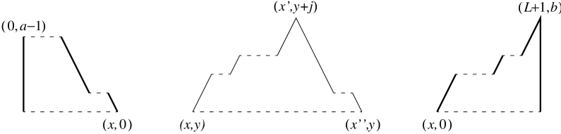
Figure 4: Typical examples of a left-boundary, bulk and right-boundary particle. The charges of the particles are $(a-1)/2$, $j$ and $b/2$, respectively.

With the above set of definitions we now give a prescription to divide each restricted lattice path into particles. This will be done by giving an algorithm that divides a complex into a particle and several smaller complexes. Each of these new complexes is either a particle or is again divided into a particle and yet smaller complexes. This procedure is continued until the entire complex is divided into particles. Since each lattice path can trivially be divided into complexes, this gives a procedure to divide any restricted lattice path into particles.

(0)

Draw a dashed line along the $x$-axis from $(0,0)$ to $(L+1,0)$, and draw bold lines from $(0,0)$ to $(0,a-1)$ and $(L+1,0)$ to $(L+1,b)$. This divides each restricted lattice path into a left-boundary complex, a right-boundary complex and a number of bulk complexes. For the restricted lattice path of Fig. 1, we for example get 4 complexes, 2 of which are of bulk-type. If $a=1$, the left-boundary complex is absent.

Now consider each of the complexes obtained above. If such a complex is a particle (in which case it is pure), we are done with it. If not, go to step (1) in case of a bulk complex and to (1_L) and (1_R) in case of a left- and right-boundary complex, respectively.

(1)

Start at the peak of the complex and move down to the right along the contour till the endpoint of the complex. When a local minimum is reached, i.e., the contour starts going up again, we draw a dashed line from this local minimum to the right until we cross the contour. At that point we move further down along the contour. If another minimum occurs we repeat the above, et cetera.

Repeat the above now moving to the left. That is, start from the peak of the complex and move down to the left till the origin of the complex. If a local minimum is reached we draw a dashed line to the left and continue our movement down when the dashed line intersects the contour.

As a result of the above step we have divided the complex into a particle (which is not pure) and several (at least one) smaller complexes. The peak and the baseline of the particle are the peak and the baseline of the original complex. Now go to (2).

(1_L)

Start from $(0,a-1)$. Move to the right of this point down along the contour of the complex till its endpoint. If a local minimum is reached (which could be the point $(0,a-1)$ itself), draw a dashed line from this minimum to the right, until the contour is crossed. At that point move further down along the contour. If another minimum occurs we repeat the above, et cetera.

As a result of the above step we have divided the left-boundary complex into a left boundary particle and several (at least one) smaller bulk complexes. To treat these smaller bulk complexes, go to (2).

(1_R)

Start from $(L+1,b)$. Move to the left of this point down along the contour of the complex till its endpoint. If a local minimum is reached, draw a dashed line from this minimum to the left until the contour is crossed. At that point move further down along the contour. If another minimum occurs repeat the above, et cetera.

As a result of the above step we have divided the right-boundary complex into a right-boundary particle and several (at least one) smaller bulk complexes. To treat these smaller bulk complexes, go to (2).

(2)

Scan each of the smaller bulk complexes. If such a complex is a bulk particle (in which case it is pure), we are done with it. If not repeat step (1) for this complex.

We note that the above procedure converges, since the number of local maxima of a restricted lattice path is finite. In Fig. 5, we have carried out the procedure for the restricted lattice path of Fig. 1, thereby identifying the corresponding configuration of particles.

Figure 5: The particle configuration corresponding to the restricted lattice path of Fig. 1.

Thanks to the above algorithm, each restricted lattice path in rlp$(0,r)$ can now be viewed as a particle configuration. In particular, since the maximal height of a path is $r-2$, we have bulk particles of charge 1 up to $r-2$, as well as a left-boundary particle of charge $(a-1)/2$ and a right-boundary particle of charge $b/2$. The contour of a bulk particle of charge $j$ consists of $j$ up and $j$ down steps, the contour of a left-boundary particle of $a-1$ down steps and the contour of a right-boundary particle of $b$ up steps. Letting $n_{j}$ denote the number of bulk particles of charge $j$, we thus have the completeness relation

$$a+b-1+2\sum_{j=1}^{r-2}j\,n_{j}=L+1.$$ (3.8)

Using this relation, $n_{r-2}$ can be computed given the occupation numbers $n_{1},\ldots,n_{r-3}$. For this reason (and anticipating things to come), we define the column vector $\vec{n}=\,^{T}(n_{1},\ldots,n_{r-3})$, and when we say “a restricted lattice path has particle content $C=\vec{n}\,$”, we mean by this the particle content $C=\{n_{1},\ldots,n_{r-2}\}$ subject to the restriction (3.8).

Having associated a configuration of particles with each path in rlp$(0,r)$, we define rlp$(\vec{n})$ as the subset of paths in rlp$(0,r)$, with particle content $\vec{n}$. This puts us in a position to properly define what we mean by the Fermi-gas partition function as introduced in (3.6),

$$Z(C;a,b)=Z(\vec{n};a,b)=\sum_{\mbox{\scriptsize rlp}(\vec{n})}\mbox{e}^{\;\displaystyle-\beta\sum_{j=1}^{L}E(j)},$$ (3.9)

with energy function defined in (3.2).

So far, we have repeatedly used the term Fermi-gas, without any clear motivation. Clearly, we have defined all allowed configurations of our one-dimensional system of charged particles, as well its Hamiltonian or energy function, but the actual nature of the system remains rather elusive. However, in our actual computation of $Z$, in the next subsection, it turns out to be expedient to define rules of motion that allow one to obtain any configuration with content $\vec{n}$ from a given so-called minimal configuration with the same content. These rules of motion have a clear fermionic character, in that particles of the same charge cannot exchange position, unlike particles of different charge.

3.3 Computation of $Z(\vec{n};a,b)$.

In this section we compute the partition function of the one-dimensional Fermi-gas. Throughout the section we assume the particle content to be $\vec{n}$.

To compute the sum over all particle configurations, we first select a particular configuration called the minimal configuration. It will be defined purely graphically.

Definition 7

The configuration shown in Fig. 6 is called the minimal configuration. Here each bulk particle of charge $j$ should be repeated $n_{j}$ times, i.e.,

Note that in the minimal configuration

• All (bulk) particles are positioned as much to the right and up as possible, the baseline of the particles of charge $j$ having $y$-coordinate equal to $\min(b-1,r-j-2)$.

• The particles are positioned in order of decreasing charge.

• Apart from the right-boundary particle, all particles are pure.

Figure 6: The restricted lattice path corresponding to the minimal configuration of particles. Here each bulk particle of charge $j$ has to be copied $n_{j}$ times. The dashed lines are the baselines of the particles.

3.3.1 Contribution of the minimal configuration

To compute the weight of the minimal configuration, we use that the energy $E_{j}(x)$ of a pure bulk particle of charge $j$, with origin at position $x$ and endpoint at position $x+2j$, is given by

$$E_{j}(x)=\frac{1}{2}\;\sum_{{k=1\atop k\neq j}}^{2j-1}(k+x)=(j+x)(j-1).$$ (3.10)

Similarly, we get for the energy $E_{a}$ of the pure left-boundary particle with charge $(a-1)/2$,

$$E_{a}=\frac{1}{4}(a-1)(a-2).$$ (3.11)

A bit more work is required to obtain the energy $E_{b}$ of the right-boundary particle with charge $b$, since its contour is broken into $b$ segments all of length 1. Summing up the $b$ different contributions leads to

$$E_{b}=\frac{1}{4}(b-1)(2a+b-2)+\sum_{j=r-b}^{r-2}j(b-r+j+1)n_{j}.$$ (3.12)

Using the above three results, we compute the energy of the minimal configuration as

$$E_{\min} = E_{a}+E_{b}+\sum_{j=1}^{r-2}\sum_{\ell=1}^{n_{j}}E_{j}\biggl{(}a-2+\min(b,r-j-1)+2j(\ell-1)+2\sum_{k=j+1}^{r-2}k\,n_{k}\biggr{)}$$

$$= \sum_{j=1}^{r-2}(j-1)n_{j}\biggl{(}j\,n_{j}+2\sum_{k=j+1}^{r-2}k\,n_{k}\biggr{)}+(a+b-2)\sum_{j=1}^{r-2}(j-1)n_{j}$$

$$+\sum_{j=r-b}^{r-2}(b-r+j+1)n_{j}+\frac{1}{4}(a-1)(a-2)+\frac{1}{4}(b-1)(2a+b-2).$$

To simplify this expression, we eliminate $n_{r-3}$ using the completeness relation (3.8). This yields

$$E_{\min}=\sum_{j=1}^{r-3}\left(\sum_{k=1}^{j}\frac{k(r-j-2)}{r-2}+\sum_{k=j+1}^{r-3}\frac{j(r-k-2)}{r-2}\right)n_{j}\,n_{k}$$

$$\qquad-\left(\sum_{j=1}^{r-b-1}\frac{j(b-1)}{r-2}+\sum_{j=r-b}^{r-3}\frac{(r-b-1)(r-j-2)}{r-2}+L\sum_{j=1}^{r-3}\frac{r-j-2}{r-2}\right)n_{j}$$

$$\qquad+\>\frac{L^{2}(r-3)+2L(b-1)-(a-1)(r-a-1)+(b-1)(r-b-1)}{4(r-2)}.$$

We now recall the definition of the inverse Cartan matrix of the Lie algebra A_r-3,

$$C^{-1}_{j,k}=\left\{\begin{array}[]{cc}\displaystyle\frac{k(r-j-2)}{r-2}&k\leq j\\ \displaystyle\frac{j(r-k-2)}{r-2}&k\geq j.\end{array}\right.$$ (3.15)

Using this, we finally obtain

Lemma 1

The energy of the minimal configuration is given by

$$E_{\min}=\sum_{j,k=1}^{r-3}\left(n_{j}-\frac{L}{2}\,\delta_{j,1}-\frac{1}{2}\,\delta_{j,r-b-1}-\frac{1}{2}\,\delta_{j,r-a-1}\right)C^{-1}_{j,k}$$ (3.16)

$$\qquad\qquad\qquad\qquad\qquad\times\left(n_{k}-\frac{L}{2}\,\delta_{k,1}-\frac{1}{2}\,\delta_{k,r-b-1}+\frac{1}{2}\,\delta_{k,r-a-1}\right).$$

3.3.2 Contribution of the non-minimal configurations

To compute the contribution to the partition function of the other configurations, we define rules of motion which generate all non-minimal configurations from the minimal one. These rules break up into several different elementary moves as follows.

Definition 8

Let $X=\{(x_{1},y_{1}),(x_{2},y_{2}),(x_{3},y_{3}),(x_{4},y_{4})\}$ denote a sequence of four points on the contour of a configuration, each pair of consecutive points connected straight lines, such that the contour in between $(x_{1},y_{1})$ and $(x_{4},y_{4})$ does not belong to a boundary particle. We may then replace this sequence by a new sequence of four points as follows.

move $L_{u}$:

If $y_{4}\leq y_{2}<y_{3}<y_{1}$,

$\qquad\qquad\qquad\quad L_{u}(X)=\{(x_{1},y_{1}),(x_{2}-1,y_{2}+1),(x_{3}-1,y_{3}+1),(x_{4},y_{4})\}$.

move $R_{d}$:

If $y_{4}<y_{2}<y_{3}\leq y_{1}$,

$\qquad\qquad\qquad\quad R_{d}(X)=\{(x_{1},y_{1}),(x_{2}+1,y_{2}-1),(x_{3}+1,y_{3}-1),(x_{4},y_{4})\}$.

move $L_{d}$:

If $y_{1}<y_{3}<y_{2}\leq y_{4}$,

$\qquad\qquad\qquad\quad L_{d}(X)=\{(x_{1},y_{1}),(x_{2}-1,y_{2}-1),(x_{3}-1,y_{3}-1),(x_{4},y_{4})\}$.

move $R_{u}$:

If $y_{1}\leq y_{3}<y_{2}<y_{4}$,

$\qquad\qquad\qquad\quad R_{u}(X)=\{(x_{1},y_{1}),(x_{2}+1,y_{2}+1),(x_{3}+1,y_{3}+1),(x_{4},y_{4})\}$.

Besides these “bulk-type” moves we need some special boundary moves.

Definition 9

Let $X=\{(x_{1},y_{1}),(x_{2},y_{2}),(x_{3},y_{3}),(x_{4},y_{4})\}$ be four points on the contour of a configuration, each pair of consecutive points connected by a straight line. We may then replace $X$ as follows.

move $L^{\prime}_{u}$:

Let $(x_{1},y_{1})=(x_{2}-1,y_{2}+1)$. If $y_{2}=y_{4}<r-2$ and the contour between the first two points belongs to the left-boundary particle,

$\qquad\qquad L^{\prime}_{u}(X)=\{(x_{2}-1,y_{2}+1),(x_{3}-1,y_{3}+1),(x_{4}-1,y_{4}+1),(x_{4},y_{4})\}$,

where the contour between the last two points belongs to the left-boundary particle.

move $R^{\prime}_{d}$:

Let $(x_{4},y_{4})=(x_{3}+1,y_{3}-1)$. If $y_{1}=y_{3}<2$ and the contour between the last two points belongs to the left-boundary particle,

$\qquad\qquad R^{\prime}_{d}(X)=\{(x_{1},y_{1}),(x_{1}+1,y_{1}-1),(x_{2}+1,y_{2}-1),(x_{3}+1,y_{3}-1)\}$,

where the contour between the last two points belongs to the left-boundary particle.

move $L^{\prime}_{d}$:

Let $(x_{1},y_{1})=(x_{2}-1,y_{2}-1)$. If $y_{2}=y_{4}<y_{3}$ and the contour between the first two points belongs to the right-boundary particle,

$\qquad\qquad L^{\prime}_{d}(X)=\{(x_{2}-1,y_{2}-1),(x_{3}-1,y_{3}-1),(x_{4}-1,y_{4}-1),(x_{4},y_{4})\}$,

where the contour between the last two points belongs to the right-boundary particle.

move $R^{\prime}_{u}$:

Let $(x_{4},y_{4})=(x_{3}+1,y_{3}+1)$. If $y_{1}=y_{3}<y_{2}<r-2$, $y_{3}<b-1$ and the contour between the last two points belongs to the right-boundary particle,

$\qquad\qquad R^{\prime}_{u}(X)=\{(x_{1},y_{1}),(x_{1}+1,y_{1}+1),(x_{2}+,y_{2}+1),(x_{3}+1,y_{3}+1)\}$,

where the contour between the first two points belongs to the right-boundary particle.

For the graphical interpretation of this long list of moves, see Fig. 7.

Figure 7: (a) The moves $L_{u}$ and $R_{u}$. (b) The moves $L_{d}$ and $R_{u}$. (c) The moves $L_{u}^{\prime}$ and $R_{u}^{\prime}$. (d) The moves $L_{d}^{\prime}$ and $R_{u}^{\prime}$.

To fully appreciate these moves, we list its main characteristics in several lemmas, which are at the core of our fermionic computation of the one-dimensional configuration sums.

Lemma 2

The elementary moves are reversible. That is, if there is a move of type $M_{s}^{p}$ from a configuration $C$ to a configuration $C^{\prime}$, then there is a move of type $\bar{M}_{\bar{s}}^{p}$ from $C^{\prime}$ to $C$. Here $M=L$ or $R$, $s=u$ or $d$, $p=\quad,\,^{\prime}$ or ^′′ and $\bar{R}=L$, $\bar{L}=R$, $\bar{u}=d$ and $\bar{d}=u$.

Proof: Let us show this for $L_{u}$. The other moves follow in similar manner. Let $X$ be a sequence of four extrema as in definition 8, satisfying $y_{4}\leq y_{2}<y_{3}<y_{1}$. Hence we can carry out $L_{u}$ to obtain $X^{\prime}=L_{u}(X)=\{(x^{\prime}_{1},y^{\prime}_{1}),(x^{\prime}_{2},y^{\prime}_{2}),(x^{\prime}_{3},y^{\prime}_{3}),(x^{\prime}_{4},y^{\prime}_{4})\}$. From the definition of the move $L_{u}$, we find that $y_{4}^{\prime}\leq y_{2}^{\prime}-1<y_{3}^{\prime}-1<y_{1}$. We rewrite this to obtain $y_{4}^{\prime}<y_{2}^{\prime}<y_{3}^{\prime}\leq y_{1}$ and hence we can carry out the move $R_{d}$ to obtain $R_{d}(X^{\prime})=X$. $\Box$

Lemma 3

The moves leave the particle content $\vec{n}$ fixed.

Proof: This follows immediately from the graphical representation of the moves shown in Fig. 7, where the dashed lines represent the baselines of the pure particles being moved. Note here that the graphical representations of the moves $R_{u}$ and $L_{d}$ are the generic cases. Performing a move of type $R_{u}$ to a sequence $X$ as defined in definition 8, with $y_{2}=y_{4}-1$, may lead to a “jump” of the baseline. A similar thing may happen when performing a move of type $L_{d}$ to a sequence with $y_{2}=y_{4}$:

$$\centerline{\hbox{\epsfbox{jump.ps}}}\Box$$

Lemma 4

Given the minimal configuration, we cannot make any of the $R$-type moves.

Proof: We can only make moves of type $R_{d}$ if we have a sequence of $X$ as in definition 8, with $y_{4}<y_{2}$. Clearly this does not occur. We can only make moves of type $R_{u}$ if we have a sequence $X$, with $y_{2}<y_{4}$. Again this does not occur. We cannot make a move of type $R^{\prime}_{d}$ since the left-boundary particle is in its pure form. Finally, we cannot make a move of type $R^{\prime}_{u}$ since all particles of charge $j\geq r-b-1$ have their peak at $y=r-2$, and all particles of charge $j\leq r-b-1$ have their endpoint at $y=b-1$. $\Box$

Lemma 5

If a configuration is not the minimal one, we can always make a move of type $R$.

Proof: By construction the minimal configuration is the only configuration that does not meet any of the conditions required for one of the $R$-type moves. In particular, all maxima (apart from the initial point of the path) are of decreasing order and all minima of increasing order. This completely fixes the path. If one of these two properties is broken somewhere along the path, we can always make an $R$-type move. $\Box$

These first four lemmas can be combined to give the following proposition:

Proposition 1

All non-minimal paths are generated by moves of type $L$ from the minimal configuration. All non-minimal configurations can be reduced to the minimal configuration by moves of type $R$.

Having established the above proposition, we can perform the actual calculation of the generation function $\cal C$ of the moves of type $L$. Again we prepare some lemmas to obtain the desired result.

Lemma 6

Each move of type $L$ generates a factor $q$.

Proof: We show this for the typical case of move $L_{u}$. The total energy $E$ of a sequence of extrema $X$ is

$$E=\sum_{{j=x_{1}+1\atop j\neq x_{2},x_{3}}}^{x_{4}-1}j.$$ (3.17)

Similarly, the energy $E^{\prime}$ of the sequence $X^{\prime}=L_{u}(X)$ is

$$E=\sum_{{j=x_{1}+1\atop j\neq x_{2}-1,x_{3}-1}}^{x_{4}-1}j.$$ (3.18)

Hence we find

$$\mbox{e}^{-\beta(E^{\prime}-E)}=q^{E^{\prime}-E}=1.\qquad\quad\Box$$ (3.19)

In the following it will be convenient to label the bulk particles in the minimal configuration, letting $p_{j,\ell}$ denote the $\ell$-th particle of charge $j$, counted from the left. To now generate all non-minimal configurations, we give an ordering for carrying out the moves of type $L$.

• The particle $p_{j,\ell}$ is moved to the left using moves of type $L$, prior to any of the particles $p_{k,m}$, with $k\leq j$, and with $m>\ell$ if $k=j$.

Assuming this order (which will be justified later), we have

Lemma 7

The maximal number of $L$-type moves $p_{j,1}$ can make is

$$m_{j}=2\sum_{k=j+1}^{r-2}(k-j)\,n_{k}+\min(a-1,r-j-2)+\min(b-1,r-j-2).$$ (3.20)

Proof: We proof this lemma in two steps. In the first step (3.20) is shown to be true for the minimal configuration, and in the second step it is shown that $m_{j}$ is invariant under having moved the particles $p_{k,m}$, with $k>j$, prior to $p_{j,1}$.

Let us start to calculate the number of $L$-type moves needed to exchange the position of two particles of charge $k$ and $j$, $k>j$, with $j$ positioned immediately to the right of $k$. In such a configuration of two particles we have a sequence $X=\{(x_{1},y_{1}),\ldots,(x_{5},y_{5})\}$ of points connected by straight lines, with $y_{1}=y_{3}=y_{5}$ and $y_{2}=k$ and $y_{4}=j$. From these conditions it follows that move $L_{u}$ can be carried out $k-j$ times to the sequence $\{(x_{2},y_{2}),\ldots,(x_{5},y_{5})\}$. This gives a new sequence $X^{\prime}=\{(x^{\prime}_{1},y^{\prime}_{1}),\ldots,(x^{\prime}_{5},y^{\prime}_{5})\}$, with $y^{\prime}_{1}=y^{\prime}_{5}$, $y^{\prime}_{2}=y^{\prime}_{4}=k$ and $y^{\prime}_{3}=k-j$. From these conditions it follows that move $L_{d}$ can be carried out $k-j$ times to the sequence $\{(x^{\prime}_{1},y^{\prime}_{1}),\ldots,(x^{\prime}_{4},y^{\prime}_{4})\}$. This gives the final sequence $X^{\prime\prime}=\{(x^{\prime\prime}_{1},y^{\prime\prime}_{1}),\ldots,(x^{\prime\prime}_{5},y^{\prime\prime}_{5})\}$, with $y^{{}^{\prime\prime}}_{1}=y^{{}^{\prime\prime}}_{3}=y^{{}^{\prime\prime}}_{5}$, $y^{{}^{\prime\prime}}_{2}=j$ and $y^{{}^{\prime\prime}}_{4}=k$. The total number of moves carried out is therefore $2(k-j)$. Since in the minimal configuration there are $n_{k}$ particles of charge $k$ to the left of $p_{j,1}$, this gives a total contribution $\sum_{k=j+1}^{r-2}(k-j)\,n_{k}$. Apart from this, we encounter the situation where immediately to the left of $p_{j,1}$ we have a segment of the right-boundary particle. In such an instant we can perform $L^{\prime}_{d}$, moving $p_{j,1}$ one step down. By construction of the minimal configuration, this occurs $\min(b-1,r-j-2)$ times. Finally, after having descended all the way down and having exchanged position with all particles of charge $>j$, $p_{j,1}$ is positioned immediately to the right of the left-boundary particle. It can then move up exactly $\min(a-1,r-j-2)$ times using move $L^{\prime}_{u}$. Adding up all the contributions gives (3.20).

To see that (3.20) is unaltered by first having moved some (or all) particles of charge greater than $j$, consider a sequence of four points $X=\{(x_{1},y_{1}),(x_{2},y_{2}),(x_{3},y_{3}),(x_{4},y_{4})\}$ connected by straight lines. First, let $y_{1}>y_{2}<y_{3}>y_{4}$ and let $p_{j,1}$ be positioned immediately to the right of the sequence, i.e., the origin of $p_{j,1}$ is at $(x_{4},y_{4})$. Also, let the contour between the first two points not belong to the left-boundary particle. The total number of $L$-type steps $p_{j,1}$ can make is then $(y_{3}-y_{4}-j)+(y_{3}-y_{2}-j)+(y_{1}-y_{2}-j)=x_{4}-x_{1}-3j$, which is independent of the positions of the points $(x_{2},y_{2})$ and $(x_{3},y_{3})$. Hence carrying out any moves to $X$ does not change the number of moves $p_{j,1}$ can make relative to $X$. If the contour between the first two point does belong to the left-boundary particle, this is changed to $x_{4}-x_{1}-3j+r-2-\min(r-2-j,y_{1})$ which is still independent of the relative positions of $(x_{2},y_{2})$ and $(x_{3},y_{3})$. Second, let $y_{1}<y_{2}>y_{3}<y_{4}$ and let $p_{j,1}$ be positioned immediately to the left of the sequence, i.e., the endpoint of $p_{j,1}$ is at $(x_{1},y_{1})$. Also, let the contour between the last two points not belong to the left-boundary particle. The total number of $R$-type steps $p_{j,1}$ can make is then $(y_{2}-y_{1}-j)+(y_{2}-y_{3}-j)+(y_{4}-y_{3}-j)=x_{4}-x_{1}-3j$, which is independent of the positions of the points $(x_{2},y_{2})$ and $(x_{3},y_{3})$. Thanks to reversibility, the number of $L$-type moves $p_{j,1}$ can make relative to $X$ is also $x_{4}-x_{3}-3j$. If the contour between the last two point does belong to the right-boundary particle, this again chances by a term independent of the detailed positions of $(x_{2},y_{2})$ and $(x_{3},y_{3})$. $\Box$

Lemma 8

The maximal number of $L$-type moves $p_{j,\ell}$ can make is $k_{j,\ell-1}$, with $k_{j,\ell-1}$ the actual number of steps taken by $p_{j,\ell-1}$

At last!, we finally encountered the fermionic nature of our lattice-gas. Proof: Assume $p_{j,\ell-1}$ has made $k_{j,\ell-1}$ moves. Obviously, (before) the first $k_{j,\ell-1}$ moves, $p_{j,\ell}$ “sees” the same contour immediately to its left as $p_{j,\ell-1}$ did, when carrying out its leftward motion. Since $p_{j,\ell-1}$ and $p_{j,\ell}$ are identical particles, $p_{j,\ell}$ can thus carry out at least $k_{j,\ell-1}$ moves. Let $p_{j,\ell}$ indeed carry out $k_{j,\ell-1}$ moves. After that we encounter the situation of two pure particles of charge $j$, with endpoint of the first being origin of the next. The right-most of the two can neither carry out $L_{u}$, nor $L_{d}$, since (in the notation of definition 8) $y_{1}=y_{3}$. $\Box$

We note that the above two lemmas justify the chosen ordering of carrying out the leftward moves. First of all, by lemma 8 it follows that we indeed have to move $p_{j,\ell-1}$ before $p_{j,\ell}$. Furthermore, we have to move $p_{k,m}$ before $p_{j,\ell}$, $k>j$ since the elementary moves only allow for leftward motion of pure particles, see Fig. 7. Finally we have seen in the proof of lemma 7 that the number of moves the particles of charge $j$ can make is independent of the actual configuration of particles of charge $>j$.

Lemma 9

The contribution to the generating function $C$ of the particles of charge $j$, is given by $\cal C$, is given by

$${\cal C}_{j}=\biggl{[}{m_{j}+n_{j}\atop n_{j}}\biggr{]}.$$ (3.21)

Proof: From the lemmas 6, 7 and 8 we get (dropping the subscripts $j$ in the $k$-variables)

$${\cal C}_{j}=\sum_{k_{1}=0}^{m_{j}}\sum_{k_{2}=0}^{k_{1}}\ldots\sum_{k_{n_{j}}=0}^{k_{n_{j}-1}}q^{k_{1}+k_{2}+\cdots+k_{n_{j}}}.$$ (3.22)

We can (re)interpret this sum as the generating function of all partitions with largest part less or equal to $m_{j}$ and number of parts less or equal to $n_{j}$. Thus we get (3.21), see e.g., ref. [9].

Combining the above lemma with lemma 1, we can state our second proposition as

Proposition 2

The partition function of the one-dimensional Fermi-gas is given by

$$Z(\vec{n};a,b)=q^{E_{\min}}\prod_{j=1}^{r-3}{\cal C}_{j}=q^{E_{\min}}\prod_{j=1}^{r-3}\biggl{[}{m_{j}+n_{j}\atop n_{j}}\biggr{]},$$ (3.23)

with $E_{\min}$ given by (3.16) and $m_{j}$ by (3.20).

To recast this result into a simpler from, we eliminate the $n$-variables in favour of the $m$-variables. To do so we use the simple formulae

$$-\min(p,q-1)+2\,\min(p,q)-\min(p,q+1)=\delta_{p,q}\qquad\>p,q-1\geq 0$$

$$-\min(p,q-1)+2\,\min(p,q)=p+\delta_{p,q}\qquad\qquad\quad\qquad 0\leq p\leq q+1$$ (3.24)

to get

$$-m_{j-1}+2m_{j}-m_{j+1}=L\,\delta_{j,1}+\delta_{j,r-a-1}+\delta_{j,r-b-1}-2n_{j}\qquad j=1,\ldots,r-3$$ (3.25)

with $m_{0}=m_{r-2}=0$. To obtain the $j=1$ case of the above equation we made use of the completeness relation (3.8). Introducing the $(r-3)$-dimensional vectors $\vec{m}$ and $\vec{\mbox{e}}_{j}$ with entries $(\vec{m})_{j}=m_{j}$ and $(\vec{\mbox{e}}_{j})_{k}=\delta_{j,k}$, we can rewrite (3.25) as

$$\vec{n}=\frac{1}{2}\>(L\,\vec{\mbox{e}}_{1}+\vec{\mbox{e}}_{r-a-1}+\vec{\mbox{e}}_{r-b-1}-C\>\vec{m}).$$ (3.26)

Substituting this into equations (3.16) and (3.23), we arrive at the following simple result:

Proposition 3

The partition function of the Fermi-gas of content $\vec{n}$ reads

$$Z(\vec{n};a,b)=q^{\,{\textstyle{1\over 4}}\,\vec{m}^{T}C\,\vec{m}-{\textstyle{1\over 2}}\,m_{r-a-1}}\prod_{j=1}^{r-3}\biggl{[}{\frac{1}{2}({\cal I}\,\vec{m}+L\,\vec{\mbox{e}}_{1}+\vec{\mbox{e}}_{r-a-1}+\vec{\mbox{e}}_{r-a-1})_{j}\atop m_{j}}\biggr{]},$$ (3.27)

whth, $\vec{m}$ obtained through equation (3.26).

3.4 Computation of $\Xi_{L}(a,b)$.

Having computed the partition function of our Fermi-gas, it is only a trivial step to obtain the grand-canonical partition function $\Xi_{L}(a,b)$, defined in (3.6). In particular

$$\Xi_{L}(a,b)=\sum_{\vec{n}}Z(\vec{n};a,b).$$ (3.28)

Since our final result (3.27) for $Z$ is entirely expressed through the $m$-variables, it is natural to also express the above sum over $\vec{n}$ in terms of a sum over $\vec{m}$. From $(\ref{mj})$, and the fact that the occupation numbers $n_{j}$ cannot be negative, we get

$$m_{j}=\min(a-1,r-j-2)+\min(b-1,r-j-2)+2\>\mbox{\sf Z}\mbox{\sf Z}\,_{\geq 0}\qquad j=1,\ldots,r-3.$$ (3.29)

Hence we obtain the grand-canonical partition function as

$$\Xi_{L}(a,b)=\left.\sum_{\vec{m}}\right.^{(0)}q^{\,{\textstyle{1\over 4}}\,\vec{m}^{T}C\,\vec{m}-{\textstyle{1\over 2}}\,m_{r-a-1}}\prod_{j=1}^{r-3}\biggl{[}{\frac{1}{2}({\cal I}\,\vec{m}+L\,\vec{\mbox{e}}_{1}+\vec{\mbox{e}}_{r-a-1}+\vec{\mbox{e}}_{r-a-1})_{j}\atop m_{j}}\biggr{]},$$ (3.30)

where the $(0)$ in the sum over $\vec{m}$ denotes the restriction (3.29).

3.5 Computation of $X_{L}(a,b)$.

To finally obtain the one-dimensional configuration sum $X_{L}(a,b)$, we have to carry out the sum (3.5), where we recall that $\Xi_{L}(a,b):=\Xi_{L}(a,b,0,r)$.

To get the expression for $\Xi_{L}(a-\mu,b-\mu,0,r-\mu)$, we have to make the substitutions $a\to a-\mu$, $b\to b-\mu$ and $r\to r-\mu$ in (3.30). This exactly gives back (3.30) apart from the fact that the restriction on the sum changes to

$$m_{j}=\left\{\begin{array}[]{ll}\min(a-1,r-j-2)&\\ \quad+\min(b-1,r-j-2)-2\mu+2\>\mbox{\sf Z}\mbox{\sf Z}\,_{\geq 0}&j=1,\ldots,r-\mu-3\\ 0&j=r-\mu-2,\ldots,r-3.\end{array}\right.$$ (3.31)

Denoting this restriction as $(\mu)$, we can write

$$X_{L}(a,b)=\sum_{\mu=0}^{\min(a,b)-1}\left.\sum_{\vec{m}}\right.^{(\mu)}q^{\,{\textstyle{1\over 4}}\,\vec{m}^{T}C\,\vec{m}-{\textstyle{1\over 2}}\,m_{r-a-1}}\prod_{j=1}^{r-3}\biggl{[}{\frac{1}{2}({\cal I}\,\vec{m}+L\,\vec{\mbox{e}}_{1}+\vec{\mbox{e}}_{r-a-1}+\vec{\mbox{e}}_{r-a-1})_{j}\atop m_{j}}\biggr{]}.$$ (3.32)

Combining the sum over $\vec{m}$ restricted to $(\mu)$ and the sum over $\mu$, gives

$$X_{L}(a,b)=\left.\sum_{\vec{m}}\right.^{{}^{\prime}}q^{\,{\textstyle{1\over 4}}\,\vec{m}^{T}C\,\vec{m}-{\textstyle{1\over 2}}\,m_{r-a-1}}\prod_{j=1}^{r-3}\biggl{[}{\frac{1}{2}({\cal I}\,\vec{m}+L\,\vec{\mbox{e}}_{1}+\vec{\mbox{e}}_{r-a-1}+\vec{\mbox{e}}_{r-a-1})_{j}\atop m_{j}}\biggr{]},$$ (3.33)

with the prime denoting yet another restriction,

$$m_{j}\equiv\min(a-1,r-j-2)+\min(b-1,r-j-2)\qquad j=1,\ldots,r-3.$$ (3.34)

Unfortunately, we have not found an elegant way to prove this simplification and we defer it till the appendix.

To rewrite the above form of the restriction, in the form conjectured in refs. [5, 10], we note the identity

$$\begin{array}[]{rcccccccc}\min(p,q)&\equiv&\delta_{p+1,q}&+&\delta_{p+3,q}&+&\delta_{p+5,q}&+&\ldots\\ &+&\delta_{1,q}&+&\delta_{3,q}&+&\delta_{5,q}&+&\ldots\;,\end{array}$$ (3.35)

for $p,q\geq 0$. Using this twice, once setting setting $p=a-1$ and $q=r-j-2$, and once setting $p=b-1$ and $q=r-j-2$, we get $m_{j}\equiv(\vec{Q}_{a,b})_{j}$, with $\vec{Q}_{a,b}$ given by (2.2).

We can thus conclude this section formulating our main result as a theorem.

Theorem 1

For all $a=1,\ldots,r-1$, $b=1,\ldots,r-2$ and $L-|a-b|\in 2\,\>\mbox{\sf Z}\mbox{\sf Z}\,_{\geq 0}$, the one-dimensional configuration sum (1.5), is given by

$$X_{L}(a,b)=\sum_{\vec{m}\equiv\vec{Q}_{a,b}}q^{\,{\textstyle{1\over 4}}\,\vec{m}^{T}C\,\vec{m}-{\textstyle{1\over 2}}\,m_{r-a-1}}\prod_{j=1}^{r-3}\biggl{[}{\frac{1}{2}({\cal I}\,\vec{m}+L\,\vec{\mbox{e}}_{1}+\vec{\mbox{e}}_{r-a-1}+\vec{\mbox{e}}_{r-b-1})_{j}\atop m_{j}}\biggr{]},$$

where $\vec{Q}_{a,b}$ is given by (2.2).

4 Bosonic solution of the ABF model

In this section we recall the method for computing the sum (1.5) to obtain (up to a prefactor) the right-hand side of Melzer’s identities (2.1). This alternative approach to the sum (1.5) is the one originally taken by Andrews, Baxter and Forrester [12] and is given here mainly for reasons of completeness.

As a first step we introduce a function $Y_{L}(a,b)$ defined exactly as $X_{L}(a,b)$ in (1.5), but with $\sigma_{L+1}=b-2$ instead of $\sigma_{L+1}=b$. We can then immediately infer the recurrence relations

$$X_{L}(a,b) = \,Y_{L-1}(a,b+1)+q^{L/2}X_{L-1}(a,b-1)\quad\qquad 1\leq b\leq r-2$$ (4.1)

$$Y_{L}(a,b) = X_{L-1}(a,b-1)+q^{L/2}\,Y_{L-1}(a,b+1)\quad\qquad 2\leq b\leq r-1,$$ (4.2)

subject to the initial and boundary conditions

$$X_{0}(a,b)=Y_{0}(a,b)=\delta_{a,b}$$ (4.3)

$$X_{L}(a,0)=Y_{L}(a,r)=0.$$ (4.4)

To state the solution to these equations, we quote the following theorem established by Andrews, Baxter and Forrester [12]:

Theorem 2

For $L\geq 0$, $1\leq a,b,c\leq r-1$, $c=b\pm 1$, $L+a-b\equiv 0$, let $X_{L}(a,b,c):=X_{L}(a,b)$ if $c=b+1$ and $X_{L}(a,b,c):=Y_{L}(a,b)$ if $c=b-1$. Then

$$X_{L}(a,b,c)=q^{(a-b)(a-c)/4}\sum_{j=-\infty}^{\infty}\left\{q^{j\bigl{(}r(r-1)j+r(b+c-1)/2-(r-1)a\bigr{)}}\left[{\textstyle{L\atop\frac{1}{2}(L+a-b)-rj}}\right]\right.$$ (4.5)

$$\left.\qquad\qquad\qquad\qquad\qquad\qquad\;-q^{\bigl{(}(r-1)j+(b+c-1)/2\bigr{)}\bigl{(}rj+a\bigr{)}}\left[{\textstyle{L\atop\frac{1}{2}(L-a-b)-rj}}\right]\right\}.$$

To proof this, we note that (4.5) satisfies (4.1), thanks to

$$\biggl{[}{N\atop m}\biggr{]}=\biggl{[}{N-1\atop m-1}\biggr{]}+q^{m}\biggl{[}{N-1\atop m}\biggr{]}.$$ (4.6)

Similarly, the proof that (4.5) satisfies (4.2) follows by application of

$$\biggl{[}{N\atop m}\biggr{]}=\biggl{[}{N-1\atop m}\biggr{]}+q^{N-m}\biggl{[}{N-1\atop m-1}\biggr{]}.$$ (4.7)

To show that the initial condition (4.3) holds, note (1.3) as well as the range of $a$ and $b$. This gives $j=0$ as the only non-vanishing term in the sum, and hence $X_{0}(a,b,c)=\delta_{a,b}$. Finally, $X_{L}(a,0)=0$ follows from (4.5) upon substitution of $b=0$, $c=1$ and making the change of variables $j\to-j$ in the first term withing the curly braces. Analogously, $Y_{L}(a,r)$ follows from (4.5) upon substituting $b=r$, $c=r-1$ and making the change of variables $j\to-j-1$ in the first term within the braces. $\Box$.

To obtain the desired expression for $X_{L}(a,b)$, we set $c=b+1$ in (4.5) yielding

$$X_{L}(a,b)=f_{a,b}^{-1}\sum_{j=-\infty}^{\infty}\left\{q^{j\bigl{(}r(r-1)j+rb-(r-1)a\bigr{)}}\left[{\textstyle{L\atop\frac{1}{2}(L+a-b)-rj}}\right]\right.$$ (4.8)

$$\left.\qquad\qquad\qquad\qquad\;-q^{\bigl{(}(r-1)j+b\bigr{)}\bigl{(}rj+a\bigr{)}}\left[{\textstyle{L\atop\frac{1}{2}(L-a-b)-rj}}\right]\right\}.$$

Combined with theorem 1 on page 1, this proves Melzer’s polynomial identities (2.1).

In conclusion to this section we make two remarks about the solution (4.8). First, the introduction of the auxiliary function $Y_{L}(a,b)$ could have been avoided, since from the definition (1.5) one can obtain recurrences that only involve the function $X_{L}(a,b)$. In particular,

$$X_{L}(a,b)=\left\{\begin{array}[]{ll}q^{L/2}X_{L-1}(a,b-1)+q^{(L-1)/2}X_{L-1}(a,b+1)&\\ \qquad\qquad\qquad\qquad\,+(1-q^{L-1})X_{L-2}(a,b)&b=1,\ldots,r-3\\ q^{L/2}X_{L-1}(a,b-1)+X_{L-2}(a,b)&b=r-2,\end{array}\right.$$ (4.9)

with the same conditions on $X_{L}(a,b)$ as in (4.3) and (4.4). The price to be paid for this is that, in order to show (4.8) solves these relations, we need double application of (4.6) and (4.7). Interestingly though, in terms of the fermionic left-hand side of (2.1), the recurrences (4.9) seem to be more natural, see e.g., ref. [11].

A second remark we wish to make is that like the fermionic result (2.1), also (4.8) has a nice interpretation in terms of restricted lattice paths. To see this, note that in order to obtain the generating function for the restricted lattice paths, we can first compute the generating function $G_{L}(\emptyset)$ of restricted lattice paths without the restriction $0\leq y\leq r-2$. Since all paths that go below $y=0$ and above $y=r-2$ have now incorrectly been included, we have to subtract the generating function $G_{L}(\downarrow)$ of paths that somewhere go below $y=0$, as well as the generating function $G_{L}(\uparrow)$ of paths that somewhere go above $y=r-2$. However, we are again in error, since paths that go below $y=0$ as well as above $y=r-2$ have been subtracted twice. To correct this we add $G_{L}(\downarrow,\uparrow)$ and $G_{L}(\uparrow,\downarrow)$, being the generating function of all paths that somewhere go above $y=r-2$ after having gone below $y=0$ and the generating function of all paths that somewhere go below $y=0$ after having gone above $y=r-2$. Again this is no good, and we keep continuing the process of adding and subtracting generating functions. In formula this reads

$$X_{L}(a,b)=\sum_{j\geq 0}\Bigl{\{}G_{L}(\underbrace{\downarrow\uparrow\cdots\downarrow\uparrow}_{2j})+G_{L}(\underbrace{\uparrow\downarrow\cdots\uparrow\downarrow}_{2j+2})-G_{L}(\underbrace{\downarrow\uparrow\cdots\uparrow\downarrow}_{2j+1})-G_{L}(\underbrace{\uparrow\downarrow\cdots\downarrow\uparrow}_{2j+1})\Bigr{\}},$$ (4.10)

with $G_{L}(\underbrace{\downarrow\uparrow\cdots\downarrow\uparrow}_{2j})$ the generating function of all lattice paths that contain a sequence of extrema $\{(x_{1},y_{1}),(x_{2},y_{2}),\ldots,(x_{2j},y_{2j})\}$, with $x_{j}>x_{k}$ for $j>k$, $y_{2k-1}<0$ and $y_{2k}>r-2$, and with the other generating functions defined similarly. Of course, since we consider paths of fixed, finite length, the above series only contains a finite number of nonzero terms. Computing the functions $G_{L}$, we obtain

$$G_{L}(\underbrace{\downarrow\uparrow\cdots\downarrow\uparrow}_{2j}) = f_{a,b}^{-1}\>q^{j\bigl{(}r(r-1)j-rb+(r-1)a\bigr{)}}\left[{\textstyle{L\atop\frac{1}{2}(L-a+b)-rj}}\right]$$

$$G_{L}(\underbrace{\uparrow\downarrow\cdots\uparrow\downarrow}_{2j}) = f_{a,b}^{-1}\>q^{j\bigl{(}r(r-1)j+rb-(r-1)a\bigr{)}}\left[{\textstyle{L\atop\frac{1}{2}(L+a-b)-rj}}\right]$$

$$G_{L}(\underbrace{\downarrow\uparrow\cdots\uparrow\downarrow}_{2j+1}) = f_{a,b}^{-1}\>q^{\bigl{(}(r-1)j+b\bigr{)}\bigl{(}rj+a\bigr{)}}\left[{\textstyle{L\atop\frac{1}{2}(L-a-b)-rj}}\right]$$ (4.11)

$$G_{L}(\underbrace{\uparrow\downarrow\cdots\downarrow\uparrow}_{2j+1}) = f_{a,b}^{-1}\>q^{\bigl{(}(r-1)(j+1)-b\bigr{)}\bigl{(}r(j+1)+a\bigr{)}}\left[{\textstyle{L\atop\frac{1}{2}(L+a+b)-r(j+1)}}\right],$$ (4.12)

for all $j\geq 0$. Substitution in (4.10) correctly reproduces the expression (4.8). We remark that the above described method for computing $X_{L}(a,b)$ is merely a rewording of the sieving technique developed by Andrews in the context of partition theory, see e.g., ref. [9]. For the details of the calculation leading to (4.11) we refer the reader to ref. [9], Chapter 9, and ref. [24].

5 Summary and discussion

In this paper we have, using the combinatorial technique developed in part I, computed all one-dimensional configuration sums of the $(r-1)$-state ABF model. In contrast to the earlier results of Andrews, Baxter and Forrester, our expressions are of so-called fermionic type, and provide a new proof of polynomial identities conjectured by Melzer. In the limit of an infinitely large lattice, these identities imply the fermionic expressions for the $\chi_{b,a}^{(r-1,r)}(q)$ Virasoro characters as conjectured by the Stony Brook group. Using the Andrews–Bailey construction, we also proved fermionic expressions for several non-unitary minimal Virasoro characters.

In conclusion to this paper we make a few comments. First, motivated by the ground breaking papers of the Stony Brook group [5, 19, 20, 25, 26], a vast literature has arisen containing numerous claims for identities of the Rogers–Ramanujan type [10,27-34]. We expect that our fermionic method for computing generating functions of restricted lattice paths can be applied to obtain proof of several of these conjectures. Other recently developed approaches towards either proof, or an increase of understanding, of Fermi-Bose character identities, can for e.g., be found in refs. [6,7,11,35-47].

A second remark is that in the $q=1$ limit, Melzer’s identities reduce to identities for the number of $L$-step paths on the A_r-1 Dynkin diagram, with fixed initial and final position. Viewed this way, it turns out that Melzer’s identities are in fact a special 1-dimensional case of polynomial identities for $q$-deformed path-counting on arbitrary $d$-dimensional cuboids. In the limit of infinitely long paths, these “cuboid” identities decouple into products of Virasoro character identities. The simplest example beyond Melzer’s case is the $q$-deformation of a path-counting formula on a “railroad” of length $r-3$, reading:

$$f_{a,b}\sum_{\vec{m}\equiv\vec{Q}_{a,b}}q^{\>{\textstyle{1\over 4}}\,\vec{m}^{T}C\>\vec{m}-{\textstyle{1\over 2}}\,m_{r-a-1}}\biggl{[}{L\atop m_{1}}\biggr{]}\prod_{j=2}^{r-3}\biggl{[}{\frac{1}{2}({\cal I}\,\vec{m}+\vec{\mbox{e}}_{r-a-1}+\vec{\mbox{e}}_{r-b-1})_{j}\atop m_{j}}\biggr{]}$$ (5.1)

$$=\sum_{j=-\infty}^{\infty}\left\{q^{j\big{(}r(r-1)j+rb-(r-1)a\big{)}}\left[{\textstyle{L\atop 2(r-1)j+b-a}}\right]_{2}-q^{\big{(}(r-1)j+b\big{)}\big{(}rj+a\big{)}}\left[{\textstyle{L\atop 2(r-1)j+b+a}}\right]_{2}\right\},$$

for $a,b=1,\ldots,r-2$ and $L\geq 0$. Here $\left[{\textstyle{N\atop m}}\right]_{2}$ are $q$-deformed trinomial coefficients defined as [48]

$$\biggl{[}{N\atop m}\biggr{]}_{2}=\sum_{k\geq 0}q^{k(k+m)}\biggl{[}{N\atop k}\biggr{]}\biggl{[}{N-k\atop k+m}\biggr{]}.$$ (5.2)

A discussion for the case of arbitrary cuboids will be presented elsewhere [49].

A final remark is that the result (1) proven in this paper has nice partition theoretical interpretations. One follows from the work of Andrews et al. [24], stating that the one-dimensional configuration sum $X_{L}(a,b)$ is the generating function of all partitions into at most ${\textstyle{1\over 2}}(L+a-b)$ parts, each part $\leq{\textstyle{1\over 2}}(L-a+b)$, such that the hook differences on the $(1-b)$-th diagonal are $\geq b-a+1$ and on the $(r-b-2)$-th diagonal $\leq b-a$. Another interpretation follows by viewing a restricted lattice path with total energy $E$ as a partition of $2E=\lambda_{1}+\lambda_{2}+\ldots+\lambda_{M}$, with $\lambda_{j}$ the $j$-th $x$-position counted from the right, where the path has no extremum. With this map from paths to partitions, $X_{L}(a,b;q^{2})$ is the generating function of partitions into parts $\lambda_{1},\lambda_{2},\ldots,\lambda_{M}$, with $\lambda_{M}<\ldots<\lambda_{2}<\lambda_{1}\leq L$, and

$$\begin{array}[]{l}1-b\leq u_{j}-d_{j}\leq r-b-2\qquad\quad\forall j=1,\ldots,M\\ u_{M}-d_{M}=a-b,\;a-b-1.\end{array}$$ (5.3)

Here $u_{j}$ is the number of parts $\lambda_{k}\equiv a-b+k$ for $k\leq j$ and $d_{j}$ is the number of parts $\lambda_{k}\not\equiv a-b+k$ for $k\leq j$.

Note added

After completing this manuscript we received a preprint by A. Schilling [50], in which (2.1) as well as (2.1) are proven as special cases of polynomial identities for finitized branching functions of the cosets

Appendix A Proof of equivalence of (3.32) and (3.33)

In this appendix we proof that (3.32) can be simplified to yield the final result (3.33) for the one-dimensional configuration sums.

The problem with this step is that the following statement turns out to be false:

$$\sum_{\mu=0}^{\min(a,b)-1}\left.\sum_{\vec{m}}\right.^{(\mu)}=\left.\sum_{\vec{m}}\right.^{{}^{\prime}},$$ (A.1)

where $(\mu)$ denotes the restriction (3.31) and the prime the restriction (3.34). In particular, the number of vectors $\vec{m}$ which are in accordance with the restriction (3.34) exceed the number over vectors $\vec{m}$ in accordance with the restriction (3.31) summed over $\mu$. What we will show now is that each of the additional $\vec{m}$’s allowed by the sum on the right-hand side gives a vanishing contribution.

Let us assume that $\min(a,b)=M+1$, so that we have $M+1$ terms in the sum over $\mu$. Let us further define $S_{\mu}$ as the set of $\vec{m}$-vectors allowed by the restriction (3.31). In other words, $\vec{m}\in S_{\mu}$ if

$$\left\{\begin{array}[]{l}m_{1},\ldots,m_{r-M-3}\geq M-\mu\\ m_{r-M+k-3}\geq M-\mu-k+1\qquad k=1,\ldots,M-\mu\\ m_{r-\mu-2}=\ldots=m_{r-3}=0\\ m_{j}\equiv\min(a-1,r-j-2)+\min(b-1,r-j-2)\qquad j=1,\ldots,r-3.\end{array}\right.$$ (A.2)

Note that $S_{\mu}\cap S_{\nu}=\emptyset$ for $\mu\neq\nu$. We now use that $\left[{\textstyle{N\atop m}}\right]$ is non-vanishing for $0\leq m\leq N$ only. From this and the summand of (3.32), we infer

$$0\leq m_{j}\leq\frac{1}{2}\,\bigl{(}m_{j-1}+m_{j+1}+\delta_{r-a-1,j}+\delta_{r-b-1,j}\bigr{)}\qquad j=2,\ldots,r-3,$$ (A.3)

with $m_{r-2}=0$. From this one immediately sees that

$$m_{j}\geq m_{k}\qquad\mbox{for}\quad j<k.$$ (A.4)

However, interestingly enough, this condition is not yet good enough for our purposes. Instead we need to use the fact that $\min(a,b)=M+1$. This combined with (A.3) gives rise to the following ordering for all $j=r-M-1,\ldots,r-3$:

$$\mbox{if }m_{j}\geq 1\Rightarrow m_{j-k}\geq k+1\qquad\quad k=1,\ldots,M-r+j+2,$$ (A.5)

in addition to (A.4).

In the following we use the notation $A\cup B=C$ to mean $A\cup B\subseteq C$ and

$$\sum_{\vec{m}\in A}\sum_{\vec{m}\in B}f(\vec{m})=\sum_{\vec{m}\in C}f(\vec{m}),$$ (A.6)

with $f(\vec{m})$ the summand in (3.32).

We now proceed by induction. We set $T_{n}=T_{n-1}\cup S_{M-n}$, with $T_{0}=S_{M}$ and claim that $T_{n}$ is given by

$$\left\{\begin{array}[]{l}m_{1},\ldots,m_{r-M+n-3}\geq 0\\ m_{r-M+n-2}=\ldots=m_{r-3}=0\\ m_{j}\equiv\min(a-1,r-j-2)+\min(b-1,r-j-2).\end{array}\right.$$ (A.7)

For $n=0$ this is correct by construction. To show the induction step set $\mu=M-n-1$ in (A.2). This yields

$$\left\{\begin{array}[]{l}m_{1},\ldots,m_{r-M-3}\geq n+1\\ m_{r-M+k-3}\geq n-k+2\qquad k=1,\ldots,n+1\\ m_{r-M+n-1}=\ldots=m_{r-3}=0\\ m_{j}\equiv\min(a-1,r-j-2)+\min(b-1,r-j-2).\end{array}\right.$$ (A.8)

Using the conditions (A.4) and (A.5) with $j=r-M+n-2$, we can combine the above two equations to find that $T_{n+1}$ is given by (A.7) with $n$ replaced by $n+1$. This proves our claim (A.7) and we obtain the desired expression for $T_{M}$ by setting $n=M$ in (A.7). This indeed gives the restriction (3.34) we set out to prove. $\Box$

References

- [1] L. J. Rogers, Proc. London. Math. Soc.25:318 (1894).
- [2] L. J. Rogers, Proc. Cambridge Phil. Soc. 19:211 (1919).
- [3] S. Ramanujan, Proc. Cambridge Phil. Soc. 19:214 (1919).
- [4] A. Rocha-Caridi, in Vertex Operators in Mathematics and Physics, eds. J. Lepowsky, S. Mandelstam and I. M. Singer (Springer, Berlin, 1985).
- [5] R. Kedem, T. R. Klassen, B. M. McCoy and E. Melzer, Phys. Lett. 304B:263 (1993).
- [6] O. Foda and Y.-H. Quano, Virasoro character identities from the Andrews–Bailey construction, preprint University of Melbourne No. 26-94, hep-th/9408086.
- [7] A. Berkovich and B. M. McCoy, Continued Fractions and Fermionic Representations for Characters of Minimal Models, preprint BONN-TH-94-28, ITPSB 94-060, hep-th/9412030. To appear in Lett. Math. Phys.
- [8] I. J. Schur, S.-B. Preuss. Akad. Wiss. Phys.-Math. Kl. :302 (1917).
- [9] G. E. Andrews, The Theory of Partitions (Addison-Wesley, Reading, Massachusetts, 1976).
- [10] E. Melzer, Int. J. Mod. Phys. A 9:1115 (1994).
- [11] A. Berkovich, Nucl. Phys. B 431:315 (1994).
- [12] G. E. Andrews, R. J. Baxter and P. J. Forrester, J. Stat. Phys. 35:193 (1984).
- [13] R. J. Baxter, J. Stat. Phys 26:427 (1981).
- [14] W. N. Bailey, Proc. London. Math. Soc. (2) 49:421 (1947).
- [15] W. N. Bailey, Proc. London. Math. Soc. (2) 50:1 (1949).
- [16] G. E. Andrews, Pac. J. Math. 114:267 (1984).
- [17] S. O. Warnaar, Fermionic solution of the Andrews-Baxter-Forrester model I: unification of CTM and TBA methods, preprint University of Melbourne No. 02-95, hep-th/9501134. To appear in J. Stat. Phys.
- [18] A. Berkovich, private communication.
- [19] R. Kedem, T. R. Klassen, B. M. McCoy and E. Melzer, Phys. Lett. 307B:68 (1993).
- [20] S. Dasmahapatra, R. Kedem, T. R. Klassen, B. M. McCoy and E. Melzer, Int. J. Mod. Phys. B 7:3617 (1993).
- [21] D. Bressoud, Lecture Notes in Math. 1395:140 (1987).
- [22] B. Gordon, Amer. J. Math. 83:393 (1961).
- [23] G. E. Andrews, Proc. Nat. Acad. Sci. USA 74:4082 (1974).
- [24] G. E. Andrews, R. J. Baxter, D. M. Bressoud, W. J. Burge, P. J. Forrester and G. Viennot, Europ. J. Comb. 8:341 (1987).
- [25] R. Kedem and B. M. McCoy, J. Stat. Phys. 71:883 (1993).
- [26] S. Dasmahapatra, R. Kedem, B. M. McCoy and E. Melzer, J. Stat. Phys. 74:239 (1994).
- [27] A. Kuniba, T. Nakanishi and J. Suzuki, Mod. Phys. Lett. A 8:1649 (1993).
- [28] S. Dasmahapatra, String hypothesis and characters of coset CFT’s preprint ICTP IC/93/91, hep-th/9305024.
- [29] S. Dasmahapatra, On State Counting and Characters preprint CMPS 94-103, hep-th/9404116.
- [30] E. Melzer, Lett. Math. Phys. 31:233 (1994).
- [31] S. O. Warnaar and P. A. Pearce, A-D-E Polynomial and Rogers–Ramanujan Identities, preprint University of Melbourne No. 41-94, hep-th/9411009. To appear in Int. J. Mod. Phys. A.
- [32] E. Melzer, Supersymmetric Analogs of the Gordon–Andrews Identities, and related TBA Systems, preprint TAUP 2211-94, hep-th/9412154.
- [33] D. Gepner, Phys. Lett. 348B:377 (1995).
- [34] E. Baver and D. Gepner, Fermionic sum representations for the Virasoro characters of the unitary superconformal minimal models, preprint, hep-th/9502118.
- [35] P. Bouwknegt, A. W. W. Ludwig and K. Schoutens, Phys. Lett. 338B:448 (1994).
- [36] P. Bouwknegt, A. W. W. Ludwig and K. Schoutens, Spinon basis for higher level SU(2) WZW models, preprint USC-94/20, hep-th/9412108.
- [37] P. Bouwknegt, A. W. W. Ludwig and K. Schoutens, Affine and Yangian symmetries in conformal field theory, preprint USC-94/21, hep-th/9412199.
- [38] O. Foda and Y.-H. Quano, Int. J. Mod. Phys. 10:2291 (1995).
- [39] S. O. Warnaar and P. A. Pearce, J. Phys. A: Math. Gen. 27:L891 (1994).
- [40] G. Georgiev, Combinatorial construction of modules for infinite-dimensional Lie algebras, I. Principal subspace, preprint Rutgers University, hep-th/9412054.
- [41] G. Georgiev, Combinatorial construction of modules for infinite-dimensional Lie algebras, II. Parafemionic space, preprint Rutgers University, q-alg/9504024.
- [42] O. Foda and S. O. Warnaar, A bijection which implies Melzer’s polynomial identities: the case, preprint University of Melbourne No. 03-95, hep-th/9501088. To appear in Lett. Math. Phys.
- [43] A. Nakayashiki and Y. Yamada, Crystallizing the Spinon Basis, preprint Kyushu University, hep-th/9504052.
- [44] A. Nakayashiki and Y. Yamada, Crystalline Spinon Basis for RSOS Models, preprint Kyushu University, hep-th/9505083.
- [45] A. Berkovich, B. M. McCoy and W. P. Orrick, Polynomial Identities, Indices, and Duality for the Superconformal Model preprint BONN-TH-95-12, ITPSB 95-18, hep-th/9507072.
- [46] O. Foda, M. Okado and S. O. Warnaar, A proof of polynomial identities of type , preprint University of Melbourne, q-alg/9507014.
- [47] T. Tarakawa, T. Nakanishi, K. Oshima and A. Tsuchiya, Spectral Decomposition of Path Space in Solvable Lattice Model, preprint Nagoya University, q-alg/9507025.
- [48] G. E. Andrews and R. J. Baxter, J. Stat. Phys. 47:297 (1987).
- [49] S. O. Warnaar, Path counting on hypercuboids and Rogers–Ramanujan type identities, in preparation.
- [50] A. Schilling, Polynomial Fermionic Forms for the Branching Functions of the Rational Coset Conformal Field Theories , preprint ITPSB, hep-th/9508050.