Towards a loop representation for quantum canonical supergravity

Abstract

We study several aspects of the canonical quantization of supergravity in terms of the Asthekar variables. We cast the theory in terms of a $GSU(2)$ connection and we introduce a loop representation. The solution space is similar to the loop representation of ordinary gravity, the main difference being the form of the Mandelstam identities. Physical states are in general given by knot invariants that are compatible with the $GSU(2)$ Mandelstam identities. There is an explicit solution to all the quantum constraint equations connected with the Chern-Simons form, which coincides exactly with the Dubrovnik version of the Kauffman Polynomial. This provides for the first time the possibility of finding explicit analytic expressions for the coefficients of that knot polynomial.

I Introduction

Supersymmetry [1] provides a unified framework for the discussion of bosons and fermions and has been proposed as a mechanism to improve the behavior of quantum field theory divergences. It may offer the only viable alternative at present for grand unified models [2]. Because it allows to write the Hamiltonian in terms of its “square roots” it may provide a new perspective on the constraint equations [3, 4].

Supergravity was cast in a canonical fashion several years ago by Deser, Kay and Stelle [5] , Pilati [6] and D’Eath [7]. Teitelboim [8] pointed out that it provided a square root of the Wheeler-DeWitt equation. Jacobson [9] showed that new canonical variables similar to the ones introduced by Ashtekar in general relativity could be used in supergravity. Here we will follow this latter approach.

In this paper we will show that several ideas that have appeared in the context of the loop quantization of general relativity in terms of the Ashtekar new variables [10] find a natural counterpart in supergravity.

There are already partial results concerning the use of new variables and loops in the context of connection representations for supergravity. Fülöp [11] first noticed that the theory could be cast in terms of an $GSU(2)$ connection and discussed the Chern-Simons form as a possible state. This state had already been considered in a semi-classical context by Sano and Shiraishi [12]. Matschull [13] noted that bosonic Wilson loops were spurious solutions to all the constraints of supergravity.

In this paper we will use $GSU(2)$ Wilson loops with nontrivial fermionic content as an overcomplete basis in terms of which we can expand quantum state. We discuss the exponential of the $GSU(2)$ Chern-Simons form as a diffeomorphism invariant solution to all the constraints of supergravity with a cosmological constant with non-trivial fermionic content. We will also build a loop representation for the theory and discuss the kinematical state space. We will see that the loop counterpart of the Chern-Simons solution is associated with the Dubrovnik version of the Kauffman polynomial, which is therefore compatible with the $GSU(2)$ Mandelstam identities.

II Quantum supergravity in terms of a $GSU(2)$ connection

When cast in a canonical form in terms of the Ashtekar new variables [10], supergravity is described by variables $\tilde{E}^{a}_{i},A_{a}^{i},\psi_{a}^{A},\tilde{\pi}^{a}_{A}$ where lowercase indices from the beginning of the alphabet are spatial tensor indices, lowercase indices from the middle of the alphabet are $SU(2)$ indices and uppercase indices are spinor indices. The $E$’s are densitized triads, the $A$’s are the Sen connection, the $\psi$’s are Grassman-valued Rarita-Schwinger fields and the $\pi$’s are their canonically conjugate momenta. We refer the reader to the paper by Jacobson [9] for details. We will follow the notation of Fülöp [11].

The canonical framework (with a cosmological constant) has the following constraints,

$${\cal G}_{i} = D_{a}\tilde{E}^{a}_{i}+{i\over\sqrt{2}}\pi^{a}_{A}\psi_{aB}\sigma^{AB}_{i}=0$$ (1)

$${\cal S}_{A} = D_{a}\pi^{a}_{A}-i\alpha\tilde{E}^{a}_{i}\sigma_{iA}^{B}\psi_{aB}$$ (2)

$$\bar{\cal S}^{A} = \epsilon^{ijk}\tilde{E}^{a}_{i}\tilde{E}^{b}_{j}{\sigma_{k}}^{A}_{B}(-4iD_{[a}\psi_{b]}^{B}+\sqrt{2}\bar{\alpha}\hbox to0.0pt{\lower 4.30554pt\hbox{$\sim$}\hss}\epsilon{}_{abc}\pi^{cB})=0$$ (3)

where $\sigma^{AB}_{i}$ are usual Pauli matrices and $\alpha$ and $\bar{\alpha}$ are such that the cosmological constant is given by $\Lambda=-\alpha\bar{\alpha}$.

The usual Hamiltonian and diffeomorphism constraints of general relativity (with the corresponding fermionic extra terms) are obtained by taking Poisson brackets of the ${\cal S}$ and $\bar{\cal S}$ constraints.

One could construct a quantum representation by considering wavefunctions $\Psi(A,\psi)$ and promoting the above constraints to wave equations. Matschull observed that if one does so and considers purely bosonic wavefunctions consisting of the Wilson loops built with the bosonic connection $A$ along smooth non-intersecting loops, all the contraints are solved. This presented a puzzle, since such wavefunctions are evidently not diffeomorphism invariant. How could they therefore provide a solution to the diffeomorphism constraint? The answer is given by the fact that the commutator of ${\cal S}$ with $\bar{\cal S}$ give expressions for the usual Hamiltonian and diffeomorphism constraint multiplied by the determinant of the spatial metric. Since Wilson loops based on smooth loops are annihilated by the determinant of the metric, they automatically solved the resulting constraints.

Here we will proceed in a different way. Fülöp noticed that if one considers the Gauss law and the right supersymmetry generator, they form under Poisson brackets a graded Lie algebra associated with the $GSU(2)$ group [14],

$$\{{\cal G}_{i},{\cal G}_{j}\} = \sqrt{2}\epsilon_{ijk}{\cal G}_{k}$$ (4)

$$\{{\cal G}_{j},{\cal S}_{A}\} = -{i\over\sqrt{2}}(\sigma_{j})^{B}{}_{A}{\cal S}_{B}$$ (5)

$$\{{\cal S}_{A},{\cal S}_{B}\} = -i\alpha(\sigma^{j})_{AB}{\cal G}_{j}.$$ (6)

In view of this, one can define new $GSU(2)$ variables $\tilde{\bf E}^{a}_{I}$, ${\bf A}_{a}^{J}$, ${\bf F}_{ab}^{K}$,

$$\tilde{\bf E}^{a}_{I} = (\tilde{E}^{a}_{i},\tilde{\pi}^{a}_{A})$$ (7)

$${\bf A}_{a}^{I} = (A_{a}^{i},\psi_{a}^{A})$$ (8)

$${\bf F}_{ab}^{I} = (F_{ab}^{i},2D_{[a}\psi_{b]}^{A})$$ (9)

The uppercase indices from the middle of the alphabet range from 1 to 5 and refer to a basis for the fundamental representation of $GSU(2)$, given by matrices ${\bf G}_{I}$,

$${\bf G}_{1}=-{i\over\sqrt{2}}\left(\begin{array}[]{ccc}0&1&0\\ 1&0&0\\ 0&0&0\end{array}\right),\quad{\bf G}_{2}=-{i\over\sqrt{2}}\left(\begin{array}[]{ccc}0&-i&0\\ i&0&0\\ 0&0&0\end{array}\right),\quad{\bf G}_{3}=-{i\over\sqrt{2}}\left(\begin{array}[]{ccc}1&0&0\\ 0&-1&0\\ 0&0&0\end{array}\right),$$ (10)

$${\bf G}_{4}=\sqrt{\alpha\over\sqrt{2}}\left(\begin{array}[]{ccc}0&0&1\\ 0&0&0\\ 0&1&0\end{array}\right),\quad{\bf G}_{5}=\sqrt{\alpha\over\sqrt{2}}\left(\begin{array}[]{ccc}0&0&0\\ 0&0&1\\ -1&0&0\end{array}\right),\quad{\bf e}=\left(\begin{array}[]{ccc}1&0&0\\ 0&1&0\\ 0&0&0\end{array}\right),$$ (11)

where we have included the matrix ${\bf e}$ such that $({\bf G}_{i})^{2}=-{\bf e}/2$ for future purposes. The matrices satisfy the commutation relations of the algebra (4-6).

The $GSU(2)$ group has a Killing-Cartan metric associated with the orthosymplectic form

$$g_{IJ}\lambda^{I}\lambda^{J}=\delta_{ij}\lambda^{i}\lambda^{j}-\sqrt{2}\alpha\eta_{AB}\lambda^{A}\lambda^{B}$$ (12)

where the $\lambda$’s are parameters in the group with bosonic components $\lambda_{i}$ and anticommuting components $\lambda_{A}$ and $\eta_{AB}$ is the antisymmetric symbol in two dimensions. One has the usual normalization of the generators of $GSU(2)$ in the case $\alpha=\sqrt{2}$, the other cases correspond to a constant rescaling of the generators.

A remarkable fact is that in terms of the $GSU(2)$ connection one can introduce a covariant derivative ${\bf D}_{a}$ such that the Gauss law and the right supersymmetry constraint can be written as a single $GSU(2)$ Gauss law [11],

$${\bf D}_{a}\tilde{\bf E}^{a}_{I}=0.$$ (13)

The left supersymmetry constraint can be written in terms of these variables but it is not invariant under $GSU(2)$ transformations. This is reasonable since it has a nontrivial Poisson bracket with the right generator, giving rise to the usual Hamiltonian and diffeomorphism constraints. In terms of these variables the left supesymmetry constraint can be written as,

$$\bar{\cal S}_{A}={\bf g}_{A}{}^{IJ}{}_{K}(\tilde{\bf E}^{a}_{I}\tilde{\bf E}^{b}_{J}{\bf F}_{ab}^{K}+i\Lambda\hbox to0.0pt{\lower 4.30554pt\hbox{$\sim$}\hss}\epsilon{}_{abc}\tilde{\bf E}^{a}_{I}\tilde{\bf E}^{b}_{J}\tilde{\bf E}^{cK})$$ (14)

where

$${\bf g}_{A}{}^{ij}{}_{B}\equiv-2i\epsilon^{ij}_{k}\sigma^{k}{}_{AB}$$ (15)

and all other components vanish. The definition of $\bf g$ is obviously non $GSU(2)$ covariant.

The point of writing the equations in terms of these variables is that it allows to find in a straightforward manner several solutions to all the quantum constraint equations. Some of these solutions have a quite nontrivial form when decomposed in terms of the original $SU(2)$ variables. In order to see this let us consider a quantum representation in which wavefunctions are functionals of the $GSU(2)$ connection $\Psi({\bf A})$. The operator $\hat{\tilde{\bf E}}^{a}_{I}$ is represented as a functional derivative whereas the operator $\hat{\bf A}_{a}^{I}$ is multiplicative.

It is immediate to find solutions to the $GSU(2)$ Gauss law. Any $GSU(2)$ invariant expression will do. In particular one can consider Wilson loops constructed with the $GSU(2)$ connection,

$$W_{\gamma}={\rm STrP}\exp\left(\oint_{\gamma}dy^{a}{\bf A}_{a}\right)$$ (16)

where $\gamma$ is a loop on the spatial manifold. The trace taken in the above expression is the supertrace [15], which for any $GSU(2)$ matrix $A$ is given by ${\rm STr}(A)=A_{11}+A_{22}-A_{33}$.

Since it is $GSU(2)$ invariant, the Wilson loop is annihilated by the Gauss law. These states are therefore invariant under right supersymmetry transformations and triad rotations. If one studies the action of the left supersymmetry constraint on them it is immediate to notice that if one considers loops $\gamma$ that are smooth (they do not have kinks or intersections), the constraint annihilates these states. The reasons are the same as the ones that made the usual Ashtekar Hamiltonian constraint annihilate a Wilson loop based on a smooth loop [16]. The states have a quite nontrivial fermionic content, as we will discuss in the next section (they correspond to an infinite superposition of terms built with holonomies with arbitrarily high number of fermionic insertions along the loop, if $\alpha\neq 0$). Notice that these states are different from those of Matschull [13] which were purely bosonic. They reduce to them in the case $\alpha=0$. They also share with those states the pathology that Matschull pointed out: although they solve all the constraints they are not diffeomorphism invariant. We will however find that related states are useful for the construction of a loop representation in the next section.

It is possible to find another exact state that solves all the constraint equations. This state is genuinely diffeomorphism invariant and is associated with a non-degenerate spatial metric (with non-vanishing determinant). If one considers the state built by taking the exponential of the Chern-Simons form of the $GSU(2)$ connection,

$$\Psi_{\Lambda}({\bf A})=\exp({i\over 2\Lambda}\int d^{3}x{\rm STr}({\bf A}_{a}\partial_{b}{\bf A}_{c}+{\sqrt{2}i\over 3}{\bf A}_{a}{\bf A}_{b}{\bf A}_{c})\tilde{\epsilon}^{abc}$$ (17)

it is immediate to see that it satisfies all the supersymmetry constraints. It is annihilated by the $GSU(2)$ gauss law since it is $GSU(2)$ invariant. It is annihilated by the left supersymmetry constraint for the same reason the corresponding state was annhilated by the Hamiltonian constraint of quantum gravity with a cosmological constant [17]: the state has the property $\hat{\tilde{\bf E}}^{a}_{I}\Psi(A)={i\over 2\Lambda}\tilde{\epsilon}^{abc}{\bf F}_{bcI}\Psi(A)$ and therefore the two terms in the left supersymmetry constraint are identical and of opposite sign, cancelling each other. Being the integral of a three form, the state is naturally diffeomorphism invariant. Some concerns may be raised about factor ordering since in the ordering with the triads to the left (where the state is a solution) the constraint that usually corresponds to diffeomorphisms formally does not generate that symmetry. As was discussed in [17] using a symmetric regularization for the constraint it actually generates diffeomorphisms and annihilates the state and similar considerations apply here. This state was first introduced by Kodama [18] for usual gravity and was discussed in a semiclassical supergravity context by Sano and Shiraishi [12]. Fülöp [11] noticed that it was an exact solution of the Wheeler-DeWitt equation of full supergravity. All these discussions were in terms of the $SU(2)$ variables. By writing the state and the constraints in terms of the $GSU(2)$ variables we notice here that it is very easy to see why it is annihilated by the constraints. It will also be the key to finding a counterpart of this state in the loop representation.

The Chern-Simons form has been observed to be a solution of all the constraints of Maxwell theory, Yang-Mills [19], Einstein [17], Einstein-Maxwell [20] and also supergravity. It is remarkable that so different theories have a similar state in common.

III Loop representation

The usual starting step to construct a loop representation [21, 22] for a theory based on a connection is to expand the states of the theory in terms of a basis of functions given by the Wilson loops constructed with the connection. Such basis is gauge invariant and the resulting representation (the loop representation) is therefore well suited for the description of gauge invariant operators. Crucial to this construction is the knowledge that every gauge invariant quantity can be expanded in terms of Wilson loops. For the bosonic case this last statement is the content of a theorem by Giles [23]. For the supersymmetric case we do not know if a similar theorem holds. Even if a theorem like the one above holds, in general one can only expand wavefunctions in terms of products of Wilson loops. In many theories one can re-express an arbitrary product of Wilson loops as a linear combination of products of a fixed minimal number of Wilson loops. The resulting loop representation is based on wavefunctions depending on multiloops of at most that minimal number, through the relation,

$$\Psi(\gamma_{1},\gamma_{2},\ldots,\gamma_{n})=\int dAW_{\gamma_{1}}[A]W_{\gamma_{2}}[A]\cdots W_{\gamma_{n}}[A]\Psi[A]$$ (18)

where $n$ is the minimal number of Wilson loops in terms of which one can express an arbitrary product of Wilson loops.

To address the two issues mentioned above, namely if Wilson loops are enough to represent any state and which is the minimal number of Wilson loops needed, let us discuss some properties of the supesymmetric Wilson loops.

Because they are traces of group elements, the Wilson loops satisfy certain identities called Mandelstam identities [24] which reflect particular properties of the group in question. For the group we are considering they are rather nontrivial, so we start with a discussion for the case with $\Lambda=0$. They are given by,

$$W_{\gamma_{1}\circ\gamma_{2}} = W_{\gamma_{2}\circ\gamma_{1}},$$ (19)

$$W_{\gamma_{1}}W_{\gamma_{2}} = W_{\gamma_{1}\circ\gamma_{2}}+W_{\gamma_{1}\circ\gamma_{2}^{-1}}-W_{\gamma_{1}}-W_{\gamma_{2}}+1.$$ (20)

These identities allow to express any product of Wilson loops as a linear combination of Wilson loops. They can be combined in many nontrivial ways. For instance, it follows from (20) taking $\gamma_{1}$ to a point that,

$$W(\gamma)=W(\gamma^{-1}).$$ (21)

In order to derive these identities one needs to recall that a generic element of the group in the case $\Lambda=0$ is written as ${\bf 1}+\phi_{0}{\bf e}+\phi_{I}{\bf G}^{I}$ with $(1+\phi_{0})^{2}+\sum_{I=1}^{3}\phi_{I}^{2}=1$.

For the case $\Lambda\neq 0$ it is harder to find the identities. We have only suceeded in finding part of them. In order to do this we make use of the techniques introduced in [25] that related the Mandelstam identities with the Cayley-Hamilton theorem. This theorem states that any matrix is a root of its characteristic polynomial. For supermatrices a generalization of this statement has been discussed in reference [26]. There it was established that a supermatrix is a root of a polynomial associated with the characteristic polynomial, which acts as a generalization of the Cayley-Hamilton polynomial to the case of supermatrices. For a generic matrix of the orthosymplectic group (which includes as a subgroup $GSU(2)$) the Cayley-Hamilton equation is [25],

$${\bf H}^{3}(\gamma)-({\rm STr}({\bf H}(\gamma))+2)({\bf H}^{2}(\gamma)-{\bf H}(\gamma))-1=0,$$ (22)

If one now multiplies it by ${\bf H}(\eta){\bf H}(\gamma)^{-1}$ and takes the trace one gets,

$${\rm STr}({\bf H}(\eta){\bf H}(\gamma)^{2}))-({\rm STr}({\bf H}(\gamma))+2){\rm STr}({\bf H}(\eta){\bf H}(\gamma))+$$ (23)

$$\quad({\rm STr}({\bf H}(\gamma))+2)({\rm STr}({\bf H}(\eta)))-{\rm STr}({\bf H}(\eta){\bf H}(\gamma)^{-1})=0.$$ (24)

This is a “Mandelstam identity” in the sense that it is satisfied by the traces of the holonomy we are considering. However one is usually interested in identities that allow to reduce the number of traces. From this point of view, the above identity does not help. One can derive another identity that allows to reduce the number of traces in a product by considering the generalization of formula (21) to the case of generic $(2,1)$ matrices [27]. One then considers a $(2,1)$ matrix given by a sum of $GSU(2)$ matrices and inserts it in the identity. The resulting expression relates products of traces of the $GSU(2)$ matrices. and allows to expand an arbitrary product of Wilson loops as a linear combination of products of three Wilson loops. When we build the loop representation it will therefore be based on wavefunctions depending at most on three loops. There is yet another Mandelstam identity that has to be considered, that which reflects the fact that the matrices are of unit determinant. We will not consider it here.

The use of Cayley-Hamilton techniques allows us to state that in general, for any theory based on a group or supersymmetric group the Cayley-Hamilton theorem can be used to prove that the loop representation will involve wavefunctions of a finite number of loops.

Let us address the question of up to what extent one can use combinations of these Wilson loops to represent any gauge invariant state. As we mentioned before, in the bosonic case this was ensured by Giles’ theorem. Here we do not have a similar theorem. However it is easy to see that it is likely to be a problem. Consider the case $\Lambda=0$. As we saw, the supersymmetric Wilson loops reduce to a purely bosonic expression coinciding with the Wilson loop constructed with the bosonic $SU(2)$ connection. Therefore they clearly fail to capture any fermionic information. For the $\Lambda\neq 0$ case we do not know what the situation exactly is. It should be noted that the $\Lambda=0$ case is somewhat pathological from the point of view of the $GSU(2)$ symmetry we are exploiting since the invariant orthosymplectic form collapses to the usual Euclidean form. We will proceed to build a pure loop representation to highlight other aspects of the construction but it should be forewarned that it is possible that the resulting quantum representation only captures part of the information present in the theory.

Apart from the above mentioned peculiarities of the supersymmetric case, there is yet another difference with the usual loop representation of a bosonic theory. The $GSU(2)$ Wilson loops naturally implement the symmetry of the theory under triad rotations and right supersymmetry transformations. If we construct a loop representation using them as a basis for states it will be difficult to write an expression in such a representation for the left supersymmetry generator $\bar{\cal S}$, which is not invariant under $GSU(2)$ rotations. It is like trying to represent in the usual loop representation for a Yang-Mills theory a non-gauge invariant quantity. A similar situation arises in gravity when one considers the diffeomorphism constraint. The space of solutions to this constraint is given by functions of knots. In this space we cannot represent the Hamiltonian constraint, since it is not diffeomorphism invariant. This forces us to define the Hamiltonian constraint on functions of loops rather than on functions of knots, in spite of the fact that the space of solutions to the constraint that are physical will be given by functions of knots.

Here we will proceed in a similar way. We will build a representation in terms of loops and an extra structure, in order to be able to represent the left supersymmetry constraint. The solutions to the constraint however, will be given by pure functions of loops.

In order to accomplish this let us examine in detail the expression for the $GSU(2)$ Wilson loop we introduced above. If one expands out the expression for the path ordered exponential one has that,

$$W_{\gamma}({\bf A})=1+\sum_{n=1}^{\infty}\oint_{\gamma}dy_{1}^{a_{1}}\cdots\int_{o}^{y_{n-1}}dy_{n}^{a_{n}}{\rm Tr}({\bf A}_{a_{1}}(y_{1})\ldots{\bf A}_{a_{n}}(y_{n})).$$ (25)

To further discuss this expression we introduce the following notation: the non-boldface matrix $A$ will represent the combination ${\bf A}_{a}^{i}G_{i}$, $i=1\ldots 3$ and the matrix $\psi_{a}$ will represent the combination ${\bf A}_{a}^{B}G_{B}$, $i=4,5$. Both are $GSU(2)$ matrices. In terms of these quantities the above expression can be written as,

$$W_{\gamma}({\bf A}) = 1+\sum_{n=1}^{\infty}\oint_{\gamma}dy_{1}^{a_{1}}\cdots\int_{o}^{y_{n-1}}dy^{a_{n}}_{n}{\rm STr}(A_{a_{1}}(y_{1})\ldots\ldots A_{a_{n}}(y_{n}))$$ (29)

$$+\sum_{n=2}^{\infty}\sum_{i=1}^{n}\oint_{\gamma}dy_{1}^{a_{1}}\cdots\int_{o}^{y_{n-1}}dy^{a_{n}}_{n}{\rm STr}(A_{a_{1}}(y_{1})\ldots A_{a_{i-1}}(y_{i-1})\psi_{a_{i}}(y_{i})\ldots A_{a_{n}}(y_{n}))$$

$$+\sum_{n=2}^{\infty}\sum_{j=2}^{n}\sum_{i=1}^{j-1}\oint_{\gamma}dy_{1}^{a_{1}}\cdots\int_{o}^{y_{n-1}}dy^{a_{n}}_{n}$$

$$\quad\times{\rm STr}(A_{a_{1}}(y_{1})\ldots A_{a_{i-1}}(y_{i-1})\psi_{a_{i}}(y_{i})\ldots A_{a_{j-1}}(y_{j-1})\psi_{a_{j}}(y_{j})\ldots A_{a_{n}}(y_{n})).$$

The above expression can be rearranged as,

$$W_{\gamma}({\bf A}) = \sum_{n=0}^{\infty}GT^{n}_{\gamma}({\bf A})$$ (30)

$$GT^{n}_{\gamma}({\bf A}) \equiv \oint_{\gamma}dy_{1}^{a_{1}}\cdots\int_{o}^{y_{n-1}}dy^{a_{n}}_{n}{\rm Tr}(\psi_{a_{1}}(y_{1})U(\gamma_{y_{1}}^{y_{2}})\psi_{a_{2}}(y_{2})\ldots U(\gamma_{y_{n}}^{y_{1}})).$$ (31)

Each of the terms in the summation in (30) is $SU(2)$ invariant. In order to see this notice that the Gauss law (1) acts homogeneously in $\psi$ and therefore does not mix the different terms in (30). Since the sum is invariant, each term has to be invariant as well. This can be explicitly checked and one notices that it occurs in a rather nontrivial fashion, using explicitly the fact that the $\psi$’s are Grassman-valued. These invariants can be viewed as holonomies that one breaks at certain points and inserts a $\psi$ and then integrates the point along the loop. These invariants are quite different than the ones one usually considers when building loop representations for theories coupled to fermions, where the fermions can only appear at the ends of open paths and is directly connected with the $GSU(2)$ invariance that is characteristic of this theory.

One can build a loop representation based on the invariants introduced above either through a transform or through the introduction of further invariants that involve the momenta ${\bf E}$. We will choose the first approach for brevity. Given a wavefunction in the connection representation $\Psi({\bf A})$ one constructs a wavefunction in the loop representation by,

$$\Psi(\epsilon,\gamma)=\sum_{i=1}^{\infty}\int d{\bf A}\epsilon^{n}GT^{n}_{\gamma}({\bf A})\Psi({\bf A})$$ (32)

Wavefunctions in the loop representation are characterized by a loop and an real parameter $\epsilon$.

The $GT^{n}_{\gamma}$’s satisfy a series of identities similar to the Mandelstam identities for the Wilson loops we introduced at the beginning of this section, we will not discuss them here since we will not need them for the issues addressed in this paper.

In this representation the left supersymmetry constraint cannot be directly represented since it is not $SU(2)$ invariant. However one can build very easily $SU(2)$ invariant expressions that are equivalent to the left supersymmetry constraint, for instance, by contracting it with the spin $3/2$ field.

The fact that the representation is not completely cast in terms of loops appears to detract from the geometric nature of the usual loop representation. However, as we pointed out, one needs the extra parameter to represent non $GSU(2)$ invariant quantities and states. The solutions to the constraint are $GSU(2)$ invariants and therefore are expressible purely in terms of loops. We will analyze in the following section one such solution, the one that is obtained by transforming into the loop representation the Chern-Simons state we discussed in the previous section.

IV The Chern-Simons state and the Dubrovnik version of the Kauffman Polynomial as a solution to the super-Wheeler–DeWitt equation

Let us consider the expression in the loop representation of the solution to all the constraint equations with a cosmological constant given by the exponential of the super Chern-Simons form,

$$\Psi(\gamma_{1},\ldots,\gamma_{n})=\int dAe^{{i\over 2\Lambda}S_{CS}}W_{\gamma_{1}}[A]W_{\gamma_{2}}[A]\cdots W_{\gamma_{n}}[A]$$ (33)

where $S_{CS}$ is the super Chern-Simons form we introduced above. Since it is a $GSU(2)$ invariant state we only need to introduce Wilson loops in the transform.

Assuming that one is using a diffeomorphism invariant measure in the transform, the resulting state in the loop representation has to be a knot polynomial. We will show that it is the Kauffman Polynomial, Dubrovnik version.

The derivation is analogous to the one giving the Kauffman bracket as a state of ordinary bosonic gravity in the loop representation and was discussed in reference [17].

We will first study the transform in the case of a one component loop

$$\Psi(\gamma)=\int dAe^{{i\over 2\Lambda}S_{CS}}W_{\gamma}[A].$$ (34)

In the case of bosonic gravity, the transform of the Chern-Simons state is given by the HOMFLY polynomial. The skein relations satisfied by a regular-isotopic HOMFLY polynomial $F(z,t,\alpha)_{\gamma}$ are,

$$F_{U} = 1$$ (35)

$$F_{\hat{L}_{+}} = \alpha F_{\hat{L}_{0}}$$ (36)

$$F_{\hat{L}_{-}} = \alpha^{-1}F_{\hat{L}_{0}}$$ (37)

$$tF_{L_{+}}-t^{-1}F_{L_{-}} = zF_{L_{0}}$$ (38)

where these relations are to be understood as follows. Given a knot, pick a crossing in its planar diagram and replace it with either $L_{+}$, $L_{-}$ or $L_{0}$ as depicted in figure 1 or figure 2 for the hatted elements. Evaluate the polynomial on the resulting links. The resulting polynomials are related by the above expressions. The first equation is a normalization condition stating that the polynomial evaluated on the unknot is equal to one.

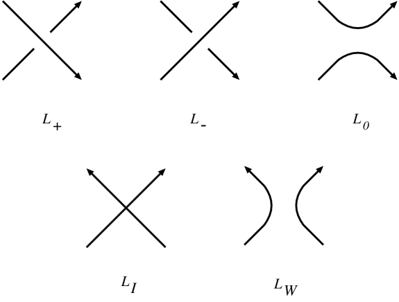
FIG. 1.: The different crossings involved in the skein relations

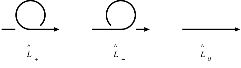
FIG. 2.: Regular isotopy invariants are not invariant under the addition and removal of a curl. This is determined by the skein relations involving the elements shown

We will show that the expression of the transform of the super Chern-Simons state satisfies related but different skein relations. In order to do this we will perform the following computation first suggested by Smolin [29] and Cotta-Ramusino et al [30]. Starting from the expression of the transform evaluated at an intersection we will append to it an infinitesimal loop in such a way as to turn the intersection into an over crossing. We will then repeat the same procedure to turn it into an under crossing. We see that the difference of the resulting expressions is related to the value of the transform evaluated at $L_{0}$ through a skein relation of the same nature of (38), but for a different polynomial.

The variation of the loop transform of the state when a small loop of element of area $\sigma^{ab}$ is appended to a single-component loop $\gamma$ at an intersection as shown in figure 3 is given by,

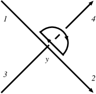
FIG. 3.: The addition of a small loop at an intersection

$$\sigma^{ab}\Delta_{ab}(y)\Psi[\gamma]=-2\Lambda i(-1)^{P}\int dA\sigma^{ab}\epsilon_{dab}{\rm STr}[{\bf G}_{I}{\bf H}_{23}(\gamma_{y}^{y}){\bf H}_{41}(\gamma_{y}^{y})]{\delta\over\delta A_{d}^{I}(y)}g^{IJ}{\rm exp}({\textstyle{i\over 2\Lambda}}S_{CS})$$ (39)

where $\Delta_{ab}$ is the loop derivative [31], $G_{I}$ is one of the generators of $GSU(2)$ and we have used $\Delta_{ab}(x){\rm STr}[{\bf H}(\gamma)]={\bf F}_{ab}^{I}(x){\rm STr}[{\bf G}_{I}{\bf H}(\gamma_{x}^{x})]$ and $\gamma_{x}^{x}$ is the loop with origin at the point $x$. The labels on the holonomy indicate the connectivity at the intersection, for instance $H_{23}$ is the loop that begins at $2$ and ends at $3$ as indicated in the figure. We have also used the fundamental property of the Chern-Simons state that we discussed in section 3,

$${\delta\over\delta{\bf A}_{a}^{I}}\Psi_{\Lambda}[A]={i\over 2\Lambda}\tilde{\epsilon}^{abc}{{\bf F}_{bc}}_{I}\Psi_{\Lambda}[A]$$ (40)

to convert the $F_{ab}$ factor due to the loop derivative into a functional derivative acting on the exponential of the Chern-Simons action. It should be recalled that indices like $I$ are raised and lowered with the orthosymplectic metric $g^{IJ}$. The factor $(-1)^{P}$ is introduced to take care of the flips in sign that take place when $F_{ab}$ is moved from the left of the supertrace to the right of it before converting it into a functional derivative and is determined by the odd/even nature of each of the components of $F_{ab}$ and the supertrace.

Integrating by parts and choosing the element of area $\sigma^{ab}$ parallel to segment 1-2 so that the contribution of the functional derivative corresponding to the action on the segment 1-2 vanishes (since the volume element is zero) we get,

$$\sigma^{ab}\Delta_{ab}\Psi[\gamma] = 2i\Lambda\int dA\sigma^{ab}\epsilon_{abc}\int dv^{c}\delta(y-v)\times$$ (42)

$${\rm STr}[{\bf G}_{I}{\bf H}_{23}(\gamma_{y}^{y}){\bf G}_{J}{\bf H}_{41}(\gamma_{y}^{y})]g^{IJ}{\rm exp}({\textstyle{i\over 2\Lambda}}S_{CS})(-1)^{JH},$$

and in the integration by parts the $(-1)^{P}$ factor is cancelled but a factor $(-1)^{JH}$ is introduced when the functional derivative is “introduced” in the supertrace at the end of the holonomy going from $2$ to $3$ and is determined by the odd/even nature of the connection in the functional derivative and the components of the holonomy going from $2$ to $3$. As is usual in these kinds of variational derivations [32], a regularization of the volume element determined by the element of area of the loop derivative and the tangent to the loop is needed, we take it in such a way that the volume is normalized to be $\pm 1$ depending on the orientation.

We now make use of the Fierz identity for $GSU(2)$,

$$g^{IJ}{({\bf G}_{I})^{\kappa}}_{\beta}{({\bf G}_{J})^{\gamma}}_{\delta} = {{\bf e}^{\kappa}}_{\delta}{{\bf e}^{\gamma}}_{\beta}-{1\over 2}{{\bf e}^{\kappa}}_{\beta}{{\bf e}^{\gamma}}_{\delta}$$ (45)

$$+{\textstyle{1\over 2}}(\delta^{\kappa}_{1}\delta^{3}_{\beta}+\delta^{\kappa}_{3}\delta^{2}_{\beta})(\delta^{\gamma}_{2}\delta^{3}_{\delta}-\delta^{\gamma}_{3}\delta^{1}_{\delta})$$

$$-{\textstyle{1\over 2}}(\delta^{\kappa}_{2}\delta^{3}_{\beta}-\delta^{\kappa}_{3}\delta^{1}_{\beta})(\delta^{\gamma}_{1}\delta^{3}_{\delta}+\delta^{\gamma}_{3}\delta^{2}_{\delta})$$

and taking into account the explicit general form of an element of $GSU(2)$ [33],

$$\left(\begin{array}[]{ccc}a(1-\alpha pq/2)&b(1-\alpha pq/2)&\sqrt{\alpha}p\\ c(1-\alpha pq/2)&d(1-\alpha pq/2)&\sqrt{\alpha}q\\ \sqrt{\alpha}(-aq+cp)&\sqrt{\alpha}(dp-bq)&(1+\alpha pq)\end{array}\right)$$ (46)

where $ad-bc=1$ and $p$ and $q$ are Grassmanian variables one finally gets,

$$\sigma^{ab}\Delta_{ab}\Psi[\gamma]=$$ (47)

$$= i\Lambda\int dA\;\sigma^{ab}\epsilon_{abc}\int dv^{c}\delta(y-v){\rm STr}[{\bf H}_{23}(\gamma_{y}^{y})]{\rm STr}[{\bf H}_{41}(\gamma_{y}^{y})]{\rm exp}({\textstyle{i\over 2\Lambda}}S_{CS})$$ (48)

$$+ i\Lambda\int dA\;\sigma^{ab}\epsilon_{abc}\int dv^{c}\delta(y-v){\rm STr}[{\bf H}_{23}(\gamma_{y}^{y}){\bf H}^{-1}_{41}(\gamma_{y}^{y})]{\rm exp}({\textstyle{i\over 2\Lambda}}S_{CS}).$$ (49)

At this point we may proceed as in the bosonic case and reinterpret relation ( 47) as a skein relation. The form of the expression we got suggests that the skein relation is,

$$\Psi[L_{\pm}]-\Psi[L_{I}]=\pm i\Lambda(\Psi[L_{0}]+\Psi[L_{W}]).$$ (50)

There is a subtle difference, however, between expression (47) and the skein relation (50). The first involves a rerouting of a portion of the loop. The implication of that rerouting for the connectivity of the loop at the intersection (the only ingredient that participates in the skein relation) is only determined given an initial connectivity of the loop at the intersection. The above skein relation corresponds to starting with a loop with a connectivity at the intersection corresponding to a single loop. One could keep the same intersection and reconnect the strands in such a way that the initial loop has two components. That requires a separate derivation for the addition of an infinitesimal element of area.

Let us therefore perform such a calculation. We consider a two component loop with an intersection as shown in figure 4,

$$\Psi(\gamma_{1},\gamma_{2})=\int dAe^{{i\over 2\Lambda}S_{CS}}W_{\gamma_{1}}[A]W_{\gamma_{2}}[A].$$ (51)

The addition of a small loop at the intersection gives, through a calculation very similar to the one performed in the case of a single component loop,

$$\sigma^{ab}\Delta_{ab}\Psi(\gamma_{1},\gamma_{2}) = 2i\Lambda\int dA\sigma^{ab}\epsilon_{abc}\int dv^{c}\delta(y-v)\times$$ (53)

$${\rm STr}[{\bf G}_{I}{\bf H}_{12}({\gamma_{1}}_{y}^{y})]\times{\rm STr}[{\bf G}_{J}{\bf H}_{43}({\gamma_{2}}_{y}^{y})]g^{IJ}{\rm exp}({\textstyle{i\over 2\Lambda}}S_{CS})(-1)^{JH_{12}},$$

and the labels refer to the figure 4.

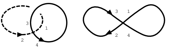
FIG. 4.: The same “straight-through” crossing can correspond to a two loop link or a single loop depending on the connectivity of the diagram.

Using the Fierz identity this expresion can be written as

$$\sigma^{ab}\Delta_{ab}\Psi(\gamma_{1},\gamma_{2})=$$ (54)

$$= i\Lambda\int dA\;\sigma^{ab}\epsilon_{abc}\int dv^{c}\delta(y-v){\rm STr}[{\bf H}_{12}({\gamma_{1}}_{y}^{y}){\bf H}_{43}({\gamma_{2}}_{y}^{y})]{\rm exp}({\textstyle{i\over 2\Lambda}}S_{CS})$$ (55)

$$- i\Lambda\int dA\;\sigma^{ab}\epsilon_{abc}\int dv^{c}\delta(y-v){\rm STr}[{\bf H}_{12}({\gamma_{1}}_{y}^{y}){\bf H}^{-1}_{43}({\gamma_{2}}_{y}^{y})]{\rm exp}({\textstyle{i\over 2\Lambda}}S_{CS}).$$ (56)

These results can be interpreted as the following skein relation for the intersection,

$$\Psi[L_{\pm}]-\Psi[L_{I}]=\pm i\Lambda(\Psi[L_{0}]-\Psi[L_{W}])$$ (57)

for the case of a two component link.

If we now replace $W(\gamma)$ by $\hat{W(\gamma)}=-W(\gamma)$ in the above expression (34,47) and in (51,54), signs change in such a way that both expressions can be associated with a single skein relation,

$$\Psi[L_{+}]-\Psi[L_{-}]=-2i\Lambda(\Psi[L_{0}]-\Psi[L_{W}]).$$ (58)

Some comments are in order. The study of the variational relation obtained by adding an infinitesimal element of area to a crossing with kinks proceeds along similar lines as the one we exhibited above. The main difference is that the volume term has two contributions that add up with opposite signs, corresponding to the addition of a small area along the two different tangents that enter the kink. With a suitable regularization, the whole contribution can be taken to be zero. This implies that an intersection with a kink can be taken as equivalent to no intersection at all, as shown in the figure 5, and this is what allow us to replace the kinks by the $L_{0}$ and $L_{W}$ in equations (47,54) to obtain the skein relations.

FIG. 5.: Intersections without (a) and with (b) kinks. Under the present regularization intersections of type (b) are equivalent to no intersection (c).

To completely characterize the polynomial, we need the value of the polynomial for the unknot, which is -1, to be consistent with the redefinition of the holonomy as minus the supertrace we introduced above. Also, since the polynomial turns out to be a regular isotopy invariant, we need to study the effect of the addition of a “curl” at a point with no intersection. The details are exactly the same as those in reference [17] so we will omit them here. The only new ingredient needed is a contraction of the Fierz identity,

$$g^{IJ}{({\bf G}_{I})^{\kappa}}_{\beta}{({\bf G}_{J})^{\beta}}_{\gamma}=\delta^{\kappa}_{\gamma},$$ (59)

and one gets as result,

$$\Psi[\hat{L}_{\pm}]=(1\pm 2\Lambda i)\Psi[\hat{L}_{0}]$$ (60)

where the meaning of the hatted elements is described in figure 2.

Let us considered now the Dubrovnik version of the Kauffman Polynomial; it is defined by the following relations [39],

$$\Psi[L_{+}]-\Psi[L_{-}] = z(\Psi[L_{0}]-\Psi[L_{W}])$$ (61)

$$\Psi[{\rm unknot}] = (a-a^{-1})/z+1$$ (62)

$$\Psi[\hat{L}_{+}] = a\Psi[L_{0}]$$ (63)

$$\Psi[\hat{L}_{-}] = a^{-1}\Psi[L_{0}]\newline$$ (64)

One can check that this correponds exactly to the results we obtained to first order provided $z=-2i\Lambda$ and $a=1+2i\Lambda$ and $\Psi[L_{0}]=-1$ which is exactly the case.

We therefore see that the Dubrovnik version of the Kauffman Polynomial bears the same relationship with a $GSU(2)$ Chern–Simons theory as the Kauffman bracket has with the usual $SU(2)$ theory. It is also important to remember that we have shown that the Dubrovnik version of the Kauffman polynomial is the transform into the loop representation of an exact quantum state of supergravity. It therefore should follow (as it happens in ordinary gravity) that the polynomial should be annihilated by all the constraints of quantum supergravity. It is also worthwhile pointing out that one could explore states without cosmological constant based on the ambient invariant polynomial associated with the one we found, as happens in the bosonic case [38].

An interesting aspect is that Saleur and Zhang [41, 42] have considered representations of the braid group associated with graded groups and found associated knot polynomials. It would be interesting to check if these have a relation with the Dubrovnik version of the Kauffman polynomial, as the calculation we have performed suggests. It would also be important to find ways to compute the skein relations we found to first order in exact form. This could be accomplished via a supersymmetric version of the Moore-Seiberg-Witten [43, 34] construction based on conformal field theory. Finally, one could evisage computing explicit expressions for each coefficient of the Dubrovnik version of the Kauffman polynomial by perturbatively evaluating the expectation value of a Wilson loop in Chern–Simons theory. For the bosonic case this was first studied by Guadagnini, Martellini, and Mintchev [44] and although more complex, the supersymmetric version of this calculation is completely feasible. This will be the first time that explicit expressions for this polynomial have been found.

V Discussion

This paper explored several issues that arise when trying to construct a loop representation for supergravity using the fact that the theory can be cast as a gauge theory of the $GSU(2)$ group. There are many detailed results that are yet to be derived, as the explicit form of the left supersymmetry constraint in the representation constructed, a complete set of Mandelstam identities and a suitable regularization for the constraint. Yet, we are already able to see the emergence of a rich mathematical structure of the representation to be constructed, in particular concerning the space of physical states of the theory. It is remarkable that a gauge theory with fermions yields a state space that only includes closed loops, contrary to what happens in other cases [36, 37]. This may be related to the extra symmetry present in supersymmetric theories equating bosons to fermions. As in the non supersymmetric case it is expected that one could find a basis of gauge invariant states that are free of Mandelstam constraints through the use of spin networks. In this case they would be spin networks associated with a graded group. The properties of such objects are yet to be explored. One could also complete the quantization of the theory in the Euclidean sector using rigorous measure theory, as has been done in the non supersymmetric case. Finally, as a by product we have showed that the knot polynomial associated with Chern-Simons theory based on a graded group is the Dubrovnik version of the Kauffman Polinomial. This is a remarkable result; it allows new insights into that polynomial and opens new perspectives in the search for the conjectured Link Polinomial [40] which has the HOMFLY and the Kauffman Polinomials as particular cases.

- [1] J. Wess, J. Bagger, “Supersymmetry and Supergravity”, Princeton Series in Physics, Princeton University Press (1983).
- [2] R. Cahn, “The eighteen arbitrary parameters of the standard model in your everyday life” preprint (1995).
- [3] See for instance A. Macias, O. Obregon and M.P. Ryan, Jr., Classical Quantum Gravity 4, 1477 (1987) and P. D’Eath, S. Hawking, O. Obregón, Phys. Lett. 300, 44 (1993).
- [4] R. Graham, C. Csordas, “Exact quantum state for supergravity”, preprint gr-qc@xxx.lanl.gov:9507008 (1995).
- [5] S. Deser, J. Kay, K. Stelle, Phys. Rev. D16, 2418 (1977).
- [6] M. Pilati, Nucl. Phys. B132, 138 (1978).
- [7] P. D’Eath, Phys. Rev. D29, 2199 (1984).
- [8] C. Teitelboim, Phys. Rev. Lett. 38, 1106 (1977).
- [9] T. Jacobson, Class. Quan. Grav. 5, 923 (1988).
- [10] A. Ashtekar (with R. Tate) , “Recent developments in nonperturbative quantum gravity”, World Scientific, Singapore (1992).
- [11] G. Fülöp, Class. Quan. Grav. 11,1 (1994).
- [12] T. Sano, J. Shiraishi, Nucl. Phys. B410, 423 (1993).
- [13] H. Matschull, Class. Quan. Grav. 11, 2395 (1994).
- [14] A. Pais, V. Rittenberg, J. Math. Phys. 16, 2062 (1975).
- [15] B. DeWitt, “Superspace, 2nd edition”, Cambridge University Press (1992).
- [16] T. Jacobson, L. Smolin, Nuc. Phys. B299, 295 (1988).
- [17] B. Brügmann, R. Gambini, J. Pullin, Nuc. Phys. B385, 587 (1992).
- [18] H. Kodama, Phys. Rev. D42, 2548 (1990).
- [19] R. Jackiw, in “Relativity, groups and topology II”, edited by B. DeWitt and L. Stora, North Holland, Amsterdam (1984).
- [20] R. Gambini, J. Pullin, Phys. Rev. D47, R5214 (1993).
- [21] R. Gambini, A. Trias, Phys. Rev. D23, 553 (1981).
- [22] C. Rovelli, L. Smolin, Nuc. Phys. B331, 80 (1990).
- [23] R. Giles, Phys. Rev. D24, 2160 (1981).
- [24] R. Gambini, A. Trias, Nucl. Phys. B278, 436 (1986).
- [25] L. Urrutia, H. Waelbroeck, F. Zertuche, Mod. Phys. Lett. A29, 2715, (1992) and references therein.
- [26] L. Urrutia, N. Morales, Lett. Math. Phys. 32, 211 (1994).
- [27] D. Berenstein, L. Urrutia, J. Math. Phys. 35, 1922 (1994).
- [28] J. Hoste, A. Ocneanu, K. Millet, P. Freyd, W. Lickorish, D. Yetter, Bull. Am. Math. Soc. 129, 239 (1985).
- [29] L. Smolin, Mod. Phys. Lett. A4 1091 (1989).
- [30] P. Cotta-Ramusino, E. Guadagnini, M. Martellini, M. Mintchev Nuc. Phys. B330, 557 (1990).
- [31] R. Gambini, J. Pullin, “Loops, knots, gauge theories and quantum gravity”, Cambridge University Press (in press).
- [32] B. Brügmann, Int. J. Theor. Phys. 34, 145 (1995).
- [33] F. Berezin, V. Tolstoy, Commun. Math. Phys. 78, 409 (1981).
- [34] E. Witten, Commun. Math. Phys 121, 351 (1989).
- [35] G. Moore, N. Seiberg, Phys. Lett. B212, 451 (1988).
- [36] R. Gambini, H. Fort, Phys. Rev. D44, 1257 (1991).
- [37] H. Morales-Técotl, C. Rovelli, Phys. Rev. Lett. 72, 3642 (1994).
- [38] B. Brügmann, R. Gambini, J. Pullin, Gen. Rel. Grav. 25, 1 (1993).
- [39] L. H. Kauffman, Knots and Physics, World Scientific, pp. 215,(1991).
- [40] L. H. Kauffman, Knots and Physics, World Scientific, pp. 54, (1991).
- [41] H. Saleur, Nucl. Phys. B336, 363 (1990).
- [42] R. Zhang, J. Math. Phys. 33, 3918 (1992).
- [43] G. Moore, N. Seiberg, Phys. Lett. B212,451 (1988).
- [44] E. Guadagnini, M. Martellini, M. Mintchev, Phys. Lett. B227, 111 (1989).