October 1994 LBL-37559

UCB-PTH-95/27

hep-th/9507155

Convergent sequences of perturbative approximations for the anharmonic oscillator
I. Harmonic approach

B. Bellet

P. Garcia

Laboratoire de Physique Mathématique
Université de Montpellier II-CNRS
34095 Montpellier cédex 05

and

A. Neveu

Theoretical Physics Group
Lawrence Berkeley Laboratory
University of California
Berkeley, California 94720

We present numerical evidence that a simple variational improvement of the ordinary perturbation theory of the quantum anharmonic oscillator can give a convergent sequence of approximations even in the extreme strong coupling limit, the purely anharmonic case. Some of the new techniques of this paper can be extended to renormalizable field theories.

Disclaimer

This document was prepared as an account of work sponsored by the United States Government. While this document is believed to contain correct information, neither the United States Government nor any agency thereof, nor The Regents of the University of California, nor any of their employees, makes any warranty, express or implied, or assumes any legal liability or responsibility for the accuracy, completeness, or usefulness of any information, apparatus, product, or process disclosed, or represents that its use would not infringe privately owned rights. Reference herein to any specific commercial products process, or service by its trade name, trademark, manufacturer, or otherwise, does not necessarily constitute or imply its endorsement, recommendation, or favoring by the United States Government or any agency thereof, or The Regents of the University of California. The views and opinions of authors expressed herein do not necessarily state or reflect those of the United States Government or any agency thereof, or The Regents of the University of California.

Lawrence Berkeley Laboratory is an equal opportunity employer.

1 Introduction.

One of us [1] has proposed a new approach to non-perturbative phenomena in quantum field theory which could combine the advantages and range of validity of ordinary perturbation theory and of variational calculations of systems with a finite number of degrees of freedom. In ref. [1], the method was applied to the first few orders of the anharmonic oscillator whose Lagrangian is:

$$L={1\over 2}\left({\partial_{t}\phi}\right)^{2}-{1\over 2}m^{2}\phi^{2}-{1\over 4}\lambda\phi^{4}$$ (1)

It gave very intriguing results: for example, the combination of a very simple variational idea with a fifth order perturbative calculation of the ground-state energy at finite $m$ gave in the purely anharmonic case $(m=0)$ a value of the ground state energy smaller than the true value by only $2.10^{-5}$, and use of the seventh order improved the relative approximation to $3.10^{-6}$; similar results were obtained for the excited states. This suggests that one could be dealing with a convergent sequence of approximations, which, if properly generalized to more complicated cases, could provide a useful computational as well as conceptual tool.

In this paper, we present a set of extensive numerical investigations on the anharmonic oscillator treated with this method. In spite of the appearance of numbers with many significant digits, we do not aim at finding exact results on the anharmonic oscillator, a very well known system. On the contrary, this paper should be read with a heuristic point of view as presenting numerical evidence in favor of a simple yet potentially powerful method to variationally improve perturbation theory in a way which remains quite empirical. To generalize the method to the more difficult case of a renormalizable field theory, one has to understand how to make it compatible with renormalization, and some of the empirical evidence gathered here turns out to be crucial for this enterprise. This will be done in other publications [2].

Some of the methods used here appear in several publications [3, 4, 5, 6], under the names “optimized perturbation theory”, “principle of minimal sensitivity”,and “delta expansion”. Here, and in our future publications [2, 10], we provide new insights and expand the range of applications of these ideas.

In section 2, exploring perturbation theory up to order $n=47$, we apply the simple variational procedure of ref. [1] to the calculation of the ground state energy in the purely anharmonic case, $m=0$, starting from the ordinary perturbative expansion at $m\neq 0$. This is equivalent to extrapolating to infinite coupling the asymptotic expansion in the dimensionless coupling constant $\lambda/\omega^{3}$, useful in principle only for weak coupling. A rather amazing picture emerges; at order $n$, the procedure yields $n$ values for the ground state energy, most of them complex with very small imaginary parts, a few of them real, all of them within a few percent (most of the time much much less) from the exact answer, $E_{0}^{exact}$. These values arrange themselves in families, increasingly numerous as the perturbative order $n$ increases, each family converging to an approximate value of $E_{0}$, the set of these approximate values itself having $E_{0}^{exact}$ as an accumulation point. We give some arguments to explain this behavior. In particular, it seems that the variational procedure generates an effective coupling constant which, as the perturbative order increases, decreases fast enough to offset the well-known factorial increase of the perturbation theory coefficients. Such an order-dependence of the effective coupling has been extensively used in refs. [4, 6], and our findings are within the range of validity of the results obtained by these authors. We show how scaling in a natural way the variational parameter with the order indeed provides much information about the large order behavior of the procedure, both for the ordinary anharmonic oscillator and on its Hartree-Fock approximation which amounts to retaining only the cactus diagrams: in large order, one obtains a remarkable improvement of the convergence of perturbation theory, the variational approximation of the ground-state energy (say) being then given by a series with an infinite radius of convergence. Furthermore, this series can be computed accurately in perturbation theory, and so the location of its extrema. Beyond its intrinsic interest, this large order result is quite important, because it turns out [2] that for renormalizable asymptotically free field theories, the variational procedure is compatible with renormalization only after the large-order limit has been taken exactly in the fashion of this section, which thus contains our main results for future use.

In section 3, we report a study of second order of perturbation theory trying to test the practical usefulness of the most general variational procedure described in ref. [1], in which the propagator is allowed an arbitrary dependence on its momentum. We have not been able to find the exact dependence which optimizes the second order of perturbation theory, but have tried ansatze with various functional forms containing a finite number of parameters. None of these more complicated forms seems to improve the approximation substantially, indicating that the simple variational ansatz of section 2, which modifies the inverse propagator by adding a constant, the result of the lowest order, captures most of the physics. This constant modification is also the Hartree-Fock approximation, or large-$N$ if one is dealing with an $O(N)$ symmetric oscillator. In section 4, we apply the method to the calculation of other physical quantities, like $<\phi^{2}>$, as a prototype of the expectation value of a composite operator, obtaining results with similar convergence properties. We also apply the method to the energy of the first excited state.

2 A Simple variational parameter.

This section, while self-contained, is an extension of some parts of ref. [1].

For the anharmonic oscillator described by the Lagrangian (1), the ordinary perturbative expansion of the ground-state energy is of the form:

$$E_{0}^{(p)}(m)={1\over 2}m+\sum_{n=1}^{p}{A_{n}\over 4^{n}}m({\lambda\over m^{3}})^{n},$$ (2)

where the coefficients $A_{n}$ can be found in ref [7]. Apart from the asymptotic behavior of $A_{n}$

$$A_{n}\sim(-3)^{n}\Gamma(n+1/2)$$ (3)

which makes the expansion (2) only Borel summable, this result at finite $p$ is useless as it stands for $m$ going to zero, the extreme strong coupling limit. However, we can introduce $\omega$ as a variational parameter, rewriting the Lagrangian (1) as:

$$L={1\over 2}\left({\partial_{t}\phi}\right)^{2}-{1\over 2}\omega^{2}\phi^{2}-{1\over 2}(m^{2}-\omega^{2})\phi^{2}-{1\over 4}\lambda\phi^{4}=L_{0}+L_{I},$$ (4)

where $L_{0}={1\over 2}\left({\partial_{t}\phi}\right)^{2}-{1\over 2}\omega^{2}\phi^{2}$ is our new free Gaussian part.

We can then compute at finite order in $L_{I}$ the ground state energy. This is done easily by starting from expansion (2), substituting

$$m=\omega\sqrt{1+(m^{2}-\omega^{2})/\omega^{2}}$$

in it, and expanding in powers of $m^{2}-\omega^{2}$ up to total order $p$ in $\lambda$ and $m^{2}-\omega^{2}$. Setting $m=0$ then gives an $\omega$-dependent approximation of order $p$ for the ground state energy of the purely anharmonic case:

$$E_{0}^{(p)}(\omega)=\sum_{n=0}^{p}{A_{n}\over 4^{n}}{\Gamma(p+n/2+1/2)\over\Gamma(3n/2+1/2)\Gamma(p-n+1)}\omega({\lambda\over\omega^{3}})^{n},$$ (5)

where $A_{0}=1/2$.

Now, if one would have started from the exact expression for the ground state energy at finite $m$, the introduction of $\omega$ should be irrelevant, and so, one may take as best approximation at finite order some value of $\omega$ such that $\partial_{\omega}E^{(p)}(\omega)=0$. This gives us a set of energy values which we can compare with the numerical value, as found in ref. [8]:

$$E_{0}^{exact}(m=0)=\lambda^{1/3}0.420804974478...\,\,.$$ (6)

Taking $\lambda=1$ , we have performed the calculation of the optima of the energy in $\omega$ until the $47^{\rm th}$ order. These results and comments on them are presented below.

2.1 Solutions of our variational problem.

The search for solutions of $\partial_{\omega}E^{(p)}(\omega)=0$ is performed in the complex plane. It gives a polynomial equation of degree $p$ in $\omega^{3}$. Most solutions of this equation are complex and give complex values for the energy, which is of course unphysical. However, quite remarkably, the imaginary part of the energy which one obtains is generally extremely small, indeed of the same order of magnitude as the error in the real part (see figure 1). Rather than simply discarding these complex extrema, one may use them as bona fide approximations, keeping only the real part and using the imaginary part as an uncertainty estimate .

If the method makes sense, of adding and subtracting an arbitrary mass term, and claiming that if one were working to all orders this should make no difference, then, at least in some range of $\omega$, $E_{0}^{(p)}(\omega)$ should be less and less dependent on $\omega$ as $p$ increases. Indeed, figures 2 and 3, where $E_{0}^{(p)}$ is plotted as a function of $\omega$ for real $\omega$ and increasing values of $p$ reveal an increasingly flat behavior around the best value, which provides a way of picking the probable best approximation when it is real and there is no imaginary part to serve as an estimate of the error.

2.2 Existence of optima families.

For a given order $p$, there are $p$ values of $\omega^{3}$ which make $E_{0}^{(p)}$ stationary. Figure 4 shows the distribution of these values for $\omega^{2}$ in the first quadrant of the complex plane, for all $p$ between 1 and 30 (the reason for choosing $\omega^{2}$ will be clear below). Obviously, they arrange themselves in families. Closer examination reveals that as $p$ is increased by 2, one “new” complex value appears in general, rather close to the real axis, which is the first member of a new family, while the other values obviously are members of families established in lower orders. The new family generally gives a better approximation than the older ones, which lie further away from the real axis. Once in a while, instead of one new complex family, two new real values appear. Figure 6 plots the values of the real optimizing values up to order 30.

2.3 Asymptotic behavior of the functions $E_{0}^{(p)}(\omega)$.

We can understand many of the features presented in the previous subsection by looking at what happens at very high order in eq. (4).

For any fixed $n$, $p$ very large, we can use Stirling’s formula, and write:

$$E_{0}^{(p)}(\omega)\sim\sum_{n=0}{A_{n}\over 4^{n}}{1\over\Gamma(3n/2+1/2)}p^{3n/2-1/2}\omega^{1-3n}.$$ (7)

where we have intentionally left the upper value of $n$ undefined. Now, from the asymptotic behavior (3) $A_{n}\sim(-3)^{n}\Gamma(n+1/2)$ we see that eq. (7) , up to an overall factor $y^{-1/3}$, defines an entire series in $y=(p/\omega^{2})^{3/2})$, and we call this function $E_{0}{(y)}$.

Many features of figures 2 and 3 can be understood in terms of this construction, which has manufactured in a new way an entire series out of an asymptotic expansion.

Let us for example explain the existence of families in figures 2 and 3. When $p$ increases, for finite values of $y$, $E_{0}^{(p)}$ as given in eq. (4) can increasingly well be approximated with $E_{0}(y)$. Hence, each extremum of $E_{0}(y)$ corresponds to a family. Furthermore, we can easily see that, in each family, $\omega^{2}/p$ and the corresponding extremum value of $E_{0}^{(p)}$ approach their asymptotic value as $1/p$. Hence, we can fit each family with an expansion in powers of $1/p$. Let us do this for the first three real families. For the first one,which starts at $6^{\rm th}$ order, we obtain:

$$E_{opt}^{(p)}\simeq 0.4207987-11.98\times 10^{-5}/p+8.991\times 10^{-5}/p^{2}+{\rm O}(p^{-3})\,.$$ (8)

For the second one, which begins at $15^{\rm th}$ order,

$$E_{opt}^{(p)}\simeq 0.420804977+5.029\times 10^{-7}/p-5.284\times 10^{-7}/p^{2}+{\rm O}(p^{-3})\,.$$ (9)

For the third one, which begins at $30^{\rm th}$ order,

$$E_{opt}^{(p)}\simeq 0.420804974472-1.25\times 10^{-9}/p-1.38\times 10^{-8}/p^{2}+{\rm O}(p^{-3})\,.$$ (10)

Including higher orders in $1/p$ does not significantly change the asymptotic values of these families.

Hence, the first real family forms a sequence of approximations which apparently converges from below to 0.4207986…, which is significantly, by about $6.10^{-6}$, less than the exact value. The second family converges from above to 0.420804977…, significantly above the exact value, by only $3.10^{-9}$. The third family converges to 0.420804974472…, still significantly below the exact value, by only about $6.10^{-12}$, which is truly remarkable. These values correspond to the successive real extrema of the function $E_{0}(y)$, which seems to display an oscillatory behavior as $y$ increases, which unfortunately seems to require going to much higher order than 47 to be seen: at that order, one sees only the first extremum. For this extremum, one finds an energy value:

$$E_{0}\simeq 0.42079845\ldots$$ (11)

Comparing this value with (8), we see that it is remarkably in agreement with the asymptotic value of the first family.

It is rather natural that no given family converge to the exact answer, as in practice this would essentially involve only a finite, if extremely large, order of the perturbative series, because of the convergence properties of the series in $E_{0}(y)$. The exact value can only be the value of $E_{0}(y)$ at $y=\infty$, as the data seems to show. So, we can try to estimate the ground state energy by an extrapolation of $E_{0}(y)$ at $y=\infty$.

2.4 Extrapolation of $E_{0}(y)$.

Instead of extrapolating $E_{0}(y)$ to $y=\infty$, we find it more convenient to perform the change of variable $X=y^{-1/3}$ and then extrapolate the function

$$E_{0}(X)=X\sum_{n=0}^{\infty}{A_{n}\over 4^{n}}{1\over\Gamma(3n/2+1/2)}X^{-3n}$$ (12)

to $X=0$, knowing that:

i) $E_{0}(X)$ behaves asymptotically as $X$ for $X\rightarrow\infty$,

ii) for $X<<1$, this function has a sequence of very flat extrema, and goes exponentially fast to the exact value $E_{0}^{exact}$ as $X\rightarrow\infty$, which is the number we are looking for.

For this extrapolation, it seems easiest to consider the derivative of $E_{0}(X)$, which satisfies

$$\lim_{X\rightarrow\infty}\partial_{X}E_{0}(X)={1\over{2\sqrt{\pi}}}\,,$$ (13)

impose a decreasing exponential behavior at $X=0$, and find the value of $E_{0}(X=0)$ by integration from infinity to zero. For example, we can fit this function, $\partial_{X}E_{0}(X)$, at $X\rightarrow\infty$, using the functional form

$$\partial_{X}E_{0}(X)={1\over{2\sqrt{\pi}}}\exp(-a/X^{3})[1+b/X^{3}+c/X^{6}+\ldots].$$ (14)

with appropriate values of the parameters $a,b,c\ldots$

This extrapolation procedure can be considered as an alternative to the extremization procedure of the previous subsections, using the same numerical information, encoded in the values of the successive perturbation theory coefficients $A_{0},A_{1},A_{2}\ldots$ We thus obtain:

- Using only $A_{0}$ and $A_{1}$, $i.e.$ setting $b=c=\ldots=0$:

$$E_{0}^{appr}=0.420014\ldots$$ (15)

which must be compared with the usual variational value $E_{0}^{(1)}=0.429268\ldots$ and the exact $E_{0}^{exact}\simeq 0.420805$. Remarkably, taking into account only the first order Feynman diagram, we thus obtain an approximate value below the exact ground state energy by only $8\times 10^{-3}$! This is actually due to the fact that in the next approximations, the coefficient $b$ is accidentally very small. An accuracy of a few percent would probably be more generic.

- Using $A_{0}$, $A_{1}$ and $A_{3}$,

$$E_{0}^{appr}=0.4204619\ldots$$ (16)

to be compared with $E_{0}^{(2)}=0.421218\ldots+0.0014\ldots{\rm i}$,

- Using $A_{0}$, $A_{1}$, $A_{3}$ and $A_{4}$,

$$E_{0}^{appr}=0.420474\ldots$$ (17)

to be compared with $E_{0}^{(3)}=0.420983\ldots$

We see that this extrapolation method of the entire function $E_{0}(y)$ gives remarkably good numerical values, and has the further advantage of giving real numbers. The functions analogous to $E_{0}(y)$ will play a crucial rôle in the quantum field theory case, as it turns out to be the main feature of this paper which survives renormalization and its infinities.

2.5 Oscillatory behavior of $E_{0}(X)$ in the case of the Hartree-Fock approximation.

In this subsection, we report the results of the procedures of the previous subsections applied to the theory restricted to the Hartree-Fock approximation (if we were dealing with an $N$-component symmetric oscillator, this would correspond to taking the large-$N$ limit). The advantage of the Hartree-Fock case is that ordinary perturbation theory of the Lagrangian (1) has a finite radius of convergence in $\lambda/m^{3}$. We shall see that the features discovered in the previous subsections are naturally also present in this approximation, together with a couple of extra ones.

The Hartree-Fock approximation of the ground-state energy is given by the sum of all vacuum to vacuum cactus Feynman diagrams. Applying the same procedure as in section 1, we obtain for the order-$p$ approximation at $\lambda=1$:

$$E_{H.F.}^{(p)}(\omega)=\sum_{n=0}^{p}{C_{n}\over 4^{n}}{\Gamma(p+n/2+1/2)\over\Gamma(3n/2+1/2)\Gamma(p-n+1)}\omega({1\over\omega^{3}})^{n}\,,$$ (18)

where the coefficients $C_{n}$ give the sum of all cactus graphs of order $n$. This is the expression, identical in form to equation (5), which has to be studied in our variational approximation.

In the framework of this approximation, we obtain many real solutions of the variational equation (see figure 5) to be compared with the exact value

$$E_{H.F.}^{exact}=0.4292678409575\ldots$$ (19)

Remarkably, at any order, the exact value is one of the solutions of the variational procedure, the one corresponding to the smallest value of $\omega$, which sits precisely at the edge of the convergence region of the original perturbative series. This coincidence is of course a pathology unique to the Hartree-Fock approximation, which corresponds to the fact that in the full theory, the variational value for the energy which gives the best numerical value is the one for the smallest $\omega$. Apart from that, the grouping of the values of $\omega$ in families, and the oscillatory behavior of the function $E_{H.F.}^{(p)}(\omega)$ are much the same as in the full theory.

Next, as in subsection (2.3), we go to the limit $p\rightarrow\infty$ with the same rescaling of $\omega$, and define the function:

$$E_{H.F.}(y)=y^{-1/3}(\sum_{n=0}^{\infty}{C_{n}\over 4^{n}}{1\over\Gamma(3n/2+1/2)}y^{n}).$$ (20)

Because the $C_{n}$ coefficients are those of a series with finite radius of convergence, one can obtain much better estimates of the series in this equation for large values of $y$, and thus see very well its oscillating behavior in that region, which was not the case for the full theory. This is displayed in figures 7 and 8.

We can for example compare several asymptotic energy values associated with the families displayed in fig. 5 with the stationary values of $E_{H.F.}(y)$. For the first three families,we find:

- First family:

$$E_{opt}^{(p)}=0.428584-0.00382794/p+0.00244357/p^{2}+{\rm O}(p^{-3}),$$ (21)

and for the corresponding extremum of $E_{H.F.}(y)$:

$$E_{H.F.}^{ext}=0.42857\ldots$$ (22)

- Second family:

$$E_{opt}^{(p)}=0.4292937645-0.00051/p+0.00031/p^{2}+{\rm O}(p^{-3}),$$ (23)

and

$$E_{H.F.}^{ext}=0.429297\ldots$$ (24)

- Third family:

$$E_{opt}^{(p)}=0.4292674287-0.000096/p-0.00021/p^{2}+{\rm O}(p^{-3}),$$ (25)

and

$$E_{H.F.}^{ext}=0.4292659\ldots$$ (26)

By applying our variational procedure to the Hartree-Fock approximation and comparing with the full theory, we thus see which features are more generic, and hence have a better chance of surviving in field theory. We think that the main lesson to be learned is that the exact Hartree-Fock result, already found at lowest order, and common in that order to the Hartree-Fock case and to the complete theory may be misleading, in the sense that it seems to give too much weight to the fact that the variational method gives the exact result for the Hartree-Fock case. In contrast to this possibly pathological coincidence, the behavior of the large-order limit function $E_{0}(X)$ is common to the Hartree-Fock case and to the complete theory. This large-order limit also sheds light on the general behavior of the curves of figures 2 and 3 : the regular shift to the right of the right-hand parts of the curves exactly corresponds to the rescaling of $\omega^{2}$ by the order in the large-order limit. For the left-hand parts of the curves, they do not shift to the right in the case of the Hartree-Fock approximation, and shift to the right in the complete theory only as $\omega^{3}$ proportionnal to the order. Thus, in both cases, there is an increasing region in $\omega$ where the curves become flatter as the order increases and hence, the approximation more and more accurate. These scaling behaviors correspond to those found in reference [6]. Furthermore, the limiting function $E_{0}(X)$ can be computed in perturbation theory for large $X$, and, as we have seen in subsection (2.4), accurately extrapolated to $X=0$ to give an excellent value of the energy, and we shall see in our extension to quantum field theory [2] that this is indeed the most robust feature of this section, robust enough to survive renormalization.

3 More sophisticated approach: the use of several parameters.

In the previous section, our variational improvement of perturbation theory has been severely restricted to the class of variational ansatze where the modification of the inverse propagator is a constant. It would be worthwhile to have an idea of the improvement which a more general modification would give.

The variational improvement of perturbation theory provides an order-dependent equation for the modified propagator $G=1/(k^{2}-K)$ which at first and second orders is depicted by the Feynman diagrams of figures 9 and 10, in which the internal lines involve the modified propagator $G$ itself.

In principle, the most arbitrary $G$ could involve a complicated kernel, but it is obvious that there should exist solutions of these equations of the form $G(k)=1/[k^{2}-K(k)]$ (more general kernels $G(k,k^{\prime})$ would occur naturally if one were looking for solutions corresponding to bound states, and must exist, as indeed the functional equation of figure 9 is identical to equation (2.14) of reference [11] which has a very rich set of solutions. However, pursuing investigations in that direction would go beyond the scope of the present paper). In lowest order, a solution of this form will automatically lead to a constant $K$, solution of the Hartree-Fock approximation. In second order, because of the non-trivial structure of the last diagram in Fig. 10, $K(k)$ must be non constant. The equation which $K$ satisfies is an unusual non-linear integral equation for which we have found no clever trick. Hence, we resort once more to a further approximation, in which we restrict $K(k)$ to certain functional forms with a finite number of variational parameters in them with respect to which we optimize. We now list these various functional forms in Euclidean notation and the corresponding results of the optimization.

For reference, we first give the values for the simple ansatz of the previous section:

i)For $G(k)=1/(k^{2}+m^{2})$ :

$$m\simeq 1.2980+0.0083\,{\rm i}$$ (27)

which gives:

$$E_{opt}\simeq 0.42142+0,00013\,{\rm i}$$ (28)

Moving to increasingly complicated ansatze, we have:

ii)For $G(k)=\alpha/(k^{2}+m^{2})$ :

$$\alpha \simeq 0.9836+0.1511\,{\rm i}$$ (29)

$$m \simeq 1.3102+0.0427\,{\rm i}$$

which give:

$$E_{opt}\simeq 0.42169+0.00014\,{\rm i}\,.$$ (30)

and

$$\alpha \simeq 0.9423+0.087\,{\rm i}$$ (31)

$$m \simeq 1.1957+0.1915\,{\rm i}$$

which give:

$$E_{opt}\simeq 0.42049+0.00152\,{\rm i}\,.$$ (32)

iii)For $G(k)=\alpha/(k^{2}+m^{2})+(1-\alpha)/(k^{2}+n^{2})$ :

$$\alpha \simeq 0.8979-0.0442\,{\rm i}$$

$$m \simeq 1.1833+0.0655\,{\rm i}$$ (33)

$$n \simeq 7.6246-2.0266\,{\rm i}$$

which give:

$$E_{opt}\simeq 0.42096+0.00099\,{\rm i}\,.$$ (34)

iv)For $G(k)=\alpha/(k^{2}+m^{2})+\beta/(k^{2}+n^{2})+(1-\alpha-\beta)/(k^{2}+u^{2})$ :

$$\alpha \simeq 0.9105+0.0678\,{\rm i}$$

$$\beta \simeq 0.0989-0.0233\,{\rm i}$$

$$m \simeq 1.1902-0.0458\,{\rm i}$$ (35)

$$n \simeq 3.1798+5.1317\,{\rm i}$$

$$u \simeq 5.1534+18.30\,{\rm i}$$

which give:

$$E_{opt}\simeq 0.42095-0.00098\,{\rm i}\,.$$ (36)

iv)For $G(k)=1/(k^{2}+\alpha|k|+m^{2})$ :

$$\alpha \simeq 0.1751-0.1459\,{\rm i}$$ (37)

$$m \simeq 1.2222+0.1509\,{\rm i}$$

which give:

$$E_{opt}\simeq 0.42084+0.00129\,{\rm i}\,.$$ (38)

and

$$\alpha \simeq 0.0198+0.2957\,{\rm i}$$ (39)

$$m \simeq 1.2844+0.0459\,{\rm i}$$

which give:

$$E_{opt}\simeq 0.42149+0.00090\,{\rm i}\,.$$ (40)

We should note that these results are not as exhaustive as in the previous section, because we must look for the extrema in the complex planes of several parameters, where it is easy to get lost: there may be other extrema, in some far away regions of parameter space. Nevertheless, we believe that the following qualitative picture emerges: Such optimizations do not seem to increase appreciably the accuracy on the ground state energy whether measured by the value of the imaginary part of $E_{opt}$ or by the difference of the real part with the true value: this accuracy remains around $10^{-3}$. We may reasonably conjecture that this is indeed as well as the method can do at this second order, and that solving the variational equation exactly for the propagator at that order would not give any substantial improvement beyond the result of the simple ansatz of the previous section.

4 Calculation of other physical quantities.

4.1 Mean value of $<\phi^{2}>$:

Vacuum expectation values of composite operators are objects of great physical interest in quantum field theories, much more than in ordinary quantum mechanics. For example, they play an important rôle in chiral perturbation theory, and it would be most welcome to have even rather crude approximations for their values. Hence, in this section, we shall investigate the accuracy with which our method can give $<\phi^{2}>$ in the ground state of the anharmonic oscillator.

We shall also use this calculation to test another idea: although it is clear that, as in any variational procedure, one would in principle get the best results by optimizing the quantity of interest with respect to the variational parameters, it is sometimes tempting to use the values of the parameters obtained in the optimization of some quantity (in the present case the ground state energy) in order to compute other quantities with them, particularly if these other quantities give rise to some unwieldy set of variational equations (this could occur for example for a propagator or some more complicated correlation function which have some space-time variables in them). We are thus going to compare the results of these two procedures for the ground state expectation value $<\phi^{2}>$. From

$$E_{0}(m,\lambda)=<-{1\over 2}{d^{2}\over d\phi^{2}}+{1\over 2}m^{2}\phi^{2}+\frac{\lambda}{4}\phi^{4}>,$$ (41)

we have simply

$$<\phi^{2}>=2\frac{\partial}{\partial m^{2}}E_{0}(m,\lambda)$$ (42)

so that the perturbative expansion at non-zero $m$ of $<\phi^{2}>$ is rather trivially obtained from equation (2), and one can then proceed as in section (2): At $m=0$, we have thus computed the optima with respect to $\omega$ up to order 30, and compared them with the value found in ref. [9]:

$$<\phi^{2}>_{exact}=\lambda^{-1/3}\,\,0.456119955748\ldots$$ (43)

We have found convergence and accuracy properties very similar to those of the ground-state energy itself as described in section (2), and we do not report here the details.

Next, we compare the results of optimizing directly $<\phi^{2}>$ with the value obtained by using the $\omega$ obtained from the optimization of the ground-state energy in the same order. For the direct calculation to orders $p=1$ to 3, we obtain:

$${\rm for}\,\,\,p=1:\,\, \omega\simeq 1.25992 <\phi^{2}>\simeq 0.44645$$

$${\rm for}\,\,\,p=2:\,\, \,\omega\simeq 1.34807+0.11106\,{\rm i}\, \,<\phi^{2}>\simeq 0.45575-0.00227\,{\rm i}$$

$${\rm for}\,\,\,p=3:\,\, \omega\simeq 1.43806 <\phi^{2}>\simeq 0.45592$$

$$\omega\simeq 1.40288+0.17821\,{\rm i}\, \,<\phi^{2}>=0.45723-2.7\times 10^{-5}{\rm i}$$

while using the values of $\omega$ obtained from the optimization of the ground-state energy at the same order, we obtain

$${\rm for}\,\,\,p=1:\,\, \omega\simeq 1.14471 <\phi^{2}>\simeq 0.43678$$

$${\rm for}\,\,\,p=2:\,\, \,\omega\simeq 1.27264+0.12645\,{\rm i}\, \,<\phi^{2}>\simeq 0.45424-0.00389\,{\rm i}\,$$

$${\rm for}\,\,\,p=3:\,\, \omega\simeq 1.37080 <\phi^{2}>\simeq 0.45549$$

$$\omega\simeq 1.35091+0.19488\,{\rm i}\, \,<\phi^{2}>\simeq 0.45744-6.8\times 10^{-4}{\rm i}$$

Comparing these numbers with the exact value (43), we see that these two approaches lead to results with the same order of accuracy, the direct optimization doing only slightly better. In the next subsection, we shall perform a similar comparison for another quantity.

4.2 Energy of the first excited state

We can use the perturbative expansion for the energy of the first excited state,

$$E_{1}(m,\lambda)=\frac{3}{2}m+\frac{15}{16}\frac{\lambda}{m^{2}}-\frac{165}{128}\frac{\lambda^{2}}{m^{5}}+\frac{3915}{1024}\frac{\lambda^{3}}{m^{8}}$$ (46)

and repeat on it the optimization of section (2) up to order 3. We obtain a sequence of approximations with very similar features. The results for the first three orders $p$ are:

$${\rm for}\,\,\,p=1:\,\, \omega\simeq 1.35721 E_{1}^{(1)}\simeq 1.52686$$ (47)

$${\rm for}\,\,\,p=2:\,\, \,\omega\simeq 1.49893+0.08752\,{\rm i}\, \,E_{1}^{(2)}\simeq 1.50739+0.001\,{\rm i}$$

$${\rm for}\,\,\,p=3:\,\, \omega=1.69418 E_{1}^{(3)}\simeq 1.50710$$

$$\omega\simeq 1.53709-0.11684\,{\rm i}\, \,E_{1}^{(3)}\simeq 1.50750+5.8\times 10^{-4}{\rm i}$$

which can be compared to the accurate value:

$$E_{1}^{exact}=1.50790125\ldots$$ (48)

One may now compare these results with those obtained by evaluating $E_{1}^{p}$ at the optima of $E_{0}^{p}$ for the same value of $p$. This gives:

$${\rm for}\,\,\,p=1:\,\, \omega\simeq 1.14471 E_{1}^{(1)}\simeq 1.57398$$ (49)

$${\rm for}\,\,\,p=2:\,\, \,\omega\simeq 1.29802+0.00828\,{\rm i}\, \,E_{1}^{(2)}\simeq 1.49323+0.0016\,{\rm i}$$

$${\rm for}\,\,\,p=3:\,\, \omega\simeq 1.37080 E_{1}^{(3)}\simeq 1.51382$$

$$\omega\simeq 1.35091-0.19449\,{\rm i}\, \,E_{1}^{(3)}\simeq 1.49385+0.00075\,{\rm i}$$

Although the true optima of $E_{1}^{(p)}$ are indeed much closer to the exact answer than the values at the optima of $E_{0}^{(p)}$, these nevertheless provide quite reasonable approximations, which improve when the order increases, due to the increasingly flat character of the corresponding function, analogous to what can be seen on figures 2 and 3.

Another way to compute the energy of the first excited state is to use the 2-point 1-P-I function at order $p$, $\Gamma^{(p)}(k)$ which vanishes for $k=E_{1}-E_{0}$. Figure 11 shows the Feynman diagrams to be computed up to second order of perturbation theory.

In general, a direct optimization of this function would have to be made for each value of $k$. In first order, taking $1/(k^{2}+\omega^{2})$ as variational ansatz, one obtains

$$\Gamma_{(2)}(k,\omega)=k^{2}+\frac{3}{2}\frac{\lambda}{\omega},$$ (50)

which has no extremum in $\omega$: the only natural thing to do at that order is thus to plug in the value of $\omega$ obtained in the optimization of the ground-state energy: this gives back the Hartee-Fock value for the mass gap, $1.1447142\ldots$ (at $\lambda=1$), while the correct value is $E_{1}^{exact}-E_{0}^{exact}=1.087096\ldots$

In second order, taking again simply $1/(k^{2}+\omega^{2})$ as variational ansatz, one obtains:

$$\Gamma_{(2)}(k,\omega)=k^{2}-\frac{9}{4\omega}+\frac{9\lambda}{2\omega}\bigl{(}\frac{1}{4\omega^{2}}+\frac{1}{k^{2}+9\omega^{2}}\bigr{)}.$$ (51)

Hence, one can solve the sytem

$$\partial_{\omega}\Gamma_{(p)}(k,\omega)=0,$$ (52)

$$\Gamma_{(p)}(k,\omega)=0,$$ (53)

obtaining at $\lambda=1$:

$$\omega\simeq 1.4107698$$ (54)

$$k=E_{1}-E_{0}\simeq 1.092026$$ (55)

which is about $10^{-3}$ away from the correct value, i.e. an error of the same order of magnitude as in the calculations of $E_{0}$ or $E_{1}$ at the same order, except that it has the advantage of being real (by chance, as far as we can tell). By contrast, plugging in $\Gamma_{(p)}(k,\omega)$ the (complex) value of $\omega$ obtained from the optimization of $E_{0}^{(2)}$ and looking for the zero gives an error of a few percents in $E_{1}-E_{0}$, compared to the $\simeq 10^{-3}$ error seen in equation (55). Using the more complicated anstze of the end of section 3 give similar results, and we do not report them here.

In this section, we have seen that the procedure of [1] can be used successfully to compute a variety of physical quantities. In each case, as expected from a variational approximation, directly optimizing the quantity of interest gives the best answer, but using the values of the variational parameters from the optimization of another quantity is not necessarily bad: the loss of numerical accuracy seems of the same order as working in one order less in perturbation theory.

5 Conclusion

In this first paper, we have first explored in numerical detail the remarkable convergence properties of the variational method proposed in [1] on the particular case of the ground-state energy of the anharmonic oscillator. We have found how the extrema arrange themselves in families, and how these families converge to the exact answer. We have seen that these families are also present in the Hartree-Fock approximation, and in the calculation of other physical quantities.

Although higher orders of the variational procedure do not give bounds (contrary to the usual lowest order), this is compensated by its straighforward applicability to the calculation of excited states or expectation values.

Going to infinite order in the (easy) variational procedure (which involves only a modification of the free Lagrangian) but finite order in the (hard) perturbative calculation (which involves the quartic interaction term), we have put some order in these families, improved the convergence of the perturbative series by a factorial, and defined an extrapolation procedure which is not only numerically excellent, but will be seen in future publications [2] to generalize to the case of renormalizable field theory.

In the next paper [10], we shall see how a similar variational improvement of perturbation theory can be achieved through a variational ansatz corresponding to putting the anharmonic oscillator in a finite time box.

6 Acknowlegments

One of us (A. N.) is grateful for their hospitality to the Lawrence Berkeley Laboratory, where this work was supported in part by the Director, Office of Energy research, Office of High Energy and Nuclear Physics, Division of High Energy Physics of the U.S. Department of Energy under Contract DE-AC03-76SF00098 and to the Physics Department, University of California, Berkeley, where this work was completed with partial support from National Science Foundation grant PHY-90-21139.

Figure 1: In a base-10 log-log diagram, the imaginary part of the energies versus the error on their real part.

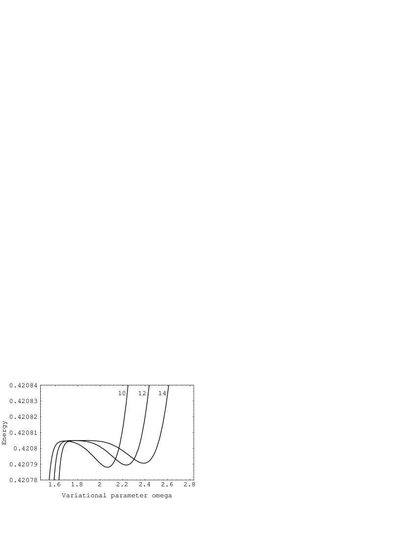
Figure 2: $E_{0}(\omega)$ for orders 10, 12 and 14.

Figure 3: $E_{0}(\omega)$ for orders 11, 13 and 15.

Figure 4: Distribution of the $\omega_{opt}^{2}$ in the first quadrant of the complex plane.

Figure 5: The real $\omega_{opt}^{2}$ versus the perturbation order in the Hartree-Fock approximation.

Figure 6: The real $\omega_{opt}^{2}$ versus the perturbation order.

Figure 7: $E_{H.F.}(X)$ where $X=y^{-1/3}$, plotted using the 50 first terms of the series (20).

Figure 8: Zooms of figure 7.

Figure 9: First order “gap equation”.

Figure 10: Second order “gap equation”.

Figure 11: 1-P-I diagrams of $\Gamma^{(2)}(k)$.

References

- [1] A.Neveu, Nucl. Phys. B 18 (1990) 242.
-
[2]
C. Arvanitis, F. Geniet and A. Neveu,
“Variational solution of the Gross-Neveu model,
I. The large- limit”, Montpellier preprint PM94-19
(hep-th/9506188);
C. Arvanitis, F. Geniet, J.-L. Kneur, M. Iacomi and A. Neveu, “Variational solution of the Gross-Neveu model, II. Finite- and renormalization”, Montpellier preprint PM94-20, to be published. -
[3]
W.E. Caswell, Ann. Phys. (N.Y) 123 (1979) 153;
I.G. Halliday and P. Suranyi, Phys. Lett. 85 B (1979) 421;
P.M. Stevenson, Phys. Rev. D 23 (1981) 2916;
I. Stancu and P.M. Stevenson, Phys. Rev. D 42 (1990) 2710;
J. Killinbeck, J. Phys. A 14 (1981) 1005. - [4] R. Seznec and J. Zinn-Justin, J. Math. Phys. 20 (1979) 1398.
-
[5]
A. Okopinska, Phys. Rev. D 35 (1987) 1835;
A. Duncan and M. Moshe, Phys. Lett. 215 B (1988) 352;
H.F. Jones and M. Moshe, Phys. Lett. 234 B (1990) 492;
S. Gandhi, H.F. Jones and M. Pinto, Nucl. Phys. B 359 (1991) 429;
S. Gandhi, M. Pinto, Phys. Rev. D 46 (1992) 2570;
A.N. Sissakian, I.L. Solovtsov and O.P. Solovtsova Phys. Lett. 321 B (1994) 381;
A. Duncan and H.F. Jones, Phys. Rev. D 47 (1993) 2560;
C.M. Bender, A. Duncan and H.F. Jones, Phys. Rev. D 49 (1994) 4219;
C. Arvanitis, H.F. Jones and C. Parker, Imperial College preprint TP/94-95/20 (hep-ph/9502386) to be published. - [6] R. Guida, K. Konishi and H. Suzuki, Genova Preprints GEF-Th-7/1994 (hep-th/9407027) and GEF-Th-4/1995 (hep-th/9505084).
- [7] C.M. Bender and T.T. Wu, Phys. Rev. 184 (1969) 1231.
- [8] C.M. Bender, K. Olaussen and P.S. Wang, Phys. Rev. D 16 (1977) 1780.
- [9] K. Banerjee, S.P. Bhatnagar, V. Choudhry and S.S. Kanwal, Proc. R. Soc. Lond. A 360 (1978) 575-586.
- [10] B. Bellet, P. Garcia and A. Neveu, “Convergent sequences of perturbative approximations for the anharmonic oscillator, II. Compact time approach”, Montpellier preprint, next paper.
- [11] R.F. Dashen, B. Hasslacher and A. Neveu, Phys. Rev. D 12 (1975) 2443.