Source Galerkin Calculations in
Scalar Field Theory

In this paper, we extend previous work on scalar $\phi^{4}$ theory using the Source Galerkin method. This approach is based on finding solutions $Z[J]$ to the lattice functional equations for field theories in the presence of an external source $J$. Using polynomial expansions for the generating functional $Z$, we calculate propagators and mass-gaps for a number of systems. These calculations are straightforward to perform and are executed rapidly compared to Monte Carlo. The bulk of the computation involves a single matrix inversion. The use of polynomial expansions illustrates in a clear and simple way the ideas of the Source Galerkin method. But at the same time, this choice has serious limitations. Even after exploiting symmetries, the size of calculations become prohibitive except for small systems. The calculations in this paper were made on a workstation of modest power using a fourth order polynomial expansion for lattices of size $8^{2}$,$4^{3}$,$2^{4}$ in $2D$, $3D$, and $4D$. In addition, we present an alternative to the Galerkin procedure that results in sparse matrices to invert.

bla BROWN-HET-966

1 Introduction

Previously, we presented a new numerical approach to quantum field theory called the Source Galerkin method [1]. This deterministic approach is fundamentally different from other attempts to solve lattice theories. It is based on finding solutions to the lattice functional equations for field theories in the presence of an external source. The object of calculations is a generating function $Z$ which is a multivariate function of the discretized sources $J_{i}$. There is one source variable for each site of the lattice. Once an approximate solution for $Z$ is found, the Green’s functions can be extracted by differentiation. This formulation is identical for fermions, the only difference being that the fermionic sources anticommute [3].

Despite the large number of coupled differential equations for $Z$, one for each source variable, there is nothing unusual about this problem mathematically. For scalar $\phi^{4}$, the functional relations are a set of third order linear differential equations. We can solve them as we do any set of linear differential equations. Since at the end of any calculation the sources are set to zero, the obvious first choice is to expand $Z$ in a power series in the sources about the origin. Since we cannot solve the theory exactly, we must introduce an approximation. For the purposes of this paper, we truncate the series expansion for $Z$ after some maximum power in the source variables. In this way, we obtain a closed, finite set of linear equations for the expansion coefficients accurate to within the limits of the approximation.

This approach has many advantages because of the simple structure of Taylor series expansions. However, the computational complexity of this particular expansion scheme increases rapidly with system size. As a result, truncated series can only be used for small systems. Nevertheless, due to the accuracy of this method, it is possible to extract large amounts of information about the system with only short computer runs. It should be emphasized that this shortcoming does not represent an intrinsic limit of the Source Galerkin method, but rather is a reflection of choosing power series basis functions. Using this basis we are able to display many of the features that make the Galerkin method so powerful for controlling the error resulting from approximations. Because Taylor expansions are so simple, we are able to present another interesting method to deal with truncated series expansions. Elsewere, we develop more appropriate expansion functions and more general numerical procedures. These are necessary for Galerkin based examinations of larger systems.

The next sections are organized as follows. In Section I, we give a review of the Source Galerkin method. In Section II, we work out a simple example for a two site model to illustrate the method and expose its structure. Next, we find symmetry to be a valuable tool for reducing the size of calculations. By constructing the power series to reflect explicitly the lattice symmetries, we significantly reduce the number of unknowns in our problem. In Section III, we give a systematic method to construct lattice invariant polynomials. These polynomials will form a basis for our solutions. In Section IV, we present results for numerical calculations on systems for scalar $\phi^{4}$ theory in $D=2,3,4$. Comparisons with Monte Carlo simulations are shown. Finally, in Sections V,VI, we present an alternative to the Galerkin method applied to Taylor series test functions. Using this method we introduce a flatness criterion to control the convergence of approximations. This approach does not solve the problem of increasing computational complexity, but does result in sparse matrices to invert at the end of calculations.

2 Source Galerkin Method

We study quantum field theory in the presence of an external source. The vacuum persistence amplitude $Z[J]=_{J}\langle 0|0\rangle_{J}$ is the generating functional for the Green’s functions. It is constrained by a functional differential equation. For a self-interacting scalar field theory, the dynamics are described by

$$L_{J}\,(\phi)\;=\;1/2\,\hat{\phi}\;(\Box+M^{2})\;\hat{\phi}\;+\;g/4\,\hat{\phi^{4}}\;+\;J\hat{\phi}.$$ (1)

Taking vacuum expectation values of the operator equations of motion

$$(\Box+M^{2})\langle\hat{\phi}\rangle_{J}\;+\;g\,\langle\hat{\phi^{3}}\rangle_{J}\;=\;J\,_{J}\langle 0|0\rangle_{J}$$ (2)

and identifying Euclidean space expectation values of fields with functional derivatives of $Z[J]$

$$G(x_{1}\ldots x_{n})\;=\;\frac{\delta^{n}Z[J]}{\delta J(x_{1})\ldots\delta J(x_{n})}$$ (3)

yields the functional relation

$$(\Box+M^{2})\,\frac{\delta Z}{\delta J(x)}\;+\;g\,\frac{\delta^{3}Z}{\delta J(x)^{3}}\;=\;J\;Z.$$ (4)

After solving this equation for $Z$, we can extract all information about our field theory by functional differentiation. On a $D$-dimensional Euclidean lattice, the functional equation becomes a set of coupled differential equations

$$(2\,D+M^{2}){\partial Z\over\partial{J(i)}}-\sum_{nn}{\partial Z\over\partial{J(i)}}+g{{\partial^{3}Z}\over{\partial{J(i)^{3}}}}=J(i)Z$$ (5)

where the sum is over nearest neighbors. There is one equation per site.

For finite lattices with $N$ sites, we construct $Z$ as a multivariate function of the $N$ source variables $J(i)$. To construct a solution to the differential equations, we can expand $Z$ on any complete set of functions in the source variables

$$Z\hskip 7.22743pt=\hskip 7.22743pt\sum_{n}\;a_{n}\,\phi_{n}(\{J\})$$ (6)

where the $a_{n}$ are the unknowns of the problem. A particularly simple choice is polynomial functions. It should be emphasized that other choices are possible, and indeed preferred, for more complicated systems. In this paper, we consider only polynomial expansions.

The number of independent unknown coefficients in our expansion can be reduced by exploiting the symmetries of the lattice. $Z$ is constructed to be invariant under the symmetry group of the lattice

$$Z\hskip 7.22743pt=\hskip 7.22743pt\sum_{n,m}\;a_{n,m}\,P_{n,m}$$ (7)

where $P_{n,m}$ are invariant polynomials in the source variables of order $n$ and with $m$ invariant classes for a given order. The coefficients $a_{n,m}$ are to be determined. The number of invariant classes for a given order depends on both the number of lattice sites and on the number of symmetry operations for a given lattice. For example, higher dimensional lattices have larger symmetry groups, and therefore have fewer independent unknowns. They form a lattice invariant basis upon which we construct solutions for $Z$.

In order to solve the differential equations, we must specify boundary conditions. We normalize the vacuum amplitude

$$Z[J=0]=1$$ (8)

and we require odd Green’s functions vanish

$$\frac{dZ}{dJ(i)}|_{J=0}=\langle\phi(i)\rangle=0.$$ (9)

Rather than specify the second derivatives of $Z$, the two-point functions, we set the third boundary condition by truncating $Z$ at some finite order. The truncation order is dictated by computational constraints. As a boundary condition, truncation guarantees that as $g\rightarrow 0$ in the interacting theory, the solution reduces to the free field. This is possible only for path integral formulations constrained to real integration contours [2, 4, 5]. Truncation in this sense not only sets a boundary condition, but also introduces an approximation scheme. This scheme is made systematic by truncating at successively higher orders.

In order to fit our truncated solution $Z_{T}$ to a solution of the differential equations, we use the Galerkin method [6]. This is a spectral method well-known in applied mathematics, and is especially well-suited to our problem. In this approach, given a differential equation

$$\hat{D}\,Z[\,J\,]=0,$$ (10)

we can define a residual function $R$

$$R=\hat{D}_{i}\,Z_{T}$$ (11)

where $\hat{D}_{i}$ is the differential source operator centered at site $i$. If $Z_{T}$ were the exact solution, then $R$ would be identically zero. But since $Z_{T}$ is approximate, it is necessarily a nontrivial function of the source variables. The residual is a direct measure of the error due to approximation. We will fit our solution by minimizing $R$. To implement this, we define an inner product in the source space

$$(g,f)=\int_{-\epsilon}^{\epsilon}g(J(1)\ldots J(N))f(J(1)\ldots J(N))\,[dJ]$$ (12)

where the integration is over all $J(i)$, and $\epsilon$ is considered small. Requiring the inner product

of $R$ with linearly independent test functions $T_{k}$ to vanish

$$(R,T_{1}) = 0$$

$$\vdots$$ (13)

$$(R,T_{j}) = 0$$

generates a set of linear algebraic equations. We can generate as many of these equations as we like as long as the $T_{k}$ are linearly independent.

In analogy with a variational principle, we chose the test functions as

$$T_{k}\hskip 7.22743pt=\hskip 7.22743pt\frac{d}{dJ(1)}\;P_{n,m}$$ (14)

where the $P_{n,m}$ are the invariant polynomial that formed the basis for $Z_{T}$ . This choice guarantees that we always have as many equations as unknowns and experience has shown that it gives rapid convergence of $Z_{T}$ to the exact solution. We construct as many equations as there are independent unknowns in our power series solution These equations can be solved by a single matrix inversion where the resulting coefficients are the lattice Green’s functions.

3 Galerkin Solutions for Two Sites

Zero-dimensional systems are described by a single ordinary differential equation. A truncated solution can be found by simply inverting the recursion relations. In this case, no Galerkin procedure is needed. But for more than one site, we find a fundamental difficulty; namely, the truncated equations for the expansion coefficients are overdetermined. These equations can not be solved by simple inversion, and in fact, cannot be solved exactly at all. This is because even though $Z$ is required to reflect all the symmetries of our system, the individual differential source operators $\hat{D}_{i}$ are invariant under only a subgroup, namely reflections about site $i$. This symmetry mismatch causes the truncated recursion relations for the $Z$ to be inconsistent. It is here that the Galerkin method is needed. It allows us not only to construct sequences of approximations that converge to the exact solution of the differential equations, but also resolves, at least approximately, the problem of overdetermined equations.

We will examine in detail the two site model to see how this scheme works. This example illustrates all the structure needed for large scale calculations. We have field operators $\phi_{1}$, $\phi_{2}$ and source variables $J_{1}$,$J_{2}$ for the two sites. The two coupled linear differential equations are

$$(2+M^{2})\frac{dZ}{dJ_{1}}-2\;\frac{dZ}{dJ_{2}}+g\;\frac{d^{3}Z}{dJ_{1}^{3}}=J_{1}Z$$ (15)

$$(2+M^{2})\frac{dZ}{dJ_{2}}-2\frac{dZ}{dJ_{1}}+g\frac{d^{3}Z}{dJ_{2}^{3}}=J_{2}Z$$ (16)

and we solve them with the following power series expansion truncated after $4th$ order

$$Z_{T} = 1+\frac{1}{2}a_{1}(J_{1}^{2}+J_{2}^{2})+a_{2}J_{1}J_{2}$$ (17)

$$+\frac{1}{24}a_{3}(J_{1}^{4}+J_{2}^{4})+\frac{1}{6}a_{4}(J_{1}^{3}J_{2}+J_{1}J_{2}^{3})+\frac{1}{4}a_{5}J_{1}^{2}J_{2}^{2}.$$

Since the two differential equations differ only by lattice symmetry operations, and since $Z$ has been explicitly constructed as lattice symmetric, it is sufficient to consider only one differential equation to constrain the coefficients of $Z$. We choose the one centered at site 1. After applying this equation to $Z$ and equating like powers of $J_{i}$, we are left with 6 algebraic relations between the 5 coefficients. These are the lattice Schwinger-Dyson (SD) equations.

$$\alpha\,a_{1}-2a_{2}+g\,a_{3}-1 = 0$$

$$\alpha\,a_{2}-2a_{1}+g\,a_{4} = 0$$

$$\alpha\,a_{3}-2a_{4}-3a_{1} = 0$$ (18)

$$\alpha\,a_{4}-2a_{5}-2a_{2} = 0$$

$$\alpha\,a_{4}-2a_{3} = 0$$

$$\alpha\,a_{5}-2a_{4}-a_{1} = 0$$

where the coefficients $a_{i}$

$$a_{1} = \langle\phi_{1}^{2}\rangle=\langle\phi_{2}^{2}\rangle$$

$$a_{2} = \langle\phi_{1}\phi_{2}\rangle$$

$$a_{3} = \langle\phi_{1}^{4}\rangle=\langle\phi_{2}^{4}\rangle$$ (19)

$$a_{4} = \langle\phi_{1}^{3}\phi_{2}\rangle=\langle\phi_{1}\phi_{2}^{3}\rangle$$

$$a_{5} = \langle\phi_{1}^{2}\phi_{2}^{2}\rangle$$

are expectation values of fields and $\alpha=2+M^{2}$.

To implement the Galerkin procedure for this model, we define the following inner product

$$(\,g,f\,)=\int_{-\epsilon}^{\epsilon}\int_{-\epsilon}^{\epsilon}g(J_{1},J_{2})f(J_{1},J_{2})dJ_{1}dJ_{2}$$ (20)

and use the following test functions

$$T_{1}=J_{1},\;\;T_{2}=J_{2},\;\;T_{3}=1/6\,J_{1}^{3},$$

$$T_{4}=1/2\,J_{1}^{2}J_{2}+1/6\,J_{2}^{3},\;\;T_{5}=1/2\,J_{1}J_{2}^{2}$$ (21)

Forcing their inner products with $R=\hat{D}_{i=1}Z_{T}$ to zero yields five equations for our five unknown coefficients.

$$(\;R\;,\;T_{1}\;) = 0$$

$$(\;R\;,\;T_{2}\;) = 0$$

$$(\;R\;,\;T_{3}\;) = 0$$ (22)

$$(\;R\;,\;T_{4}\;) = 0$$

$$(\;R\;,\;T_{5}\;) = 0$$

Solving these algebraic equations and taking the limit $\epsilon\rightarrow 0$, gives

$$a_{1} = (M^{2}+2)(19M^{4}+76M^{2}+35G)$$

$$a_{2} = 2\,(19M^{4}+76M^{2}-22G)$$

$$a_{3} = 3\,(19M^{4}+76M^{2}+35G+76)$$ (23)

$$a_{4} = 114\,(M^{2}+2)$$

$$a_{5} = (19M^{4}+76M^{2}+35G+228)$$

where the $a_{i}$ are all divided by the factor

$$N\,=\,19\,M^{8}\,+\,152\,M^{6}\,+\,92\,G\,M^{4}\,+\,304\,M^{4}\,+\,368\,G\,M^{2}\,+\,105\,G^{2}\,+\,456\,G$$ (24)

Notice that these coefficients reduce to the free field values as $g\rightarrow 0$. The free values can be obtained more directly by looking at the inverse of the propagator matrix. Recall that the free field limit is important in setting our third boundary condition, and is guaranteed by truncation. We see that our interacting solution for $Z$ respects this limit.

To examine the physical content of this procedure, we set $M=1.0,g=0.5$ and let $\epsilon$ be a free variable. The coefficients are now rational functions of $\epsilon$. Since we consider $\epsilon$ small, we keep only the leading order terms. Thus the coefficients are

$$a_{1} = 0.3500+0.0009\,\epsilon^{2}$$

$$a_{2} = 0.1729+0.0020\,\epsilon^{2}$$

$$a_{3} = 0.5916+0.0026\,\epsilon^{2}$$ (25)

$$a_{4} = 0.3623+0.0025\,\epsilon^{2}$$

$$a_{5} = 0.3582+0.0020\,\epsilon^{2}$$

Putting these values into the truncated SD equations yields

$$\alpha\,a_{1}-2a_{2}+g\,a_{3}-1 = 0$$

$$\alpha\,a_{2}-2a_{1}+g\,a_{4} = 0$$

$$\alpha\,a_{3}-2a_{4}-3a_{1} = 0$$ (26)

$$\alpha\,a_{4}-2a_{5}-2a_{2} = 0.0247$$

$$\alpha\,a_{4}-2a_{3} = -0.0961$$

$$\alpha\,a_{5}-2a_{4}-a_{1} = 0$$

We see that after $\epsilon\rightarrow 0$, the low order equations are exactly satisfied, but some of the higher equations have nonzero right hand sides. They are satisfied only approximately. This is to be expected since the full set of SD equations is overdetermined and cannot be solved exactly. In the figure, we plot the partition function $Z$ using the results of eq (20) as a function of the source variables. The Green’s functions correspond to partial derivatives of $Z$ about the origin. In particular, the 2-pt functions correspond to the curvatures of $Z$ about $J=0$.

Let us look at exactly what the Galerkin procedure has done. Each time we take the

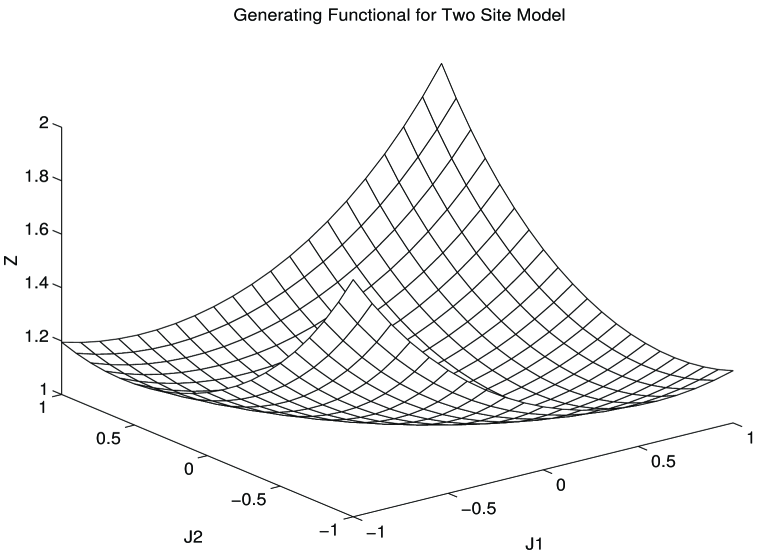
Figure 1: Galerkin Solution for M=1.0 and g=0.5

Figure 2: Residual as a function of the coupling for 4th order truncation

inner product of the $R$ with a test function, we are forming a linear combination of the SD equations organized by $\epsilon$. In other words, each Galerkin equation represents a different way of averaging the SD equations. This is how the problem of overdetermined equations is solved. The galerkin coefficients are not exact solutions, but averaged ones. Taking the limit $\epsilon\rightarrow 0$ forces the error due to the averaging into the higher order SD equations leaving the lower order ones exactly satisfied. Physically, taking this limit is reasonable since we are only interested in the behavior of $Z$ at the origin; physical Green’s functions are derivatives of $Z$ at $J=0$.

To see how well truncation approximates the theory, we examine the behavior of the residual as a function of the coupling. Notice that the the truncated SD equations had exact solutions in two limits, namely the free field limit and the infinite coupling limit where the theory breaks up into a collection of decoupled single sites. Recall that exact solutions corresponds to a vanishing residual. For the two site model truncated at 4th order, we have the following expression for the residual after the $\epsilon\rightarrow 0$ limit has been taken.

$$R=\frac{27G}{105G^{2}+1033G+550}\;J_{1}^{2}J_{2}-\frac{35G}{105G^{2}+1033G+550}\;J_{2}^{3}$$ (27)

where the coefficients of the residual measure the error in satisfying the individual SD equations.

Graphing the nonzero coefficients versus the coupling gives the expected behavior. At zero coupling, the error is zero, and rises to some maximum value as $g$ increases. Asymptotically, it falls off as $g$ approaches the strong coupling limit. While the magnitude of the error decreases at higher truncation order, the value of $g$ that gives the maximum error for a given truncation can vary and depends on the details of the system.

To examine convergence, we truncate at higher orders. The behavior of the residual is shown in the plots for the two site model where the $\epsilon\rightarrow 0$ limit has already been taken. We see that at higher orders $R$ becomes flatter about $J=0$ which is in the center of the plot. This indicates a reduction in the $L_{2}$ error which is measured as the integral of $R$ about the origin.

$$\parallel R\parallel_{2}=[\,\int_{-\epsilon}^{\epsilon}R^{2}\,d\vec{J}\,]^{1/2}$$ (28)

The flatter $R$, the smaller the integral of $R$ becomes.

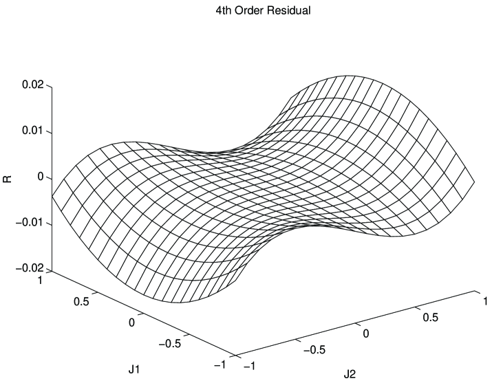
Figure 3: Error Profile for 4th order truncation

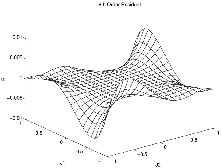
Figure 4: Error Profile for 6th order truncation

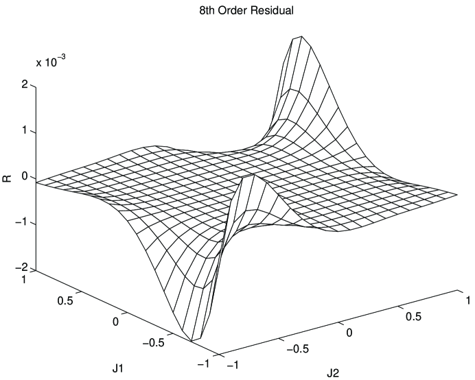
Figure 5: Error Profile for 8th order truncation

It is important to note that the $L_{2}$ norm of $R$ is an extremely powerful tool for controlling and measuring the error due to approximations. It is a general statement, independent of the choice of basis functions, of how well a given trial solutions approximates the differential equations. Specifically, it tells us how far we are from the exact solution. This is very much unlike other methods. For example, statistical errors can be calculated for Monte Carlo simulations, but in general, systematic errors can be difficult to quantify. Similarly, in variational calculations, since you never know the exact value of the ground state energy, in principle, you never know how close a given ansatz is to the exact ground state. This must often be inferred from other methods or from experiment.

4 Lattice Invariant Polynomials

In order to implement this method for larger systems, we need a systematic way to construct polynomials in the source variables that reflect the symmetries of our theory. A general term in our power series solution is represented by

$$a_{\{k1...kN\}}\;J^{k1}_{1}\ldots J^{kN}_{N}$$ (29)

where the subscripts index the sites at which the sources live and the $k_{i}$ are non-negative integer exponents. The coefficients $a_{\{k1...kN\}}$ are the Green’s functions of the theory and are required to be translation invariant. Therefore, we construct $Z_{T}$ to have the form

$$Z_{T}=\sum_{n,m}{a}_{n,m}{P}_{m,n}$$ (30)

where the $P_{m,n}$ transform into themselves under lattice symmetry operations. They are the invariant polynomials in the sources of order $n$ with $m$ invariant classes for a given order. The number of invariant classes for a given order depends on both the number of lattice sites and on the number of symmetry operations for a given lattice. For example, higher dimensional lattices have larger symmetry groups and will therefore have fewer independent invariants. These polynomials form a lattice invariant basis upon which we construct solutions for $Z$. In one-dimension, lattice field theories with periodic boundary conditions are invariant under translations and reflections of the underlying lattice. Such a lattice with $N$ sites is equivalent to an $N$-sided polygon, and the lattice symmetry group corresponds to the group of motions that transforms the polygon into itself. These are the dihedral groups $D_{N}$ of order $N$.

To construct polynomials invariant under $D_{N}$, we use the following shorthand [2] for the terms of our series

$$J_{1}^{k_{1}}\ldots J_{N}^{k_{N}}\rightarrow(k_{1}\ldots k_{N})$$ (31)

where $k_{i}$ is understood as the exponent associated with $J_{i}$. In this notion, performing symmetry operations is straightforward. Translations correspond to cyclic permutations of the exponents

$$(k_{1}\hskip 7.22743pt\ldots\hskip 7.22743ptk_{N})\rightarrow(k_{N}\hskip 7.22743ptk_{1}\hskip 7.22743pt\ldots\hskip 7.22743ptk_{N-1})\rightarrow\ldots$$ (32)

and reflections appear as inversions

$$(k_{1}\;\ldots\;k_{N})\;\rightarrow\;(k_{N}\;\ldots\;k_{1})$$ (33)

Given any single term, you can generate its entire associated invariant polynomial by applying the set of symmetry operations.

Now we present an algorithm to systematically generate all the invariant polynomials of a given degree. We try to identify an independent generator for each symmetry class. From these, we can construct the full polynomial $Z_{T}$ sorted into its invariant classes. Identifying these independent generators is a nontrivial problem. One method could involve forming all possible combinations of the $J_{i}$ at a given order, and then sorting the full set into its lattice invariant subsets. A “sieve algorithm” [2] can be constructed that establishes a criterion for sifting the independent representatives out of the full set.

An alternate approach is to construct the generators directly, without sorting through the full polynomial set. One recurring problem for all algorithms is that duplicate terms can be generated when terms have degenerate values for the $k_{i}$. To avoid this, some sorting is usually necessary. For the present algorithm, sorting is needed only for a restricted part of the full polynomial set. Each term in $Z_{T}$ for a given order $n$ and for $N$ sites is expressed as

$$(k1\hskip 7.22743ptk2\hskip 7.22743pt\ldots\hskip 7.22743ptkN)$$ (34)

This denotes some arrangement of the partitions of the integer $n$, distributed among the $k_{i}$. The other $N-n$ values are set to zero. The partition of an integer is defined as

$$a_{1}+a_{2}+...+a_{n}=n$$ (35)

with

$$a_{1}>a_{2}>\ldots>a_{n}>0.$$ (36)

Using this definition you can produce a hierarchy of polynomial terms like

(	$n$	0	0	0		$\ldots$	0)
(	$n-1$	1	0	0		$\ldots$	0)
(	$n-2$	2	0	0		$\ldots$	0)
(	$n-2$	1	1	0		$\ldots$	0)
	⋮
(	1	1	$\ldots$	1	0	$\ldots$	0)

Taking all possible permutations of these partition terms gives all the terms in the expansion for $Z$ at order $n$. In fact, this also generates many duplicate terms. Avoiding duplicates is one of the principle difficulties in constructing any algorithm.

Next, we ”bubble” the above partitions. This means permuting all members except the first while preserving the order of the nonzero elements.

(	$n-1$	1	0	0		$\ldots$	0)
(	$n-1$	0	1	0		$\ldots$	0)
	⋮
(	$n-1$	0	0	0		$\ldots$	1)

The word “bubble” suggests that you insert zeroes among the nonzero elements as if blowing bubbles between them. This bubbling procedure while keeping the first element fixed is the heart of the algorithm. Remember we are trying to construct generators directly. This means we are looking for ways to write down terms that are clearly not related by symmetry moves. Since symmetry moves correspond to cycles and inversions, fixing the first element breaks these symmetries. This guarantees that all of the independent generators are contained in the set of bubbled partitions.

There are special cases when the set of bubbled partitions does not contain all the generators. Since bubbling preserves the order of the nonzero elements, this excludes terms that do not have the descending hierarchy among the nonzero elements. For example on a four site lattice, taking all permutations of (4 3 2 0) includes terms like (4 2 3 0) which are missed under strict bubbling. An easy remedy is whenever you have two or more nondegenerate, nonzero elements, not including the first one, permute these elements before bubbling. In general, these permutations are only a minor part of the algorithm. Also note that not all bubbled partitions are independent. This is because a remnant of our lattice symmetry remains even after fixing the first element, namely reflections about site 1; the one we fixed. Therefore, we group terms that are related by reflections. After deleting the extra terms, the ones remaining are the independent generators.

Using these independent generators, you can recover their associated invariant polynomials by applying symmetry moves. Some of these terms, may either transform into themselves or into terms already present. When building a individual symmetric polynomial, you must check for duplicates. Some of the terms may transform into themselves or into terms already present in the individual polynomial. Since the invariant polynomials are generally small - the maximum size is equal to the total number of symmetry moves for the lattice ($2N$ for the dihedral group $D_{N}$), the number of checks is small and is done quickly.

The above algorithm for identifying the generators of the $D_{N}$ invariant polynomials generalizes immediately to the more complicated symmetry groups associated with higher dimensional lattices. In two-dimensions, there is a source variable $J_{(i,j)}$ living on each site of a square lattice and the power series must be invariant under all $2D$ symmetry moves.

$J_{1,N}$	$\ldots$	$J_{N,N}$
$\cdot$		$\cdot$
$\cdot$		$\cdot$
$J_{1,1}$	$\ldots$	$J_{N,1}$

In analogy with the $1D$ case, we represent a general term in our power series

$$J_{1,1}^{k_{(1,1)}}\hskip 7.22743pt\ldots\hskip 7.22743ptJ_{N,1}^{k_{(N,1)}}\hskip 7.22743pt\ldots\hskip 7.22743ptJ_{1,N}^{k_{(1,N)}}\hskip 7.22743pt\ldots\hskip 7.22743ptJ_{N,N}^{k_{(N,N)}}$$ (37)

as a 2D array of the integer exponents

$$\left|\begin{array}[]{ccc}k_{(1,N)}&\ldots&k_{(N,N)}\\ \cdot&&\cdot\\ k_{(1,1)}&\ldots&k_{(N,1)}\end{array}\right|$$

Here again, performing symmetry moves is straightforward. Translations with periodic boundary conditions corresponds to cyclic permutations of all rows or all columns. Similarly, reflections corresponds to inversions of all rows or all columns. Euclidean rotations are obtained by rotating the arrays by 90 degrees while reflections about the diagonal are performed as products of a rotation plus a reflection.

The algorithm we developed in the last section can be applied immediately. For a given order, we perform the partitions of $n$. If necessary, we permute nonzero elements. Then, we fill the 2D array from left to right beginning at the bottom left corner. Bubbling is performed by fixing the lower left corner element and inserting zeroes such that the nonzero elements are moved from left to right starting at the bottom row and moving to the top successively. As in the 1D case, even after fixing one element, there is still a remnant lattice symmetry in the set of bubbled partitions, namely reflections about the bottom left corner. Once this symmetry has been distilled, you are left with the independent generators. The full polynomial can be constructed by performing symmetry moves on these generators. Again, care must be taken in checking for duplicates within each individual polynomial. This procedure is identical for cubic and hypercubic lattices. Eventhough these groups can be large, they have been thoroughly studied and their elements tabulated [7].

5 Numerical Calculations

Now, we look at a variety of solutions to lattice $\phi^{4}$ field theory. Implementing the method numerically, we calculate Green’s functions and the corresponding mass-gaps for lattices in $D=2,3,4$. In $D=1$, reasonable large lattices can be examined. Results for these systems are given in [2],[1]. In higher dimensions, the rapid increase in complexity with the number of sites limits both linear size of the systems and the truncation orders available. In $D=2$, $8\times 8$ lattice models truncated at 4th order are possible on a workstation. But in $D=3,4$,

Figure 6: Propagator for 8x8 lattice with M=1.0, g=0.5

Figure 7: Propagator for $4^{3}$ lattice with M=1.0, g=0.5

Figure 8: Propagator for $2^{4}$ lattice with M=1.0, g=0.5

lattices larger than $4^{D}$ truncated at higher than 4th order are prohibitive. For each calculation, we compare our results against Monte Carlo simulations performed using the Metropolis algorithm.

Calculations with the Source Galerkin method are very clean and efficient, especially when compared to Monte Carlo. The complexity of calculations for polynomial basis functions scales with the total number of sites and the truncation order. It is independent of the dimensionality of the lattice and the form of the interaction. For polynomial interactions, the differential equations are always be linear. The bulk of a calculation involves a single matrix inversion for a given set of parameters. This is in contrast to Monte Carlo where many sweeps through the lattice are necessary to reduce statistical error. As the plots show, the Source Galerkin calculations show rapid convergence even at intermediate couplings and using only a fourth order polynomial.

6 An Alternative to the Galerkin Method

We have emphasized the flexibility of the Source Galerkin method with respect to choice of basis functions for our trial solution $Z_{T}$. Once we have a made a choice, we fit the approximation to a solution of the functional differential equations by using the Galerkin method. It is important to note that there is nothing fundamental about the Galerkin method. Its function is to minimize the error due approximation and force convergence to the exact solution in a controlled and systematic way. There are many ways to accomplish this, the Galerkin method being just one. Other procedures might be desirable based convenience. Here we present one such alternative.

Previously, we have emphasized that solving the lattice functional equations with a truncated power series leads to an overdetermined set of algebraic equations for the expansion coefficients. Because the equations cannot be solved exactly, the Galerkin method is used to find an average solution. In terms of the set of differential equations, the Galerkin method gives a “weak” solution where the error due to fitting the approximate solution is averaged over a hypercube centered at the origin of source space ranging from $+\epsilon$ to $-\epsilon$ in each direction. Since we want an especially good fit at the origin $(J=0)$, after the calculation we take $\epsilon\rightarrow 0$. In terms of the lattice SD equations, the combination of the Galerkin method and the $\epsilon\rightarrow 0$ limit gives a set of partially satisfied relations. For the 4th order truncated system, we had more equations than unknowns, but after $\epsilon\rightarrow 0$, all SD equations except for those at the highest untruncated order are solved exactly with the error being pushed successively to higher orders as the truncation increases.

With these observations in mind, consider some of the practical difficulties of the Galerkin method. The bulk of the computational effort involved in a Source Galerkin calculation is the inversion of a potentially very large matrix. In fact, the principle constraint of this approach is the size $N$ of the matrix that you can invert. Since for realistic systems these matrices must be inverted numerically and since they can become very large, it is critical that they be well-behaved.

For a numerical implementation of the method, this matrix is usually badly conditioned. Each row represents a different linear combination of all the SD equations where the Galerkin weightings depend heavily on $\epsilon$. But in order to perform the numerical extrapolation, we choose values of $\epsilon$ that are very small, typically $\epsilon\sim 1/10$. After integrating out the sources, the weightings can depend on a fairly high power of these small numbers. Since $\epsilon^{n}$ dominates over other numerical factors such as the coefficients in the SD equations and the system parameters $(M,g)$, variation between rows can be small. Since the lattice size and the truncation order is limited by the size of the matrix that can be inverted, we ideally would like sparse, well-conditioned matrices. Powerful algorithms exist for inverting sparse matrices that are not only efficient in terms of time and memory resources, but allow inversion of significantly larger matrices and with greater accuracy.

One possible method to accomplish this is to deal with the SD equations directly, bypassing the functional formulation and the Galerkin method. We know from looking at the solution to the SD equations that after using the Galerkin method and taking the limit $\epsilon\rightarrow 0$, all the low order equations are exactly satisfied, some of the highest order equations are exactly satisfied, and the remaining high order equations have some sort of average solution. It seems natural to ask why not solve the SD equations directly, and forget about power series, and integrating out the sources, and numerical extrapolations. Plus we obtain the practical advantage of sparse matrices.

In addition, this procedure considerably simplifies the fermion problem. In its original form, the Source Galerkin method is relative symmetric in its treatment of bosons and fermions, the only difference being that fermionic sources anticommute. While on the surface, this does not seem to be a problem, it does create a obstacle for constructing Galerkin solutions to the Grassmann differential equations. This problem must be solved by defining a modified form of Grassmann integration [3]. Using a scheme that attempts to solve the fermionic SD equations directly would be free not only of the practical handicaps of the boson method, but also would not require this modified integration.

We return to the two site model to examine these ideas. As a first attempt to solve the overdetermined equations, we notice that only one coefficient,$a_{4}$, in the set $\{a_{1},\ldots,a_{5}\}$ is constrained by more than one equation, namely the fourth and the fifth

$$\alpha\,a_{4}-2a_{5}-2a_{2} = 0.0247$$

$$\alpha\,a_{4}-2a_{3} = -0.0961.$$ (38)

To have a coefficient be constrained by an equation, we mean that the lattice KG operator acts directly on it in a particular SD equation. This operation is signaled by the factor of $\alpha$ multipling the coefficient. Also notice that the Source Galerkin method has pushed all the error into these two relations as indicated by the nonzero RHS. Furthermore, remember that for this model

$$a_{4} = \langle\phi_{1}^{3}\phi_{2}\rangle=\langle\phi_{1}\phi_{2}^{3}\rangle.$$

We have mentioned that the truncated SD equations are overdetermined. This is due to a symmetry mismatch between the lattice symmetric $Z$ and the individual differential source operators $\hat{D}_{i}$ which are symmetric only about site $i$. The individual $\hat{D}_{i}$ are not translation invariant. For the two site model, we use the single differential equation to constrain $Z$

$$\hat{D}_{i=1}\,Z=0.$$ (39)

Clearly, $a_{4}$, as defined above is not invariant under the symmetry group of $\hat{D}_{i=1}$. It is this tension that causes the additional equation for $a_{4}$ to be generated, and leave the set overdetermined.

We can, therefore, ask, if there are two equations for one unknown and both relations are only partially satisfied, then why not put all the error into one equation and solve the other one exactly. In other words, we solve a carefully chosen subset of the SD equations such that there is only one equation for each unknown. This is trivial way to calculate. We know what the lattice SD equations are. For example, two point function obeys

$$[\,2-(d^{+}_{i}+d^{-}_{i})+m^{2}\,]\,G_{2}(i,j)+g\,G_{4}(i,i,i,j)=\delta_{i,j}.$$ (40)

Higher order equations can be found easily. In large scale problems, the matrix becomes extremely sparse with no more that a few nonzero elements per row. Generation of the unknown Green’s functions is a simple exercise in combinatorics and symmetry identical to constructing invariant polynomials. Thus, we have found an approach with no sources, no integrals, and no $\epsilon$. In the end, we have a sparse matrix to invert.

Figure 9: Comparison of SD method with integral Galerkin with M=1.0, g=0.5

$|i-j|$	4th order		6th order		8th order		Monte Carlo
	SD	Galerkin	SD	Galerkin	SD	Galerkin
0	0.3274	0.3268	0.3592	0.3601	0.3481	0.3497	0.3426
1	0.0957	0.0948	0.1167	0.1177	0.1090	0.1096	0.1087
2	0.0278	0.0271	0.0383	0.0392	0.0344	0.0345	0.0329
3	0.0086	0.0081	0.0136	0.0143	0.0117	0.0117	0.0106
4	0.0045	0.0042	0.0080	0.0086	0.0066	0.0063	0.0057
mass-gap	1.2410	1.2647	1.1240	1.1189	1.1630	1.1649	1.1190
unknowns	34	34	160	160	600	600

Table 1: Comparison of SD, Galerkin, and MC for 8 site lattice

We performed several calculations on 10 site lattices, truncating at successive orders and comparing with both Monte Carlo and the integral Galerkin method. We see from the graph and the table that there is good agreement between the three approaches. Despite these results, it is uncertain if this approach will have problems for large systems at very high order. The reason is that by solving only a subset of the SD equations, we ignore more and more equations, the additional inconsistent ones, as we go to higher order. But these equations are relations that must be obeyed by the exact solution to the differential equations. By discarding, these equations, we have introduced an uncontrolled approximation. Ignoring these low order equations means that there is no guarantee that we will converge to the exact solution. As a practical matter, though, we rarely truncate above 4th or 6th order, so that this loss of a “rigorous” notion of convergence might not be a real problem, and in fact, may be a small price for the simplicity of this approach. For many examples, it has successfully captured many of the features of the truncated theory. In the next section, we outline how to define a rigorous notion of convergence in the lattice Green’s function approach. It will allow us to control the approximations in much the same way as the Galerkin method.

7 Flatness Criterion for Controlled Convergence

An important component of the Galerkin method is that it gives a rigorous, well-defined way to control the error due to the truncation approximation. At each level of truncation, Galerkin smoothed out the error, and by considering a sequence of successive truncations, we can improve our approximations and have a well-defined notion of convergence to the solution of the differential equations. Since we are proposing to dispense with at least the external trappings of the Galerkin method, we need to formulate a new way to control our approximations and enforce convergence to the correct solutions.

Recall that the Galerkin method, and in fact most spectral methods, are based on a trial solution to some differential equation. Since an exact solution is usually not available, some error is always present. Various approaches differ principally in how they deal with the problem of controlling and minimizing this error. The Galerkin method, for example, tries to minimize the area under the error function $R$. Effectively, it replaced the condition $R=0$ pointwise throughout the domain, which is only true for the exact solution, with $\int_{D}R\,[dx]=0$ i.e. the error vanishes on average across the domain. For problems in quantum field theory, we are only interested in minimization at the origin, so it is only the area of $R$ infinitesimally close to $J=0$ that is relevant. The question we ask is - are there other ways to enforce this condition of minimized area about zero without actually calculating integrals?

In the previous section, we developed an approach to find Green’s functions by solving a subset of the lattice SD equations. As mentioned, this introduces an uncontrolled approximation. To remedy this we would like to deal with the full set of equations. Of course, we know that the truncated SD equations can only be solved on average since they are overdetermined. If we can find some criterion to define what an average solution means in this SD context, then maybe we can retain the simplicity of the Green’s function approach, and in addition gain the rigorous notion of convergence that characterizes the Galerkin method. Towards this, first notice that the residual has the form of a Taylor’s series centered at the origin where the derivative coefficients are the SD equations which we would like to deal with directly.

$$R=\frac{dR}{dJ_{1}}|_{J=0}\,J_{1}+\frac{dR}{dJ_{2}}|_{J=0}\,J_{2}+\frac{d^{3}R}{dJ_{1}^{3}}|_{J=0}\,J_{1}+\frac{d^{3}R}{dJ_{1}^{2}dJ_{2}}|_{J=0}\,J_{1}^{2}J_{2}+\ldots$$ (41)

Obviously, the “flatter” $R$ is about the origin (i.e. has vanishing low order derivatives), the less area it will subtend. In fact, this is effectively what the Galerkin method does after $\epsilon\rightarrow 0$ as can be seen from the graphs of the two site residuals. At successively higher truncations, $R$ becomes flatter at the origin.

Figure 10: Flattening of the residual with higher order

We propose to control the error by invoking a “flatness criterion” to replace minimization of integrals. Of course, the flattest function that goes through the origin is $R=0$, but we know that $R$ cannot vanish because we do not have an exact solution. $R$ is necessarily a nontrivial function of the sources. Therefore, we zero as many of the low order derivatives of $R$ as possible, and then mix only the highest order derivatives in order to reduce the number of equations. Flattening $R$ about $J=0$ has exactly the same error content as minimizing the area and taking the $\epsilon\rightarrow 0$, only there are no integrals and no numerical extrapolations. We can make this method systematic by truncating $Z$ at successively higher orders and zeroing all derivatives except those at the highest untruncated order. As $R$ becomes flatter and flatter about $J=0$, the error is pushed into successively higher derivatives and $R$ smoothly approaches zero as the truncation goes to infinity.

Notice that to construct a notion of convergence and averaging, we appealed to $Z$ and the functional formulation to provide mathematical structure. But in practice, you never need to deal with $Z$ or with sources at all. The SD equations can be constructed quickly and independently of the partition function. It is even easy to determine what derivative of $R$ a particular equation corresponds to eventhough we never calculate $R$.

To obtain a complete theory, we must determine which equations to mix at the highest order and with what weightings, if any, to assign them. To do this, we can look for clues in the integral Galerkin method. In that approach, inner products of $R$ are taken with linearly independent test functions. These test functions act as projectors in the Galerkin function space and their precise functional form determines how the SD equations are mixed, and which equations become exact (or not) when $\epsilon\rightarrow 0$. In principle, there should be a map between a particular choice of test functions $\{T_{i}\}$ and how the SD equations are averaged. This is a nontrivial task because these rules are coded not only into the form of the inner product and the set of test functions, but also depend on the $\epsilon\rightarrow 0$ limit. At present only the loose form of these rules is known. This problem is being pursued and its resolution will be presented elsewhere.

8 Conclusions

In this paper, we have continued work on a new numerical method for quantum field theory called the Source Galerkin method. It is based on the differential formulation of quantum field theory in the presence of an external source. By examining the functional differential equations for a theory on a finite lattice, we obtain a set of coupled partial differential equations for the generating functional $Z$. For nonlinear field theories with polynomial interactions, the equations to solve are always linear. Once we have obtained $Z$, we can extract the Green’s functions by functional differentiation.

To construct solutions, we can expand $Z$ on any complete set of functions in the source variables $\{J\}$. A particularly simple choice is polynomial functions. We saw that these functions gave very rapid convergence even using low order polynomials. Calculations were efficient to perform and produced very clean numbers. The bulk of any calculation involved only a single matrix inversion. Due to computational complexity, polynomial basis functions are limited to small systems. A more general approach is required for large systems. We will have more to say about this in future communications.

Because our solutions for $Z$ are necessarily approximate, we found the Galerkin method very powerful for controlling error. It will fit any trial solution to a solution of the differential equations. This can be formulated in a systematic way, guaranteeing convergence to the exact solution. The residual function was especially useful for quantifying and controlling the error due to approximations. It is a very direct and precise measure of how well our approximations fit to the differential equations. This strong control of error should be contrasted against other methods especially Monte Carlo and variational techniques which rely on less precise determinations.

In another paper, we will show that the Source Galerkin method is especially powerful for fermion systems [3]. The fermionic formulation is identical except that the sources anticommute. Because this method is deterministic and allows for systematic approximations, it is very useful for examining these systems.

9 Acknowledgements

We would like to thank Stephen Hahn for useful discussions and for writing code used for the calculations in Section 6. In addition, we are indebted to Santiago Garcia for many discussions. GSG would like to thank Vance Faber for the Hospitality of C-3 at Los Alamos National Laboratory where some of this work was done.

References

- [1] S. Garcia, G.S. Guralnik, and J.W. Lawson, Physics Letters B322, (1994) 119
- [2] S. Garcia, Ph.D. Thesis, Brown University, (1992)
- [3] J.W. Lawson and G.S. Guralnik, Brown Preprint HET-954
- [4] S. Garcia and G.S. Guralnik, Brown Preprint HET-952
- [5] C.M. Bender, F. Cooper and L.M. Simmons, Jr, Phys. Rev. D39 2343 (1989).
- [6] C.A.J. Fletcher, Computational Galerkin Methods, Springer-Verlag, (1984)
- [7] J.E. Mandula, G. Zweig, J. Govaerts, Nucl PhysB 228, (1983) 91