Abstract

Using Operator Product Expansions and a graphical ansatz for the four-point function of the fundamental field $\phi^{\alpha}(x)$ in the conformally invariant $O(N)$ vector model, we calculate the next-to-leading order in $1/N$ values of the quantities $C_{T}$ and $C_{J}$. We check the results against what is expected from possible generalisations of the $C$- and $k$-theorems in higher dimensions and also against known three-loop calculations in a $O(N)$ invariant $\phi^{4}$ theory for $d=4-\epsilon$.

1 Introduction

Zamolodchikov’s $C$-theorem [1] states that there exist a quantity which is monotonously decreasing along the renormalisation group (RG) flow from the UV to the IR fixed points of unitary two-dimensional quantum field theories (QFT’s). At the fixed points, which correspond to conformal field theories (CFT’s) [2], this coincides with the Virasoro central charge and the conformal anomaly. Consequently, it has been suggested that a possible generalisation of the $C$-theorem in higher dimensions involves the conformal anomaly [3]. This is a promising yet not well worked out idea, (see [4] and references therein), since there does not seem to exist i.e. in four dimensions explicit CFT models other than the trivial bosonic, fermionic and spin-1 theories .

An alternative definition for the two-dimensional central charge is through the coefficient $C_{T}$ of the two-point function of the energy momentum tensor $T_{\mu\nu}(x)$. The latter has a unique form in any dimension $d$ [4], therefore it is conceivable that $C_{T}$ is related to the fixed point value of a possible generalisation of the $C$-function in three dimensions which is relevant for studies of statistical mechanical systems. Conveniently, in three dimensions there is a number of non-trivial CFT’s [6] and such an idea can be explicitly checked out.

In this letter we briefly report and discuss some of the results obtained in [7] for the Euclidean conformally invariant $O(N)$ vector model in $2<d<4$ (the physically relevant dimension is $d=3$). This model provides an example of a RG flow from an UV fixed point (free massless theory) to an IR one (non-trivial CFT) which can be explicitly studied. In [7] we calculated, among others, the value of $C_{T}$ at the non-trivial IR fixed point up to next-to-leading order in $1/N$ and we found it smaller that the value of $C_{T}$ at the UV fixed point in accordance with a possible generalisation of the $C$-theorem in higher dimensions.

Recently, the $k$-theorem [8] was proved for two-dimensional QFT’s stating that the Kac-Moody algebra level is the fixed point value of a quantity which is monotonously decreasing along the RG flow from the UV to the IR. A possible generalisation in higher dimensions of the Kac-Moody algebra level is through the coefficient $C_{J}$ of the two-point function of an internal symmetry conserved current $J_{\mu}(x)$. The latter has a unique form in any dimension $d$ [4]. In [7] we also calculated the value of $C_{J}$ up to next-to-leading order in $1/N$ at the IR fixed point of the $O(N)$ vector model and we found it smaller than the value of $C_{J}$ at the UV fixed point in accordance with a possible generalisation of the $k$-theorem.

2 General Framework for Calculations in the Conformally Invariant $O(N)$ Vector Model

The starting point of our calculations is the four-point function of the fundamental field [9] $\phi^{\alpha}(x)$, $\alpha=1,2,..,N$ in the $O(N)$ vector model. This, being dependent from conformal invariance on two variables [10] , can be written as [7]

$$\Phi^{\alpha\beta\gamma\delta}(x_{1},x_{2},x_{3},x_{4}) = H(\eta,x)\,F_{S}(u,v)\,\delta^{\alpha\beta}\delta^{\gamma\delta}$$ (1)

$${}+H(\eta,x)\,F_{V}(u,v)\,\frac{1}{2}(\delta^{\alpha\gamma}\delta^{\beta\delta}-\delta^{\alpha\delta}\delta^{\beta\gamma})$$

$${}+H(\eta,x)\,F_{T}(u,v)\,\frac{1}{2}(\delta^{\alpha\gamma}\delta^{\beta\delta}+\delta^{\alpha\delta}\delta^{\beta\gamma}-\frac{2}{N}\delta^{\alpha\beta}\delta^{\gamma\delta}),$$

where

$$F_{S}(u,v) = F(u,v)+\frac{1}{N}\left(F(\frac{1}{u},\frac{v}{u})+F(\frac{u}{v},\frac{1}{v})\right),$$

$$F_{V}(u,v) = F(\frac{1}{u},\frac{v}{u})-F(\frac{u}{v},\frac{1}{v}),\,\,\,\,\,F_{T}(u,v)=F(\frac{1}{u},\frac{v}{u})+F(\frac{u}{v},\frac{1}{v}),$$ (2)

$$H(\eta,x) = \frac{1}{(x_{12}^{2}x_{34}^{2}x_{13}^{2}x_{24}^{2}x_{14}^{2}x_{23}^{2})^{\frac{1}{3}\eta}},$$ (3)

and $F(u,v)=F(v,u)$ is an arbitrary function of the two invariant ratios

$$u=\frac{x_{12}^{2}x_{34}^{2}}{x_{13}^{2}x_{24}^{2}}\,\,\,\,\,\,\mbox{and}\,\,\,\,\,v=\frac{x_{12}^{2}x_{34}^{2}}{x_{14}^{2}x_{23}^{2}}.$$ (4)

Next, we make the basic assumption that the field algebra of a $O(N)$ invariant CFT is qualitatively similar to the field algebra of a free theory of $N$ massless scalar fields. Therefore, we write for the OPE of $\phi^{\alpha}(x)$ with itself

$$\phi^{\alpha}(x_{1})\phi^{\beta}(x_{2}) = C_{\phi}\frac{1}{x_{12}^{2\eta}}\delta^{\alpha\beta}+C^{\phi\phi O}(x_{12},\partial_{2})\,O(x_{2})\delta^{\alpha\beta}$$ (5)

$${}+\frac{g_{\phi\phi J}}{C_{J}}\,\frac{(x_{12})_{\mu}}{(x_{12}^{2})^{\eta-\mu+1}}\,J_{\mu}^{\alpha\beta}(x_{2})+\cdots$$

$${}-\frac{g_{\phi\phi T}}{C_{T}}\,\frac{(x_{12})_{\mu}(x_{12})_{\nu}}{(x_{12}^{2})^{\eta-\mu+1}}\,T_{\mu\nu}(x_{2})\,\delta^{\alpha\beta}+\cdots,$$

with $\mu=d/2$. Namely, the most singular terms as $x_{12}^{2}\rightarrow 0$ in the OPE (5) are assumed to be, apart from the contribution of the unit field, the coefficients of the $O(N)$ conserved vector current $J_{\mu}^{\alpha\beta}(x)$, of the (traceless) energy momentum tensor $T_{\mu\nu}(x)$ and also of some scalar field $O(x)$ with dimension $\eta_{o}$, $0<\eta_{o}<d$, whose two-point function in normalised as

$$\langle O(x_{1})\,O(x_{2})\rangle=C_{O}\frac{1}{x_{12}^{2\eta_{o}}}.$$ (6)

$C_{\phi}$ is the normalisation of the two-point function of $\phi^{\alpha}(x)$. The couplings $g_{\phi\phi J}$ and $g_{\phi\phi T}$ of the three-point functions $\langle\phi\phi J\rangle$ and $\langle\phi\phi T\rangle$ respectively can be found [7] (see also [11]) from the Ward identities to be

$$g_{\phi\phi J}=\frac{1}{S_{d}}C_{\phi},\,\,\,\,\,\,\,\,g_{\phi\phi T}=\frac{d\eta}{(d-1)S_{d}}C_{\phi},\,\,\,\,\,S_{d}=2\pi^{\frac{1}{2}d}/\Gamma({\textstyle{\frac{1}{2}}}d).$$ (7)

The coupling $g_{\phi\phi O}$ of the three-point function $\langle\phi\phi O\rangle$ and the field dimensions $\eta$, $\eta_{o}$ are dynamical parameters of the theory. The full OPE coefficient $C^{\phi\phi O}(x_{12},\partial_{2})$ can be found in a closed form using conformal integration techniques [7]. Substituting the OPE (5) into the four-point function (1) we obtain the most singular terms of the latter in the limit as $x_{12}^{2}$, $x_{34}^{2}\rightarrow 0$ independently. For completeness we give the form for the conformally invariant two-point functions of $T_{\mu\nu}(x)$ and $J_{\mu}^{\alpha\beta}(x)$ as [4]

$$\langle T_{\mu\nu}(x_{1})T_{\rho\sigma}(x_{2})\rangle = C_{T}\frac{I_{\mu\nu,\rho\sigma}(x_{12})}{x_{12}^{2d}},$$ (8)

$$\langle J_{\mu}^{\alpha\beta}(x_{1})J_{\nu}^{\gamma\delta}(x_{2})\rangle = C_{J}\frac{I_{\mu\nu}(x_{12})}{x_{12}^{2(d-1)}}\,(\delta^{\alpha\gamma}\delta^{\beta\delta}-\delta^{\alpha\delta}\delta^{\beta\gamma}),$$ (9)

with

$$I_{\mu\nu,\rho\sigma}(x) = \frac{1}{2}\Bigl{(}I_{\mu\rho}(x)I_{\nu\sigma}(x)+I_{\mu\sigma}(x)I_{\nu\rho}(x)\Bigl{)}{}-{}\frac{1}{d}\delta_{\mu\nu}\delta_{\rho\sigma},$$ (10)

$$I_{\mu\nu}(x) = \delta_{\mu\nu}-2\frac{x_{\mu}x_{\nu}}{x^{2}}.$$ (11)

After some algebra whose details are explained in [7] and using (8) and (9) above, the leading terms of $F_{S}(u,v)$ and $F_{V}(u,v)$ in (2) as $x_{12}^{2}$, $x_{34}^{2}\rightarrow 0$ are found to be

$$F_{S}(u,v) \equiv {\cal{F}}_{S}(Y,W)$$

$$=C_{\phi}^{2}W^{-\frac{2}{3}\eta}\!\!\!\!\!\!\!\!\!\!\!\!\!\! +\frac{g_{\phi\phi O}^{2}}{C_{O}}\,W^{\frac{1}{2}\eta_{o}-\frac{2}{3}\eta}\,\Bigg{(}1-\frac{\eta_{o}^{2}}{32(\eta_{o}+1)}Y^{2}+\frac{\eta_{o}^{3}}{16(\eta_{o}+1)(\eta_{o}+1-\mu)}\,W\,\Bigg{)}$$ (12)

$${}+\frac{g_{\phi\phi T}^{2}}{C_{T}}\,W^{\mu-1-\frac{2}{3}\eta}\,\Bigg{(}\frac{1}{4}\,Y^{2}-\frac{1}{d}\,W\Bigg{)}{}+\cdots,$$

$$F_{V}(u,v) \equiv {\cal{F}}_{V}(Y,W)=\frac{1}{2}\frac{g_{\phi\phi J}^{2}}{C_{J}}\,W^{\mu-1-\frac{2}{3}\eta}\,Y+\cdots.$$ (13)

We have used for convenience the two new independent variables

$$Y=1-\frac{v}{u} = 2\frac{1}{x_{24}^{2}}\left[(x_{12}\cdot x_{34})-2\frac{(x_{12}\cdot x_{24})(x_{34}\cdot x_{24})}{x_{24}^{2}}\right]+\cdots,$$ (14)

$$W=(uv)^{\frac{1}{2}} = \frac{x_{12}^{2}x_{34}^{2}}{x_{24}^{4}}+\cdots,$$ (15)

and the dots in (12), (13) stand for less singular terms in the limit $Y,W\rightarrow 0$.

It is clear now that having an expression for the four-point function (1) we can take suitable short distance limits and compare them with the above formulae (12) and (13). This would determine the values of the coupling $g_{\phi\phi O}$, the field dimensions $\eta$, $\eta_{o}$ and the wanted quantities $C_{T}$ and $C_{J}$. Such is the case for the UV fixed point of the $O(N)$ vector model, which corresponds to a free theory of $N$ massless scalar fields, when the full expression for the four-point function can be found using Wick’s theorem with elementary contraction the two-point function of $\phi^{\alpha}(x)$. This result indicates a graphical representation for $F_{f}(u,v)$ as shown in Fig.1, where the solid lines stand for the two-point function of $\phi^{\alpha}(x)$ and the subscript $f$ stands for “free field theory”.

Figure 1: The Graphical Expansion for $F_{f}(u,v)$

From $F_{f}(u,v)$ we find $F_{S,f}(u,v)$ and $F_{V,f}(u,v)$ as in (2) and we take their short distance limits as $Y$, $W\rightarrow 0$ independently. The resulting expressions are then compared with (12) and (13) and yield the values of the various parameters in the theory as

$$\eta=\frac{d}{2}-1,\,\,\,\,\,\eta_{o}=d-2,\,\,\,\,\,g_{\phi\phi O}^{2}=\frac{2}{N}C_{O}\,C_{\phi}^{2},$$

$$C_{T}=N\frac{d}{(d-1)S_{d}^{2}},\,\,\,\,\,C_{J}=\frac{2}{(d-2)S_{d}^{2}}.$$ (16)

The values of the various parameters given in (16) are in agreement with results given e.g. in [4] for the theory of $N$ massless scalar fields in any dimension $d$.

Next, we propose that a graphical expansion for a non-trivial $F(u,v)$ can be obtained by introducing a conformally invariant vertex into the theory. This vertex is assumed to describe the interaction of $\phi^{\alpha}(x)$ with an arbitrary scalar field ${\tilde{O}}(x)$, which is a $O(N)$ singlet and has dimension $\tilde{\eta}_{o}$ with $0<\tilde{\eta}_{o}<d$, whose two-point function we represent as a dashed line. The three-point function $\langle\phi\phi\tilde{O}\rangle$ has a coupling constant $g_{*}$ which has to be determined from the dynamics of the theory. Moreover, we assume that the amplitudes for $n$-point functions of $\phi^{\alpha}(x)$ with $n\geq 4$ in our non-trivial CFT are constructed in terms of skeleton graphs with no self-energy or vertex insertions and internal lines corresponding to the two-point functions of $\phi^{a}(x)$ and $\tilde{O}(x)$. Here we only consider graphs involving vertices corresponding to the fully amputated three-point function $\langle\phi\phi\tilde{O}\rangle$ which are graphically represented as dark blobs . Symmetry factors are determined as in the usual Feynman perturbation expansion . We denote by $F^{\tilde{\eta}_{o}}(u,v)$ the amplitude of interest in our graphical treatment of the four-point function (1). The first few graphs in the skeleton expansion for this amplitude in increasing order according to the number of vertices are displayed in Fig.2.

Figure 2: The Skeleton Graph Expansion for $H(x,\eta)\,F^{\tilde{\eta}_{o}}(u,v)$

The crucial consistency requirement regarding the present work is that amplitudes constructed according to graphical expansions such as the one in Fig.2, correspond to CFT’s having operator content in the agreement with the OPE ansatz (5) and are therefore compatible with amplitudes obtained by straightforward application of this ansatz on $n$-point functions. Without further input at this point we have no intrinsic means in estimating the magnitude of $g_{*}$ and hence we cannot hope to obtain a weak coupling expansion. However, on account of the $O(N)$ symmetry we subsequently see that the assumption $g_{*}^{2}=O(1/N)$ leads naturally to a well defined perturbation expansion in $1/N$ for the theory. Therefore, from now on we consider the theory for large $N$.

Details on the calculation of the amplitudes in Fig.2 are given in [7]. Here we just mention that these calculations are greatly facilitated by the use of the DEPP formula [12]

$$\int d^{d}x\frac{1}{(x_{1}-x)^{2a_{1}}(x_{2}-x)^{2a_{2}}(x_{3}-x)^{2a_{3}}}=\frac{U(a_{1},a_{2},a_{3})}{(x_{12}^{2})^{\mu-a_{3}}(x_{13}^{2})^{\mu-a_{2}}(x_{23}^{2})^{\mu-a_{1}}},$$ (17)

which is valid for $a_{1}+a_{2}+a_{3}=d$, with

$$U(a_{1},a_{2},a_{3})=\pi^{\mu}\frac{\Gamma(\mu-a_{1})\Gamma(\mu-a_{2})\Gamma(\mu-a_{3})}{\Gamma(a_{1})\Gamma(a_{2})\Gamma(a_{3})}.$$ (18)

In order to compare the formulae obtained from this calculation with the algebraically obtained expressions (12) and (13), we find that we need to identify the field $O(x)$ in the OPE ansatz (5), either with $\tilde{O}(x)$ or with the shadow field of the latter. The second possibility leads to a non-unitary theory which may be related to the free theory of $N$ massless scalars [7]. Here we are concerned with the first possibility above when we set $\eta_{o}=\tilde{\eta}_{o}$ and $g_{\phi\phi O}=g_{*}$. Expanding then the parameters of the theory in $1/N$ and having as only input that the leading order value of $\eta=\mu-1$, we obtain after some algebra

$$\eta = \mu-1+\frac{1}{N}\eta_{1},\,\,\,\,\,\,\,\,\eta_{1}=\frac{2\,\Gamma(2\mu-2)}{\Gamma(1-\mu)\Gamma(\mu)\Gamma(\mu+1)\Gamma(\mu-2)}\,,$$ (19)

$$\eta_{o} = 2+\frac{1}{N}\,\frac{4(2\mu-1)(\mu-1)}{\mu-2}\eta_{1}\,,$$ (20)

$$g_{\phi\phi O}^{2} = \frac{2}{N}\frac{\Gamma(2\mu-2)}{\Gamma(3-\mu)\Gamma^{3}(\mu-1)}\Bigl{(}1+\frac{1}{N}\,g_{1}\Bigl{)}\,,$$

$$g_{1} = -2\left(\frac{2\mu^{2}-3\mu+2}{\mu-2}{\cal{C}}(\mu)+\frac{8\mu^{3}-24\mu^{2}+21\mu-2}{2(\mu-1)(\mu-2)}\right)\eta_{1},$$ (21)

while the results for $C_{T}$ and $C_{J}$ read

$$C_{T} = \frac{Nd}{(d-1)S_{d}^{2}}\left(1+\frac{1}{N}\,C_{T,1}\right),\,C_{T,1}=-\left(\frac{2}{\mu+1}{\cal{C}}(\mu)+\frac{\mu^{2}+3\mu-2}{\mu(\mu-1)(\mu+1)}\right)\eta_{1},\,$$ (22)

$$C_{J} = \frac{2}{(d-2)S_{d}^{2}}\left(1+\frac{1}{N}\,C_{J,1}\right),\,C_{J,1}=-\frac{2(2\mu-1)}{\mu(\mu-1)}\eta_{1},\,$$ (23)

with ${\cal{C}}(\mu)=\psi(3-\mu)+\psi(2\mu-1)-\psi(1)-\psi(\mu)$, where $\psi(x)=\Gamma^{\prime}(x)/\Gamma(x)$.

3 Discussion of the Results

The next-to-leading order in $1/N$ values of $\eta$ and $\eta_{o}$ in (19) and (20) coincide with corresponding results in the Lagrangian formulation of the $O(N)$ vector model e.g. see [14] and references therein. The results (23) for $C_{J}$ and (21) for $g_{\phi\phi O}$ were first derived in [15] and [16] correspondingly. An expression for the next-to-leading order correction in $1/N$ for $C_{T}$ was given in [16] but it is different from our result (22). We explain below why our result (22) is believed to be correct.

Our results (19)-(23) give the values of the dynamical parameters at the non-universal IR fixed point of the $O(N)$ vector model in $2<d<4$ . It is believed that this IR fixed point is connected through the RG flow with an UV one, which corresponds to a free (Gaussian) theory of $N$ massless scalars. However, this RG flow is nonperturbative over the parameter space since it cannot be seen in a weak coupling expansion but only in the context of the $1/N$ expansion. It is also worth noting that the UV Gaussian theory has a field of dimension $d-2$ while the IR non-trivial theory has a field of dimension $2+O(1/N)$. Therefore, for $N\rightarrow\infty$ and e.g. $d=3$ they seem to be different theories since the have different field content. However, the duality property discussed in [7] may relate these two theories at the expense of unitarity.

In Fig.3 we plot $C_{T,1}$ and $C_{J,1}$ for $2<d<4$ and by virtue of (22) and (23) we see that, at least to the order in $1/N$ considered here, $C_{T}$(UV)$>C_{T}$(IR) and $C_{J}$(UV)$>C_{J}$(IR). This is in accord with a possible generalisation of the $C$- and $k$-theorems in higher dimensions requiring $C_{T}$ and $C_{J}$ to be the fixed point values of the $C$- and $k$-functions respectively.

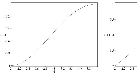
Figure 3: $C_{T,1}$ and $C_{J,1}$ for $2<d<4$.

In two dimensions the $C$-function counts, properly normalised, the massless degrees of freedom in the theory on a particular length scale [3]. Adopting such an interpretation for the $C$-function in higher dimensions we may normalise $C_{T}$ in (16) to $N$ e.g. the number of massless scalar fields. It is well known [17] that the existence of a non-trivial IR fixed point in the $O(N)$ vector model for $2<d<4$ is an indication for the symmetry breaking pattern $O(N)\rightarrow O(N-1)$ in the theory. That is, the IR critical point separates the $O(N)$ symmetric phase having $N$ massive modes, from the $O(N-1)$ symmetric one with $N-1$ massless Goldstone bosons and one massive mode. Hence, at this fixed point the potential $C$-function, properly normalised, should have $N-1$ as lower bound. Indeed, for $2<d<4$ we see from the first graph in Fig.3 that $N-1<C_{T}$(IR) is satisfied which is another test for the validity of our result (22).

The $k$-function on the other hand is connected with the internal symmetry of the theory i.e. in a theory with no such symmetry a $k$-function does not exist. If an internal symmetry remains unbroken along the RG flow from the UV to the IR fixed point we expect that $k$(UV)$=k$(IR). We may therefore interpret the $k$-function as counting the amount of internal symmetry in the theory on a particular length scale. At the fixed points the number of conserved currents, i.e. $N(N-1)/2$ for a $O(N)$ invariant theory, may be taken as a quantity which counts the amount of internal symmetry. Hence, we expect that the $k$-function at the IR fixed point of the $O(N)$ vector model for $2<d<4$, normalised to 1 in the $O(N)$ symmetric phase, should satisfy $1-(2/N)<k$(IR). Indeed, from (16), (23) and the second graph in Fig. 3 we see that $1-(2/N)<C_{J}$(IR) is remarkably satisfied.

Another crucial test for our results (22) and (23) is to compare them with known results in the context of $\epsilon$-expansion when $\epsilon=4-d>0$. In four dimensions, if the theory is defined for a background metric $g_{\mu\nu}$ and has a gauge field $A_{\mu}^{\alpha}$ coupled to the conserved vector current, even for a conformal theory there is a trace anomaly [4, 18]

$$g^{\mu\nu}\langle T_{\mu\nu}\rangle=-\beta_{a}F-\kappa{\textstyle{\frac{1}{4}}}F_{\mu\nu}^{\alpha}F^{\alpha,\mu\nu}+\cdots,$$ (24)

where $F$ is the square of the Weyl tensor and terms which are irrelevant here are neglected. The quantities $\beta_{a}$ and $\kappa$ can be perturbatively calculated and for a $O(N)$ invariant renormalisable field theory with ${\textstyle{\frac{1}{24}}}g\left(\phi^{2}\right)^{2}$ interaction, a three-loop calculation yields [19]

$$\beta_{a} = -\frac{1}{16\pi^{2}}\frac{N}{120}\Bigl{(}1-\frac{5}{108}(N+2)u^{2}\Bigl{)},$$ (25)

$$\kappa = \frac{1}{3}\frac{1}{16\pi^{2}}\,R\,\Bigl{(}1-\frac{1}{12}(N+2)u^{2}\Bigl{)},$$ (26)

where $u=g/16\pi^{2}$ with $g$ the renormalised coupling and $\mbox{tr}(t^{\alpha}t^{\beta})=-\delta^{\alpha\beta}R$. For the adjoint representation of $O(N)$ we have $(t^{\alpha\beta})^{\gamma\delta}=-(\delta^{\alpha\gamma}\delta^{\beta\delta}-\delta^{\alpha\delta}\delta^{\beta\gamma})$ and $R=2$. The results of our previous work [4] show that for a conformal theory when $d=4$

$$C_{T}=-\frac{640}{\pi^{2}}\beta_{a}\,\,\,\,\,,\,\,\,\,\,C_{J}=\frac{6}{\pi^{2}}\kappa.$$ (27)

In general we suppose that we may write $C_{T}(\epsilon,u_{*})$, $C_{J}(\epsilon,u_{*})$ where $u_{*}$ is the critical coupling. The free or Gaussian field theory results in (16) correspond to $C_{T,f}=C_{T}(\epsilon,0)$ and $C_{J,f}=C_{J}(\epsilon,0)$ while (22) and (23) give $C_{T}(0,u)$ and $C_{J}(0,u)$. Using then (25) and (26) with $u_{*}=3\epsilon/(N+8)+O(\epsilon^{2})$ [21] gives the leading corrections in the $\epsilon$-expansion

$$C_{T} = C_{T,f}\Bigl{(}1-\frac{5}{12}\frac{N+2}{(N+8)^{2}}\epsilon^{2}+O(\epsilon^{3})\Bigl{)},$$ (28)

$$C_{J} = C_{J,f}\Bigl{(}1-\frac{3}{4}\frac{N+2}{(N+8)^{2}}\epsilon^{2}+O(\epsilon^{3})\Bigl{)}.$$ (29)

As $d\rightarrow 4$ we see from (19) that $\eta_{1}\sim\epsilon^{2}/4$ and then we can easily show that out results (22) and (23) agree correspondingly with (28) and (29), something which is a remarkable independent check for their validity at least up to the order considered here.

Finally, we note that it was shown in [11] that $C_{T}$ parametrises universal finite size effects of statistical systems at their critical points in two dimensions which provides a natural method for its measurement both numerically and experimentally. For $d>2$, although Cardy [11] has pointed out that $C_{T}$ may be in principle measurable, the finite scaling of the free energy is parametrised [23] by a universal number $\tilde{c}$ whose relation with $C_{T}$ is not clear. Sachdev [24] has calculated $\tilde{c}$ for the $O(N)$ vector model to leading order in $1/N$ for $d=3$ and found it to be a rational number however different from the leading order in $1/N$ value for $C_{T}$ . Using our results (22) and (23) we obtain for $d=3$

$$C_{T}|_{d=3} = N\frac{3}{2S_{3}^{2}}\Bigl{(}1-\frac{1}{N}\frac{40}{9\pi^{2}}\Bigl{)},$$ (30)

$$C_{J}|_{d=3} = \frac{2}{S_{3}^{2}}\Bigl{(}1-\frac{1}{N}\frac{32}{9\pi^{2}}\Bigl{)}.$$ (31)

With our normalisation $C_{T}$ has to be multiplied by $S_{d}^{2}/2$ to agree with the corresponding quantity in [24], and then we can answer by virtue of (30) part of the question addressed in that reference: $C_{T}$ does not seem to be a rational number for finite $N$ in three dimensions.

Acknowledgments

I am indebted to Professor John Cardy for a very illuminating discussion.

References

- [1] A. B. Zamolodchikov, JETP Lett. 43 (1986) 730
-
[2]
B. Schroer, Lett. Nuovo Cimento, 2 (1971) 867,
J. Polchinski, Nucl. Phys. B303 (1988) 226 - [3] J. L. Cardy, Phys. Lett. B215 (1988) 749
- [4] H. Osborn and A. C. Petkou, Ann. Phys. 231 (1994) 311
- [5] N. Seiberg, Nucl. Phys. B435 (1995) 129
-
[6]
J. A. Gracey, Z. Phys. C59 (1993) 243; Int. J. Mod. Phys. A9 (1994)
727;
M. Ciuchini, Phys. Lett. 339B (1994) 252;
W. Chen, Y. Makeenko and G. Semenoff, Ann. Phys. 228 (1993) 525 - [7] A. C. Petkou, “Conserved Currents, Operator Product Expansions and Consistency relations in the Conformally Invariant Vector Model for ”, DAMTP preprint 94/12, hep-th/9410093, unpublished
- [8] X. Vilasis-Cardona, Nucl. Phys. B435 (1995) 735
- [9] A. B. Zamolodchikov and Al. B. Zamolodchikov, Sov. Sci. Rev. A. Phys. vol 10 (1989) 269
- [10] P. Ginsparg, in “Champs, Cordes et Phénomènes Critiques”, (E. Brézin and J. Zinn-Justin eds.) North Holland , Amsterdam 1989
- [11] J. L. Cardy Nucl. Phys. B270 (1987) 355
-
[12]
M. D’Eramo, G. Parisi and L. Peliti, Lett. Nuovo Cimento, 2 (1971)
878,
K. Symanzik, Lett. Nuovo Cimento, 3 (1972) 734 -
[13]
S. Ferrara, R. Gatto, A. F. Grillo and G. Parisi, Lett. Nuovo Cimento
4 (1972) 115,
S. Ferrara, A. F. Grillo and G. Parisi, Lett. Nuovo Cimento 5 (1972) 147 - [14] K. Lang and W. Rühl, Nucl. Phys. B377 (1992) 371
- [15] K. Lang and W. Rühl, Nucl. Phys. B402 (1993) 573
- [16] K. Lang and W. Rühl, Z. Phys. C61 (1994) 495
-
[17]
A. M. Polyakov, Gauge Fields and Strings (Harwood Academic,
New York 1978);
B. Rosenstein, B. J. Warr and S. H. Park, Nucl. Phys. B336 (1990) 435 - [18] N. Birrel and P. C. W. Davies, Quantum Fields in Curved Space (Cambridge University Press, Cambridge, 1982)
- [19] I. Jack and H. Osborn, Nucl. Phys. B234 (1984) 331; B343 (1990) 647
- [20] A. Cappelli, D. Friedan and J. I. Latorre, Nucl. Phys. B352 (1991) 616
- [21] J. Zinn-Justin, Quantum Field Theory and Critical Phenomena, 2nd ed. (Clarendon, Oxford, 1993)
-
[22]
I. Affleck, Phys. Rev. Lett. 56 (1986) 746,
H. W. J. Blöte, J. L. Cardy and M. P. Nightingale, Phys. Rev. Lett. 56 (1986) 742 - [23] A. H. Castro Neto and E. Fradkin, Nucl. Phys. B400 (1993) 525
- [24] S. Sachdev, Phys. Lett. 309B (1993) 285