The matrix sine-Gordon theory, a matrix generalization of the well-known sine-Gordon theory, is studied. In particular, the $A_{3}$-generalization where fields take value in $SU(2)$ describes integrable deformations of conformal field theory corresponding to the coset $SU(2)\times SU(2)/SU(2)$. Various classical aspects of the matrix sine-Gordon theory are addressed. We find exact solutions, solitons and breathers which generalize those of the sine-Gordon theory with internal degrees of freedom, by applying the Zakharov-Shabat dressing method and explain their physical properties. Infinite current conservation laws and the Bäcklund transformation of the theory are obtained from the zero curvature formalism of the equation of motion. From the Bäcklund transformation, we also derive exact solutions as well as a nonlinear superposition principle by making use of the Bianchi’s permutability theorem.

1 Introduction

The sine-Gordon theory is the most well-known example of relativistic integrable field theories in 1+1 dimensions. Exact solutions, topological solitons and breathers, are known and various applications of these solutions have been made in the study of a wide range of physical systems. However, in many cases, such an application has been made after a truncation of the physical systems, i.e. suppressing all degrees of freedom except one scalar field, so that the sine-Gordon theory becomes an effective description of the reduced system. In this regard, it is desirable to have generalizations of the sine-Gordon theory with additional degrees of freedom whereas the integrability of the theory is maintained to provide exact solutions. One such example is the so-called complex sine-Gordon theory which appeared in the description of the relativistic vortex motion in a superfluid[1], in a treatment of O(4) nonlinear sigma model[2] and more recently in the context of conformal field theory[3]. In the complex sine-Gordon theory, the scalar field is complex valued so that the phase factor becomes an additional physical degree. Other types of nonabelian generalization of the sine-Gordon theory, carrying extra internal degrees, have been considered recently in the context of integrable deformation of the coset conformal field theory[4], particularly in the case of the critical Ising model deformed by $\Phi_{(2,1)}$ and $\Phi_{(3,1)}$ operators[5]. In fact, to each classical Lie algebras, there exist nonabelian generalizations of the sine-Gordon theory which admit a positive definite kinetic energy when certain criteria of the sl(2) embedding are met[6]. The complex sine-Gordon theory and the critical Ising model deformed by $\Phi_{(2,1)}$ operator arise as first two examples in these generalizations which correspond to the Lie algebra $B_{2}$ and $A_{3}$ respectively.

In this Paper, we study in detail the $A_{3}$-generalization of the sine-Gordon theory, which we call “the matrix sine-Gordon theory”, at the classical level. At the quantum level, this theory may be regarded as an integrable deformation of a minimal model[8] corresponding to the coset $SU_{N}(2)\times SU_{N}(2)/SU_{2N}(2)$, in particular the deformation of the critical Ising model by the energy operator $\Phi_{(2,1)}$ if the level $N=1$. We demonstrate the classical integrability of the theory by deriving infinite current conservation laws from the zero curvature formalism of the equation of motion. The Bäcklund transformation is also obtained from the zero curvature formalism, and using the Bianchi’s theorem of permutability[9] a nonlinear superposition principle is derived for the solutions of the matrix sine-Gordon theory. Exact solutions, solitons and breathers which generalize those of the sine-Gordon theory, are obtained by making use of the Zakharov-Shabat dressing method[10]. These solutions carry internal degrees of freedom which affect the scattering process. Two soliton solutions for the soliton(antisoliton) - soliton(antisoliton) scattering is given explicitly in terms of parameters $u$ and $\theta$ which describe the relative velocity of solitons and their relative internal directions respectively. It is shown that the nonabelian effect which is controlled by the parameter $\theta$ makes solitons less repulsive for larger $\theta$ while the scattering time of far removed solitons does not depend on $\theta$. An explicit form of nonabelian breather solution is also given in terms of both energy configuration and internal components with parameters $v$ and $\theta$. The breather solution is a bound state of soliton and antisoliton which oscillates in time with angular frequency $2\sqrt{-\kappa}v/\sqrt{1+v^{2}}$. As $\theta$ increases, the breathing mode of the potential energy configuration diminishes and at $\theta=\pi$, it becomes completely breathless! However, the internal components still oscillate at $\theta=\pi$ which keeps the static potential energy configuration. Alternative derivation of one and two soliton solutions are also given using the Bäcklund transformation and the nonlinear superposition principle.

The plan of the Paper is the following; in Sec.2, we define the model in terms of the gauged Wess-Zumino-Witten functional and address issues on the gauge invariance and the gauge fixing. We present the zero curvature formalism of the equation of motion for the model and from which, derive infinite current conservation laws thereby demonstrating the integrability of the model. In Sec.3, exact solutions, N solitons and breathers, are derived rigorously by making use of the dressing method. A pictorial description of these solutions is given and their physical meaning is discussed. Sec.4 deals with the Bäcklund transformation and the nonlinear superposition principle and Sec.5 is a discussion.

2 The Model

We introduce the matrix sine-Gordon theory from the context of conformal field theory and its integrable deformations. The action principle for the G/H-coset conformal field theory may be given in terms of the gauged Wess-Zumino-Witten(WZW) functional[11], which in light-cone variables is

$$S(g,A,\bar{A})=S_{WZW}(g)+{1\over 2\pi}\int\mbox{Tr}(-A\bar{\partial}gg^{-1}+\bar{A}g^{-1}\partial g+Ag\bar{A}g^{-1}-A\bar{A})$$ (1)

and $S_{WZW}(g)$ is the action of group G WZW model

$$S_{WZW}(g)=-{1\over 4\pi}\int_{\Sigma}\mbox{Tr }g^{-1}\partial gg^{-1}\bar{\partial}g-{1\over 12\pi}\int_{B}\mbox{Tr }\tilde{g}^{-1}d\tilde{g}\wedge\tilde{g}^{-1}d\tilde{g}\wedge\tilde{g}^{-1}d\tilde{g}\ .$$ (2)

$\tilde{g}$ is an extension of a map $g:\Sigma\rightarrow G$ to a three-dimensional manifold $B$ with boundary $\Sigma,\ \ \tilde{g}|_{\partial B}=g$, and the connection fields $A,\bar{A}$ gauge the anomaly free subgroup H of G. Here, we take the diagonal embedding of H in $G_{L}\times G_{R}$, where $G_{L}$ and $G_{R}$ denote left and right group actions by multiplication $(g\rightarrow g_{L}gg_{R}^{-1})$, so that Eq.(1) is invariant under the vector gauge transformation; $g\rightarrow hgh^{-1}$ with $h:\Sigma\rightarrow$H. In particular, the minimal unitary series in conformal field theory arise from the restriction to the coset, $(SU(2)_{L}\times SU(2)_{N})/SU(2)_{L+N}$, where integers $L,N$ denote the level of the Kac-Moody algebra[8]. In this case, the full theory is given formally by functional integrals,

$$\int[dg_{1}][dg_{2}][dA][d\bar{A}]\exp{iI_{0}(g_{1},g_{2},A,\bar{A})}$$ (3)

where

$$I_{0}(g_{1},g_{2},A,\bar{A})=LS_{WZW}(g_{1},A,\bar{A})+NS_{WZW}(g_{2},A,\bar{A})$$ (4)

and $A,\bar{A}$ gauge simultaneously the diagonal subgroups of $SU(2)\times SU(2)$.

The matrix sine-Gordon theory is defined as a massive deformation of the minimal series with $L=N$ which, at the action level, is adding a potential term to the action,

$$I(g_{1},g_{2},A,\bar{A},\kappa)=I_{0}(g_{1},g_{2},A,\bar{A})-{N\kappa\over 2\pi}\int\mbox{Tr}(g^{-1}_{1}g_{2}+g^{-1}_{2}g_{1}),$$ (5)

where $\kappa$ is a coupling constant. Note that the potential term is invariant under the similarity transform; $g_{1}\rightarrow sg_{1}s^{-1},\ g_{2}\rightarrow sg_{2}s^{-1}$ so that the vector gauge invariance of the action is maintained. In the convention of coset conformal field theory, the potential term transforms at the classical level as (doublet, singlet) so that it corresponds to the integrable perturbation of minimal series by the operator $\Phi_{(2,1)}$[12]. In this Paper, we focus only on the classical aspect of the theory so that the level $N$ is irrelevant. In order to understand the vacuum structure, we parameterize $g^{-1}_{1}g_{2}$ by

$$g^{-1}_{1}g_{2}=\exp(i\phi\hat{\sigma})\ ,\ \hat{\sigma}=\sum_{i=1}^{3}a_{i}\sigma_{i}$$ (6)

where $\sigma_{i}$ are Pauli matrices and the coefficients $a_{i}$ are normalized to one, $\sum_{i=1}^{3}a_{i}a_{i}=1$. Then, the potential becomes

$$V={N\kappa\over 2\pi}\mbox{Tr}(g^{-1}_{1}g_{2}+g^{-1}_{2}g_{1})={2N\kappa\over\pi}\cos\phi\ .$$ (7)

If the coupling constant $\kappa<0$, $V$ possesses degenerate vacua at $\phi=2n\pi$ for integer $n$ so that $g^{-1}_{1}g_{2}=1$ or for any arbitrary $g_{1}=g_{2}$ valued in $SU(2)$. Note that a specific vacuum is characterized only by the integer $n$ independently of $a_{i}$. The degeneracy of the vacuum allows soliton solutions which interpolate different vacuua. The explicit solutions will be found in Sec.3 and Sec.4. The topological soliton numbers are defined by the difference $\Delta n=n_{1}-n_{2}$ of integer values of two interpolating vacuua. If $\kappa>0$, degenerate vacuua occur at $\phi=(2n+1)\pi$ for integer $n$ so that $g^{-1}_{1}g_{2}=-1$, or for any arbitrary $g_{1}=-g_{2}$. From now on, we will restrict ourselves to the $\kappa<0$ case only. $\kappa>0$ case will be discussed in Sec.5.

The classical equation of motion arising from the action Eq.(5) is

$$[\ \partial+g^{-1}_{1}\partial g_{1}+g^{-1}_{1}Ag_{1}\ ,\ \bar{\partial}+\bar{A}\ ]-\kappa(g^{-1}_{1}g_{2}-g^{-1}_{2}g_{1})=0$$

$$[\ \partial+g^{-1}_{2}\partial g_{2}+g^{-1}_{2}Ag_{2}\ ,\ \bar{\partial}+\bar{A}\ ]+\kappa(g^{-1}_{1}g_{2}-g^{-1}_{2}g_{1})=0$$ (8)

whereas variations of the action with respect to $A$ and $\bar{A}$ give rise to the constraint equation,

$$-\bar{\partial}g_{1}g^{-1}_{1} + g_{1}\bar{A}g^{-1}_{1}-\bar{\partial}g_{2}g^{-1}_{2}+g_{2}\bar{A}g^{-1}_{2}-2\bar{A}=0$$

$$g^{-1}_{1}\partial g_{1} + g^{-1}_{1}Ag_{1}+g^{-1}_{2}\partial g_{2}+g^{-1}_{2}Ag_{2}-2A=0\ .$$ (9)

The constraint equation in Eq.(9), when combined with the equation of motion in Eq.(8), results in the flatness condition of $A$ and $\bar{A}$,

$$\partial\bar{A}-\bar{\partial}A+[A,\bar{A}]=0,$$ (10)

which reflects the vector gauge invariance of the action. In the following, we consider two types of different gauge fixing. Assume that the underlying manifold $\Sigma$ is the flat two-dimensional Minkowski space $R^{1+1}$. Then the flatness of $A$ and $\bar{A}$ allows us to choose a “nonlocal gauge”;

$$A=\bar{A}=0.$$ (11)

The equation of motion in the nonlocal gauge becomes

$$\bar{\partial}(g^{-1}_{1}\partial g_{1})+\kappa(g^{-1}_{1}g_{2}-g^{-1}_{2}g_{1})=0$$

$$\bar{\partial}(g^{-1}_{2}\partial g_{2})-\kappa(g^{-1}_{1}g_{2}-g^{-1}_{2}g_{1})=0$$ (12)

whereas the constraint equation becomes

$$\bar{\partial}g_{1}g^{-1}_{1}+\bar{\partial}g_{2}g^{-1}_{2}=0\ ,\ g^{-1}_{1}\partial g_{1}+g^{-1}_{2}\partial g_{2}=0\ .$$ (13)

In the abelian limit, where $g_{1}=\exp{i\phi_{1}}\sigma_{1},\ g_{2}=\exp{i\phi_{2}\sigma_{1}}$, the constraint equation may be solved locally by $\phi_{1}=\phi=-\phi_{2}$ so that the equation of motion in terms of $\phi$ becomes precisely the sine-Gordon equation. However, for $g_{1},g_{2}$ valued in $SU(2)$, the constraint equation in general can not be solved locally. Consequently, in the nonlocal gauge, a local parametrization solving the constraint is not possible as in the abelian case.

Nevertheless, there exists another type of gauge fixing, so-called “the unitary gauge”[13], which allows a local parametrization solving the constraint in the following sense; for any given $g_{1}$ and $g_{2}$, one may bring $g_{2}$ into a form $g_{2}=\exp(i\phi\sigma_{3})$ via the similarity transform; $g_{1}\rightarrow sg_{1}s^{-1},g_{2}\rightarrow sg_{2}s^{-1}$ for some $s$. Thus, the scalar function $\phi$ parameterizes the equivalence classes of $g_{2}$ with the equivalence relation given by the similarity transform. The remaining $U(1)$ gauge symmetry which leaves $g_{2}$ invariant may be used to fix $g_{1}$ to give the unitary gauge;

$$g_{1}=\pmatrix{ue^{-i\phi}&~{}&i\sqrt{1-uu^{*}}e^{i\phi}\cr i\sqrt{1-uu^{*}}e^{-i\phi}&~{}&u^{*}e^{i\phi}}\ ,\ g_{2}=\pmatrix{e^{i\phi}&0\cr 0&e^{-i\phi}}\ .$$ (14)

In this gauge, the constraint equation can be solved explicitly for $A$ and $\bar{A}$ in terms of $u$ and $\phi$,

$$A=\pmatrix{a&-b^{*}\cr b&-a}\ ,\ \ \ \bar{A}=\pmatrix{\bar{a}&-\bar{b}^{*}\cr\bar{b}&-\bar{a}}$$ (15)

where

$$b = {-ie^{-2i\phi}\partial u\over 2\sqrt{1-uu^{*}}}-{i\partial u+i\partial u^{*}\over 8\sqrt{1-uu^{*}}\sin^{2}\phi}$$

$$a = {(e^{2i\phi}u^{*}-u)\partial u^{*}-(e^{-2i\phi}u-u^{*})\partial u\over 4(1-uu^{*})}-{(u-u^{*})(\partial u+\partial u^{*})\over 16(1-uu^{*})\sin^{2}\phi},$$ (16)

and

$$\bar{b} = {\bar{\partial}u^{*}\over 4\sqrt{1-uu^{*}}\sin^{2}\phi}-{ie^{2i\phi}\bar{\partial}u^{*}-ie^{-2i\phi}\bar{\partial}u\over 8\sqrt{1-uu^{*}}\sin^{2}\phi}$$

$$\bar{a} = -i\bar{\partial}\phi-{(e^{2i\phi}u^{*}-u)\bar{\partial}u^{*}-(e^{-2i\phi}u-u^{*})\bar{\partial}u\over 4(1-uu^{*})}+{(u-u^{*})(\bar{\partial}u+\bar{\partial}u^{*})\over 16(1-uu^{*})\sin^{2}\phi}.$$ (17)

Then the flatness condition Eq.(10) resolves into the equations of motion for $u$, $u^{*}$ and $\phi$. These equations are related to those of the nonlocal gauge by the following association; if we solve Eq.(10) in terms of holonomies, $A=h^{-1}\partial h$ and $\bar{A}=h^{-1}\bar{\partial}h$, then $g_{1},g_{2}$ of the nonlocal gauge are related to those of the unitary gauge by

$$g_{1}^{N}=hg_{1}^{U}h^{-1}\ ,\ g_{2}^{N}=hg_{2}^{U}h^{-1}\ .$$ (18)

For the rest of the Paper, we will restrict ourselves only to the nonlocal gauge. Translation of subsequent results into the unitary gauge can be readily made by the association in Eq.(18).

In order to understand the integrability of the matrix sine-Gordon theory, we consider the linear $4\times 4$ matrix equations with a spectral parameter $\lambda$,

$$L_{1}(\lambda)\Psi \equiv (\partial+U_{0}-\lambda T)\Psi=0$$

$$L_{2}(\lambda)\Psi \equiv (\bar{\partial}+{\bar{\cal A}}+{1\over\lambda}V_{1})\Psi=0$$ (19)

where

$$U_{0}={\cal G}^{-1}\partial{\cal G}+{\cal G}^{-1}{\cal A}{\cal G}\ ,\ V_{1}={\cal G}^{-1}\bar{T}{\cal G}\ ,\ T=i\kappa\Sigma\ ,\ \bar{T}=i\Sigma$$ (20)

and

$${\cal G}\equiv\pmatrix{g_{1}&0\cr 0&g_{2}}\ ,\ {\cal A}\equiv\pmatrix{A&0\cr 0&A}\ ,\ {\bar{\cal A}}\equiv\pmatrix{\bar{A}&0\cr 0&\bar{A}}\ ,\ \Sigma\equiv\pmatrix{0&1\cr 1&0}$$ (21)

with each entries being $2\times 2$ matrices. The matrix sine-Gordon equation arises precisely as an integrability condition, $[L_{1}(\lambda)\ ,\ L_{2}(\lambda)]=0$, of the linear equation for any $\lambda$. The advantage of the linear equation with a spectral parameter $\lambda$ is that it allows a systematic way to construct infinite conserved currents. In addition, exact solutions can be obtained from the linear equation which we consider in Sec.3. In order to find conserved currents, we solve the linear equation iteratively by setting

$$\Phi\equiv\Psi\exp(-\lambda Tz)=\sum_{m=0}^{\infty}\lambda^{-m}\Phi_{m}\ ;\ \Phi_{0}=1$$ (22)

so that the $m$-th order equation in the nonlocal gauge is

$$\partial\Phi_{m} + U_{0}^{\bot}\Phi-[T,\Phi_{m+1}]=0$$

$$\bar{\partial}\Phi_{m} + V_{1}\Phi_{m-1}=0$$

$$U_{0}^{\bot} \equiv {1\over 2}\pmatrix{g^{-1}_{1}\partial g_{1}-g^{-1}_{2}\partial g_{2}&0\cr 0&g^{-1}_{2}\partial g_{2}-g^{-1}_{1}\partial g_{1}}\ .$$ (23)

In accordance with the initial value $\Phi_{0}=1$, $\Phi_{m}$ can be appropriately parametrized by

$$\Phi_{2m}\equiv\pmatrix{P_{2m}&0\cr 0&S_{2m}}\ ,\ \Phi_{2m+1}\equiv\pmatrix{0&P_{2m+1}\cr S_{2m+1}&0}\ ;\ m\geq 0\ .$$ (24)

This brings Eq.(23) into a component form,

$$\bar{\partial}P_{m+1} + ig^{-1}_{1}g_{2}S_{m}=0$$

$$\bar{\partial}S_{m+1} + ig^{-1}_{2}g_{1}P_{m}=0$$

$$\partial P_{m} + g^{-1}_{1}\partial g_{1}P_{m}=i\kappa(P_{m+1}-S_{m+1})$$

$$\partial S_{m} + g^{-1}_{2}\partial g_{2}S_{m}=i\kappa(S_{m+1}-P_{m+1})\ ,$$ (25)

which we solve iteratively with initial values $P_{0}=S_{0}=1$,

$$P_{m+1}-S_{m+1} = {1\over 2i\kappa}[\partial(P_{m}-S{m})+g^{-1}_{1}\partial g_{1}(P_{m}+S_{m})]$$

$$P_{m+1}+S_{m+1} = -\int d\bar{z}(ig^{-1}_{1}g_{2}S_{m}+ig^{-1}_{2}g_{1}P_{m})-\int dzg^{-1}_{1}\partial g_{1}(P_{m+1}-S_{m+1})\ .$$ (26)

In particular,

$$P_{1} = {1\over 2i\kappa}g^{-1}_{1}\partial g_{1}-{1\over 2i\kappa}\int dz(g^{-1}_{1}\partial g_{1})^{2}-{i\over 2}\int d\bar{z}(g^{-1}_{1}g_{2}+g^{-1}_{2}g_{1})$$

$$S_{1} = -{1\over 2i\kappa}g^{-1}_{1}\partial g_{1}-{1\over 2i\kappa}\int dz(g^{-1}_{1}\partial g_{1})^{2}-{i\over 2}\int d\bar{z}(g^{-1}_{1}g_{2}+g^{-1}_{2}g_{1})\ .$$ (27)

With iterative solutions of the linear equation, we find that the consistency of Eq.(25), $\partial\bar{\partial}P_{m}=\bar{\partial}\partial P_{m}$ and $\partial\bar{\partial}S_{m}=\bar{\partial}\partial S_{m}$, gives rise to two sets of current conservation laws;

$$\bar{\partial}J^{(1)}_{m} + \partial\bar{J}^{(1)}_{m+2}=0$$

$$\bar{\partial}J^{(2)}_{m} + \partial\bar{J}^{(2)}_{m+2}=0\ ;\ \ m\geq 0$$ (28)

where

$$\bar{J}^{(1)}_{m} = ig^{-1}_{1}g_{2}S_{m}$$

$$J^{(1)}_{m+2} = \partial P_{m+1}=-g^{-1}_{1}\partial g_{1}P_{m+1}+i\kappa(S_{m+1}-P_{m+1})$$

$$\bar{J}^{(2)}_{m} = ig^{-1}_{2}g_{1}P_{m}$$

$$J^{(2)}_{m+2} = \partial S_{m+1}=g^{-1}_{1}\partial g_{1}S_{m+1}+i\kappa(P_{m+1}-S_{m+1})\ .$$ (29)

The subscript $m$ of the current $J_{m}$ denotes the conformal spin in the massless limit, or it simply counts the order of the derivatives. In particular, the $m=0$ case is the energy-momentum conservation,

$$\bar{\partial}T_{\pm}+\partial\Theta_{\pm}=0,$$ (30)

where

$$T_{+} \equiv i\kappa(J^{(1)}_{2}+J^{(2)}_{2})=(g^{-1}_{1}\partial g_{1})^{2}$$

$$\Theta_{+} \equiv i\kappa(\bar{J}^{(1)}_{0}+\bar{J}^{(2)}_{0})=-\kappa(g^{-1}_{1}g_{2}+g^{-1}_{2}g_{1})$$ (31)

while the other half of the conserved currents are

$$T_{-} \equiv i\kappa(J^{(1)}_{2}-J^{(2)}_{2})=\partial(g^{-1}_{1}\partial g_{1})$$

$$\Theta_{-} \equiv i\kappa(\bar{J}^{(1)}_{0}-\bar{J}^{(2)}_{0})=-\kappa(g^{-1}_{1}g_{2}-g^{-1}_{2}g_{1})\ .$$ (32)

It is interesting to observe that $T_{-}$ in the abelian limit becomes $T_{-}=\partial^{2}\phi$ which is precisely the term added to improve the energy-momentum tensor in the Feigin-Fuchs construction[14]. Another type of conserved currents arises from the invariance of the matrix sine-Gordon theory under the parity transform,

$$z\leftrightarrow\bar{z}\ \ \mbox{ and }\ \ g_{1}\leftrightarrow g^{-1}_{1}\ ,\ g_{2}\leftrightarrow g^{-1}_{2}\ .$$ (33)

This leads to the parity conjugate pair of conserved currents which, together with currents in Eq.(29), constitute a complete set of conserved currents of the matrix sine-Gordon theory. For example, the parity conjugate of the energy-momentum is

$$\bar{T}_{+} = (\bar{\partial}g_{1}g^{-1}_{1})^{2}\ ,\ \bar{\Theta}_{+}=-\kappa(g_{1}g^{-1}_{2}+g_{2}g^{-1}_{1})$$ (34)

and

$$\bar{T}_{-}=-\bar{\partial}(\bar{\partial}g_{1}g^{-1}_{1})\ ,\ \bar{\Theta}_{-}=-\kappa(g_{1}g^{-1}_{2}-g_{2}g^{-1}_{1})\ .$$ (35)

3 Dressing Method and Soliton Solutions

In this section, we give a detailed account of the derivation of soliton solutions. We follow the dressing method of Zakharov and Shabat[10] and obtain nontrivial soliton solutions from the trivial one by employing the Riemann problem technique with zeros[15]. In Sec.4, we give an alternative method based on the Bäcklund transformation and obtain soliton solutions by direct integration. We first give a brief review on the dressing method. For later purpose, we rewrite the linear equation in the nonlocal gauge by making a similarity transform of Eq.(19) by the matrix $Q$,

$$Q=Q^{-1}\equiv{1\over\sqrt{2}}\pmatrix{1&1\cr 1&-1}$$ (36)

such that

$$(\partial+U_{0}^{{}^{\prime}}-\lambda T^{{}^{\prime}})\Psi^{{}^{\prime}}=0\ ,\ (\bar{\partial}+{1\over\lambda}V_{1}^{{}^{\prime}})\Psi^{{}^{\prime}}=0$$ (37)

where

$$\Psi^{{}^{\prime}} = Q\Psi Q^{-1}$$

$$U_{0}^{{}^{\prime}} = QU_{0}Q^{-1}=\pmatrix{0&g_{1}^{-1}\partial g_{1}\cr g_{1}^{-1}\partial g_{1}&0}$$

$$V_{1}^{{}^{\prime}} = QV_{1}Q^{-1}={i\over 2}\pmatrix{g_{1}^{-1}g_{2}+g_{2}^{-1}g_{1}&g_{2}^{-1}g_{1}-g_{1}^{-1}g_{2}\cr g_{1}^{-1}g_{2}-g_{2}^{-1}g_{1}&-g_{1}^{-1}g_{2}-g_{2}^{-1}g_{1}}$$ (38)

and

$$T^{{}^{\prime}}=QTQ^{-1}={i\kappa}\pmatrix{1&0\cr 0&-1}\ ,\ \bar{T}^{{}^{\prime}}=Q{\bar{T}}Q^{-1}={i}\pmatrix{1&0\cr 0&-1}.$$ (39)

In the following, we drop the prime for convenience without causing any confusion. The dressing method is a systematic way to obtain nontrivial solutions from a trivial one. In our case, we take the vacuum as a trivial solution of Eq.(37),

$$g_{1}=g_{2}=1\ \mbox{ and }\Psi=\Psi^{o}\equiv\exp(\lambda Tz-\lambda^{-1}\bar{T}\bar{z})\ .$$ (40)

Let $\Gamma$ be a closed contour or a contour extending to infinity on the complex plane of the parameter $\lambda$. Consider the matrix function $\Phi_{+}(z,\bar{z},\lambda)$ which is analytic with $n$ simple poles $\mu_{1},...,\mu_{n}$ inside $\Gamma$ and $\Phi_{-}(z,\bar{z},\lambda)$ analytic with $n$ simple zeros $\lambda_{1},...,\lambda_{n}$ outside $\Gamma$. We assume that none of these zeros lies on the contour $\Gamma$ and $\Psi^{0}(\Psi^{0})^{-1}=(\Phi_{-})^{-1}\Phi_{+}=1$ for $\lambda\neq\mu_{i},\lambda_{i}\ ;\ i=1,...,n$. We normalize $\Phi_{+},\Phi_{-}$ by $\Phi_{+}|_{\lambda=\infty}=\Phi_{-}|_{\lambda=\infty}=1$. Differentiating $\Psi^{o}\Psi^{o-1}=(\Phi_{-})^{-1}\Phi_{+}=1$ with respect to $z$ and $\bar{z}$, one can easily see that

$$\partial\Phi_{+}\Phi_{+}^{-1}+\lambda\Phi_{+}T\Phi_{+}^{-1} = \partial\Phi_{-}\Phi_{-}^{-1}+\lambda\Phi_{-}T\Phi_{-}^{-1}$$

$$\bar{\partial}\Phi_{+}\Phi_{+}^{-1}-{1\over\lambda}\Phi_{+}\bar{T}\Phi_{+}^{-1} = \bar{\partial}\Phi_{-}\Phi_{-}^{-1}-{1\over\lambda}\Phi_{-}\bar{T}\Phi_{-}^{-1}.$$ (41)

Since $\Phi_{+}(\Phi_{-})$ is analytic inside (outside) $\Gamma$, we find that the matrix functions $\tilde{U}_{0}$ and $\tilde{V}_{1}$, defined by

$$\tilde{U}_{0}\equiv-\partial\Phi\Phi^{-1}-\Phi\lambda T\Phi^{-1}+\lambda T\ ;\ \tilde{V}_{1}\equiv-\lambda\bar{\partial}\Phi\Phi^{-1}+\Phi\bar{T}\Phi^{-1}$$ (42)

where $\Phi=\Phi_{+}$ or $\Phi_{-}$ depending on the region, become independent of $\lambda$. Also, $\tilde{\Psi}\equiv\Phi\Psi^{o}$ satisfies the linear equation;

$$(\partial+\tilde{U}_{0}-\lambda T)\tilde{\Psi}=0\ ,\ (\bar{\partial}+{1\over\lambda}\tilde{V}_{1})\tilde{\Psi}=0\ .$$ (43)

The identification $\tilde{\Psi}=\Psi$ and $\tilde{U}_{0},\ \tilde{V}_{1}$ with respect to $U_{0},V_{1}$ in Eq.(38), $\tilde{U}_{0}$ and $\tilde{V}_{1}$ then provide nontrivial $n$-soliton solutions.

In making such an identification, the specific form of $U_{0}$ and $V_{1}$ imposes restrictions on $\Psi$ which in certain cases may be solved algebraically. For example, the anti-unitarity of $U_{0}$ and $V_{1}$ imposes restrictions on $\Psi$ and $\Phi$ which may be complied with

$$\Psi^{\dagger}(\lambda)=\Psi^{-1}(\lambda^{*})\ ,\ \Phi^{\dagger}(\lambda)=\Phi^{-1}(\lambda^{*})\ .$$ (44)

These are not the most general expression giving the anti-unitary $U_{0}$ and $V_{1}$, however we assume Eq.(44) since they suffice for our purpose of deriving soliton solutions. In order to construct the matrix function $\Phi$ for the soliton solutions, we take the ansätze for $\Phi$ and $\Phi^{-1}$,

$$\Phi=1+\sum_{\alpha=1}^{M}({A^{\alpha}\over\lambda-\nu_{\alpha}})\ ,\ \Phi^{-1}=1+\sum_{\alpha=1}^{M}({B^{\alpha}\over\lambda-\mu_{\alpha}}),$$ (45)

where the matrix functions $A^{\alpha}(z,\bar{z}),B^{\alpha}(z,\bar{z})$ are to be determined. Since the identity; $\Phi\Phi^{-1}=1$ and Eq.(42) should hold for any $\lambda$, they require respectively algebraic and differential relations among $A^{\alpha}$ and $B^{\alpha}$. These relations can be obtained through the evaluation of residues of both equations at $\lambda=\mu_{\alpha},\nu_{\alpha}$. For instance, the residues of the equation $\Phi\Phi^{-1}=1$ gives rise to

$$A^{\alpha}+A^{\alpha}\sum_{\beta=1}^{M}({B^{\beta}\over\nu_{\alpha}-\mu_{\beta}})=0\ ,\ B^{\alpha}+\sum_{\beta=1}^{M}({A^{\beta}\over\mu_{\alpha}-\nu_{\beta}})B^{\alpha}=0,$$ (46)

while those of Eq.(42) lead to

$$A^{\alpha}D_{1,2}(\nu_{\alpha})[1+\sum_{\beta=1}^{M}({B^{\beta}\over\nu_{\alpha}-\mu_{\beta}})]=0\ ,\ [1+\sum_{\beta=1}^{M}({A^{\beta}\over\mu_{\alpha}-\nu_{\beta}})]D_{1,2}(\mu_{\alpha})B^{\alpha}=0$$ (47)

where

$$D_{1}(\lambda)\equiv\partial-\lambda T\ ,\ D_{2}(\lambda)\equiv\bar{\partial}+{1\over\lambda}\bar{T}.$$ (48)

In order to solve Eqs.(46) and (47), we assume that $A^{\alpha}_{ij}=s^{i}_{\alpha}t^{j}_{\alpha}\ ,\ B^{\alpha}_{ij}=n^{i}_{\alpha}m^{j}_{\alpha}$ where $s^{i}_{\alpha},t^{i}_{\alpha},n^{i}_{\alpha},m^{i}_{\alpha}$ are two by two matrices with $i=1,2$. Then, Eqs.(46) and (47) changes into

$$\sum_{j=1}^{2}t_{\alpha}^{j}[\delta^{ji}+\sum_{\beta=1}^{M}{n_{\beta}^{j}m_{\beta}^{i}\over\nu_{\alpha}-\mu_{\beta}}]=0\ ,\ \sum_{i=1}^{2}[\delta^{ji}+\sum_{\beta=1}^{M}{s_{\beta}^{j}t_{\beta}^{i}\over\mu_{s}-\nu_{\beta}}]n_{s}^{i}=0$$ (49)

and

$$D_{1,2}(\mu_{\alpha})n_{\beta}=0\ ,\ t_{\beta}D_{1,2}(\nu_{\alpha})=0\ ,$$ (50)

where we understand $t_{\beta}\partial$ and $t_{\beta}\bar{\partial}$ as $-\partial t_{\beta}$ and $-\bar{\partial}t_{\beta}$. Note that $n_{\alpha}$ and $t_{\alpha}$ can be solved in terms of arbitrary constant vectors $\bar{n}_{\alpha}$ and $\bar{t}_{\alpha}$,

$$n_{\alpha}^{i}=\sum_{j=1}^{2}[\Psi^{o}(\mu_{\alpha})]^{ij}\bar{n}^{j}_{\alpha}\ ,\ t^{i}_{\alpha}=\sum_{j=1}^{2}[\Psi^{o}(\nu_{\alpha})^{-1}]^{ji}\bar{t}^{j}_{\alpha}\ ,$$ (51)

while $m_{\alpha}$ and $s_{\alpha}$ can be obtained in terms of $t_{\alpha}$ and $n_{\alpha}$ by solving the linear algebraic equation (49) such that

$$m^{i}_{\alpha}=-\sum_{\beta=1}^{M}V^{-1}_{\alpha\beta}t^{i}_{\beta}\ ,\ s^{i}_{\alpha}=\sum_{\beta=1}^{M}n^{i}_{\beta}V^{-1}_{\beta\alpha}\ ,$$ (52)

where

$$V_{\alpha\beta}\equiv\sum_{j=1}^{2}{t_{\alpha}^{j}n_{\beta}^{j}\over\nu_{\alpha}-\mu_{\beta}}\ .$$ (53)

$V^{-1}$ is defined by $\sum_{\beta=1}^{M}V^{-1}_{\alpha\beta}V_{\beta\gamma}=\delta_{\alpha\gamma}1$ where $1$ is the $2\times 2$ unit matrix. The unitarity condition Eq.(44) requires that

$$\mu_{\alpha}=\nu^{*}_{\alpha}\ \ \mbox{ and }\ \ A^{\alpha\dagger}=B^{\alpha}(\ \ \mbox{ or }\ \ t^{i\dagger}_{\alpha}=n^{i}_{\alpha},\ s^{i\dagger}_{\alpha}=m^{i}_{\alpha}\ ).$$ (54)

Consequently,

$$\bar{t}^{i\dagger}_{\alpha}=\bar{n}^{i}_{\alpha}\ ,\ (V^{-1}_{\beta\alpha})^{\dagger}=-V^{-1}_{\alpha\beta}\ .$$ (55)

Further specification of $t_{\alpha}$ and $n_{\alpha}$ arises from the identification; $U_{0}=\tilde{U}_{0},V_{1}=\tilde{V}_{1}$, in Eq.(42). Since Eq.(42) holds for any $\lambda$, we combine Eq.(42) and (45) and take the $\lambda\rightarrow\infty$ limit to obtain

$$-U_{0}=\sum_{\alpha}(A^{\alpha}T+TB^{\alpha})=i\kappa\sum_{\alpha}\pmatrix{s^{1}_{\alpha}t^{1}_{\alpha}+n^{1}_{\alpha}m^{1}_{\alpha}&-s^{1}_{\alpha}t^{2}_{\alpha}+n^{1}_{\alpha}m^{2}_{\alpha}\cr s^{2}_{\alpha}t^{1}_{\alpha}-n^{2}_{\alpha}m^{1}_{\alpha}&-s^{2}_{\alpha}t^{2}_{\alpha}-n^{2}_{\alpha}m^{2}_{\alpha}}\ .$$ (56)

Note that the (block)-diagonal part vanishes identically due to the equality

$$s^{i}_{\alpha}t^{i}_{\alpha}+n^{i}_{\alpha}m^{i}_{\alpha}=n^{i}_{\beta}(V^{-1})_{\beta\alpha}t^{i}_{\alpha}-n^{i}_{\alpha}(V^{-1})_{\alpha\beta}t^{i}_{\beta}=0$$ (57)

which agrees with $U_{0}$. The off-diagonal part gives rise to

$$g^{-1}_{1}\partial g_{1}=-i\kappa(-s^{1}_{\alpha}t^{2}_{\alpha}+n^{1}_{\alpha}m^{2}_{\alpha})=2i\kappa\sum_{\alpha,\beta}n^{1}_{\beta}V^{-1}_{\beta\alpha}t^{2}_{\alpha}=2i\kappa\sum_{\alpha,\beta}Z^{-1}_{\alpha\beta},$$ (58)

or

$$g_{1}^{-1}\partial g_{1}=-i\kappa(s^{2}_{\alpha}t^{1}_{\alpha}-n^{2}_{\alpha}m^{1}_{\alpha})=-2i\kappa\sum_{\alpha,\beta}n^{2}_{\alpha}V^{-1}_{\alpha\beta}t^{1}_{\beta}=-2i\kappa\sum_{\alpha,\beta}{\tilde{Z}}^{-1}_{\alpha\beta}\ ,$$ (59)

where $Z_{\alpha\beta}$ and ${\tilde{Z}}_{\alpha\beta}$ are defined by

$$Z_{\alpha\beta} \equiv {(t^{2}_{\beta})^{-1}t^{1}_{\beta}+n^{2}_{\alpha}(n^{1}_{\alpha})^{-1}\over{\nu_{\beta}-\mu_{\alpha}}}={N^{\dagger}_{\beta}+N^{-1}_{\alpha}\over\mu^{*}_{\beta}-\mu_{\alpha}}$$

$${\tilde{Z}}_{\alpha\beta} \equiv {n^{1}_{\alpha}(n^{2}_{\alpha})^{-1}+(t^{1}_{\beta})^{-1}t^{2}_{\beta}\over{\nu_{\beta}-\mu_{\alpha}}}={N_{\alpha}+N^{-1\dagger}_{\beta}\over\mu^{*}_{\beta}-\mu_{\alpha}}=-Z^{\dagger}_{\beta\alpha}$$

$$N_{\beta} \equiv n^{1}_{\beta}(n^{2}_{\beta})^{-1}=\exp(2\Delta_{\beta})\bar{n}^{1}_{\beta}(\bar{n}^{2}_{\beta})^{-1}\equiv\exp(2\Delta_{\beta})\bar{N}_{\beta}$$

$$\Delta_{\beta} \equiv i\kappa\mu_{\beta}z-{i\bar{z}\over\mu_{\beta}}\$$ (60)

and we have used the unitarity condition Eq.(54). The last step in Eq.(58) (similarly Eq.(59)) can be checked easily by using $K^{2}_{\alpha}\equiv\sum_{\beta}V^{-1}_{\alpha\beta}t^{2}_{\beta}$ so that

$$t^{2}_{\beta}=\sum_{\alpha}V_{\beta\alpha}K^{2}_{\alpha}=t^{2}_{\beta}\sum_{\alpha}{(t^{2}_{\beta})^{-1}t^{1}_{\beta}+n^{2}_{\alpha}(n^{1}_{\alpha})^{-1}\over\nu_{\beta}-\mu_{\alpha}}n^{1}_{\alpha}K^{2}_{\alpha}=t^{2}_{\beta}\sum_{\alpha}Z_{\alpha\beta}n^{1}_{\alpha}K^{2}_{\alpha}\ .$$ (61)

Thus, the identification with $U_{0}$ through Eqs.(58) and (59) imposes restrictions on $Z_{\alpha\beta}$ such that

$$\sum_{\alpha,\beta}Z^{-1}_{\alpha\beta}=-\sum_{\alpha,\beta}{\tilde{Z}}^{-1}_{\alpha\beta}=\sum_{\alpha,\beta}Z^{\dagger-1}_{\alpha\beta}.$$ (62)

On the other hand, the $V_{1}$ part in the $\lambda\rightarrow 0$ limit of the linear equation, gives rise to

$$V_{1}=\Phi\bar{T}\Phi^{-1}|_{\lambda=0}\ \mbox{ or }\ \Phi|_{\lambda=0}\bar{T}=V_{1}\Phi|_{\lambda=0}\ .$$ (63)

In components, they are

$$g_{1}^{-1}g_{2}=-(\Phi_{12}+\Phi_{22})(\Phi_{12}-\Phi_{22})^{-1}$$ (64)

or

$$g_{1}^{-1}g_{2}=-(\Phi_{11}+\Phi_{21})(\Phi_{21}-\Phi_{11})^{-1}$$ (65)

where $\Phi_{ij}$ denote $2\times 2$ block components of $\Phi|_{\lambda=0}$. We will see below that the two expressions for $g_{1}^{-1}g_{2}$ in Eqs.(64) and (65) are indeed equivalent when the condition Eq.(62) is satisfied. If we define

$$Y_{\alpha\beta}\equiv{1+N^{\dagger}_{\alpha}N_{\beta}\over 1-\mu_{\beta}/\mu^{*}_{\alpha}}\ ,$$ (66)

Eqs.(64) and (65) become

$$g_{1}^{-1}g_{2} = -(\Phi_{12}+\Phi_{22})(\Phi_{12}-\Phi_{22})^{-1}$$ (67)

$$= \biggl{[}1-\sum_{\alpha}{(s^{1}_{\alpha}+s^{2}_{\alpha})t^{2}_{\alpha}\over\nu_{\alpha}}\biggr{]}\biggl{[}1-\sum_{\alpha}{(-s^{1}_{\alpha}+s^{2}_{\alpha})t^{2}_{\alpha}\over\nu_{\alpha}}\biggr{]}^{-1}$$

$$= \biggl{[}1-\sum_{\alpha,\beta}(1+N_{\beta})(Y^{-1})_{\beta\alpha}\biggr{]}\biggl{[}1-\sum_{\alpha,\beta}(1-N_{\beta})(Y^{-1})_{\beta\alpha}\biggr{]}^{-1},$$

and

$$g_{1}^{-1}g_{2} = -(\Phi_{11}+\Phi_{21})(\Phi_{21}-\Phi_{11})^{-1}$$ (68)

$$= \biggl{[}1-\sum_{\alpha}{(s^{1}_{\alpha}+s^{2}_{\alpha})t^{1}_{\alpha}\over\nu_{\alpha}}\biggr{]}\biggl{[}1+\sum_{\alpha}{(-s^{1}_{\alpha}+s^{2}_{\alpha})t^{1}_{\alpha}\over\nu_{\alpha}}\biggr{]}^{-1}$$

$$= \biggl{[}1-\sum_{\alpha,\beta}(1+N_{\beta})(Y^{-1})_{\beta\alpha}N^{\dagger}_{\alpha}][1+\sum_{\alpha,\beta}(1-N_{\beta})(Y^{-1})_{\beta\alpha}N^{\dagger}_{\alpha}\biggr{]}^{-1}\ .$$

These are M-soliton solutions of the matrix sine-Gordon theory. In the following, we give an explicit expression for M=1 and 2.

M=1; 1-soliton

For M=1, we have

$$Z=-\tilde{Z}^{\dagger}={N^{\dagger}+N^{-1}\over\mu^{*}-\mu}$$ (69)

and Eq.(62) for M=1, $Z^{-1}=-\tilde{Z}^{-1}$, can be solved either by $N=-N^{-1}$ or $N=-N^{\dagger}$. The former case results in only a trivial solution while the latter case, $N=\exp(2\Delta)\bar{N}=-N^{\dagger}=-\exp(2\Delta^{*})\bar{N}^{\dagger}$, requires $\Delta$ real and $\bar{N}$ anti-hermitian. Thus, $\mu\equiv i\delta$ is pure imaginary and $\Delta=-\kappa\delta z-\bar{z}/\delta$. We parameterize the anti-hermitian matrix $\bar{N}$ by $\bar{N}=i\exp(\eta)a_{i}\sigma_{i}$ where $\sigma_{i}$ are Pauli matrices and the repeated index $i$ denotes summation from i=1 to 3. $\eta,a_{i}$ are arbitrary real constants with a normalization $a_{i}a_{i}=1$. Then, from Eqs.(67) and (58) we obtain the 1-soliton solution given by

$$g^{-1}_{1}g_{2}=\left({1+N\over 1-N}\right)^{2}=\left(-\tanh(2\Delta+\eta)+ia_{i}\sigma_{i}{1\over\cosh(2\Delta+\eta)}\right)^{2}.$$ (70)

and

$$g^{-1}_{1}\partial g_{1}=2i\kappa Z^{-1}=2i\kappa\delta{1\over\cosh(2\Delta+\eta)}a_{i}\sigma_{i}\ .$$ (71)

Combining Eqs.(70) and (71), we could solve for $g_{1}$ and $g_{2}$. They agree with the explicit form given in Eq.(131) of Sec.4 which is derived directly from the Bäcklund transform. Physical meaning of parameters in the soliton solution is the following; parameter $\eta$ depends on the choice of origin of space and time. We choose the origin to set them to zero and introduce the space and time coordinate by $t\equiv z+\bar{z},\ \ x\equiv z-\bar{z}$. Parameter $\delta$ describes the velocity $u$ of the soliton where $u=(1+\kappa\delta^{2})/(1-\kappa\delta^{2})$. Then,

$$\Delta=\pm{\sqrt{-\kappa}\over\sqrt{1-u^{2}}}(x-ut)\$$ (72)

where $\pm$ denotes the sign of $\delta$.

A few remarks are in order.

(i) For $N=-N^{\dagger}$, the two expressions of $g^{-1}_{1}g_{2}$ given in Eqs.(67) and (68) yield the same result, Eq.(70), thus proving the consistency of two expressions in this case.

(ii) We may obtain an abelian limit by taking $a_{1}=a_{2}=0,\ a_{3}=1$ and $g_{1}=g^{-1}_{2}=\exp(i\sqrt{\pi}\varphi\sigma_{3})$. In which case, Eq.(70) reduces to the well-known 1-soliton solution of the sine-Gordon equation[16],

$$\varphi=-{2\over\sqrt{\pi}}\tan^{-1}e^{2\Delta}\ .$$ (73)

(iii) In the parametrization $g^{-1}_{1}g_{2}=\exp(i\phi a_{i}\sigma_{i})$, 1-soliton can be written by

$$\phi=2\cos^{-1}(-\tanh{2\Delta})=2\sin^{-1}{1\over\cosh{2\Delta}}\ .$$ (74)

Note that $\Delta$ changes from $\pm\infty$ to $\mp\infty$ as $x$ goes from $-\infty$ to $\infty$ so that the soliton number, $(\phi({\infty})-\phi(-\infty))/2\pi$, is $\pm 1$.

M=2; soliton(antisoliton) - soliton(antisoliton) scattering

For M=2, two possible solutions of Eq.(62) are

$$\mbox{(i) }\ \ N^{\dagger}_{1} = -N_{1},\ N^{\dagger}_{2}=-N_{2}$$

$$\mbox{(ii)}\ \ N_{1}^{\dagger} = -N_{2},$$ (75)

which describe 2-soliton solutions and nonabelian breather solutions respectively. First, we consider the case (i). We parametrize $N_{1},N_{2}$ by

$$N_{1}=i\exp(2\Delta_{1}+\eta_{1})a_{i}\sigma_{i}\ ,\ N_{2}=i\exp(2\Delta_{2}+\eta_{2})b_{i}\sigma_{i}$$ (76)

where $\mu_{k}=i\delta_{k},\ \Delta_{k}=-\kappa\delta_{k}z-\bar{z}/\delta_{k}$ and $a_{i},b_{i},\ \eta_{i}$ are real constants with normalzation $a_{i}a_{i}=b_{i}b_{i}=1$. In order to check that the criterion (i) indeed satisfies Eq.(62), we note that, for example, $Z_{21}Z^{-1}_{22}Z_{12}=Z_{12}Z^{-1}_{22}Z_{21}$ due to the property that $N_{i}N^{\dagger}_{i}=\exp(4\Delta_{i}+2\eta_{i})$ which is proportional to the identity matrix. Therefore,

$$(Z^{-1})^{\dagger}_{11}=(Z^{\dagger}_{11}-Z^{\dagger}_{21}Z^{-1\dagger}_{22}Z^{\dagger}_{12})^{-1}=(Z_{11}-Z_{21}Z^{-1}_{22}Z_{12})^{-1}=(Z_{11}-Z_{12}Z^{-1}_{22}Z_{21})^{-1}=(Z^{-1})_{11}\ .$$ (77)

Similar procedure for other components of $Z^{-1}$ leads to Eq.(62).

We now calculate $g^{-1}_{1}g_{2}$ for the 2-soliton solution. From Eqs.(66) and (76), we have

$$Y^{-1}=(\det Y)^{-1}\pmatrix{{1\over 2}(1-N_{2}^{2})&(N_{1}N_{2}-1)(1+{\delta_{2}\over\delta_{1}})^{-1}\cr(N_{2}N_{1}-1)(1+{\delta_{1}\over\delta_{2}})^{-1}&{1\over 2}(1-N_{1}^{2})}$$ (78)

where

$$\det Y={1\over 4}(1+e^{4\Delta_{1}+2\eta_{1}})(1+e^{4\Delta_{2}+2\eta_{2}})-{\delta_{1}\delta_{2}\over(\delta_{1}+\delta_{2})^{2}}(1-N_{1}N_{2})(1-N_{2}N_{1})\ .$$ (79)

Thus, $g^{-1}_{1}g_{2}$ can be readily calculated from Eq.(67) or Eq.(68). Either case gives rise to the same result in the form;

$$g^{-1}_{1}g_{2} = (A+B^{i}_{+}\sigma_{i})(A+B^{i}_{-}\sigma_{i})^{-1}$$ (80)

$$\equiv M_{0}+M_{i}\sigma_{i}\ .$$

With the notation,

$$\Delta_{\pm}\equiv(\Delta_{1}+{1\over 2}\eta_{1})\pm(\Delta_{2}+{1\over 2}\eta_{2})\ ,\ R\equiv{\delta_{1}-\delta_{2}\over\delta_{1}+\delta_{2}}\ ,$$ (81)

each coefficients are given by

$$A \equiv e^{2\Delta_{+}}[R^{2}\cosh^{2}\Delta_{+}-\sinh^{2}\Delta_{-}+{1+R^{2}\over 2}(a_{i}b_{i}-1)]$$ (82)

$$B^{i}_{\pm} \equiv iRe^{2\Delta_{+}}[\mp a_{i}\sinh(2\Delta_{2}+\eta_{2})\pm b_{i}\sinh(2\Delta_{1}+\eta_{1})+\epsilon_{ijk}a_{j}b_{k}]$$ (83)

and

$$M_{0} = {A^{2}-B^{k}_{+}B^{k}_{-}\over A^{2}-B^{k}_{-}B^{k}_{-}}$$ (84)

$$= 1-{4R^{2}\over P_{+}^{2}}\biggl{[}2\sinh^{2}\Delta_{-}\cosh^{2}\Delta_{+}+(\cosh^{2}\Delta_{+}-\cosh^{2}\Delta_{-})(1-a_{i}b_{i})\biggr{]}$$

$$M_{i} = {A(B^{i}_{+}-B^{i}_{-})-i\epsilon_{ijk}B^{j}_{+}B^{k}_{-}\over A^{2}-B^{k}_{-}B^{k}_{-}}$$

$$= {2iR\over P_{+}^{2}}\biggl{[}\{Rb_{i}-(P_{-}+Ra_{k}b_{k})a_{i}\}\sinh(2\Delta_{2}+\eta_{2})+\{Ra_{i}+(P_{-}-Ra_{k}b_{k})b_{i}\}\sinh(2\Delta_{1}+\eta_{1})\biggr{]}$$

where

$$P_{\pm}\equiv(R^{2}\cosh^{2}\Delta_{+}\pm\sinh^{2}\Delta_{-}\mp{1\mp R^{2}\over 2}(a_{i}b_{i}-1))$$ (86)

As in the 1-soliton case, we make the choice of the origin of the coordinate to set parameters $\eta_{i}$ to zero. Parameters $\delta_{i}$ also describe the velocity of solitons. As we show below, if $\delta_{2}=1/\kappa\delta_{1}$, it descibes the soliton - soliton, or antisoliton - antisoliton scattering, whereas if $\delta_{2}=-1/\kappa\delta_{1}$, it descibes the soliton - antisoliton scattering in the center of mass frame. In both cases, velocities of each solitons are given by $u=(1+\kappa\delta_{1}^{2})/(1-\kappa\delta_{1}^{2})$ and $-u$. In the soliton - soliton scattering case, $R=-1/u\ ,\ \sqrt{-\kappa}\delta_{1}=\mp\sqrt{1-u}/\sqrt{1+u}$ and

$$\Delta_{-} = \Delta_{1}-\Delta_{2}=\mp{2\sqrt{-\kappa}x\over\sqrt{1-u^{2}}}\equiv\mp X$$

$$\Delta_{+} = \Delta_{1}+\Delta_{2}=\pm{2\sqrt{-\kappa}ut\over\sqrt{1-u^{2}}}\equiv\pm T\ .$$ (87)

The upper sign corresponds to the soliton - soliton and the lower sign to the antisoliton - antisoliton scatterings respectively. In the soliton - antisoliton case, $R=-u$ and

$$\Delta_{-} = \Delta_{1}-\Delta_{2}=\pm{2\sqrt{-\kappa}ut\over\sqrt{1-u^{2}}}=\pm T$$

$$\Delta_{+} = \Delta_{1}+\Delta_{2}=\mp{2\sqrt{-\kappa}x\over\sqrt{1-u^{2}}}=\mp X\ .$$ (88)

where the upper(lower) sign corresponds to the soliton(antisoliton) - antisoliton(soliton) scattering. In order to convince the correctness of the solution given by Eqs.(80) - (85), we have checked explicitly that Eqs.(80) - (85), together with

$$g^{-1}_{1}\partial g_{1} = 2i\kappa\sum_{\alpha,\beta}(Z^{-1})_{\alpha\beta}$$ (89)

$$= 2\kappa\{(Y^{-1})_{11}\delta_{1}N_{1}+(Y^{-1})_{12}\delta_{2}N_{2}+(Y^{-1})_{21}\delta_{1}N_{1}+(Y^{-1})_{22}\delta_{2}N_{2}\}\ ,$$

indeed satisfy the matrix sine-Gordon equation (12). However, instead of giving cumbersome details of the calculation, we present another consistency check. In the abelian limit, where we take $a_{1}=b_{1}=1,\ \ a_{2}=a_{3}=b_{2}=b_{3}=0$ and $g_{1}=g^{-1}_{2}=\exp(i\sqrt{\pi}\varphi\sigma_{1})$, Eqs.(80) -(85) gives rise to

$$\tan(2\sqrt{\pi}\varphi)={iM_{1}\over M_{0}}={iA(B^{1}_{+}-B^{1}_{-})\over A^{2}-B^{1}_{+}B^{1}_{-}}={2iAB^{1}_{+}\over A^{2}+(B^{1}_{+})^{2}}$$ (90)

and

$$B^{1}_{+}=\pm{2i\over u}\exp(\pm 2T)\sinh X\cosh T\ ,\ A=\exp(\pm 2T)({1\over u^{2}}\cosh^{2}T-\sinh^{2}X)\ .$$ (91)

Using the identity,

$$\tan 4\theta={\sin 4\theta\over\cos 4\theta}={4\sin\theta\cos\theta(\cos^{2}\theta-\sin^{2}\theta)\over(\cos^{2}\theta-\sin^{2}\theta)^{2}-4\sin^{2}\theta\cos^{2}\theta},$$ (92)

we obtain

$$\varphi={1\over 2\sqrt{\pi}}\tan^{-1}(-\tan 4\theta)={1\over 2\sqrt{\pi}}(-4\theta)=\pm{2\over\sqrt{\pi}}\tan^{-1}{u\sinh X\over\cosh T}$$ (93)

which is precisely the 2-soliton solution of the sine-Gordon theory for the soliton-soliton scattering with the plus sign and the antisoliton-antisoliton scattering with the minus sign[16].

In order to have a pictorial description of scattering of solitons, we take without loss of generality, $\{a_{i}\}=(1,0,0)\ ,\ \{b_{i}\}=(\cos\theta,\sin\theta,0)$. Then,

$$M_{0} = 1-{4\over u^{2}P_{+}^{2}}\biggl{[}2\sinh^{2}X\cosh^{2}T+(1-\cos\theta)(\cosh^{2}T-\cosh^{2}X)\biggr{]}$$

$$M_{1} = \pm{2i\over uP_{+}^{2}}\biggl{[}P_{-}\{\sinh(T+X)-\cos\theta\sinh(T-X)\}+{1\over u}(1-\cos^{2}\theta)\sinh(T-X)\biggr{]}$$

$$M_{2} = \pm{2i\over u^{2}P_{+}^{2}}\biggl{[}-uP_{-}\sin\theta\sinh(T-X)+\sin\theta\sinh(T+X)-\cos\theta\sin\theta\sinh(T-X)\biggr{]}$$

$$M_{3} = 0$$ (94)

where

$$P_{\pm}\equiv{1\over u^{2}}\cosh^{2}T\pm\sinh^{2}X\pm{1\over 2}(1-\cos\theta)(1\mp{1\over u^{2}})\ .$$ (95)

The internal motion of solitons may be described most naturally in terms of the parametrization $g^{-1}_{1}g_{2}\equiv\exp(-2i\sqrt{\pi}\varphi_{i}\sigma_{i})$ where $\varphi_{i}$ is related to $M_{i}$ by

$$M_{0}=\cos 2\sqrt{\pi}|\varphi|\ ,\ M_{i}=-i{\varphi_{i}\over|\varphi|}\sin 2\sqrt{\pi}|\varphi|\ ;\ i=1,2\ .$$ (96)

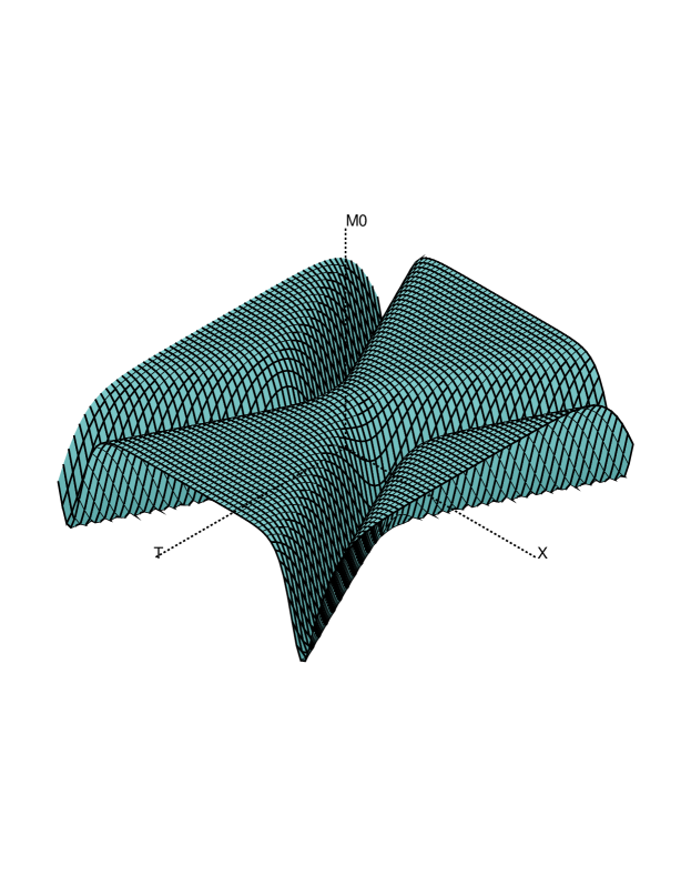
Figure 1: $M_{0}$ in soliton - soliton scattering

Figures (1)-(3) show $M_{0}\ ,\ M_{1}/i\ ,\ M_{2}/i$, as an example, for a specific case where $\theta=0.4\pi$ and the velocity $u=0.1$. From Eq.(7), the potential energy can be written by $V=2N\kappa M_{0}/\pi$ so that $M_{0}$ depicts the trajectory of soliton - soliton scattering in terms of minus the potential energy. $M_{0}$ shows that two solitons repulse each other at the origin. It is easy to read the $2\pi$-angle variation $\Delta|2\sqrt{\pi}\varphi|=2\pi$ across each bump from these figures which shows clearly that they describe the soliton - soliton scattering. Note that the internal direction given by the vector $\{\varphi_{i}\}$ changes after the collision. Under the spacetime inversion; $(T,X)\leftrightarrow(-T,-X)$, the solution in Eq.(94) possesses symmetry; $M_{0}\leftrightarrow M_{0},M_{i}\leftrightarrow-M_{i}\ ;\ i=1,2$. Thus, the internal directions of each solitons, specified by the components $\varphi_{i}$, become exchanged in the process of scattering. This is a characteristic of the scattering of nonabelian solitons. The minimum points of $M_{0}$ constitute a trajectory of the center of each solitons. At time $T=-T_{0}$ and $T=T_{0}$, two solitons are located at $\pm X_{0}$ which satisfies the relation,

$$\sinh{X_{0}^{2}}={2(\cos\theta-1)(\cosh^{2}T_{0}-1)\over 2\cosh^{2}T_{0}-1+\cos\theta}+{1\over u^{2}}\cosh^{2}T_{0}+{1\over 2}(1-\cos\theta)(1-{1\over u^{2}}).$$ (97)

Notice that at $T_{0}=0$, two solitons approach closest with

$$\sinh{X_{0}^{2}}={1\over u^{2}}{1+\cos\theta\over 2}+{1-\cos\theta\over 2}\ .$$ (98)

This shows that the repulsion between two solitons becomes maximum when two vectors $a_{i},\ \ b_{i}$ are aligned in the same direction which is precisely the abelian case where $\theta=0$. If $\theta=\pi$, $X_{0}$ takes a minimum value thereby maximizing the nonabelian effect. On the other hand, when $T_{0}$ becomes large, Eq.(97) can be approximated by

$$\sinh X_{0}^{2}\approx{1\over u^{2}}\cosh^{2}T_{0}\ .$$ (99)

The elapsing time for two solitons to bounce back to the separating distance $2X_{0}$ is given by $2T_{0}$. Thus, when $X_{0}$ becomes large, the elapsing time becomes independent of the angle $\theta$.

M=2, nonabelian breather

Now we consider the case (ii); $N^{\dagger}_{1}=-N_{2}$ in Eq.(75). We take $\mu_{1}=-\mu^{*}_{2}\equiv{i\over\sqrt{-\kappa}}\exp(i\alpha)$ and parameterize $N_{1}$ and $N_{2}$ by

$$N_{1} = i\exp(2\Delta)(c_{k}+id_{k})\sigma_{k}$$

$$N_{2} = i\exp(2\Delta^{*})(c_{k}-id_{k})\sigma_{k}$$ (100)

where $c_{i}c_{i}=d_{i}d_{i}=1$ and

$$2\Delta = 2\sqrt{-\kappa}[\exp(i\alpha)z-\exp(-i\alpha)\bar{z}]=2\sqrt{-\kappa}[(\cos\alpha)x+i(\sin\alpha)t]$$ (101)

$$\equiv K(x+ivt)\ \ ;\ \ K\equiv{2\sqrt{-\kappa}\over\sqrt{1+v^{2}}}\ ,\ v\equiv\tan\alpha\ .$$

A straightforward calculation shows that Eq.(62) holds for $N_{1},N_{2}$ given in Eq.(100). We could follow a similar procedure as in the case of the two soliton scattering and make use of the fact; $Z^{\dagger}_{12}=Z_{21},\ \ Z^{\dagger}_{11}=Z_{22}$ and $N^{2}_{1}$ is proportional to the identity matrix.

From Eqs.(66) and (100), we have,

$$Y^{-1}=(\det Y)^{-1}\pmatrix{(1+N_{1}N^{\dagger}_{1})[1+\exp(-2i\alpha)]^{-1}&ic_{i}d_{i}\exp(4\Delta^{*})-{1\over 2}\cr-ic_{i}d_{i}\exp(4\Delta)-{1\over 2}&(1+N^{\dagger}_{1}N_{1})[1+\exp(2i\alpha)]^{-1}}$$ (102)

where

$$\det Y={v^{2}\over 4}[1+4(c_{i}d_{i})^{2}e^{4Kx}]+(1+v^{2})e^{2Kx}+c_{i}d_{i}e^{2Kx}\sin(2Kvt).$$ (103)

Then, $g^{-1}_{1}g_{2}$ for the breather solution can be obtained from Eq.(67), or consistently from Eq.(68), which we write in the form;

$$g^{-1}_{1}g_{2} = (A+B^{i}_{+}\sigma_{i})(A+B^{i}_{-}\sigma_{i})^{-1}$$ (104)

$$\equiv M_{0}+M_{i}\sigma_{i}$$

where

$$A = {v^{2}\over 4}[1+4(c_{i}d_{i})^{2}e^{4Kx}]+(v^{2}-1)e^{2Kx}-c_{i}d_{i}e^{2Kx}\sin 2Kvt$$ (105)

$$B^{i}_{\pm} = \pm ic_{i}v(e^{Kx}\sin Kvt+2c_{k}d_{k}e^{3Kx}\cos Kvt)-2ive^{2Kx}\epsilon_{ijk}c_{j}d_{k}.$$ (106)

$$\pm id_{i}v(e^{Kx}\cos Kvt+2c_{k}d_{k}e^{3Kx}\sin Kvt)$$

and

$$M_{0} = 1-{2v^{2}\over(\det Y)^{2}}\biggl{[}e^{2Kx}\{1+4(c_{i}d_{i})^{2}e^{4Kx}\}(1+c_{i}d_{i}\sin 2Kvt)+4c_{i}d_{i}e^{4Kx}(c_{i}d_{i}+\sin 2Kvt)\biggr{]}$$

$$M_{i} = {1\over(\det Y)^{2}}\biggl{[}(e^{Kx}\sin Kvt+2c_{k}d_{k}e^{3Kx}\cos Kvt)\{2iAc_{i}v+4iv^{2}e^{2Kx}(d_{i}-c_{k}d_{k}c_{i})\}$$ (107)

$$+(e^{Kx}\cos Kvt+2c_{k}d_{k}e^{3Kx}\sin Kvt)\{2iAd_{i}v+4iv^{2}e^{2Kx}(c_{k}d_{k}d_{i}-c_{i})\}\biggr{]}.$$

In addition, a straightforward calculation shows that

$$g^{-1}_{1}\partial g_{1} = 2i\kappa\sum_{\alpha,\beta}(Z^{-1})_{\alpha\beta}$$ (108)

$$= -{2i\sqrt{-\kappa}\over\det Y}\biggl{[}ie^{i\alpha+2\Delta}(-{v\over 2}+ivc_{k}d_{k}e^{4\Delta^{*}})(c_{j}+id_{j})\sigma_{j}+c.c.\biggr{]}\ ,$$

which together with Eqs.(104)-(107) satisfies the matrix sine-Gordon equation (12).

For a pictorial description of a nonabelian breather, we choose without loss of generality $\{c_{i}\}=(1,0,0)\ ,\ \{d_{i}\}=(\cos\theta,\sin\theta,0)$. Then,

$$M_{0} = 1-{2v^{2}\over P_{+}^{2}}\biggl{[}e^{2Kx}(1+4\cos^{2}\theta e^{4Kx})(1+\cos\theta\sin 2Kvt)+4\cos\theta e^{4Kx}(\cos\theta+\sin 2Kvt)\biggr{]}$$

$$M_{1} = {2iv\over P_{+}^{2}}\biggl{[}(P_{-}e^{Kx}+2\cos^{2}\theta P_{-}e^{3Kx}-4v\cos\theta\sin^{2}\theta e^{5Kx})\sin Kvt$$

$$+(\cos\theta P_{-}e^{Kx}+2\cos\theta P_{-}e^{3Kx}-2v\sin^{2}\theta e^{3Kx})\cos Kvt\biggr{]}$$

$$M_{2} = {2iv\over P_{+}^{2}}\biggl{[}(\sin 2\theta P_{-}e^{3Kx}+2v\sin\theta e^{3Kx}+2v\cos\theta\sin 2\theta e^{5Kx})\sin Kvt$$

$$+(P_{-}\sin\theta e^{Kx}+v\sin 2\theta e^{3Kx}+2v\sin 2\theta e^{5Kx})\cos Kvt\biggr{]}$$

$$M_{3} = 0\ ,$$ (109)

where

$$P_{\pm}={v^{2}\over 4}[1+4\cos^{2}\theta e^{4Kx}]\pm(1\pm v^{2})e^{2Kx}\pm\cos\theta e^{2Kx}\sin(2Kvt).$$ (110)

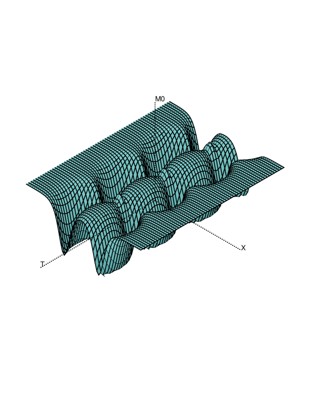
Figure 4: $M_{0}$ of nonabelian breather

Figures (4)-(6) show $M_{0}\ ,\ M_{1}/i\ ,\ M_{2}/i$ for a specific case where $\theta=\pi/6$ and $v=0.1$. The potential energy profile given in terms of $M_{0}$ shows clearly the breathing motion. The behavior of $\varphi_{i}$ in Eq.(96) along the $X$-direction in the figures of $M_{0},M_{1}$ and $M_{2}$ confirms that the breather solution is indeed a bound state of soliton and antisoliton. In addition, $M_{1}$ and $M_{2}$ shows that the internal direction of the breather also oscillates which is a characteristic of a nonabelian breather. Two particular values of $\theta$ are worth to address. If $\theta=0$, we may follow a similar procedure as in the 2-soliton case, and see that the nonabelian breather reduces to the well known sine-Gordon breather,

$$\varphi=\pm{2\over\sqrt{\pi}}\tan^{-1}{\sin(Kvt+{\pi\over 4})\over v\cosh(Kx+\mbox{ln}\sqrt{2})}\ .$$ (111)

For $\theta=\pi/2$, it is interesting to note that $M_{0}$ becomes independent of $t$ while $M_{1}$ and $M_{2}$ are not. This shows that the nonabelian breather at $\theta=\pi/2$ breathes only internally. That is, the internal direction oscillates while the potential energy remains static, i.e. externally it becomes completely breatheless.

4 Bäcklund Transformation

The Bäcklund transformation(BT) is a mapping between two solution surfaces of certain differential equations. For example, the sine-Gordon equation $\partial\bar{\partial}\phi=\sin\phi$ is invariant under the BT

$$\partial\tilde{\phi} = \partial\phi-2\delta\sin({\phi+\tilde{\phi}\over 2})$$

$$\bar{\partial}\tilde{\phi} = -\bar{\partial}\phi+{2\over\delta}\sin({\phi-\tilde{\phi}\over 2})$$ (112)

where $\delta$ is a nonzero real parameter. The integrability of Eq.(112) is the requirement that $\phi$ and $\tilde{\phi}$ are both solutions of the sine-Gordon equation. Thus the BT generates a new solution from a known one. Moreover, through the Bianchi’s permutability theorem, it leads to a nonlinear superposition of solutions which gives rise to a new solution by purely algebraic means. For example, if $\phi_{a},\phi_{b}$ are two solutions generated by the BT from a known solution $\phi_{g}$ with Bäcklund parameters $\delta_{1},\delta_{2}$ respectively, then the Bianchi’s permutability theorem[9] gives a new solution $\phi_{h}$ by

$$\phi_{h}=\phi_{g}+4\mbox{tan}^{-1}({\delta_{1}+\delta_{2}\over\delta_{1}-\delta_{2}}\tan{\phi_{a}-\phi_{b}\over 4})$$ (113)

In this section, we show that all these properties generalize to the matrix sine-Gordon theory. Recall that the linear equation for the matrix sine-Gordon equation is

$$[\partial+g^{-1}\partial g-\lambda T]\Psi_{g}=0\ ;\ [\bar{\partial}+{1\over\lambda}g^{-1}\bar{T}g]\Psi_{g}=0$$ (114)

where $T,\bar{T}$ are as in Eq.(20). The BT between two solutions $g$ and $f$ of the matrix sine-Gordon equation may be defined in terms of $\Psi$,

$$\Psi_{f}={\lambda\over\lambda+i\delta}(1+{\delta\over\lambda}f^{-1}\bar{T}g)\Psi_{g}$$ (115)

where $\delta$ is a real Bäcklund parameter. $\Psi_{f}$ and $\Psi_{g}$ both satisfy the linear equation with respect to $f$ and $g$. On the other hand, if Eq.(115) is combined with the linear equation (114) to elliminate $\Psi$, then we have an equivalent expression for the BT in terms of $f$ and $g$,

$$f^{-1}\partial f-g^{-1}\partial g+\delta[g^{-1}\bar{T}f\ ,\ T]=0$$ (116)

and

$$gf^{-1}\bar{T}-\bar{T}gf^{-1}-\delta\bar{\partial}gg^{-1}\bar{T}+\delta\bar{T}\bar{\partial}ff^{-1}=0$$ (117)

Also, the unitarity condition, $\Psi(\lambda^{*})\Psi^{\dagger}(\lambda)=1$, requires that

$$f^{-1}\bar{T}g-g^{-1}\bar{T}f=0.$$ (118)

Eqs. (115) - (118) consitute the BT for the matrix sine-Gordon equation. With $g\ ,\ T\ ,\ \bar{T}$ as in Eqs.(20) and (21), Eqs.(116) and (117) in block components are

$$f^{-1}_{1}\partial f_{1}-g^{-1}_{1}\partial g_{1}+\kappa\delta(g^{-1}_{2}f_{1}-g^{-1}_{1}f_{2}) = 0$$

$$f^{-1}_{2}\partial f_{2}-g^{-1}_{2}\partial g_{2}-\kappa\delta(g^{-1}_{2}f_{1}-g^{-1}_{1}f_{2}) = 0$$ (119)

and

$$\bar{\partial}f_{1}f^{-1}_{1}-\bar{\partial}g_{2}g^{-1}_{2}+{1\over\delta}(g_{2}f^{-1}_{2}-g_{1}f^{-1}_{1}) = 0$$

$$\bar{\partial}f_{2}f^{-1}_{2}-\bar{\partial}g_{1}g^{-1}_{1}-{1\over\delta}(g_{2}f^{-1}_{2}-g_{1}f^{-1}_{1}) = 0,$$ (120)

while Eq.(118) becomes

$$f^{-1}_{1}g_{2}=g^{-1}_{1}f_{2}.$$ (121)

Note that Eqs.(119) and (120) are consistent with the constraint equation (13). We now show that the matrix sine-Gordon theory admit also a nonlinear superposition rule of solutions which generates a new solution by purely algebraic means. This is given by the permutability of the Bianchi diagram. Let $a$ and $b$ are solutions of the matrix sine-Gordon equation generated by the BT from a known solution $g$ with the Bäcklund parameters $\delta_{1}$ and $\delta_{2}$ respectively. Further, let $h$ and $h^{{}^{\prime}}$ denote solutions obtained by applications of the BT with parameter $\delta_{2}$ to $a$ and with parameter $\delta_{1}$ to $b$. Then, the permutability of the Bianchi diagram requires $h=h^{{}^{\prime}}$. In terms of the BT in Eq.(115), this means that

$$\Psi_{h} = {\lambda\over\lambda+i\delta_{2}}\ {\lambda\over\lambda+i\delta_{1}}(1+{\delta_{2}\over\lambda}h^{-1}\bar{T}a)(1+{\delta_{1}\over\lambda}a^{-1}\bar{T}g)\Psi_{g}$$ (122)

$$= {\lambda\over\lambda+i\delta_{1}}\ {\lambda\over\lambda+i\delta_{2}}(1+{\delta_{1}\over\lambda}h^{-1}\bar{T}b)(1+{\delta_{2}\over\lambda}b^{-1}\bar{T}g)\Psi_{g}$$

or

$$(1+{\delta_{2}\over\lambda}h^{-1}\bar{T}a)(1+{\delta_{1}\over\lambda}a^{-1}\bar{T}g)=(1+{\delta_{1}\over\lambda}h^{-1}\bar{T}b)(1+{\delta_{2}\over\lambda}b^{-1}\bar{T}g)$$ (123)

which, when solved for $h$ using the relation $\bar{T}ga^{-1}\bar{T}^{-1}=ag^{-1}$, gives

$$h=g(\delta_{1}b^{-1}-\delta_{2}a^{-1})(\delta_{1}a^{-1}-\delta_{2}b^{-1})^{-1}.$$ (124)

or, in terms of $h_{1}$ and $h_{2}$,

$$h_{1} = g_{1}(\delta_{1}b_{1}^{-1}-\delta_{2}a_{1}^{-1})(\delta_{1}a_{1}^{-1}-\delta_{2}b_{1}^{-1})^{-1}$$

$$h_{2} = g_{2}(\delta_{1}b_{2}^{-1}-\delta_{2}a_{2}^{-1})(\delta_{1}a_{2}^{-1}-\delta_{2}b_{2}^{-1})^{-1}\ .$$ (125)

It is easy to check that $h$ is unitary if $a,b$ are unitary. This is the nonlinear superposition rule of the matrix sine-Gordon equation which allows one to generate a new solution from a known one by purely algebraic means. In the abelian limit, we may take $h=\exp{i\phi_{h}\sigma_{3}/2}\ ,\ b=\exp{i\phi_{b}\sigma_{3}/2}\ ,\ a=\exp{i\phi_{a}\sigma_{3}/2}\ ,\ g=\exp{i\phi_{g}\sigma_{3}/2}$, then Eq.(124) reduces precisely to the nonlinear superposition rule of the sine-Gordon equation in Eq.(113).

Finally, we obtain one and two soliton solutions of the theory using the BT. We take the trivial solution to be a vacuum given by $f_{1}=f_{2}=f$ for a constant $SU(2)$ matrix $f$. Then, the 1-soliton solution in terms of $g_{1}$, $g_{2}$ is obtained through the BT in Eqs.(119) and (120) which, after redefining $g_{1},g_{2}$ by $g_{1}f^{-1}\rightarrow g_{1},\ \ g_{2}f^{-1}\rightarrow g_{2}$, becomes

$$g^{-1}_{1}\partial g_{1}-\kappa\delta(g^{-1}_{2}-g^{-1}_{1}) = 0$$

$$\bar{\partial}g_{1}g^{-1}_{1}+{1\over\delta}(g_{2}-g_{1}) = 0.$$ (126)

and the same equation with $g_{1}$ and $g_{2}$ interchanged. If we use the parametrization for $g_{1}$ and $g_{2}$,

$$g_{1}=\pmatrix{u&i\sqrt{1-uu^{*}}e^{i\phi}\cr i\sqrt{1-uu^{*}}e^{-i\phi}&u^{*}}\ ,\ g_{2}=\pmatrix{v&i\sqrt{1-vv^{*}}e^{i\theta}\cr i\sqrt{1-vv^{*}}e^{-i\theta}&v^{*}}\ ,$$ (127)

Eq.(126) resolves into the component equations;

$$u^{*}\partial u-u\partial u^{*}-2i(1-uu^{*})\partial\phi-2\kappa\delta(v^{*}-u^{*}) = 0$$

$$\partial u-\kappa\delta(e^{i(\phi-\theta)}\sqrt{1-uu^{*}}\sqrt{1-vv^{*}}-1+uv^{*}) = 0$$

$$u\bar{\partial}u^{*}-u^{*}\bar{\partial}u-2i(1-uu^{*})\bar{\partial}\phi+2{1\over\delta}(u-v) = 0$$

$$\bar{\partial}u-{1\over\delta}(e^{i(\theta-\phi)}\sqrt{1-uu^{*}}\sqrt{1-vv^{*}}-1+uv^{*}) = 0$$ (128)

and the same equation with the interchange; $u\leftrightarrow v,\phi\leftrightarrow\theta$. In addition, the traceless conditon of Eq.(126) requires that $u+u^{*}=v+v^{*}$. The unitarity condition, Eq.(121), in this case requires that $u=v^{*}$ and $\phi=\theta+\pi$. Then, equations for $u$ and $u^{*}$ become

$$({1\over\kappa\delta}\partial-\delta\bar{\partial})u = 0$$

$$({1\over\kappa\delta}\partial+\delta\bar{\partial})u = -4+2uu^{*}+2u^{2}$$ (129)

and the same equation with $u$ and $u^{*}$ interchanged. This equation can be readily integrated to give $u+u^{*}=2\tanh(2\Delta+\eta)\ ;\ \Delta=-\kappa\delta z-\bar{z}/\delta$ and

$$u=\tanh(2\Delta+\eta)+ic{1\over\cosh(2\Delta+\eta)},$$ (130)

where c is an arbitrary constant. In addition, when the solution $u$ is used, Eq.(128) can be solved for $\phi$ such that $\phi$ is a constant. In terms of $g_{1}$ and $g_{2}$, this means that

$$g_{1} = g_{2}^{-1}={1-N\over 1+N}$$

$$N = ie^{2\Delta+\eta}a_{k}\sigma_{k}\ ,\ V\equiv(1+\kappa\delta^{2})/(1-\kappa\delta^{2})$$

$$\Delta = -\kappa\delta z-{1\over\delta}\bar{z}=\pm{\sqrt{-\kappa}\over\sqrt{1-V^{2}}}(x-Vt)$$ (131)

where $\eta,a_{i}$ are arbitrary constants coming from $c$ and $\phi$ with normalization $a_{i}a_{i}=1$. This agrees precisely with the 1-soliton solution in Sec.3.

In order to obtain two soliton solutions, we may apply the nonlinear superposition rule to a couple of one soliton solutions obtained by the BT with parameters $\delta_{1}$ and $\delta_{2}$ such that

$$a_{1}=a_{2}^{-1}={1-N_{1}\over 1+N_{1}},\ ;\ b_{1}=b_{2}^{-1}={1-N_{2}\over 1+N_{2}}$$ (132)

where $N_{1},\ N_{2}$ are given in Eq.(131) with repective parameters $\delta_{1},\eta_{1}$ and $\delta_{2},\eta_{2}$. Then, from Eq.(125) we obtain the 2-soliton solution,

$$h^{-1}_{1} = \left(\delta_{1}{1+N_{1}\over 1-N_{1}}-\delta_{2}{1+N_{2}\over 1-N_{2}}\right)\left(\delta_{1}{1+N_{2}\over 1-N_{2}}-\delta_{2}{1+N_{1}\over 1-N_{1}}\right)^{-1}$$

$$h^{-1}_{2} = \left(\delta_{1}{1-N_{1}\over 1+N_{1}}-\delta_{2}{1-N_{2}\over 1+N_{2}}\right)\left(\delta_{1}{1-N_{2}\over 1+N_{2}}-\delta_{2}{1-N_{1}\over 1+N_{1}}\right)^{-1}\ .$$ (133)

It is now a straightforward but amusing exercise to check that $h_{1}^{-1}$ is equal to $(A+B^{k}_{+}\sigma_{k})/\det Y$ of Eqs.(79) and (80) while $h^{-1}_{2}$ is equal to $(A+B^{k}_{-}\sigma_{k})/\det Y$.

5 Discussion

Throughout this Paper, we have analyzed various classical properties of the matrix sine-Gordon theory for the coupling constant $\kappa<0$. For $\kappa>0$, the vacuum structure changes, i.e. degenerate vacuua occur at $\phi=(2n+1)\pi$ for integer $n$ so that $g^{-1}_{1}g_{2}=-1$, or for $g_{1}=-g_{2}=f$ for arbitrary $f$. This reflects the symmetry of the matrix sine-Gordon theory under the exchange;

$$g_{1}\leftrightarrow g_{1}\ ,\ g_{2}\leftrightarrow-g_{2}\ ,\ \kappa\leftrightarrow-\kappa\ .$$ (134)

Thus, the matrix sine-Gordon theory with $\kappa>0$ is identical with the $\kappa<0$ case except the sign change of $g_{2}$. This type of symmetry arises due to a specific choice of the potential term and can be generalized to other types of nonabelian sine-Gordon theory considered in [4] [5] [6]. In the abelian sine-Gordon case, the potential is given by $\kappa\cos{\phi}$ and the symmetry becomes the well-known one;

$$\phi\leftrightarrow\phi+\pi\ ,\ \kappa\leftrightarrow-\kappa\ .$$ (135)

In finding exact solutions, solitons and breathers, we have assumed asymptotic boundary conditions $g_{1},g_{2}\rightarrow 1$ as $x\rightarrow\pm\infty$. However, this boundary condition may be relaxed to accomodate other types of solutions. For example, if we impose a periodic boundary condition, i.e. choose the underlying manifold to be a torus, we can not take a nonlocal gauge where $A=\bar{A}=0$ except for the trivial holonomy sector of the flat connection $A$ and $\bar{A}$. Nontrivial sectors could lead to generalizations of solitons and breathers of the matrix sine-Gordon theory characterized by the nontrivial holonomy. Another important classical aspect of the matrix sine-Gordon theory which we have not considered is the hamiltonian struture of the theory. As in the case of solitons, we expect a nontrivial generalization of the hamiltonian structure of the sine-Gordon theory, especially a nonabelian generalzation of the R-matrix.

The quantum matrix sine-Gordon theory is equally important and provides a nontrivial generalization of the quantum abelian sine-Gordon theory. Moreover, it is a natural quantum field theory framework for the Zamolodchikov’s integrable $\Phi_{(2,1)}$ perturbation of Ising model. In the parafermion case, the S-matrix obtained by Zamolodchikov using the operator algebra has been explained nicely in terms of the complex sine-Gordon theory[17]. Since the matrix sine-Gordon theory carries essentially the same structure as the complex sine-Gordon theory, one expect that a similar analysis is possible for this case using a semiclassical WKB approximation. Work in this direction is in progress and will appear elsewhere.

ACKNOWLEDGEMENT We would like to thank T.Hollowood for discussion. This work was supported in part by Research Fund of Kyunghee University, by the program of Basic Science Research, Ministry of Education BSRI-95, and by Korea Science and Engineering Foundation through CTP/SNU and the Korea-Japan Cooperative Science Program.

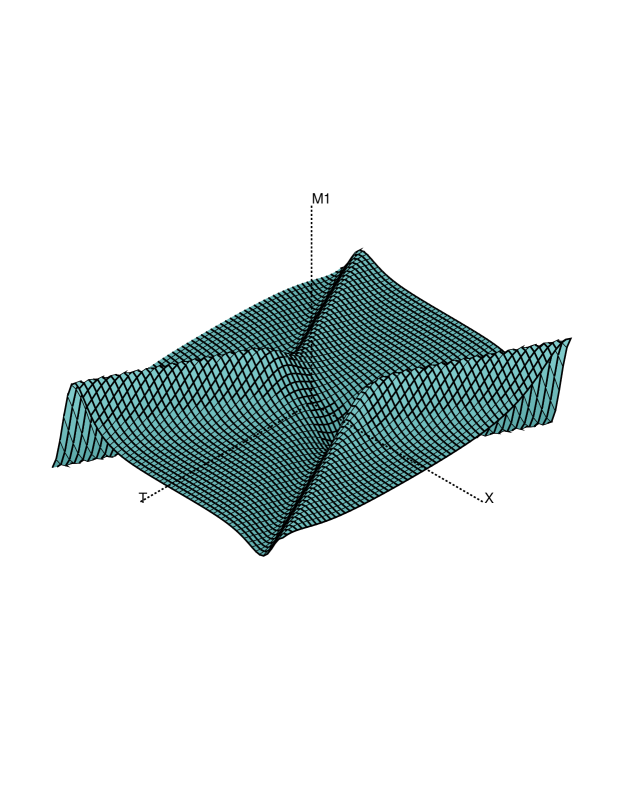
Figure 2: $M_{1}$ in soliton - soliton scattering

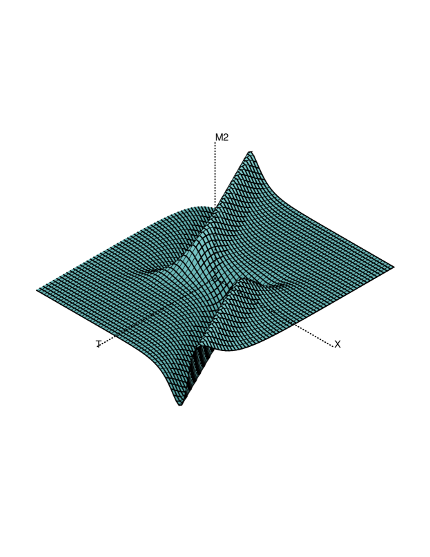
Figure 3: $M_{2}$ in soliton - soliton scattering

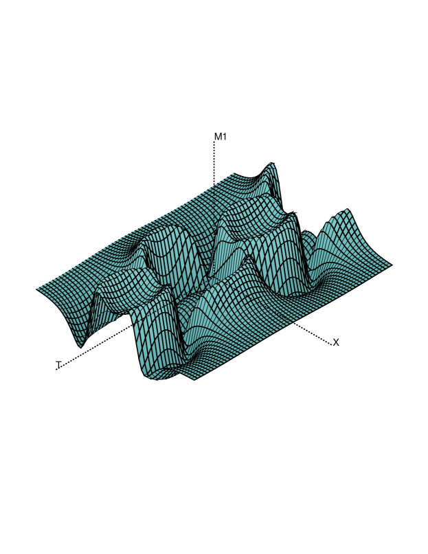
Figure 5: $M_{1}$ of nonabelian breather

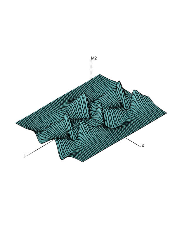
Figure 6: $M_{2}$ of nonabelian breather