USITP-95-06, UUITP-4/95

April 1995

The Moduli Space and Monodromies of
N=2 Supersymmetric $SO(2r+1)$ Yang-Mills Theory
Ulf H. Danielsson
Institutionen för teoretisk fysik

Box 803
S-751 08 Uppsala
Sweden
Bo Sundborg
Institute of Theoretical Physics
Fysikum
Box 6730
S-113 85 Stockholm
Sweden

We write down the weak-coupling limit of N=2 supersymmetric Yang-Mills theory with arbitrary gauge group $G$. We find the weak-coupling monodromies represented in terms of $Sp(2r,{\mathbbm{Z}})$ matrices depending on paths closed up to Weyl transformations in the Cartan space of complex dimension r, the rank of the group. There is a one to one relation between Weyl orbits of these paths and elements of a generalized braid group defined from $G$. We check that these weak-coupling monodromies behave correctly in limits of the moduli space corresponding to restrictions to subgroups. In the case of $SO(2r+1)$ we write down the complex curve representing the solution of the theory. We show that the curve has the correct monodromies.

1 Introduction

After the initial solution of $N=2$ SUSY Yang-Mills theory for $SU(2)$, [1], the extension to $SU(N_{c})$ has been studied in several papers, [2-4]. In this paper we will work out the details of yet another example: $SO(2r+1)$.

We should point out that the case of $SO(N_{c})$ has recently been studied in [5] for $N=1$ with matter in the vector representation. With one such matter field, the number of complex dimensions of the moduli space will always be one. In $N=1$ language, our case corresponds to matter in the adjoint representation. In that case, the number of complex dimensions will be $r$, the rank of the group.

The main result of the paper will be a proposal for a complex curve that will describe the moduli-space of $SO(2r+1)$. We will perform several tests to show that the curve has the correct properties. Among other things, we will recover the known vacuum structure for a $N=1$ theory. In addition, we give a uniform description of the weak coupling monodromies for all simple groups.

In $N=1$ super-space the Lagrangian is given by

$${1\over 4\pi}Im\left(\int d^{4}\theta{\partial{\cal F}(\Phi)\over\partial\Phi}\bar{\Phi}+\int d^{2}\theta{1\over 2}{\partial^{2}{\cal F}(\Phi)\over\partial\Phi^{2}}W^{2}\right),$$ (1)

where $W=(A,\lambda)$ is the a gauge field multiplet and $\Phi=(\phi,\psi)$ is a chiral multiplet, both taking values in the adjoint representation. The field $\phi$ is given a vacuum expectation-value according to

$$\phi=\sum_{i=1}^{r}b_{i}H_{i},$$ (2)

where $r$ is the rank of the group. $H_{i}$ are elements of the Cartan sub-algebra, and we have normalized so that $Tr(H_{i}H_{j})=\delta_{ij}$.

At a generic $b$ the gauge-group is broken down to $U(1)^{r}$ and each $W$-boson, one for each root $\alpha$, acquires a $(mass)^{2}$ proportional to $(\mbox{\boldmath$b$}\cdot\mbox{\boldmath$\alpha$})^{2}$. Restoration of symmetry (classically) is obtained when $b$ is orthogonal to a root. At such a point the $W$-boson corresponding to that root becomes massless.

The matrix of effective couplings, $\tau^{ij}$, is given by a one-loop expression

$$\tau^{ij}\sim{\partial^{2}\over\partial b_{i}\partial b_{j}}{\cal F}(\mbox{\boldmath$b$})\sim{i\over 2\pi}\sum_{\mbox{\boldmath$\alpha$}}\alpha^{i}\alpha^{j}\log{(\mbox{\boldmath$b$}\cdot\mbox{\boldmath$\alpha$})^{2}\over\Lambda^{2}}.$$ (3)

The sum is over all roots $\alpha$ of the algebra. Under a $U(1)_{R}$ transformation $\theta\rightarrow e^{i\omega}\theta$ the field $\phi$ has charge two and hence

$$\tau^{ij}\rightarrow\tau^{ij}-{2\omega\over\pi}\sum_{\mbox{\boldmath$\alpha$}}\alpha^{i}\alpha^{j}=\tau^{ij}-{2\omega C_{2}\over\pi}\delta^{ij},$$ (4)

where $C_{2}$ is the eigenvalue of the quadratic Casimir in the adjoint representation [6]. From this it follows that the second term in (1), i.e.

$$I={1\over 8\pi}Im\left(\int\tau^{ij}\left(F_{i}F_{j}+iF_{i}^{*}F_{j}\right)\right),$$ (5)

transforms as

$$I\rightarrow I-{\omega C_{2}\over 4\pi^{2}}\int F^{*}F=I-4\omega C_{2}n$$ (6)

where $n$ is the instanton number. This is consistent with the presence of the ABJ anomaly in the $U(1)_{R}$ current. The $U(1)_{R}$ symmetry is hence broken down to ${\mathbbm{Z}}_{4C_{2}}$ of which a ${\mathbbm{Z}}_{2C_{2}}$ acts on $\phi$ or $b$.

We also need the pre-potential ${\cal F}$ in the semi-classical limit. For a general group it is obtained by integrating the effective coupling (4) twice.

$${\cal F}\sim{i\over 4\pi}\sum_{\mbox{\boldmath$\alpha$}}(\Psi\cdot\mbox{\boldmath$\alpha$})^{2}\log{(\Psi\cdot\mbox{\boldmath$\alpha$})^{2}\over\Lambda^{2}},$$ (7)

where $\Psi$ is the $N=2$ superfield containing $W$ and $\Phi$.

2 Semi-classical monodromies

When considering the action of $Sp(2r,{\mathbbm{Z}})$ monodromy transformations on the scalar vevs we use the variables $a_{i}$ (defined later in eq. (25)) rather than the $b_{i}$. In the semi-classical limit they agree and can be used interchangeably, but in general they should be distinguished.

The prepotential ${\cal F}$ is invariant under the discrete Weyl subgroup of gauge transformations, simply because the sum in eq. (7) is over the set of all roots, which is itself invariant. However, the logarithms imply that paths starting at a point $a$ and ending at one of its Weyl images $w\mbox{\boldmath$a$}$ give rise to shifts of ${\cal F}$ when the path encircles some singular hyperplanes $\mbox{\boldmath$a$}\cdot\mbox{\boldmath$\alpha$}=0$. These planes are precisely the walls of the Weyl chambers in the complexified Cartan subalgebra. We fix the branch cuts of the logarithms in eq. (7) to lie along the negative real axis. Monodromy shifts can then be calculated by keeping track of how the path encircles the reflection hyperplanes in passing from Weyl chamber $C$ to Weyl chamber $wC$. Each time a branch cut is passed a shift of ${\cal F}$ is given by the change in the imaginary part of the logarithm, compared to the original expression.

For $SU(r+1)$ the Weyl group is the permutation group on $r+1$ elements and it is generated by the $r$ reflections $s_{k}$ in the walls of the fundamental domain $D$ given by

$$Re(\mbox{\boldmath$a$}\cdot\mbox{\boldmath$\alpha$}_{k})>0.$$ (8)

Here $(\mbox{\boldmath$\alpha$}_{k})_{k=1}^{r}$ are simple roots of $SU(r+1)$. Keeping track of paths means to keep track of how many units of $\pi$ the phase of $\mbox{\boldmath$a$}\cdot\mbox{\boldmath$\alpha$}$ changes with as its zero is encircled. In terms of permutations one may think of permuting complex numbers and keeping track of how they move around each other in the complex plane. Composition of paths by joining an endpoint to an initial point then gives rise to a larger group than the Weyl group, the braid group on $r+1$ elements.

For other simple groups there is an appropriate generalization of the ordinary braid group called the Brieskorn braid group, defined solely in terms of the Weyl group [7] (or equivalently the Dynkin diagram of the group). To each vertex of a Dynkin diagram corresponds a simple root $\mbox{\boldmath$\alpha$}_{k}$, a Weyl reflection $s_{k}$ and a simple braid $t_{k}$. The braid and Weyl groups are generated by these sets of $r$ elements and the defining relations

$$\underbrace{t_{m}t_{n}t_{m}\ldots}_{l_{mn}}\underbrace{\ldots t_{n}^{-1}t_{m}^{-1}t_{n}^{-1}}_{l_{mn}} = 1$$ (9)

$$\underbrace{s_{m}s_{n}s_{m}\ldots}_{l_{mn}}\underbrace{\ldots s_{n}^{-1}s_{m}^{-1}s_{n}^{-1}}_{l_{mn}} = 1$$ (10)

$$s_{m}^{2} = 1$$ (11)

where $l_{mn}$ is $3,4$ or $6$ for $1,2$ or $3$ links, respectively, joining vertex $m$ and $n$ of the Dynkin diagram. The braids of the braid group are in a one to one correspondence with the equivalence classes of paths that each pick up different logarithmic contributions in moving from a base point to one of its Weyl images.

So far we have only discussed how to multiply braids, but we are also interested in how they act on the physical fields, $a_{i}$ and their duals

$$a_{D}^{i}\equiv{\partial{\cal F}\over\partial a_{i}}\sim{i\over 2\pi}\sum_{\mbox{\boldmath$\alpha$}}(\mbox{\boldmath$a$}\cdot\mbox{\boldmath$\alpha$})\alpha^{i}(1+\log{(\mbox{\boldmath$a$}\cdot\mbox{\boldmath$\alpha$})^{2}\over\Lambda^{2}}).$$ (12)

The non-logarithmic term is a Weyl invariant matrix multiplying $a_{i}$, so it has to be proportional to the Cartan metric. We choose an orthonormal basis of Lie algebra to simplify the notation. (Note that the bases of the $SU(r+1)$ Cartan algebras in [2] and [3] are non-orthonormal). Then the semi-classical monodromies from (12) take the general form

$$\pmatrix{\mbox{\boldmath$a$}_{D}\cr\mbox{\boldmath$a$}\cr}\to M\pmatrix{\mbox{\boldmath$a$}_{D}\cr\mbox{\boldmath$a$}\cr}\equiv\pmatrix{w&m\cr 0&w\cr}\pmatrix{\mbox{\boldmath$a$}_{D}\cr\mbox{\boldmath$a$}\cr}$$ (13)

where $m$ contains the non-trivial contribution to the monodromy from the logarithms. The discussion of the Brieskorn braid group applies to the evaluation of $m$. In particular, it is enough to calculate the monodromy matrices for $r$ generating braids, since the rest of the monodromies should represent the braid group. However, some care is needed in order to multiply the monodromies, since the minimum number of singularities which a point has to encircle in going from $a$ to its Weyl image $w\mbox{\boldmath$a$}$ depends on which Weyl chamber $a$ belongs to.

Let us try to generate all semi-classical monodromies from $r$ simple monodromies which only receive contributions from a single logarithm of (12). This can be achieved by identifying the simple monodromies with the $r$ transformations resulting from paths winding (in the positive sense) around the $r$ walls of the Weyl chamber containing $a$. For example, $a$ can belong to the fundamental domain given by eq. (8). Then there is a Weyl reflection $s_{k}$ about each wall $\mbox{\boldmath$a$}\cdot\mbox{\boldmath$\alpha$}_{k}=0$, and in the corresponding monodromy path only the logarithm with argument $(\mbox{\boldmath$a$}\cdot\mbox{\boldmath$\alpha$}_{k})^{2}$ encounters a branch cut. At the branch cut an additional phase of $2\pi$ is generated, and a non-trivial monodromy matrix $M_{k}$ can be read off:

$$M_{k}\equiv\pmatrix{{\mathbbm{1}}-2{\mbox{\boldmath$\alpha$}_{k}\otimes\mbox{\boldmath$\alpha$}_{k}\over\mbox{\boldmath$\alpha$}_{k}^{2}}&-\mbox{\boldmath$\alpha$}_{k}\otimes\mbox{\boldmath$\alpha$}_{k}\cr 0&{\mathbbm{1}}-2{\mbox{\boldmath$\alpha$}_{k}\otimes\mbox{\boldmath$\alpha$}_{k}\over\mbox{\boldmath$\alpha$}_{k}^{2}}\cr}.$$ (14)

Even though the form of these simple monodromies is determined by their action on $a$ in the fundamental domain $D$, their domain of definition can be extended by linearity to the whole set of regular Weyl orbits (the Cartan subalgebra minus the Weyl chamber walls). Then it is possible to define the products of simple monodromies simply as matrix multiplication. However, in Weyl chambers $C$ other than $D$ the $M_{k}$ represent paths through the images of the walls of $D$ under the (unique) Weyl transformation $w$ mapping $D$ to $C=wD$, rather than paths through the walls of the fundamental domain itself.

Then the monodromies $M_{k}$ should generate a representation of the Brieskorn braid group. Indeed, we have checked, for all simple groups, that they satisfy

$$\underbrace{M_{m}M_{n}M_{m}\ldots}_{l_{mn}}\underbrace{\ldots M_{n}^{-1}M_{m}^{-1}M_{n}^{-1}}_{l_{mn}}=1,$$ (15)

which are the images of the defining relations (9) of the braid group.

3 The complex curve for $SO(2r+1)$

3.1 Constructing the curve

We will now construct a complex curve appropriate for the $SO(2r+1)$ case. It must satisfy two requirements. First it must be symmetric under the Weyl group. Second, it should be symmetric under the $U(1)_{R}$ acting on $\phi$ in the (unphysical) limit of vanishing $\Lambda$, but due to instantons this symmetry should be broken to ${\mathbbm{Z}}_{2C_{2}}$ for general $\Lambda$. For $SO(2r+1)$ we have that $C_{2}=2r-1$. The Weyl group of $SO(2r+1)$ acts as the group of all permutations and sign changes of the $r$ numbers $b_{i}$ of eq. (2). The $b_{i}$ can be used to parametrize the curve and have $U(1)_{R}$ charge two. With this information it is natural to try the curve

$$y^{2}=((x^{2}-b_{1}^{2})...(x^{2}-b_{r}^{2}))^{2}-\Lambda^{4r-2}x^{2}.$$ (16)

If we assign $U(1)_{R}$ charges $2$ to $x$ and $4r$ to $y$, we see that the $U(1)_{R}$ symmetry of the curve is broken to ${\mathbbm{Z}}_{4r-2}$ by the term depending on $\Lambda$. In fact, since the inversion ${\mathbbm{Z}}_{2}$ of the Weyl-group (as in the case of $SU(2)$) coincides with the ${\mathbbm{Z}}_{2}$ inside ${\mathbbm{Z}}_{4r-2}$, there will only be a ${\mathbbm{Z}}_{2r-1}$ acting on the moduli-space. Furthermore, the curve will depend on $\phi$ only through Weyl invariant polynomials, for which the Casimirs $Tr(\phi^{2k})$ provide a basis.

To verify that this indeed is the correct curve, it is necessary to check the semi-classical monodromies of the curve.

3.2 Partial symmetry breaking and factorization of the curve

The monodromies can be obtained from the curve by introducing $r$ pairs of homology cycles $(\gamma_{D}^{i},\gamma_{i})$ on the curve, one for each $b_{i}$, and then following how they transform as the parameters of the curve are varied to a Weyl equivalent point. The semi-classical limits consist in taking some

$$|b_{i}|>>\Lambda.$$ (17)

The fields $a_{i}$ will be defined in terms of the curve so as to ensure that $b_{i}\to a_{i}$ smoothly in these limits. Then a transformation of the homology cycles $(\gamma_{D}^{i},\gamma_{i})$ can be interpreted as a monodromy transformation on the $(a_{D}^{i},a_{i})^{t}$ vectors. By taking only a subset of the $b_{i}$ to be large, the symmetry is only partially broken. Hence, it should be possible to read off the curves corresponding to subgroups of the full unbroken gauge symmetry by taking appropriate limits of the $b_{i}$. For the $SO(2r+1)$ curves (16) it works as follows.

By deleting a vertex from the Dynkin diagram of a group, one gets subgroups of rank $r-1$. These subgroups are seen from the curve by taking the limit $\mbox{\boldmath$b$}\cdot\mbox{\boldmath$\alpha$}_{k}\to\infty$ while keeping the scalar products with the other simple roots fixed, i.e. by moving $a$ far away from the reflection hyperplane of the root $\mbox{\boldmath$\alpha$}_{k}$ corresponding to the deleted vertex. For $SO(2r+1)$ a canonical choice of simple roots is

$$\mbox{\boldmath$\alpha$}_{k} = \hat{e}_{k}-\hat{e}_{k+1},k=1,\ldots,r-1$$ (18)

$$\mbox{\boldmath$\alpha$}_{r} = \hat{e}_{r}$$ (19)

in terms of an ON basis. Deleting $\mbox{\boldmath$\alpha$}_{1}$ produces simple roots of $SO(2r-1)$, deleting $\mbox{\boldmath$\alpha$}_{r}$ gives simple roots of $SU(r)$ and removing one of the other roots $\mbox{\boldmath$\alpha$}_{k}$ yields $SU(k)\times SO(2r-2k+1)$. The prepotential ${\cal F}$ respects this sub-group structure and so should the curve (16). Let us check the case when a vertex inside the Dynkin diagram is deleted.

Taking the limit $\mbox{\boldmath$b$}\cdot\mbox{\boldmath$\alpha$}_{k}\to\infty$ and defining new parameters

$$kB = b_{1}+\ldots+b_{k}$$ (20)

$$\hat{b}_{i} = b_{i}-B,i=1,\ldots,k$$ (21)

the curve takes the form

$$y^{2} = (x-\hat{b}_{1}-B)^{2}\ldots(x-\hat{b}_{k}-B)^{2}(x+\hat{b}_{1}+B)^{2}\ldots(x+\hat{b}_{k}+B)^{2}$$ (22)

$$\times(x^{2}-b_{k+1}^{2})^{2}\ldots(x^{2}-b_{r}^{2})^{2}-\Lambda^{4r-2}x^{2}.$$

We see that the product on the right hand side of the equation factorizes into three groups of factors. In the limit $B\to\infty$, which is precisely the limit we are considering, the zeroes inside each group are at finite distances from each other, while distances between zeroes in different groups diverge. For fixed $x$ the curve then approaches the form

$$y^{2}=(x^{2}-b_{k+1}^{2})^{2}\ldots(x^{2}-b_{r}^{2})^{2}-\Lambda^{4r-4k-2}x^{2}$$ (23)

after a rescaling of $y$ and renormalization group matching of $\Lambda_{SO(2r-2k+1)}$ to $\Lambda_{SO(2r+1)}$. We recognize the expression for an $SO(2r-2k+1)$ curve!

If instead the regions around $x=\pm B$ are studied, one obtains in a similar way

$$y^{2}=((x\mp\hat{b}_{1})\ldots(x\mp\hat{b}_{k}))^{2}-\Lambda^{2k}$$ (24)

after also shifting $x$. These curves are precisely the $SU(k)$ curves of Argyres and Faraggi [2] and of Klemm, Lerche, Yankielowicz and Theisen [3]. Even though two $SU(k)$ curves appear in this factorization they only represent one group factor, since they are exact mirror images of each other. For removal of vertices at the ends of the Dynkin diagram, $k=1$ or $k=r$, almost identical arguments give the expected symmetry breaking.

3.3 Checking the monodromies for $SO(5)$

Let us consider the $SO(5)$ case in some detail! The semi-classical monodromies can be checked by acting with the braid group on the $b$’s and keeping track of the cycles. We choose a basis of cycles as in figure 1.

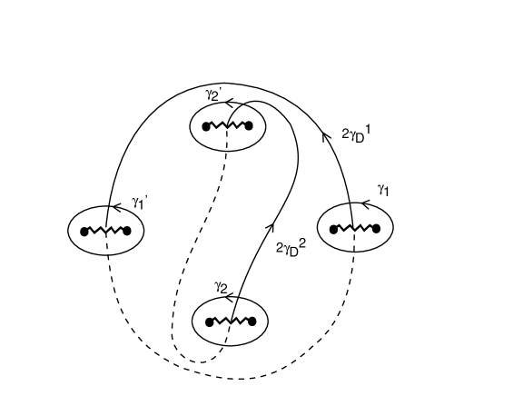
Figure 1: Cycles for the SO(5) curve.

The fields transforming simply under $Sp(2r,{\mathbbm{Z}})$ duality are $a_{i}$ and $a_{D}^{i}$, and they are given by the following integrals over cycles

$$a_{i}=\oint_{\gamma_{i}}\lambda\;\;\;\;\mbox{and}\;\;\;\;a_{D}^{i}=\oint_{\gamma_{D}^{i}}\lambda.$$ (25)

Let us derive the expression for the one-form $\lambda$ in the case of a curve of the more general form

$$y^{2}=p^{2}(x)-x^{k}\Lambda^{m}$$ (26)

where $k<2n$ and $p(x)$ is a polynomial of order $n$ of the form $p(x)=x^{n}+\sum_{i=1}^{n-2}u_{i}x^{i}$. The genus of such a curve is $n-1$. There are $n-1$ holomorphic one-forms ${dx\over y},...,{x^{n-2}dx\over y}$ and $n-1$ meromorphic one-forms ${x^{n}dx\over y},...,{x^{2n-2}dx\over y}$, with vanishing residue. $\lambda$ must be a combination of these one-forms up to exact pieces. Furthermore, all derivatives ${\partial\lambda\over\partial u_{i}}$ must consist of holomorphic one-forms only. These requirements imply that

$$\lambda=({k\over 2}p-xp^{\prime}){dx\over y}.$$ (27)

For $k=0$ we recover the expression for $SU(n)$, while for $k=2$ we find

$$\lambda=(p-xp^{\prime}){dx\over y}$$ (28)

with $p(x)=(x^{2}-b_{1}^{2})...(x^{2}-b_{r}^{2})$ appropriate for $SO(2r+1)$.

Due to the reflection symmetry of the curve, $x\rightarrow-x$, which $\lambda$ respects, we have

$$\oint_{\gamma_{i}}\lambda=-\oint_{\gamma^{\prime}_{i}}\lambda.$$ (29)

The presence of this symmetry is a complication not present in the case of $SU(n)$. In fact, the genus of the curve for $SO(2r+1)$ that we propose is $g=2r-1$ while the rank of the group is just $r$. However, due to the symmetry the curve is described by just $r$ parameters.

The effect of the Weyl transformations on the branch-points are shown in figure 2.

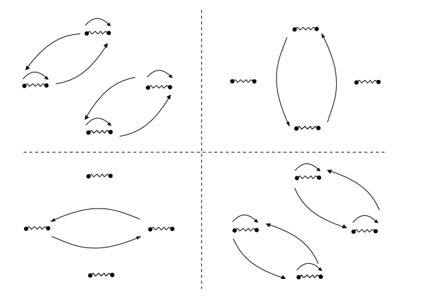
Figure 2: The action of the braidings on the branch-points for SO(5).

Represented on $(a_{D}^{i},a_{i})$, using the reflection symmetry, the monodromy matrices corresponding to the braidings in the figure can be found to be

$$M_{1}=\pmatrix{0&1&-1&1\cr 1&0&1&-1\cr 0&0&0&1\cr 0&0&1&0\cr}, M_{2}=\pmatrix{1&0&0&0\cr 0&-1&0&-1\cr 0&0&1&0\cr 0&0&0&-1\cr},$$

$$M_{1}M_{2}M_{1}^{-1}=\pmatrix{-1&0&-1&-2\cr 0&1&2&0\cr 0&0&-1&0\cr 0&0&0&1\cr}, M_{2}^{-1}M_{1}M_{2}=\pmatrix{0&-1&-1&-2\cr-1&0&0&-1\cr 0&0&0&-1\cr 0&0&-1&0\cr},$$ (30)

respectively. We must now now compare with the result obtained from working with the semi-classical action. It is easy to see that the results agree. $M_{1}$ and $M_{2}$ are simple monodromies of the form (14).

3.4 The special Coxeter monodromies

Argyres and Faraggi [2] used special monodromies to check the semi-classical monodromies of $SU(n)$ curves. To use their arguments in a more general context we rephrase them as follows.

We have noted that all semi-classical monodromies can be generated by composition of $r$ simple monodromies $M_{k}$. Therefore, when all monodromies of the rank $r-1$ sub-groups obtained by removing a vertex from a rank $r$ Dynkin diagram are known, it is enough to check a single new semi-classical monodromy for the rank $r$ group. The simplest monodromies which do not belong to any such sub-groups correspond to braids

$$t_{C}=t_{1}t_{2}\ldots t_{r}.$$ (31)

One can prove that the effect of a permutation of the factors of the product is only to give a braid group element which is conjugate to $t_{C}$. The argument is a copy of a standard argument [8] for the corresponding element in the Weyl group, the Coxeter element. We therefore call $t_{C}$ a Coxeter braid.

We have already checked that the curve (16) gives the correct hierarchy of subgroups, and that it works for low rank groups. We can then prove by induction that composition of semi-classical monodromies works properly, if only the special rank $r$ monodromy corresponding to the Coxeter braid is given correctly by the curve.

A great advantage of using Coxeter braids is that their monodromies are easy to calculate from the curve by perturbation theory in small $\Lambda$. The $SO(2r+1)$ curve (16) has branch points at the roots of the right-hand side polynomial in $x$. For $\Lambda=0$ there are $2r$ double roots at $x=\pm b_{k}$. Let $b_{1}$ be a complex number such that $0<{\rm Arg}b_{1}<\pi/2r$, and set

$$b_{k+1}=b_{k}e^{ik(-1)^{k}\pi/r},k=1,\ldots,r-1.$$ (32)

Then the vector $b$ lies in the fundamental domain, and our previous results can be applied to monodromies with $b$ as a base point. For small non-zero $\Lambda$ the double roots on a circle split into $2r$ pairs of branch points at

$$b^{\pm}_{k}\approx b_{k}(1\pm c({\Lambda\over b_{k}})^{2r-1}),$$ (33)

where $c$ is a real-valued constant. It is convenient to choose a basis of cycles analogous to the $SO(5)$ cycles of figure 1, with cuts between the branch points of a pair, $\gamma$ and $\gamma^{\prime}$ cycles around the branch cuts and $\gamma_{D}$ cycles between opposite branch cuts.

One finds that a Coxeter braid $t_{r}t_{r-2}\ldots t_{r-3}t_{r-1}$ rotates the positions of pairs $b_{k}$ an angle $\pi/r$ while the cuts are rotated an angle $2\pi-2\pi/r$ in the opposite direction. From this we have checked directly the special monodromies of $SO(5)$ and $SO(7)$, but it is much easier to check their $2r$’th power. Then all $b$’s are rotated a full turn and their cuts rotate $2r-2$ times in the opposite direction. This will cause a $2\gamma_{D}^{i}$ cycle to wind $2(2r-2+1)$ times around $\gamma_{i}$ and the same number of times around $\gamma_{i}^{\prime}$. Each sheet is contributing, hence the factor of $2$. From this it follows that this power of the special monodromy is given by

$$\pmatrix{{\mathbbm{1}}&-2C_{2}{\mathbbm{1}}\cr 0&{\mathbbm{1}}\cr}$$ (34)

for any $SO(2r+1)$ group, as is to be expected from (12).

4 Strong coupling monodromies

Let us now consider the singular sub-manifolds of the moduli space where the discriminant vanishes. Parametrized by the symmetric polynomials $u$ and $v$, the $SO(5)$ curve is given by

$$y^{2}=(x^{4}-ux^{2}+v)^{2}-\Lambda^{6}x^{2}.$$ (35)

The discriminant vanishes when $v=0$ or for $u$ and $v$ such that

$$x^{4}-ux^{2}+v = \pm\Lambda^{3}x$$

$$x(4x^{2}-2u) = \pm\Lambda^{3}$$ (36)

has a solution. One may study, for instance, the three dimensional submanifold $Im(v)=0$. All $Re(v)=const.$ planes (if $Re(v)\neq 0$) can be shown to cut through four singular submanifolds. As $Re(v)=0$ is approached, one of these singular submanifolds will drift of towards $|u|=\infty$, and only three will cut the $Re(v)=0$ plane. They will do so in the points

$$u={3\over 4^{1/3}}\Lambda^{2}e^{{2\pi i\over 3}n}$$ (37)

where $n=1,2,3$ respectively. One can check that each intersection-point corresponds to a pair of mutually local dyons becoming massless. The three intersection-points are related by a ${\mathbbm{Z}}_{3}$-symmetry and correspond to the three vacua of a $N=1$ $SO(5)$ theory where we have confinement or oblique confinement. That these vacua are represented in the $N=2$ theory, is an important check of our curve. We might add that there is another triplet of intersections that are not candidates for $N=1$ vacua. These are at

$$u={3\Lambda^{2}\over 2}e^{{2\pi i\over 3}n},\;\;\;v=-{3\Lambda^{4}\over 16}e^{{4\pi i\over 3}n}$$ (38)

for $n=1,2,3$.

A strong coupling monodromy is obtained by encircling some singular sub-manifold. The semi-classical monodromies can often be obtained by taking pairs of such strong coupling monodromies. A strong coupling monodromy typically splits some pair of branch points. The semi-classical monodromies, as we have seen, leave the pairs together. Let us consider an example!

To find the strong coupling monodromies one can use the Picard- Lefshetz theorem. This is based on the vanishing cycles and states that ${\cal M}_{\nu}\gamma=\gamma+\langle\gamma,\nu\rangle\nu$ where $\gamma$ is an arbitrary cycle on which the monodromy ${\cal M}_{\nu}$ is acting and $\nu$ the vanishing cycle. A vanishing cycle is a cycle that encircles a pair of branch points that move together as some singular sub-manifold is approached. A pair of such vanishing cycles are shown in figure 3.

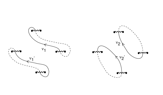
Figure 3: Vanishing cycles for two strong coupling monodromies for SO(5).

Note that due to the reflection symmetry, each vanishing cycle is doubled. We hence have to be careful when we use the Picard-Lefshetz theorem. In fact, we have

$${\cal M}_{\nu}\gamma=\gamma+\langle\gamma,\nu\rangle\nu+\langle\gamma,\nu^{\prime}\rangle\nu^{\prime}.$$ (39)

Alternatively one can trace the cycles as the branch points move as we did for the semi-classical case. The strong coupling monodromies so obtained are

$${\cal M}_{1}=\pmatrix{0&-1&-1&-2\cr-2&-1&-2&-4\cr 1&1&2&2\cr 1&1&1&3\cr}$$ (40)

and

$${\cal M}_{2}=\pmatrix{1&0&0&0\cr-1&0&0&-1\cr 1&1&1&1\cr 1&1&0&2\cr}.$$ (41)

Multiplying them together as ${\cal M}_{2}{\cal M}_{1}$ gives the last of the monodromies in eq. (30) as it should. It is easy to check that ${\cal M}_{1}$ is associated with a dyon with charge vector $(\bar{g}_{1},\bar{q}_{1})=(1,-1,1,-2)$ and ${\cal M}_{2}$ with a dyon with charge vector $(\bar{g}_{2},\bar{q}_{2})=(1,-1,0,-1)$. This can be read off directly from the corresponding vanishing cycle or by noting that these charge-vectors are left eigen-vectors with eigen-value one for the respective monodromy matrice.

Similarly, one can work out the details for the other singular sub-manifolds and dyons.

5 Conclusions

In this paper we have extended the construction for $SU(N_{c})$ treated in [1-4] to the case $SO(2r+1)$. A new and perhaps unexpected feature of the complex curves involved in our solutions is that the genus is larger than the rank of the group. This is possible because of additional symmetries of the curves. Clearly it is important to generalize the solutions to arbitrary groups. We believe that our general description of the semi-classical monodromies can be of help in such constructions.

We wish to thank T. Ekedahl, J. Kalkkinen, U. Lindström, and H. Rubinstein for their comments.

References

- [1] N. Seiberg and E. Witten, Nucl. Phys. B426 (1994) 19, B431 (1994) 484.
- [2] P.C. Argyres and A.E. Faraggi, preprint IASSNS-HEP-94/94, hep-th/9411057.
- [3] A. Klemm, W. Lerche, S. Yankielowicz and S. Theisen, preprint CERN-TH.7495/94, LMU-TPW 94/16, hep-th/9411048; preprint CERN-TH.7538/94, LMU-TPW 94/22, hep-th/9412158.
- [4] M.R. Douglas and S.H. Shenker, preprint RU-95-12, hep-th/9503163.
- [5] K. Intriligator and N. Seiberg, preprint RU-95-3,IASSNS-HEP-95/5, hep-th/9503179.
- [6] D. Amati, K. Konishi, Y. Meurice, G.C. Rossi and G. Veneziano, Phys. Rep. 162, No. 4 (1988) 169.
- [7] V.I. Arnol’d, V.A. Vasil’ev, V.V. Goryunov and O.V. Lyashko, Singularity Theory I, Dynamical Systems VI, Encyclopaedia of Mathematical Sciences Vol. 6. Springer-Verlag 1993.
- [8] J.E. Humphreys, Reflection Groups and Coxeter Groups. Cambridge University Press 1990.