Static skyrmions in (2+1) dimensions

Abstract

In the spirit of previous papers, but using more general field configurations, the non-linear $O(3)$ model in (2+1)-D, modified by the addition of both a potential-like term and a Skyrme-like term, is considered. The instanton solutions are numerically evolved in time and some of their stability properties studied. They are found to be stable, and a repulsive force is seen to exist among them. These results, which are restricted to the case of zero-speed systems, confirm those obtained in previous investigations, in which a similar problem was studied for a different choice of the potential-like term.

1 Introduction

In the past few years, $\sigma$-models in low dimensions have become an increasingly important area of research, often arising as approximate models in the contexts of both particle and solid state physics. They have been used in the construction of high-$T_{c}$ superconductivity and the quantum Hall effect; in two Euclidean dimensions, they appear to be the low-dimensional analogues of four-dimensional Yang-Mills theories. But only very special $\sigma$-models in (2+1)-D are integrable [1], and the physically relevant Lorentz-invariant models are not amongst them; in these cases, recourse to numerical evolution must be made. The simplest Lorentz-invariant model in (2+1)-D is the $O(3)$ model, which involves three real scalar fields, $\phi$($x^{\mu}$)$\equiv${$\phi_{a}$($x^{\mu}$), $a$=1,2,3}, with the constraint that $\phi$ lies on the unit sphere $S^{(\phi)}_{2}$:

$$\mbox{\boldmath$\phi.\phi$}=1.$$ (1)

Subject to this constraint, the Lagrangian density and the corresponding equations of motion are

$${\cal L}_{\sigma}=\frac{1}{4}(\partial_{\mu}\mbox{\boldmath$\phi$}).(\partial^{\mu}\mbox{\boldmath$\phi$}),$$ (2)

$$\partial^{2}_{t}\mbox{\boldmath$\phi$}=[-(\partial_{t}\mbox{\boldmath$\phi$})^{2}+(\partial_{x}\mbox{\boldmath$\phi$})^{2}+(\partial_{y}\mbox{\boldmath$\phi$})^{2}]\mbox{\boldmath$\phi$}+\partial^{2}_{x}\mbox{\boldmath$\phi$}+\partial^{2}_{y}\mbox{\boldmath$\phi$}.$$ (3)

Note that we are concerned with the model in (2+1)-D: $x^{\mu}\equiv(x^{0},x^{1},x^{2})=(t,x,y)$, with the speed of light set equal to unity.

An alternative and convenient formulation of the model is in terms of one independent complex field, $W$, related to the fields $\phi_{a}$ via

$$W=\frac{1-\phi_{3}}{\phi_{1}+i\phi_{2}}.$$ (4)

In this formulation, the Lagrangian density and the corresponding equations of motion read (asterisk denotes complex conjugation)

$${\cal L}_{\sigma}=\frac{\partial_{\mu}W\partial^{\mu}W^{*}}{(1+|W|^{2})^{2}},$$ (5)

and

$$\partial^{2}_{t}W=\partial^{2}_{x}W+\partial^{2}_{y}W+\frac{2W^{*}[(\partial_{t}W)^{2}-(\partial_{x}W)^{2}-(\partial_{y}W)^{2}]}{1+|W|^{2}}.$$ (6)

The problem is completely specified by giving the boundary conditions. As usual we take

$$\lim_{r\rightarrow\infty}\mbox{\boldmath$\phi$}(r,\theta,t)=\mbox{\boldmath$\phi$}_{0}(t),$$ (7)

where $\phi$₀($t$) is independent of the polar angle $\theta$. In (2+1)-D this condition ensures a finite potential energy, whereas in two Euclidean dimensions, i.e., when $\phi$ is independent of time, this leads to the finiteness of the action, which is precisely the requirement for quantization in terms of path integrals. As shown by several people [2, 3], any rational function $W(z)$ or $W(z*)$, where $z=x+iy$, is a static solution of eq. (6). These are the instantons of the model, and can be regarded as static solitons of the same model in (2+1)-D. The simplest one-soliton solution, $W=\lambda z$ ($\lambda$ is a free parameter determining the size of $W$), has been numerically studied by Leese et.al [4]. When viewed as an evolving structure in (2+1)-D, the soliton has been found to be unstable; any small perturbation, either explicit or introduced by the discretization procedure, changes its size. This instability is associated with the conformal invariance of the $O(3)$ Lagrangian in two dimensions.

The $O(3)$ solitons, however, can be stabilized through a judicious introduction of a scale into the model, thereby breaking its conformal invariance. As explained below, in the present article we study this problem following the methods of a previous investigation [5], but considering a different potential-like term and restricting ourselves to the systems initially at rest.

2 Skyrme model in (2+1) dimensions

Using the $W$-formulation, our Skyrme model is defined by the Lorentz-invariant Lagragian density

$${\cal L} = {\cal L}_{\sigma}$$ (8)

$$- 2\theta_{1}[\frac{(\partial_{t}W^{*}\partial_{y}W-\partial_{t}W\partial_{y}W^{*})^{2}+(\partial_{t}W^{*}\partial_{x}W-\partial_{t}W\partial_{x}W^{*})^{2}}{(1+|W|^{2})^{4}}$$

$$- \frac{(\partial_{x}W^{*}\partial_{y}W-\partial_{x}W\partial_{y}W^{*})^{2}}{(1+|W|^{2})^{4}}]$$

$$- 4\theta_{2}\frac{|W-\lambda|^{8}}{(1+|W|^{2})^{4}},$$

where ${\cal L}_{\sigma}$ is given by eq. (5) and $\theta_{1}$,$\theta_{2}$ are real parameters with dimensions of length squared and inverse length squared, respectively; they introduce a scale into the model, which is no longer conformal invariant. If the size of the solitons is appropriately chosen, it is energetically unfavourable for the solitons to change it. The $\theta_{1}$-term is the (2+1)-D analogue of the Skyrme term, whereas the $\theta_{2}$-term is a potential-like one. Unlike the former, the latter term is highly nonunique [6].

The field equation corresponding to the above Lagrangian can be cast into the form

$$W_{tt} = W_{xx}+W_{yy}+\frac{2W^{*}[(W_{t})^{2}-(W_{x})^{2}-(W_{y})^{2}]}{1+|W|^{2}}$$ (9)

$$- \frac{4\theta_{1}}{(1+|W|^{2})^{2}}[2W^{*}_{tx}W_{t}W_{x}+2W^{*}_{ty}W_{t}W_{y}-2W^{*}_{xy}W_{x}W_{y}$$

$$+ W^{*}_{xx}(W_{y}^{2}-W_{t}^{2})+W^{*}_{yy}(W_{x}^{2}-W_{t}^{2})-W^{*}_{tt}(W_{x}^{2}+W_{y}^{2})$$

$$+ W_{xx}(|W_{t}|^{2}-|W_{y}|^{2})+W_{yy}(|W_{t}|^{2}-|W_{x}|^{2})+W_{tt}(|W_{x}|^{2}+|W_{y}|^{2})$$

$$+ W_{xy}(W_{x}^{*}W_{y}+W_{y}^{*}W_{x})-W_{tx}(W_{t}^{*}W_{x}+W_{x}^{*}W_{t})-W_{ty}(W_{t}^{*}W_{y}+W_{y}^{*}W_{t})$$

$$+ \frac{2W}{1+|W|^{2}}((W^{*}_{t}W_{y}-W^{*}_{y}W_{t})^{2}+(W^{*}_{x}W_{t}-W^{*}_{t}W_{x})^{2}-(W^{*}_{x}W_{y}-W^{*}_{y}W_{x})^{2})]$$

$$+ \frac{16\theta_{2}|W-\lambda|^{2}}{(1+|W|^{2})^{3}},$$

where the notation $W_{x}\equiv\partial_{x}W$, $W_{xx}\equiv\partial_{x}^{2}W$, etc., has been used.

It is straightforward to check that

$$W=\lambda\frac{z-a}{z-b}$$ (10)

is a static solution of eq. (9), provided the following relation holds:

$$\lambda=\frac{\sqrt[4]{2\theta_{1}/\theta_{2}}}{a-b}.$$ (11)

Now $\lambda$, which characterizes the size of the instanton $W$, is no longer a free parameter. It is fixed by eq. (11). The instanton, with its size thus fixed, is usually referred to as a ‘skyrmion’. Unlike the ordinary $O(3)$ case [4], where the instanton changes its size as time elapses, we expect our skyrmion to be stable. In reference 5, a similar question was studied using $-4\theta_{2}/(1+|W|^{2})^{4}$ for the potential-like term, with the Skyrme field given by $\lambda z$, where $\lambda=\sqrt[4]{2\theta_{1}/\theta_{2}}$.

3 Numerical setup and results

To perform our numerical simulations we employ the fouth-order Runge-Kuttamethod, and approximate the spatial derivatives by finite differences; the Laplacian is evaluated using the nine-point formula. All computations were performed on the workstations at Durham, on a fixed 201$\times$201 lattice with spatial and time steps $\delta x$=$\delta y$=0.02 and $\delta t$=0.005. Every few iterations we rescaled the fields $\mbox{\boldmath$\phi$}\rightarrow\mbox{\boldmath$\phi$}/\sqrt{\mbox{\boldmath$\phi.\phi$\,}\,}\,$. We also included along the boundary a narrow strip to absorb the various radiation waves, thus reducing their effects on the skyrmions via the reflections from the boundary. As time elapses, this absorption of radiation manifests itself through a small decrease of the total energy, which gradually stabilizes as the radiation waves are gradually absorbed.

We choose the parameters to have the values: $\theta_{1}$=0.015006250, $\theta_{2}$=0.1250, $a$=0.75 and $b$=0.05 which, according to eq. (11), set $\lambda$=1.

3.1 Results for one skyrmion

The numerical evolution shows that the skyrmion’s shape, of which a representative picture is given in the upper half of figure 1, practically does not change as a function of time. The maximum of the total energy density, which is related to the soliton size, starts off at the value 128.5 and, after some radiation waves are emitted, stabilizes at $\approx$ 129.5 (see lower half of figure 1). This is in agreement with the analytical result, as the expression for the maximum of the total energy density, namely, $E_{max}=\varepsilon(1+\theta_{1}\varepsilon)$, $\varepsilon=8(|\lambda|^{2}+1)^{2}/|\lambda(a-b)|^{2}$, yields 129.3, the ‘canonical size’.

In figure 2 are exhibited some kinetic energy density waves. They propagate out to the boundary at the speed of light, leaving the region where the skyrmion is located essentially free of kinetic energy. The smallness of the kinetic energy indicates that the field given by eq. (10) remains almost perfectly static. For example, the amplitude of the total energy density, at $t$=0, is positioned at $z_{max}$=(0, 0.4000) and, for $t$=10, it has been slowly shifted to (0, 0.4013).

So, as expected, our skyrmion appears to be stable under perturbations brought about by the discretization procedure. These results agree with those of reference [5], where the skyrmion was positioned at the centre of the grid, i.e., $z_{max}$=0, which, as one can easily check, corresponds to a skyrmion given by $W=\lambda z$ or $W=1/\lambda z$.

In order to study the stability problem further, we are currently performing simulations with the same $\theta_{i}$-values but setting $\lambda\neq 1$. This corresponds to initial conditions that are no longer those of the static solution. We hope some concrete results will be available in the future.

3.2 Results for two skyrmions

Let us now consider the case where two instantons are put on a lattice. We consider the field

$$W=\lambda\frac{z-a}{z-b}\frac{z+c}{z+d},$$ (12)

with $\lambda$=1, $a=c=0.75$, $b=d=0.05$ and let it evolve. One can readily verify that the above field configuration is not a solution of the equations of motion, and hence it evolves when started off at rest.

Our simulations have shown that, at the initial time, $E_{max}$ is well above the canonical size as determined in the last sub-section. As soon as the evolution in time begins the solitons shake off some kinetic energy and alter their size by getting broader; $E_{max}$ decreases and then undergoes damped-oscillations around a value very close to the canonical one. As this happens, the solitons slowly move away from each other, exhibiting the presence of a repulsive force between them. By $t\approx 8$, the amplitude of the above-mentioned oscillations is quite small, and $E_{max}$ eventually stabilizes near the expected canonical value. Typical pictures for this case are displayed in figures 3 and 4.

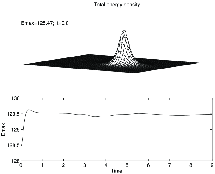
Figure 1: Total energy density for one skyrmion at the initial time and the evolution of its peak.

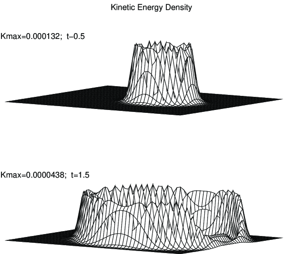
Figure 2: Kinetic waves travelling towards the boundary.

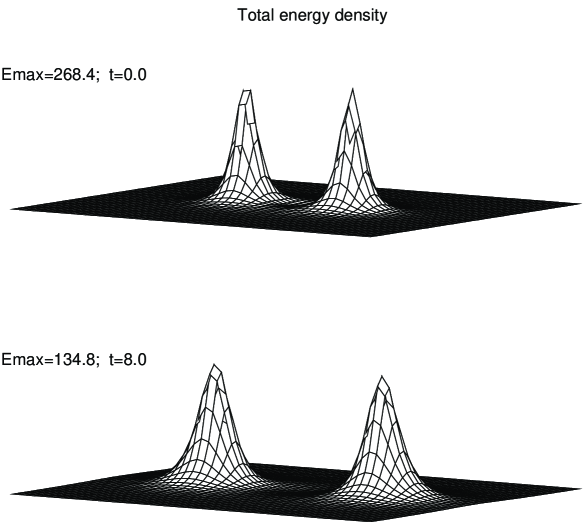
Figure 3: Two skyrmions. A repulsive force exists between them.

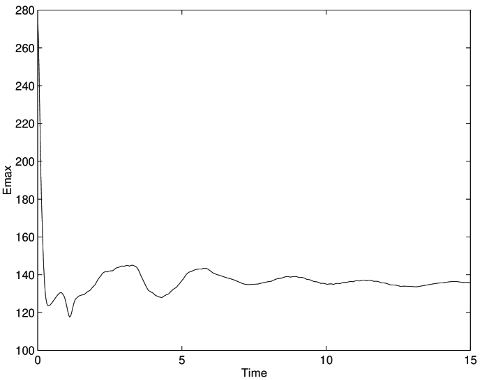
Figure 4: Evolution of the maximum of the total energy density for the two-skyrmions case.

4 Conclusions

We have performed a numerical study of the time evolution of the general one-instanton solutions of our version of the Skyrme model in (2+1)-D, confirming some of the properties previously seen in other versions of the model. The extra terms added to the ordinary non-linear $O(3)$ model break its conformal invariance and stabilize the solitons. The changes of soliton size and position are negligible as time progresses. Also, the time evolution of the two-skyrmion configuration has showed us that, like in the previously studied model, the forces between the skyrmions are repulsive.

A paper on the scattering properties of our skyrmions will be available in not too distant a future.

Acknowledgements

R. J. Cova is deeply indebted to Universidad del Zulia and Fundación Gran Mariscal de Ayacucho for their joint grant supporting his Ph.D. studies in Durham. He also wishes to thank David Bull for helpful discussions.

References

- [1] Ward R. S. 1988 Nonlinearity 1 671.
- [2] Belavin A. A. and Poliakov A. M. 1975 JETP letters 22 245.
- [3] Woo G. 1977 J. Math. Phys. 18 1264.
- [4] Leese R. A., Peyrard M. and Zakrzewski W. J. 1990 Nonlinearity 3 387.
- [5] Leese R. A., Peyrard M. and Zakrzewski W. J. 1990 Nonlinearity 3 773.
- [6] Azcárraga J. A. de, Rashid N. S. and Zakrzewski W. J. 1991 J.Math.Phys. 32 1921.