ON SOME NEW BLACK STRING SOLUTIONS IN THREE DIMENSIONS

Abstract

We derive several new solutions in three-dimensional stringy gravity. The solutions are obtained with the help of string duality transformations. They represent stationary configurations with horizons, and are surrounded by (quasi) topologically massive Abelian gauge hair, in addition to the dilaton and the Kalb-Ramond axion. Our analysis suggests that there exists a more general family, where our solutions are special limits. Finally, we use the generating technique recently proposed by Garfinkle to construct a traveling wave on the extremal variant of one of our solutions.

I Introduction

Recently we have witnessed a surge of interest in lower-dimensional theories of gravity, after the realization that many of them contain structures with horizons [1]-[7]. Investigation of these models is motivated by the hope that we may be able to gain more information about the physics of realistic four-dimensional black holes, since mathematical difficulties subside dramatically in fewer dimensions. This approach appears to be particularly fruitful in lower-dimensional stringy gravity, where the facilities of string theory provide us with very powerful tools to study black holes in the classical limit and beyond [8]-[20]. Resorting to these techniques, we may be able to tackle in a systematic way some of the long-standing conundrums of black hole physics. For example, it has been demonstrated that string theory may have the potential to cure some of the singularity problems which plague the classical theory[21].

In this paper we shall contribute several new black hole-like solutions to the existing bestiary. We shall employ the Abelian duality symmetry as our main tool to obtain them [8]-[15]. Such symmetries represent a stringy generalization of standard toroidal symmetries, stemming from the presence of commuting translational Killing vectors in a gravitational background. They can be combined and employed to derive new background solutions. The general procedure is dubbed twisting, or $O(d,d)$ boosting, after the complete group of twisting transformations [10, 11, 12]. At the level of the background field theory on target space, after integrating out Killing coordinates à la Kaluza-Klein, this is realized as a symmetry of the action under mixing of the Kaluza-Klein matter fields with the metric. Although the action is invariant under this group, solutions are not, because they employ specific initial conditions. Therefore, the twisting transformations can generate new classical solutions. It must be kept in mind, however, that dual solutions may not represent different string physics, but merely be different pictures of the same string theory, which for example occurs when one dualizes with respect to the translation of a compact coordinate [14]. Moreover, the full $O(d,d)$ group also contains diffeomorphisms and Kalb-Ramond field gauge transformations, which must be modded out [11]. Thus, the space of classical solutions is spanned by the orbits of the $O(d,d)$ group, modulo diffeomorphisms and Kalb-Ramond gauge transformations.

This symmetry is further extended to $O(d,d+n)$ in the presence of $n$ Abelian gauge fields [9]. We will use this extended boost symmetry to obtain two new three-dimensional (3D) families of asymptotically flat solutions. Our families are obtained by, respectively, “twisting in” the gauge field on the black string of Horne and Horowitz [3], and the axion on the 2D electrically charged black hole crossed with a flat line [4]. They are characterized by three parameters, and for certain ranges of the parameters they represent different stationary, gauge charged configurations with regular horizons. Some of their properties are quite remarkable. Namely, although all our non-extremal black strings possess a scalar curvature singularity, which must be included in the manifold because it is spacelike geodesically incomplete, this singularity is quite harmless for pointlike observers. The manifold is null and timelike geodesically complete, since for arbitrary initial conditions at infinity all causal geodesics have a turning point before reaching the singularity except for one null geodesic, which comes arbitrarily close to the singularity but never reaches it for a finite value of the affine parameter. The first family possesses an interesting non-singular extremal limit, different from the extremal limits of previously known solutions in that it has one hypersurface orthogonal null Killing vector, and nonvanishing gauge hair. Therefore, we can further extend this solution to include a traveling wave, using the generating technique proposed recently by D. Garfinkle in the context of string gravity [29]. Our first family also contains a subclass of solutions with interesting global properties. These solutions are without curvature singularities, with spatial hypersurfaces looking like a “cigar”, approaching asymptotically ${\bf R}\times{\bf S}^{1}$. However, the angular variable is “bolted” to time, and hence near the origin there appear closed timelike curves.

The second family has, curiously, a critical value of the boost parameter and a black string with two different extremal limits. The critical boost gives the stringy version of the 3D black hole [5, 6]. Away from this critical boost we find another family of black strings, which displays a peculiar combination of properties of both black strings and four dimensional black holes. Particularly interesting is the presence of the ergosphere, which arises entirely due to the axion and electric charges. Furthermore, this black string has two extremal limits. One of them corresponds to taking the critical value of the boost, but after a coordinate transformation, in a fashion familiar from the static black string case. The other extremal limit is reminiscent of the extremal Kerr-Newman case, and represents a gauge charged black string, with ergosphere but without null Killing vectors.

The paper is organized as follows. In the next section, we will lay out mathematical background for the subsequent study, explaining our approach and deriving various forms of the solutions. Detailed investigation of the solutions will be presented in section III. Section IV contains the derivation of the traveling wave solution, using Garfinkle’s techniques. The final section offers our conclusions and presents arguments that suggest the existence of a larger family of 3D black objects which continually interpolate between our two solutions, as well as the Horne-Horowitz and the stringy BTZ solutions.

II Generating Solutions

The effective action of string theory describing dynamics of massless bosonic background fields to the lowest order in the inverse string tension $\alpha^{\prime}$ is, in the world-sheet frame [10]-[12],[23],

$$S~{}=~{}\int d^{d+1}x\sqrt{g}e^{-\Phi}\big{(}R+\partial_{\mu}\Phi\partial^{\mu}\Phi-{1\over 12}H_{\mu\nu\lambda}H^{\mu\nu\lambda}-{\alpha^{\prime}\over 4}F^{N}{}_{\mu\nu}F^{N}{}^{\mu\nu}+2\Lambda\big{)}.$$ (1)

The action above is written in Planck units $\kappa^{2}=1$. Here $~{}F^{N}{}_{\mu\nu}=\partial_{\mu}A^{N}{}_{\nu}-\partial_{\nu}A^{N}{}_{\mu}~{}$ are field strengths of $n$ Abelian gauge fields $A^{j}{}_{\mu}$, $~{}H_{\mu\nu\lambda}=\partial_{\lambda}B_{\mu\nu}+{}~{}cyclic~{}permutations~{}-({\alpha^{\prime}/2})\Omega_{M}{}_{\mu\nu\lambda}~{}$ is the field strength associated with the Kalb-Ramond field $~{}B_{\mu\nu}~{}$ and $~{}\Phi~{}$ is the dilaton field. The Maxwell Chern-Simons form $\Omega_{M}{}_{\mu\nu\lambda}=\sum_{N}A^{N}{}_{\mu}F^{N}{}_{\nu\lambda}+~{}cyclic~{}permutations~{}$ appears in the definition of the axion field strength due to the Green-Schwarz anomaly cancellation mechanism, and can be understood as a model-independent residue after dimensional reduction from ten-dimensional superstring theory [24]. In fact, this term is a necessary ingredient of the theory if one wants to ensure the $O(d,d+n)$ invariance, as shown by Maharana and Schwarz [12]. The $n$ Abelian gauge fields should be thought of as the components of a non-Abelian gauge field ${\bf A}$ residing in the Cartan subalgebra of the gauge group, while the rest have been set equal to zero. For convenience we will set $\alpha^{\prime}=1$.

In what follows we will be considering only those extrema of (1) that possess $d$ commuting isometries, that is, we will be considering field configurations of the form

$$ds^{2} = \Gamma(r)~{}dr^{2}+G_{jk}(r)~{}dx^{j}dx^{k},$$ (2)

$$B = \frac{1}{2}~{}B_{jk}(r)dx^{j}\wedge dx^{k},$$ (3)

$$A^{N} = A^{N}{}_{j}(r)dx^{j},$$ (4)

$$\Phi = F(r),$$ (5)

where $G_{jk}(r)$ is the metric of a $d$ dimensional submanifold of signature $d-2$. In this case the action (1) can be rewritten in the manifestly $O(d,d+n)$ invariant form [10, 11, 12]

$$S_{eff}~{}=~{}\int dr\sqrt{\Gamma}e^{-\phi}\Big{(}{1\over\Gamma}\phi^{\prime 2}+{1\over 8\Gamma}\mbox{Tr}\bigl{(}{\cal M}^{\prime}{\cal L}\bigr{)}^{2}+2\Lambda\Big{)},$$ (6)

where the prime denotes the derivative with respect to $r$. Note that the physical dilaton $\Phi$ has been replaced by the effective dilaton $\phi=\Phi-(1/2)\ln|\det G|$ after dimensional reduction. Matrices $~{}{\cal M}~{}$ and $~{}{\cal L}~{}$ which appear in the action (6) are defined by

$${\cal M}~{}=~{}\pmatrix{g^{-1}&-g^{-1}C&-g^{-1}A\cr-C^{T}g^{-1}&g+a+C^{T}g^{-1}C&A+C^{T}g^{-1}A\cr-g^{-1}A&A+C^{T}g^{-1}A&{\bf 1}_{n}+A^{T}g^{-1}A\cr},$$ (7)

(8)

$$~{}~{}~{}~{}~{}~{}~{}~{}~{}~{}~{}~{}~{}~{}~{}~{}~{}~{}~{}{\cal L}~{}=~{}\pmatrix{~{}0~{}&{\bf 1}_{d}&~{}0~{}\cr{\bf 1}_{d}&~{}0~{}&~{}0~{}\cr{}~{}0~{}&~{}0~{}&{\bf 1}_{n}\cr}.$$ (9)

Here $~{}g~{}$ and $~{}b~{}$ are $~{}d\times d~{}$ matrices defined by the dynamical degrees of freedom of the metric and the axion:$~{}g~{}=~{}\bigl{(}G_{jk}\bigr{)}$ and $b~{}=~{}\bigl{(}B_{jk}\bigr{)}$. The matrix $A$ is a $~{}d\times n~{}$ matrix built out of the gauge fields: $A_{kN}~{}=~{}A^{N}{}_{k}$. The matrices $a$ and $C$ are defined by $a=AA^{T}$ and $C=(1/2)a+b$ respectively, and $~{}{\bf 1}_{d}~{}$ and $~{}{\bf 1}_{n}~{}$ are the $d$ and $n$ dimensional unit matrices. Note that ${\cal M}^{T}={\cal M}$ and ${\cal M}^{-1}={\cal L}{\cal M}{\cal L}$. Thus we see that ${\cal M}$ is a symmetric element of $O(d,d+n)$. Therefore a cogradient $O(d,d+n)$ rotation ${\cal M}\rightarrow\Omega{\cal M}\Omega^{T}$ is a symmetry of the action, and the equations of motion, because it represents a group motion which changes $\cal M$ while maintaining its symmetry property.

In this paper we will apply this technique to several well-known solutions of stringy gravity to the lowest order in the inverse string tension expansion, describing black strings. Specifically, we will use the black string family discovered by Horne and Horowitz [3], as well as the 2D electrically charged black hole crossed with a flat line, discussed by McGuigan et al. [4]. We start with the black string solution, given by [3]:

$$ds^{2}=\frac{dr^{2}}{2\Lambda(r-m)(r-\frac{Q^{2}}{m})} + (1-\frac{Q^{2}}{mr})dx^{2}-(1-\frac{m}{r})dt^{2},$$ (10)

$$B=\frac{Q}{r}dx\wedge dt, ~{}~{}~{}~{}~{}~{}~{}~{}A=0,$$ (11)

$$e^{-\Phi} = \sqrt{2\Lambda}r.$$ (12)

Following the prescription outlined above, and using

$$\Omega=\left(\matrix{1&0&0&0&0\cr 0&(1+c)/2&0&(1-c)/2&-s/\sqrt{2}\cr 0&0&1&0&0\cr 0&(1-c)/2&0&(1+c)/2&s/\sqrt{2}\cr 0&-s/\sqrt{2}&0&s/\sqrt{2}&c\cr}\right),$$ (13)

where $c=\cosh(2\alpha)$ and $s=-\sinh(2\alpha)$, we obtain the new solution

$$ds^{2} = \frac{d\hat{r}^{2}}{2\Lambda(\hat{r}-m\hat{c}^{2})(\hat{r}-m\hat{s}^{2}-Q^{2}/m)}+\frac{\hat{r}-m\hat{s}^{2}-Q^{2}/m}{\hat{r}-m\hat{s}^{2}}dx^{2}~{}~{}~{}~{}~{}~{}$$ (17)

$$~{}~{}~{}~{}~{}~{}~{}~{}~{}~{}~{}~{}~{}~{}~{}~{}~{}~{}~{}~{}~{}~{}~{}~{}~{}~{}~{}~{}~{}~{}~{}-\frac{\hat{r}-m\hat{c}^{2}}{\hat{r}^{2}(\hat{r}-m\hat{s}^{2})}((\hat{r}-m\hat{s}^{2})dt-\hat{s}^{2}Qdx)^{2},$$

$$~{}~{}~{}B=\frac{Q\hat{c}^{2}}{\hat{r}}dx\wedge dt,~{}~{}~{}~{}~{}~{}~{}~{}~{}~{}~{}~{}~{}A=-\sqrt{2}\frac{\hat{s}\hat{c}}{\hat{r}}(Qdx+mdt),$$

$$~{}~{}~{}~{}~{}~{}~{}~{}~{}~{}~{}~{}~{}~{}~{}~{}~{}~{}~{}~{}~{}~{}e^{-\Phi}=\sqrt{2\Lambda}\hat{r},$$

where $\hat{c}=\cosh\alpha$, $\hat{s}=-\sinh\alpha$, and $\hat{r}=r+m\hat{s}^{2}$. Clearly, (17) generalizes (10), reducing to it when $\alpha=0$. It is obvious that this solution, like (10), is asymptotically flat in the limit $\hat{r}\rightarrow\infty$. We also find it useful to represent our new solution in terms of the shifted time coordinate $\tau=t+(Q/m)x$ instead of $t$. In this gauge, the axion and the dilaton are the same as above. The gauge field is oriented completely along $d\tau$, and the expressions for it and the metric are given as follows:

$$ds^{2} = \frac{d\hat{r}^{2}}{2\Lambda(\hat{r}-m\hat{c}^{2})(\hat{r}-m\hat{s}^{2}-Q^{2}/m)}+\bigl{(}1-\frac{Q^{2}}{m^{2}}\bigr{)}dx^{2}~{}~{}~{}~{}~{}~{}~{}~{}~{}$$ (20)

$$~{}~{}~{}~{}~{}~{}~{}~{}~{}~{}~{}~{}~{}~{}~{}~{}~{}~{}-2\frac{Q}{m}\bigl{(}1-\frac{m\hat{c}^{2}}{\hat{r}}\bigr{)}dxd\tau-\bigl{(}1-\frac{m\hat{c}^{2}}{\hat{r}}\bigr{)}\bigl{(}1-\frac{m\hat{s}^{2}}{\hat{r}}\bigr{)}d\tau^{2},$$

$$~{}~{}~{}~{}~{}~{}~{}~{}~{}~{}~{}~{}~{}~{}~{}~{}~{}~{}~{}~{}~{}~{}~{}A=-\sqrt{2}\frac{m\hat{s}\hat{c}}{\hat{r}}d\tau.$$

This form is suitable for comparison with our second solution, to be presented shortly, but not useful for the analysis of the causal structure, as can be immediately seen from the fact that $\tau$ is not the asymptotic time coordinate.

We now consider the electrically charged stringy 2D black hole crossed with a flat line ${\bf R}$ [4]:

$$ds^{2}=\frac{d{\rho}^{2}}{2\Lambda({\rho}-\frac{q^{2}}{\mu})({\rho}-\mu)}+ d\xi^{2} -(1-\frac{q^{2}}{\mu\rho})(1-\frac{\mu}{\rho})d\hat{\tau}^{2},$$ (21)

$$B=0,~{}~{}~{}~{}~{}~{}~{}~{}~{}~{}~{} A=-\frac{\sqrt{2}q}{\rho}d\hat{\tau},$$ (22)

$$e^{-\Phi}= \sqrt{2\Lambda} {\rho},$$ (23)

To obtain our other solution we apply another $O(2,3)$ twist to it, with $b$ a real number:

$$\Omega=\left(\matrix{0&1&b&0&0\cr 1&0&0&-b&0\cr 0&0&0&1&0\cr 0&0&1&0&0\cr 0&0&0&0&1\cr}\right).$$ (24)

This yields the following expression:

$$ds^{2} = \frac{d{\rho}^{2}}{2\Lambda({\rho}-\frac{q^{2}}{\mu})({\rho}-\mu)}+\frac{b^{2}({\rho}-M)^{2}-f}{((1-b^{2}){\rho}+Mb^{2})^{2}}d\xi^{2}$$ (26)

$$~{}~{}~{}~{}~{}~{}~{}~{}~{}~{}~{}~{}~{}~{}~{}+\frac{{\rho}^{2}-b^{2}f}{((1-b^{2}){\rho}+Mb^{2})^{2}}d\hat{\tau}^{2}-\frac{2bq^{2}}{((1-b^{2}){\rho}+Mb^{2})^{2}}d\xi d\hat{\tau},$$

$$B = \frac{b({\rho}-M)}{(1-b^{2}){\rho}+Mb^{2}}d\xi\wedge d\hat{\tau},~{}~{}~{}~{}~{}A=-\frac{\sqrt{2}q}{(1-b^{2}){\rho}+Mb^{2}}(d\xi+bd\hat{\tau}),$$ (28)

$$~{}~{}~{}~{}~{}~{}~{}~{}~{}~{}~{}~{}~{}e^{-\Phi}=\sqrt{2\Lambda}((1-b^{2}){\rho}+Mb^{2}),$$

where $f=(\rho-\mu)(\rho-q^{2}/\mu)$ and $M=\mu+\frac{q^{2}}{\mu}$. Note that $b^{2}=1$ represents a special point in the moduli space of this family, as the dilaton field decouples there. Indeed, after a closer look (and some coordinate transformations) we recognize this case as precisely the stringy version of the Banados-Teitelboim-Zanelli (BTZ) [5, 6] black hole. In what follows, for computational purposes we will assume $b>1$ (the sign of $b$ only determines the sign of the axion charge), without any loss of generality, as we will now demonstrate. To start with, the solution (26) can be simplified considerably with some judicious gauge choices. We begin with the coordinate transformation $\hat{r}=(1-b^{2}){\rho}+Mb^{2}$, $x=\xi/\sqrt{b^{2}-1}$, and $t=\hat{\tau}/\sqrt{b^{2}-1}$. We can also apply the axion gauge transformation which shifts the asymptotic value of the axion to zero. In this gauge, the solution takes the form

$$ds^{2} = \frac{d\hat{r}^{2}}{2\Lambda(\hat{r}-\mu b^{2}-\frac{q^{2}}{\mu})(\hat{r}-\mu-\frac{q^{2}b^{2}}{\mu})}+(1-\frac{M}{\hat{r}}-\frac{q^{2}(b^{2}-1)}{\hat{r}^{2}})dx^{2}~{}~{}~{}~{}~{}~{}~{}$$ (32)

$$~{}~{}~{}~{}~{}~{}~{}~{}~{}~{}~{}~{}~{}~{}~{}~{}~{}~{}-(1-\frac{Mb^{2}}{\hat{r}}+\frac{q^{2}(b^{2}-1)b^{2}}{\hat{r}^{2}})dt^{2}-2\frac{bq^{2}(b^{2}-1)}{\hat{r}^{2}}dxdt$$

$$~{}B=\frac{bM}{\hat{r}}dx\wedge dt,~{}~{}~{}~{}~{}~{}~{}~{}~{}~{}~{}~{}~{}A=-\sqrt{2}\frac{q\sqrt{b^{2}-1}}{\hat{r}}(dx+bdt),$$

$$~{}~{}~{}~{}~{}~{}~{}~{}~{}~{}~{}~{}~{}~{}~{}~{}~{}~{}~{}~{}~{}~{}~{}e^{-\Phi}=\sqrt{2\Lambda}\hat{r}.$$

It is straightforward to verify that if $|b|<1$, the same coordinate transformation, followed by Wick rotation $t,x\rightarrow it,ix$, rescaling $\hat{r}\rightarrow\hat{r}/b^{2}$, a constant dilaton shift and the replacement of the parameter $b\rightarrow b^{\prime}=1/b>1$ reduces the form of (26) again to (32). We will defer further discussion of the interpretation of the $|b|<1$ solutions until later.

The solution (32) is also an asymptotically flat configuration with both axion and gauge fields. It is again useful, for easier comparison, to perform another coordinate change, to put this solution in a form similar to (20). The dilaton and axion remain the same as above, while the metric and the gauge field are given as follows:

$$ds^{2} = \frac{d{\hat{r}}^{2}}{2\Lambda({\hat{r}}-\mu b^{2}-\frac{q^{2}}{\mu})({\hat{r}}-\mu-\frac{q^{2}b^{2}}{\mu})}+\bigl{(}1-\frac{1}{b^{2}}\bigr{)}dx^{2}{}~{}~{}~{}~{}~{}~{}$$ (35)

$$~{}~{}~{}~{}~{}~{}~{}~{}~{}~{}~{}~{}~{}~{}-2\frac{1}{b}\bigl{(}1-\frac{Mb^{2}}{\hat{r}}\bigr{)}dxd\tau-(1-\frac{Mb^{2}}{\hat{r}}+\frac{q^{2}(b^{2}-1)b^{2}}{\hat{r}^{2}})d\tau^{2},$$

$$~{}~{}~{}~{}~{}~{}~{}~{}~{}~{}~{}~{}~{}~{}~{}~{}~{}~{}~{}~{}A=-\sqrt{2}\frac{qb\sqrt{b^{2}-1}}{\hat{r}}d\tau.$$

Despite the conspicuous similarity between (20) and (35), we will demonstrate later in our analysis that they are indeed different. This can already be glimpsed, however, by realizing that the matter content of the two configurations is exactly the same once the proper coordinate rescalings are performed, and that since they are stationary and contain a scalar, a vector and the volume form in the $(x,\tau)$ subspace, we are left without any freedom to perform further coordinate transformations which do not alter the form of the matter. Specifically, the fact that the dilaton of both configurations is essentially the radial coordinate, and that $x$ and $\tau$ are Killing coordinates restricts the available coordinate transformations to only linear transformations in the $(x,\tau)$ plane. These in general induce the changes of the two gauge fields $A$ and $B$ which are proportional to the field components themselves. Since the fields are nontrivial, i.e. have non-vanishing field strengths, the changes induced by diffeomorphisms are not pure gauges and hence cannot be removed by gauge transformations. The last step in the argument is the comparison of the two metrics, which shows that they do not match; indeed, if we denote the $(x,\tau)$ parts of the two metrics as $g_{1}$ and $g_{2}$, respectively, we can see that $g_{1}=g_{2}+Cdx^{2}$, for some given constant $C$. Since the horizons are determined by the determinant of these matrices, the above shift induces the corresponding shift in the locations of these surfaces.

In the next section we will investigate causal properties of these solutions. Our analysis will confirm and elaborate upon the argument presented above, that they represent different black strings. Before we close this section, however, we should explain an apparent peculiarity which appears in the gauge sector of the two solutions. Namely, we see that in both (20) and (35) the gauge field looks precisely like the field of a point charge in three spatial dimensions, despite the fact that it lives in two dimensions, where one would expect it to be proportional to the logarithm of the distance from the source. Indeed, such behavior has been noted in Ref. [5], where charged black holes in 3D Einstein-Maxwell theory were studied. The resolution to this lies in the fact that in our background the gauge field acquires the (quasi)topological mass term due to its coupling to the Kalb-Ramond field via the Chern-Simons form [25, 26]. The Kalb-Ramond field is trivially integrable in three dimensions [26], and if non-zero, yields the gauge field mass term. The standard Maxwell equation for the gauge field should be replaced in this case by, in form notation, $d\exp(-\Phi){{}^{*}{\bf F}}=2Q_{A}{\bf F}$, where $Q_{A}$ is the axion charge, defined by $Q_{A}=-\exp(-\Phi){{}^{*}{\bf H}}$; it is straightforward to verify that our backgrounds solve it. It is furthermore interesting to note, that whereas in this case the gauge field is (quasi)topologically massive, the gauge sector of either solution does not represent a gauge anyon, as the Chern-Simons form itself vanishes in both cases.

III Causal Structure

Here we will investigate the structure of the two new solutions presented above. Whereas some aspects of the geometry of these two solutions are remarkably similar, there are interesting differences.

As a warm-up, let us review the static black string (10) of Horne and Horowitz, which will be the basis for comparison. This solution has three metric singularities at $r=m$, $r=Q^{2}/m$ and $r=0$, and obviously there are three different cases, $0<|Q|<m$, $|Q|=m$, and $|Q|>m$. When $0<|Q|<m$, $r=0$ is a scalar curvature singularity and $r=m$ and $r=Q^{2}/m$ are the event and Cauchy horizons respectively. The singularity is “real” in the sense that the manifold is null geodesically incomplete. The causal structure of the solution is qualitatively similar to that of the Reissner-Nordstr$\o$m solution, with the exception that the time-like coordinate inside the Cauchy horizon is $x$ rather than $t$. Thus the 2D Penrose diagrams aren’t completely adequate for the description of the geometry, but they can be used with the proviso that one remembers that the time-like coordinate makes a “right angle” turn on the inner horizon. As a consequence, in this solution there are no static observers inside the Cauchy horizon. This case is summarized in Fig.1.

When $|Q|=m$, the form of the solution (10) breaks down at the (degenerate) horizon $r=m$. It turns out that the coordinate $r$ is not suitable for the extension beyond the event horizon, which appears to be a turning point for all geodesics. To see that the manifold does not end there, the authors use the modified radial coordinate ${r^{\prime}}^{2}=r-m$, and show that the geometry contains an event horizon at $r^{\prime}=0$ but has no singularity (Fig. 2). It is interesting to note that this is identical to the causal structure seen in the extremal Kerr solution along the axis of symmetry [27].

Finally, for the case $|Q|>m$ the authors find that the manifold is completely regular, when using the appropriate radial coordinate ${\tilde{r}}^{2}=r-Q^{2}/m$. It terminates at $\tilde{r}=0$, and the potential conical singularity there is removed by a periodic identification of the spacelike coordinate $x$. Therefore, the spacelike sections have the structure of a “cigar”, looking flat near the origin but asymptotically approaching ${\bf R}\times{\bf S}^{1}$.

Let us now turn our attention to our new solutions. Both (17) and (32) share some of the features of the static black string (10). They are both asymptotically flat configurations with two Killing fields, $\partial_{x}$ and $\partial_{t}$, with infinity described by the limit $\tilde{r}=\ln\hat{r}\rightarrow\infty$, where they approach exponentially fast the linear dilaton vacuum, with flat Minkowski metric and vanishing gauge fields. They also have three metric singularities each, $\hat{r}=m\hat{c}^{2}$, $m\hat{s}^{2}+Q^{2}/m$, and $0$ for the first, and $\hat{r}=\mu b^{2}+q^{2}/\mu$, $b^{2}q^{2}/\mu+\mu$, and again $0$ for the second. The surface $\hat{r}=m\hat{s}^{2}$ in the first solution actually isn’t singular, as can be seen from expanding the squared bracket in (17) and collecting the like terms. The nature of the singular points can be examined by investigating the behavior of curvature invariants as these points are approached. This arduous task is in fact easier in three dimensions, because Weyl curvature is identically zero, and the only scalar curvature invariants are $R$, $R^{\mu\nu}R_{\mu\nu}$ and $\det(R_{\mu\nu})/\det(g_{\mu\nu})$ [30], which all blow up as $\hat{r}\rightarrow 0$ and are finite elsewhere. Thus $\hat{r}=0$ is the only polynomial curvature singularity for our solutions. We should note here that our choice to rely on the conventional definition of curvature singularities of General Relativity is equivalent to assuming that the space-time geometry can be probed only by pointlike observers. Whereas this assumption is obviously of limited validity in string theory, it is a useful working tool in the absence of a more general definition, and we will restrict our attention to it (for more general criticism see Ref. [22]).

In order to analyze our solutions further, we have to investigate them one by one. The results are summarized in the following five subsections.

A The first family with $0<|Q|<m$

Here we present our first black string solution. The surfaces $\hat{r}_{+}=m\hat{c}^{2}$ and $\hat{r}_{-}=m\hat{s}^{2}+Q^{2}/m$ are removable singularities, where coordinates change signature, and thus represent the event and Cauchy horizons, respectively. This can be seen from the fact that they are both null surfaces, and that almost all timelike and null geodesics cross them, as we will demonstrate shortly. The behaviour of the coordinates while crossing these surfaces is somewhat different from the situation enjoyed by the Horne-Horowitz black string. While the radial coordinate behaves the same, being spacelike outside the event horizon and inside the Cauchy horizon, and timelike in between, the time at infinity $t$, which turns spacelike after crossing the event horizon, regains the timelike character again after crossing the interior static limit $\hat{r}_{t}=m\hat{s}^{2}$, inside the Cauchy horizon. Likewise, $x$ also changes signature, becoming timelike after the surface $\hat{r}_{x}=Q^{2}/2m+(Q^{2}\hat{s}^{2}\hat{c}^{2}+Q^{4}/4m^{2})^{1/2}$. Thus, as in the static black string case, representation of the causal structure by planar Penrose diagrams is not completely accurate, since there is more freedom in choosing the time coordinate, but the situation here is a bit more complicated. As we see, there are regions where the time coordinate is an $r$-dependent linear combination of $t$ and $x$. However, if we keep this in mind, we can still employ the diagrammatic technique as a descriptive tool.

Before completing the description of the causal structure, we will investigate geodesics of this solution. Again, due to the presence of two Killing vector fields, the geodesic equations take a particularly simple form. Introducing two integrals of motion associated with the cyclic coordinates $P_{\mu}=(-E,P)$, and the squared rest mass of the particle moving on the geodesic $p=0,1$ (distinguishing null and timelike geodesics), we obtain the following formula for the radial coordinate (the overdot denotes the derivative with respect to the affine parameter):

$$\frac{{\dot{\hat{r}}}^{2}}{2\Lambda\hat{r}^{2}} = E^{2}\bigl{(}1-\frac{Q^{2}}{m\hat{r}}-\frac{Q^{2}\hat{s}^{2}\hat{c}^{2}}{\hat{r}^{2}}\bigr{)}-P^{2}\bigl{(}1-\frac{m\hat{c}^{2}}{\hat{r}}\bigr{)}\bigl{(}1-\frac{m\hat{s}^{2}}{\hat{r}}\bigr{)}$$ (37)

$$~{}~{}~{}~{}~{}~{}~{}~{}~{}~{}~{}~{}+2EP\frac{Q\hat{s}^{2}}{\hat{r}}\bigl{(}1-\frac{m\hat{c}^{2}}{\hat{r}}\bigr{)}-p\bigl{(}1-\frac{m\hat{c}^{2}}{\hat{r}}\bigr{)}\bigl{(}1-\frac{m\hat{s}^{2}+Q^{2}/m}{\hat{r}}\bigr{)}.$$

Upon the inspection of this equation, we note that while all causal geodesics cross the event horizon, the subset for which $m\hat{s}^{2}E=QP$ terminates at the Cauchy horizon. All other causal geodesics pass through the Cauchy horizon too, and specifically null geodesics with $P=0$ terminate at the surface $\hat{r}_{x}<\hat{r}_{-}$, where $\partial_{x}$ becomes null, (but does not vanish, as can be seen from computing the component of the tangent along $x$ there). We note that the behavior of the $m\hat{s}^{2}E=QP$ geodesics is related to the $P=0$ case studied in the static solution by Horne and Horowitz. They found that $P=0$ geodesics terminate at the Cauchy horizon, and ascribed this to the fact that there is a world line along which the field $\partial_{x}$ must be identically zero, and not just null. Note that for our solution, the $P=0$ null geodesics are protected from this by the terms proportional to $\hat{s}^{2}>0$, but that we recover the pathology in the limit $\hat{s}^{2}\rightarrow 0$, when the above two geodesics coincide. Therefore we see that the cross-term in our metric has caused the pathological class of geodesics to shift from $P=0$ to $m\hat{s}^{2}E=QP$. They end at the equivalent region of the black string, with the only difference that now it is the vector $Q\partial_{x}+m\hat{s}^{2}\partial_{t}$, that vanishes there, because it is orthogonal everywhere to the class $m\hat{s}^{2}E=QP$ but becomes null on the Cauchy horizon and timelike inside of it.

In order to see what happens in the region near the singularity, it is helpful to rewrite the radial geodesic equation (37) by collecting the terms of the same order of divergence:

$$\frac{{\dot{\hat{r}}}^{2}}{2\Lambda\hat{r}^{2}} = E^{2}-P^{2}-p-\frac{(QE+mP)(QE-m(\hat{c}^{2}+\hat{s}^{2})P)-pm(\hat{c}^{2}+\hat{s}^{2})}{m\hat{r}}~{}~{}~{}~{}~{}~{}~{}~{}~{}$$ (39)

$$~{}~{}~{}~{}~{}~{}~{}~{}~{}~{}~{}~{}~{}~{}~{}~{}~{}~{}~{}~{}~{}~{}~{}~{}~{}~{}~{}~{}~{}~{}~{}~{}~{}~{}-\frac{(QE+mP)^{2}\hat{s}^{2}\hat{c}^{2}+pm\hat{c}^{2}(m\hat{s}^{2}+Q^{2}/m)}{\hat{r}^{2}}.$$

The coefficient of the $O(1/\hat{r}^{2})$ term in this equation is nonpositive for all causal geodesics. As a consequence, no causal geodesic with this term being nonzero, beginning outside of the black string, can reach the singularity at $\hat{r}=0$, because the $O(1/\hat{r}^{2})$ term forces it to stop and turn. Thus, the only geodesics which don’t turn away from the singularity are null geodesics with $QE+mP=0$. This is somewhat reminiscent of the behavior of geodesics in the Kerr solution. Noting that $Q$ is similar to angular momentum in this geometry, we can define $a=Q/m$ in analogy with the angular momentum parameter in the Kerr solution. For the geodesics in the equatorial plane of the Kerr solution we can define the impact parameter $b=l/E$, where $l$ is the conserved angular parameter analogous to our $P$. For the value of the impact parameter $l/E=a$ these geodesics hit the ring singularity, and in essence behave in the same way as all radial geodesics do in static black hole spacetimes. Thus, we see that our condition $QE+mP=0$ is analogous to the Kerr case, again singling out only those radial geodesics which reach the singularity.

There is a startling difference between our case and Kerr, however. In Kerr, geodesics with $b=a$ are linear in the affine parameter, $r=E\lambda+{\rm const}$. In contrast, in our case the equation (37) reduces to the standard linear homogenous equation, with exponential solutions $\hat{r}\propto\exp(\lambda)$, (analogous to the case $|P/E|=|Q/M|$ for the static solution (10)). Thus, although the singularity is the attractor for these geodesics, as they can come arbitrarily close to it, they cannot reach it for any finite value of the affine parameter. As a consequence, our spacetime is timelike and null geodesically complete. The singularity still must be included in the manifold, which is spacelike geodesically incomplete. In addition, it can also be reached by nongeodesic causal curves. Yet, it is quite harmless for pointlike observers, living serenely along causal geodesics. Remarkably, it would appear to an observer inside the Cauchy horizon as some eerie but ultimate warning against dangerous living!

Calculation of the Hawking temperature for this solution is complicated by the presence of cross-terms in the metric. Employing the approach of [31], designed for such situations, we can obtain it by rewriting the metric (17) in the ADM form, and then Wick-rotating the time coordinate $t=i\vartheta$. Requiring that the horizon is a regular point, we must identify $\vartheta$ with the period $2\sqrt{2}\pi m\hat{c}^{2}/\sqrt{\Lambda(m^{2}-Q^{2})}$. This gives the following expression for the Hawking temperature:

$$T=\sqrt{\frac{\Lambda}{2}}\frac{\sqrt{m^{2}-Q^{2}}}{2\pi m\hat{c}^{2}}.$$ (40)

As in the static black string and the Reissner-Nordstr$\o$m case, as $Q^{2}\rightarrow m^{2}$, the temperature vanishes. Thus the string would settle down to $|Q|=m$ in the absence of charge-dissipating processes.

Finally, as we have indicated above, the solution has a static limit at $\hat{r}_{t}$, where the coordinate $t$ again becomes timelike. Thus, inside this surface it is again possible to find observers at rest with respect to the asymptotic infinity, much like the Reissner-Nordstr$\o$m solution, and unlike the static black string of Horne and Horowitz. In conclusion, the causal structure of this solution up to the Cauchy horizon, is qualitatively similar to that of the Horne-Horowitz black string, with the differences arising near the singularity. The corresponding diagram is presented in Fig. 1.

B The extremal limit $|Q|=m$ of the first family

As usual, we define the extremal limit of our black string by a choice of parameters which ensures the coincidence of the two horizons $\hat{r}_{-}=\hat{r}_{+}$. Naively, we would then expect to obtain a solution with a singularity enclosed by a single horizon. However, Horne and Horowitz found that in the corresponding static case (10), the coordinate $\hat{r}$ was not the proper extension across the horizon $\hat{r}=m$. A hint that a different extension was needed was provided by the radial geodesic equation, which indicated that the horizon is a radial turning point for all causal geodesics. In analogy with this situation, we find that (17) does not give the correct extension across the horizon $\hat{r}=m\hat{c}^{2}$ in the extremal case. Namely, the radial geodesic equation (37) for the extremal case $|Q|=m$ can be rewritten as

$$\frac{\dot{\hat{r}}^{2}}{2\Lambda}=(\hat{r}-m\hat{c}^{2})\Bigl{(}(E+P)\bigl{(}(E-P)\hat{r}+m\hat{s}^{2}(E+P)\bigr{)}-p(\hat{r}-m\hat{c}^{2})\Bigr{)}.$$ (41)

The right hand side of this equation vanishes at the horizon, and thus it appears that no timelike or null geodesics can cross this horizon. To rectify this problem, we follow the approach of [3] and define the new radial coordinate $\bar{r}^{2}=\hat{r}-m\hat{c}^{2}$. In terms of it, the radial equation becomes

$$\frac{2\dot{\bar{r}}^{2}}{\Lambda}=(E+P)\bigl{(}(E-P)(\bar{r}^{2}+m\hat{c}^{2})+m\hat{s}^{2}(E+P)\bigr{)}-p\bar{r}^{2},$$ (42)

and thus we see that all causal geodesics ($p\geq 0$) in fact cross the horizon, located at $\bar{r}=0$. In terms of this coordinate the metric takes the form

$$ds^{2}=\frac{2}{\Lambda}\frac{d\bar{r}^{2}}{\bar{r}^{2}}+\frac{\bar{r}^{2}}{\bar{r}^{2}+m}dx^{2}-\frac{\bar{r}^{2}}{(\bar{r}^{2}+m)(\bar{r}^{2}+m\hat{c}^{2})^{2}}\,((\bar{r}^{2}+m)dt-m\hat{s}^{2}dx)^{2}.$$ (43)

As in the static solution (10), the only metric singularity is at the horizon $\bar{r}=0$. This, of course, is a removable singularity, and the metric can be extended beyond it, to the region $\bar{r}<0$. Furthermore, (43) is invariant under the reflection $\bar{r}\rightarrow-\bar{r}$. Thus, after passing through $\bar{r}=0$ a particle finds itself in a universe identical to the one which it just left. As a consequence, the maximal extension of this solution is based on a zig-zag event horizon along which an infinite number of asymptotically flat regions are connected, with the causal structure identical to the extremal black string of Horne and Horowitz (Fig. 2).

C The first family with $|Q|>m$

In this case, the signature of the metric changes at the surface $\hat{r}=m\hat{s}^{2}+Q^{2}/m$, since the change of sign of the metric component $g_{\hat{r}\hat{r}}$ is accompanied by the change of both eigenvalues of $g_{2}$ to negative values, as can be seen from (17). The overall signature change is from (-,+,+) to (-,-,-). This indicates that the metric (17) cannot be extended beyond $\hat{r}=m\hat{s}^{2}+Q^{2}/m$.

To obtain the correct picture, we must redefine the radial coordinate. This time, we employ $\bar{r}^{2}=\hat{r}-m\hat{s}^{2}-Q^{2}/m$. With this, our metric becomes

$$ds^{2}=\frac{2}{\Lambda}\frac{d\bar{r}^{2}}{\bar{r}^{2}+\frac{Q^{2}}{m}-m}+\frac{\bar{r}^{2}}{\bar{r}^{2}+\frac{Q^{2}}{m}}dx^{2}-\frac{\bar{r}^{2}+\frac{Q^{2}}{m}-m}{(\bar{r}^{2}+\frac{Q^{2}}{m})(\bar{r}^{2}+\frac{Q^{2}}{m}+m\hat{s}^{2})^{2}}\,((\bar{r}^{2}+\frac{Q^{2}}{m})dt-Q\hat{s}^{2}dx)^{2}.$$ (44)

In these coordinates, the surface $\bar{r}=0$ is singular, since the metric is degenerate there. In fact, if we expand this metric near the origin, after introducing a new radial coordinate by $\bar{r}=\sqrt{(Q^{2}/m-m)}\sinh(\sqrt{\Lambda/2}z)$, we obtain

$$ds^{2} = dz^{2}+\frac{\Lambda}{2}\frac{Q^{2}-m^{2}}{Q^{2}}z^{2}dx^{2}$$ (45)

$$- \frac{Q^{2}(Q^{2}-m^{2})}{(Q^{2}+m^{2}\hat{s}^{2})^{2}}\Bigl{(}1+\Lambda z^{2}(\frac{m^{2}\hat{c}^{4}}{Q^{2}+m^{2}\hat{s}^{2}}-\frac{m^{2}}{2Q^{2}})\Bigr{)}\Bigl{(}dt-\frac{m\hat{s}^{2}}{Q}(1-\frac{\Lambda}{2}\frac{Q^{2}-m^{2}}{Q^{2}}z^{2})dx\Bigr{)}^{2}$$ (46)

$$+ O(z^{4}),$$ (47)

as $z\rightarrow 0$. This metric looks like the metric of a spinning point source in three dimensions [32], and hence $\bar{r}=0$ represents the standard coordinate singularity at the origin, provided that we have smoothed it by identifying $x$ with the same period $\Pi_{x}=2\sqrt{2}Q\pi/\sqrt{\Lambda(Q^{2}-m^{2})}$ as discussed in [3]. Otherwise, we would have ended up with a conical singularity there.

The global structure of this manifold is considerably different from the static case. The manifold can still be thought of as consisting of infinite “cigar”-shaped spatial hypersurfaces defined by adjusting the time coordinate such that $(\bar{r}^{2}+Q^{2}/m)dt-Q\hat{s}^{2}dx=0$, (or generated by spacelike geodesics $\dot{t}=\dot{x}=0$), planar near the origin and deforming towards ${\bf R}\times{\bf S}^{1}$ as $\bar{r}\rightarrow\infty$. However, in this solution the angular coordinate $x$ is “bolted” to time in a nontrivial manner, and hence there now appear closed timelike curves. This can be seen by realizing that the coordinate $x$ becomes null at the surface ${\bar{r}_{x}}^{2}=\sqrt{Q^{4}/4m^{2}+Q^{2}\hat{s}^{2}\hat{c}^{2}}-Q^{2}/2m-m\hat{s}^{2}>0$, and thus for $\bar{r}<\bar{r}_{x}$ the loops $(\bar{r}={\rm const.}$, $t={\rm const.})$ are timelike. Furthermore, there are geodesics which can reach this region. The geodesic equations in this case can be rewritten in a particularly convenient form by introducing local coordinates $\tilde{x}=x-P\lambda$ and $\tilde{t}=t-m\hat{s}^{2}x/Q$. These coordinates span a helical frame along each geodesic, twisting around it as the affine parameter $\lambda$ changes. Then, using $L=Q(QP-m\hat{s}^{2}E)/m$, we get

$$\dot{\tilde{x}} = \frac{L}{\bar{r}^{2}},$$ (48)

$$\dot{\tilde{t}} = -\frac{m\hat{c}^{4}}{\bar{r}^{2}+Q^{2}/m-m}+E,$$ (49)

$$\frac{2}{\Lambda}{\dot{\bar{r}}}^{2} = (\bar{r}^{2}+Q^{2}/m-m)(E^{2}-P^{2}-p)+\frac{m}{Q^{2}}(Q^{2}\hat{c}^{4}E^{2}-L^{2})-\frac{Q^{2}-m^{2}}{Q^{2}}\frac{L^{2}}{\bar{r}^{2}}.$$ (50)

If we ignore the first terms in the $\tilde{t}$ and $\bar{r}$ equations, we obtain precisely the polar parametrization of straight lines in Minkowski space. The parameter $L$ then represents the conserved angular momentum along the lines, preventing them from hitting the origin unless $L=0$. Thus we see that the curvature effects are described by the first terms in the last two equations of (48), and that their effects (other than rescaling the constant parameters) are essentially negligible near the origin, as indicated by the expansion (45). Moreover, comparing the $L$-dependent terms we confirm our choice of compactification of the coordinate $x$.

To shed more light on this geometry we can look at several typical geodesics. The first natural candidate is, of course, the $L=0$ case, generalizing rays through the origin from the flat background. We note that in terms of the integrals of motion $E$ and $P$ this condition translates to $QP=m\hat{s}^{2}E$. In the static case, when $\hat{s}^{2}=0$, these are just the lines of constant $x$ and of infinite span in $\bar{r}$, which pass through the origin and escape to infinity on both sides. In our case, when $\hat{s}^{2}\neq 0$, this picture is correct only for $\hat{s}^{2}\leq|Q|/m$; if reparametrized in terms of the original coordinate $x$, these trajectories are hyperbolic spirals, approaching the spiral of Archimedes as $\hat{s}^{2}\rightarrow|Q|/m$. The main point is that these geodesics enter and exit the region of space-time with timelike loops.

In contrast, when $\hat{s}^{2}>|Q|/m$, we have $E^{2}-P^{2}-p=E^{2}(1-m^{2}\hat{s}^{4}/Q^{2})-p<0$, and all causal geodesics of this kind are bound orbits oscillating near the origin, looking like $\bar{r}\propto\sin(x)$ in the original variables. Their amplitude is bounded from above by ${\bar{r}_{max}}^{2}=(m^{2}\hat{s}^{2}+Q^{2})/m(m^{2}\hat{s}^{4}-Q^{2})$, and for large enough $\hat{s}^{2}$ they remain within the region with closed timelike curves. Nonetheless, communication between the two regions is still possible. For example, null geodesics with $P=E$, which correspond to straight lines with impact parameter $l^{2}$ in the flat space, can reach into the region with timelike loops. Their closest approach to the origin is given by the minimal impact parameter ${l_{min}}^{2}=(Q+m)(Q+m\hat{s}^{2})^{2}/m\hat{s}^{2}(2Q+(Q+m)\hat{s}^{2})$, which is less than ${\bar{r}_{x}}^{2}$, as can be seen from $g_{xx}(l_{min})<0$.

Thus we conclude that the two regions are always geodesically connected, and the region with closed timelike curves cannot be smoothly detached away from the manifold. Because we can extend this solution to four dimensions, by simply adding an additional flat coordinate, it might be interesting as an example of a spacetime which allows time travel. However, its actual physical significance would remain somewhat dubious, due to its asymptotic topology.

D Second family of black strings

Before proceeding with the analysis, it is useful to rewrite the solution (32) using a different set of parameters. Specifically, we eliminate the parameters $\mu$, $q$ and $b$ in favor of the world-sheet frame ADM mass and linear momentum in the $x$ direction, as well as the electric and axionic charges, defined by Gauss laws for the two fields. The ADM parameters are the components of the flux of linearized energy-momentum tensor integrated over a spacelike hypersurface at infinity, where the metric can be expanded around the Minkowski form: $g_{\mu\nu}=\eta_{\mu\nu}+\gamma_{\mu\nu}$. The necessary formulae are given in [28], which in our case give the following expressions for these quantities per unit length $x$ of the string (with the Gauss laws, which are the integrals of conserved currents over the same spacelike hypersurfaces, given here in form notation),

$${\cal M} = -\frac{1}{2\Lambda}e^{-\Phi}(\gamma_{xx}^{{}^{\prime}}+\gamma_{rr}\Phi^{\prime}),~{}~{}~{}~{}~{}~{}~{}~{}~{}~{}{\cal P}_{x}=-\frac{1}{2\Lambda}e^{-\Phi}\gamma_{tx}^{{}^{\prime}},$$ (51)

$$e = \frac{1}{2\sqrt{2}\Lambda}e^{-\Phi}{{}^{*}}{\bf F},{}~{}~{}~{}~{}~{}~{}~{}~{}~{}~{}~{}~{}~{}~{}~{}~{}~{}~{}~{}~{}~{}~{}{\cal Q}=\frac{1}{2\Lambda}e^{-\Phi}{{}^{*}}{\bf H}.$$ (52)

The prime denotes the derivative with respect to the “flat” radial coordinate $z=\ln(\hat{r})/\sqrt{2\Lambda}$, and the additional $\sqrt{2}$ in the definition of the electric charge $e$ reflects our normalization of the $F^{2}$ term in the action (1). This gives ${\cal M}=Mb^{2}$, ${\cal P}_{x}=0$, $e=qb\sqrt{b^{2}-1}$ and ${\cal Q}=bM$. Now we can solve for $\mu$, $q$ and $b$, to obtain $\mu={\cal Q}(\sqrt{{\cal M}^{2}-{\cal Q}^{2}}\pm\sqrt{{\cal M}^{2}-{\cal Q}^{2}-4e^{2}})/2{\cal M}\sqrt{{\cal M}^{2}-{\cal Q}^{2}}$, $q={\cal Q}^{2}e/{\cal M}\sqrt{{\cal M}^{2}-{\cal Q}^{2}}$, $b={\cal M}/{\cal Q}$, and finally $M={\cal Q}^{2}/{\cal M}$. Using these parameters, we can rewrite our second family of solutions (32) as

$$ds^{2} = \frac{d\hat{r}^{2}}{2\Lambda(\hat{r}-\hat{r}_{+})(\hat{r}-\hat{r}_{-})}+(1-\frac{{\cal Q}^{2}}{{\cal M}\hat{r}}-\frac{e^{2}{\cal Q}^{2}}{{\cal M}^{2}\hat{r}^{2}})dx^{2}~{}~{}~{}~{}~{}~{}~{}$$ (56)

$$~{}~{}~{}~{}~{}~{}~{}~{}~{}~{}~{}~{}~{}~{}~{}~{}~{}~{}~{}~{}~{}~{}~{}~{}-(1-\frac{{\cal M}}{\hat{r}}+\frac{e^{2}}{\hat{r}^{2}})dt^{2}-2\frac{{\cal Q}e^{2}}{{\cal M}\hat{r}^{2}}dxdt,$$

$$~{}B=\frac{{\cal Q}}{\hat{r}}dx\wedge dt,~{}~{}~{}~{}~{}~{}~{}~{}~{}~{}~{}~{}~{}A=-\sqrt{2}\frac{e}{\hat{r}}(dt+\frac{\cal Q}{\cal M}dx),$$

$$~{}~{}~{}~{}~{}~{}~{}~{}~{}~{}~{}~{}~{}~{}~{}~{}~{}~{}~{}~{}~{}~{}~{}e^{-\Phi}=\sqrt{2\Lambda}\hat{r},$$

with the horizons given by $\hat{r}_{\pm}=({\cal M}^{2}+{\cal Q}^{2}\pm\sqrt{{\cal M}^{2}-{\cal Q}^{2}}\sqrt{{\cal M}^{2}-{\cal Q}^{2}-4e^{2}})/2{\cal M}$. We note the distinct appearance of the factor of $4$ together with $e^{2}$ here. This is, as we have pointed out above, due to our normalization conventions for the gauge field ${\bf F}$. We should also point out that similar variables for our first family of solutions give a representation far less transparent than the one provided by (17). This comes about because the first family has nonvanishing momentum ${\cal P}_{x}$, which is non-trivially related to the axion charge [28].

From the formula for $\hat{r}_{\pm}$ we can now determine the range of parameters which split this family into different subclasses. Obviously the possibilities are ${\cal M}^{2}\geq{\cal Q}^{2}+4e^{2}$, ${\cal Q}^{2}<{\cal M}^{2}<{\cal Q}^{2}+4e^{2}$ and ${\cal M}^{2}\leq{\cal Q}^{2}$. In the last two cases, although the square roots which appear in the definition of $\hat{r}_{\pm}$ become imaginary, the denominator of the lapse function (which is the only part of the solution containing explicit reference to these terms) remains real, as can be readily verified. Thus, in general, these two cases cannot be excluded. We will not study their properties in detail for the following reasons. In the case defined by the second inequality, ${\cal Q}^{2}<{\cal M}^{2}<{\cal Q}^{2}+4e^{2}$, we note that both $\hat{r}_{\pm}$ are complex numbers. Thus the metric is regular everywhere except at $\hat{r}=0$, where we have found a curvature singularity. As a consequence, this solution describes a geometry containing a naked singularity, much like the Reissner-Nordstr$\o$m solution with $M^{2}<e^{2}$. Furthermore, because $b={\cal M}/{\cal Q}$, and recalling that the $b<1$ case is related to $b>1$ by a simultaneous Wick rotation of both $t,x$ variables, we see that the case represented by the last inequality is the proper extension of the solution to $b<1$. Drawing on the similar relationship between the first and the third subclass of our first family of solutions, we conclude that this case must be similar to the $|Q|>m$ subclass of our first family of solutions, containing closed timelike curves, wherefore we will not elaborate it further.

In the remainder of this section, we will concentrate on the first inequality as well as the two equalities, ${\cal M}^{2}={\cal Q}^{2}+4e^{2}$, and ${\cal M}^{2}={\cal Q}^{2}$. We will first elaborate the properties of the non-extremal subclass ${\cal M}^{2}>{\cal Q}^{2}+4e^{2}$. Here we find a surprisingly rich geometric structure, which looks like a hybrid of black holes in four dimensions and our first family of solutions.

To start with, we observe that this solution again possesses the event horizon and the Cauchy horizon, $\hat{r}_{+}>\hat{r}_{-}$ respectively. All causal geodesics starting from infinity cross $\hat{r}_{+}$, while there still exists the pathological class of geodesics which terminates at the Cauchy horizon, much like the previously discussed cases. This can be seen as follows. After the integrals of motion $P_{\mu}=(-E,P)$ and the squared rest mass of the particle $p$ are introduced, the radial geodesic equation can be written as (again the overdot denotes the derivative with respect to the affine parameter):

$$\frac{{\dot{\hat{r}}}^{2}}{2\Lambda\hat{r}^{2}} = E^{2}-P^{2}-p-\frac{({\cal Q}E+{\cal M}P)({\cal Q}E-{\cal M}P)-p({\cal M}^{2}+{\cal Q}^{2})/{\cal M}}{{\cal M}\hat{r}}~{}~{}~{}~{}~{}~{}~{}~{}~{}$$ (58)

$$~{}~{}~{}~{}~{}~{}~{}~{}~{}~{}~{}~{}~{}~{}~{}~{}~{}~{}~{}~{}~{}~{}~{}~{}~{}~{}~{}~{}~{}~{}~{}~{}~{}~{}-\frac{e^{2}({\cal Q}E+{\cal M}P)^{2}+p({\cal M}^{2}{\cal Q}^{2}+e^{2}({\cal M}^{2}+{\cal Q}^{2}))}{{\cal M}^{2}\hat{r}^{2}}.$$

The terms proportional to the squared rest mass of the probe $p$ do not affect the properties of geodesics near the two horizons. Ignoring them, we can employ the radial coordinate shifted by the value of the event horizon $\rho=\hat{r}-\hat{r}_{+}$. We can then rewrite this equation after introducing the parameters $p_{\pm}=(\sqrt{{\cal M}^{2}-{\cal Q}^{2}}\pm\sqrt{{\cal M}^{2}-{\cal Q}^{2}-4e^{2}})/2$ as

$$\frac{{\dot{\rho}}^{2}}{2\Lambda} = \frac{(p_{+}{\cal M}E-p_{-}{\cal Q}P)^{2}}{{\cal M}^{2}}+(E^{2}-P^{2})\rho^{2}$$ (60)

$$~{}~{}~{}~{}~{}~{}~{}~{}~{}~{}~{}~{}~{}~{}~{}~{}+\frac{{\cal M}^{2}E^{2}-{\cal Q}^{2}P^{2}}{{\cal M}}\rho+\frac{(E^{2}-P^{2})\sqrt{{\cal M}^{2}-{\cal Q}^{2}}\sqrt{{\cal M}^{2}-{\cal Q}^{2}-4e^{2}}}{{\cal M}}\rho.$$

For all inwards-oriented geodesics which emanate from infinity ($E^{2}\geq P^{2}$) the RHS of this equation never vanishes for any $\rho\geq 0$. Thus they all cross the event horizon and fall into the black string.

Similarly, we can use the radial coordinate shifted at the Cauchy horizon, defining $\tilde{\rho}=\hat{r}-\hat{r}_{-}$. The radial equation becomes

$$\frac{{\dot{\tilde{\rho}}}^{2}}{2\Lambda} = \frac{(p_{-}{\cal M}E-p_{+}{\cal Q}P)^{2}}{{\cal M}^{2}}+(E^{2}-P^{2}){\tilde{\rho}}^{2}$$ (62)

$$~{}~{}~{}~{}~{}~{}~{}~{}~{}~{}~{}~{}~{}~{}~{}~{}+\frac{{\cal M}^{2}E^{2}-{\cal Q}^{2}P^{2}}{{\cal M}}\tilde{\rho}-\frac{(E^{2}-P^{2})\sqrt{{\cal M}^{2}-{\cal Q}^{2}}\sqrt{{\cal M}^{2}-{\cal Q}^{2}-4e^{2}}}{{\cal M}}\tilde{\rho}.$$

Again, we look only at the arcs of geodesics outside of the Cauchy horizon; hence $\tilde{\rho}\geq 0$. Because the coefficient of the linear term in $\tilde{\rho}$ is always positive, the RHS of this equation vanishes only when $\tilde{\rho}=0$ and $p_{-}{\cal M}E=p_{+}{\cal Q}P$ simultaneously. The last condition is compatible with $E^{2}\geq P^{2}$ since $p_{-}<p_{+}$. Therefore, we see that the class of geodesics for which $p_{-}{\cal M}E=p_{+}{\cal Q}P$ stops at the Cauchy horizon. This corresponds exactly to the case $m\hat{s}^{2}E=QP$ studied in the first family of black strings, and shows that the pathology found by Horne and Horowitz still persists.

Another similarity between this solution and our first family is that this black string is also causally geodesically complete. Once again, the only causal geodesics which approach the singularity without turning are null geodesics for which ${\cal Q}E+{\cal M}P=0$, which come arbitrarily close to the singularity but again according to $\hat{r}\propto\exp{\lambda}$. All other causal geodesics turn at a finite $\hat{r}>0$, where the repulsive term of order $O(1/\hat{r}^{2})$ in (58) prevails. Thus, the singularity can never be reached by any causal geodesics for finite value of the affine parameter, and it appears very much the same as in the first family of black strings.

There are, however, considerable differences between the two families. Namely, the second family (56) possesses three Killing horizons, $\hat{r}_{E\pm}=({\cal M}\pm\sqrt{{\cal M}^{2}-4e^{2}})/2$ and $\hat{r}_{x}={\cal Q}({\cal Q}+\sqrt{{\cal Q}^{2}+4e^{2}})/2{\cal M}$ where the metric is regular but one of the coordinates $t,x$ becomes null. The first two, where $t$ is null, satisfy $\hat{r}_{E+}>\hat{r}_{+}>\hat{r}_{-}>\hat{r}_{E-}$, and resemble the situation found in the Kerr black hole in four dimensions. The location of the last Killing horizon, where $x$ is null, is inside the event horizon, but depending on the values of ${\cal M}$, ${\cal Q}$ and $e$ it can be either inside or outside the Cauchy horizon.

The outer Killing horizon $\hat{r}_{E+}$ defines the ergosphere, and thus one might expect that there exist Penrose-type processes for energy extraction from this kind of black string. This issue is far from clear-cut, though, because the energy extracted from the Kerr black hole is at the expense of the hole’s momentum, resulting in slow-down of its rotation, and disappearance of the ergosphere. In our case, quite unexpectedly, the ergosphere appears due to the charges of the axion and gauge fields, which are protected by the Gauss laws at infinity. Therefore, energy extraction by a Penrose-type process would seem to be inextricably linked to the diminishing of the string’s charge, which is in contradiction with the Gauss laws. We believe that the consistent resolution of this problem should be sought by postulating the existence of a more general family of solutions, which will be characterized by a non-zero linear momentum along the string ${\cal P}_{x}$. This quantity would then be dissipated by Penrose processes, thus opening the channel for eliminating the ergosphere while keeping the gauge charges conserved. A more detailed study of this problem would seem to be merited. Ultimately, one would like to determine the set of all alowed conserved quantities for three-dimensional stationary configurations, analogous to the approach of the last of Ref. [17].

Finally we present the Hawking temperature for this solution. It is obtained analogously to (40), and is given by

$$T=\sqrt{\frac{\Lambda}{2}}\frac{\sqrt{{\cal M}^{2}-{\cal Q}^{2}}\sqrt{{\cal M}^{2}-{\cal Q}^{2}-4e^{2}}}{\sqrt{{\cal M}^{2}-{\cal Q}^{2}}+\sqrt{{\cal M}^{2}-{\cal Q}^{2}-4e^{2}}}.$$ (63)

In this case, the Hawking temperature vanishes for both extremal limits ${\cal M}^{2}={\cal Q}^{2}+4e^{2}$ and ${\cal Q}^{2}={\cal M}^{2}$. Which of these limiting situations will be reached by evaporation could in principle be determined by a detailed study of linear momentum transfer between the black string and the Hawking radiation, which is beyond the scope of the present work.

In sum, the causal structure of this solution is reminiscent of the first family. The associated Penrose diagram is essentially the same. The most important difference is the appearance of the ergosphere, which can provide for interesting effects in this geometry. The causal structure for this case is also shown in Fig. 1.

E Extremal limit(s) of the second family

As we have indicated above, we will look here at the two special cases of the second family of solutions. We refer to these as the extremal limits in a somewhat tentative manner, because they represent such choices of parameters where the two horizons become degenerate. Yet, the case ${\cal Q}^{2}={\cal M}^{2}$ deserves its label as an extremal black string only in an indirect fashion, as we will indicate below, and show in the next section.

Our first extremal limit is given by the condition ${\cal M}^{2}={\cal Q}^{2}+4e^{2}$, resembling the extremality condition for dyonic Reissner-Nordstr$\o$m black holes. This case is very different from the previously studied extremal limits. There is now a singularity at $\hat{r}=0$, a single degenerate horizon $\hat{r}_{h}=({\cal M}^{2}+{\cal Q}^{2})/{\cal M}$ and, in general, three Killing horizons, located at $\hat{r}_{E\pm}=({\cal M}\pm{\cal Q})/2$ and $\hat{r}_{x}=({\cal M}{\cal Q}+{\cal Q}^{2})/2{\cal M}$. By comparing the values of the parameters, we see that there is an ergosphere $\hat{r}_{E+}$ outside of the event horizon $\hat{r}_{h}$, and that the remaining two Killing horizons are inside of $\hat{r}_{h}$. Their relative locations however depend on the ratio ${\cal Q}/{\cal M}<1$, and they coincide for ${\cal Q}/{\cal M}=\sqrt{2}-1$. To see that all of these are indeed contained in the manifold, in contrast to our first extremal limit and the extremal limit in the static case, we need to look at the geodesic equations and demonstrate that there are geodesics which extend to all of the above surfaces. This is again controlled by the radial equation. Qualitatively the behavior of geodesics is the same as in the non-extremal case. Here we will just show that all geodesics cross the event horizon in original coordinate $\hat{r}$, meaning that the proper extension is given by including in the manifold the sector with $\hat{r}<\hat{r}_{h}$. Since in the extremal limit, the parameters $p_{\pm}$ degenerate to $e$, we can rewrite the radial equation for null geodesics, in terms of the radial coordinate shifted by the horizon $\rho=\hat{r}-\hat{r}_{h}$, as

$$\frac{{\dot{\rho}}^{2}}{2\Lambda}=\frac{e^{2}}{{\cal M}^{2}}({\cal M}E-{\cal Q}P)^{2}+(E^{2}-P^{2})\rho^{2}+\frac{{\cal M}^{2}E^{2}-{\cal Q}^{2}P^{2}}{{\cal M}}\rho.$$ (64)

The RHS of this equation does not vanish for any $\rho\geq 0$ (i.e., outside of the event horizon), and since similar conclusion also holds for timelike geodesics, we see that all inwards-oriented geodesics fall into the black string, proceeding to $\rho<0$, as claimed.

To see that the other characteristic surfaces are also reachable, we need only observe that there still exists the class of null geodesics with ${\cal Q}E+{\cal M}P=0$, discussed in the non-extremal black string background. These are the only causal geodesics in the manifold that come arbitrarily close to the singularity at $\hat{r}=0$. However, since their descent towards the singularity is controlled by the exponential of the affine parameter, they do not reach it in any finite range of the parameter, and thus this manifold is also causally geodesically complete. Thus we conclude that the causal structure of this geometry is similar to the extremal Reissner-Nordstr$\o$m solution, the differences being the ergosphere and the causal geodesic completeness of our solution. This comparison of causal structure is graphically summarized by the Penrose diagram in Fig. 3.

We should also point out here that this solution does not have any null Killing vectors, in contrast to other extremal black strings. This can be seen from noting that any Killing vector must be a linear combination $\alpha\partial_{x}+\beta\partial_{t}$. The null condition for this solution then translates into $\alpha^{2}=\beta^{2}$ and $\alpha{\cal Q}+\beta{\cal M}=0$. These two equations can be simultaneously solved only if ${\cal Q}=\pm{\cal M}$, which is not the case here.

The other extremal limit, ${\cal Q}^{2}={\cal M}^{2}$, as we have mentioned above, can be interpreted as a black string only indirectly. For example, we can see from the geodesic equation for the radial coordinate (64) for this case, that no causal geodesics starting from infinity can ever cross the horizon, although some may come arbitrarily close to it before bouncing back. Nevertheless, if the horizon were probed by non-geodesics world lines, one would discover a structure akin to the horizon of the extremal static case or the extremal limit of our first family of solutions, where the geometry consists of two mirror images divided by the horizon (Fig. 2). In effect, in this case the geodesics encounter an infinite potential barrier at the boundary, due to the terms in the metric proportional to the electric charge. We will present these arguments in mathematical form in the next section, in a slightly more general context.

The analogy of this case with an extremal black string can be further strengthened if we employ the null coordinates $u=(t\pm x)/\sqrt{2}$, $v=(t\mp x)/\sqrt{2}$, where the signs are chosen according to whether ${\cal Q}/{\cal M}$ is positive or negative unity, respectively. With these coordinates, we can rewrite the solution as

$$ds^{2} = \frac{d\hat{r}^{2}}{2\Lambda(\hat{r}-{\cal M})^{2}}-2(1-\frac{{\cal M}}{\hat{r}})dudv-\frac{e^{2}}{\hat{r}^{2}}du^{2},$$ (67)

$$~{}B=\frac{{\cal M}}{\hat{r}}du\wedge dv,~{}~{}~{}~{}~{}~{}~{}~{}~{}~{}~{}~{}~{}A=-2\frac{e}{\hat{r}}du,$$

$$~{}~{}~{}~{}~{}~{}~{}~{}~{}~{}~{}~{}~{}~{}~{}~{}~{}~{}~{}~{}~{}~{}~{}e^{-\Phi}=\sqrt{2\Lambda}\hat{r},$$

which we recognize as a plane fronted wave carrying electric charge, traveling on the extremal black string of Horne and Horowitz. This interpretation will be given a thorough justification in the next section, where we will demonstrate that this solution is in fact directly related to the extremal limit of our first family by a wave transformation due to Garfinkle [29].

IV Traveling Wave on Gauge-Charged Black String

We begin by briefly reviewing the wave generating technique of [29]. This technique allows us to superimpose traveling wave contributions on solutions of Einstein-like theory of gravity with matter couplings of quite general nature (including stringy gravity) which have null hypersurface orthogonal Killing vectors. It works as follows. Let $({\bar{g}}_{\mu\nu},B_{\mu\nu},A_{\mu},\Phi)$ be a solution of the equations of motion derived from the action (1) and given in the Einstein frame, with a null hypersurface orthogonal vector $k$. The Einstein frame is defined by conformally transforming the world-sheet metric $g_{\mu\nu}$ to ${\bar{g}}_{\mu\nu}=\exp(-2\Phi)g_{\mu\nu}$. Then, there exists a scalar field $F$ such that

$$\nabla_{\mu}k_{\nu}=\frac{1}{2}\bigl{(}k_{\mu}\nabla_{\nu}F-k_{\nu}\nabla_{\mu}F\bigr{)}.$$ (68)

Without changing the matter, we can define the new Einstein frame metric by

$${\bar{g}}^{\prime}_{\mu\nu}={\bar{g}}_{\mu\nu}+F\Psi k_{\mu}k_{\nu},$$ (69)

where $\Psi$ satisfies

$$k^{\mu}\nabla_{\mu}\Psi = 0,$$ (70)

$$\nabla^{\mu}\nabla_{\mu}\Psi = 0.$$ (71)

We can show that the configuration $({\bar{g}}^{\prime}_{\mu\nu},B_{\mu\nu},A_{\mu},\Phi)$ also represents a solution of the same equations of motion. The key is to demonstrate that the equations of motion are invariant under this transformation. An easy way to see that this is true in the cases we consider is to recall that the determinant of the metric changes under (69) by a shift proportional to $k^{\mu}k_{\mu}$. Since $k$ is null, this is zero and the determinant is invariant: $\det({\bar{g}}^{\prime})=\det({\bar{g}})$. Furthermore, the field strength of the axion ${\bf H}$ is a three-form, and thus its dual is invariant under (69), because the metric appears in it only through the determinant. Additional constraints must be imposed on the gauge field, however. They are

$$k^{\mu}A_{\mu} = 0$$ (72)

$${[k,A]} = 0$$ (73)

where the last equation represents the requirement that $k$ Lie-derives the gauge field $A$. These identities then guarantee the invariance of the gauge field sector under (69) in the equations of motion. In the cases we consider these identities hold, as we will show below. Finally, if we compute the Ricci tensors, which govern the graviton dynamics, we can show that ${\bar{R}}^{\prime\mu}{}_{\nu}-{\bar{R}}^{\mu}{}_{\nu}$ is proportional to $\nabla^{2}\Psi$, which vanishes by the second condition of (70). Thus, the Ricci tensor with one contravariant and one covariant index is also invariant under (69), and so is the Ricci scalar. This in turn means that all the separate metric-dependent terms which appear in the equations of motion are invariant, and that (69) indeed represents a motion in the space of solutions, as claimed above. We remark that the interpretation of the modified solution as a wave traveling in the original background rests on the property that the vector $k$ remains a null Killing vector of the final solution too. This is because the function $\Psi$ is independent of the Killing coordinate according to the first of the conditions (70). Thus all disturbances in the metric generated by it must propagate at the speed of light, without changing its shape.

Now we can apply this technique to the extremal limit of our first family of solutions. It is evident from the form of (20) that in the extremal limit $|Q|=m$ the Killing vector $\partial_{x}$ becomes null. For our purposes it is more convenient to use the shifted Killing coordinate $\chi=x-\tau/2$, because in the limit when $\hat{s}^{2}=0$, this solution reduces to the extremal limit of Horne and Horowitz, and then our coordinates $\chi,\tau$ are exactly the null coordinates $u,v$. The Killing vector $\partial_{\chi}$ remains null, as can be seen from $\partial_{\chi}=\bigl{(}\partial_{x}\bigr{)}_{\tau}$. After the conformal transformation to the Einstein frame, we can rewrite the solution as

$$d{\bar{s}}^{2} = \frac{\hat{r}^{2}d\hat{r}^{2}}{(\hat{r}-m\hat{c}^{2})^{2}}-4\Lambda\hat{r}^{2}\bigl{(}1-\frac{m\hat{c}^{2}}{\hat{r}}\bigr{)}d\chi d\tau+2\Lambda m\hat{s}^{2}\hat{r}\bigl{(}1-\frac{m\hat{c}^{2}}{\hat{r}}\bigr{)}d\tau^{2},$$ (76)

$$~{}~{}~{}B=\frac{m\hat{c}^{2}}{\hat{r}}d\chi\wedge dt,~{}~{}~{}~{}~{}~{}~{}~{}~{}~{}~{}~{}~{}A=-\sqrt{2}\frac{m\hat{s}\hat{c}}{\hat{r}}d\tau,$$

$$~{}~{}~{}~{}~{}~{}~{}~{}~{}~{}~{}~{}~{}~{}~{}~{}~{}~{}~{}~{}~{}~{}e^{-\Phi}=\sqrt{2\Lambda}\hat{r}.$$

Our null Killing vector is $k=\partial_{\chi}$, with the only nonzero covariant component $k_{0}=-2\Lambda\hat{r}(\hat{r}-m\hat{c}^{2})$. We can see that the conditions (72) for the gauge field $A$ hold, since it is directed along $d\tau$ and does not depend on $\chi$. Therefore, we can apply the wave generating technique. To proceed, we can see that the scalar $F=1/\hat{r}(\hat{r}-m\hat{c}^{2})$ solves the condition (68). The final step of our calculation consists of finding a scalar field $\Psi$ which solves the constraints (70). The first constraint requires $\Psi=\Psi(\hat{r},\tau)$, and consequently the d’Alembert operator of the second acquires a particularly simple form due to this and the properties of the metric. This equation can be written as

$$\frac{\partial}{\partial\hat{r}}\Bigl{(}(\hat{r}-m\hat{c}^{2})^{2}\frac{\partial\Psi}{\partial\hat{r}}\Bigr{)}=0.$$ (77)

The most general solution to (77) is

$$\Psi=g(\tau)+\frac{f(\tau)}{\hat{r}-m\hat{c}^{2}}.$$ (78)

The $g$ term here can be dropped because its contribution to (69) is only a diffeomorphism. The only nonvanishing component of the matrix $F\Psi k_{\mu}k_{\nu}$ is $F\Psi k_{0}k_{0}=4\Lambda\hat{r}f(\tau)$, and thus the new Einstein frame metric is

$$d{\bar{s}}^{\prime 2}=\frac{\hat{r}^{2}d\hat{r}^{2}}{(\hat{r}-m\hat{c}^{2})^{2}}-4\Lambda\hat{r}^{2}\bigl{(}1-\frac{m\hat{c}^{2}}{\hat{r}}\bigr{)}d\chi d\tau+2\Lambda\Bigl{(}m\hat{s}^{2}\hat{r}\bigl{(}1-\frac{m\hat{c}^{2}}{\hat{r}}\bigr{)}+2\Lambda\hat{r}f(\tau)\Bigr{)}d\tau^{2}.$$ (79)

Consequently, we can rewrite the new solution in the world-sheet frame by conformally transforming back, using the (unchanged) dilaton, to get

$$ds^{\prime 2} = \frac{d\hat{r}^{2}}{2\Lambda(\hat{r}-m\hat{c}^{2})^{2}}-2\bigl{(}1-\frac{m\hat{c}^{2}}{\hat{r}}\bigr{)}d\chi d\tau+\Bigl{(}\bigl{(}1-\frac{m\hat{c}^{2}}{\hat{r}}\bigr{)}\frac{m\hat{s}^{2}}{\hat{r}}+\frac{2\Lambda}{\hat{r}}f(\tau)\Bigr{)}d\tau^{2}.$$ (82)

$$~{}~{}~{}B=\frac{m\hat{c}^{2}}{\hat{r}}d\chi\wedge dt,~{}~{}~{}~{}~{}~{}~{}~{}~{}~{}~{}~{}~{}A=-\sqrt{2}\frac{m\hat{s}\hat{c}}{\hat{r}}d\tau,$$

$$~{}~{}~{}~{}~{}~{}~{}~{}~{}~{}~{}~{}~{}~{}~{}~{}~{}~{}~{}~{}~{}~{}e^{-\Phi}=\sqrt{2\Lambda}\hat{r}.$$

The wave behavior is completely determined by the function $f(\tau)$.

In the remainder of this section, we will focus on those solutions (82) where $f={\rm const}$. To start with, we note that if $f=-m\hat{s}^{2}/2\Lambda$, the solution is precisely the second extremal limit of the second family of solutions, discussed at the end of the previous section. This coincidence reaffirms our choice to label that solution as a traveling wave on an extremal black string. By the same token, our starting solution (76) can also be thought of as a wave of constant amplitude, carrying electric charge and traveling along an extremal black string. In contrast, no choice of $f$ will lead to the first extremal limit of the second family of black strings. We see this because that extremal limit does not have null Killing vectors, whereas (82) has one.

Another interesting observation related to (82) with $f={\rm const}$ is the effect of this term on the global structure of solutions. Here the value of $f$ plays the crucial role, dividing the solutions into three categories, distinguished by the accessibility of the horizon, located at $\hat{r}_{h}=m\hat{c}^{2}$, to geodesics probes. If we look at the geodesic equation for the radial coordinate, with $P_{\chi}$, $P_{\tau}$ the components of the conserved probe momentum in $\chi$ and $\tau$ directions, and $p$ its squared rest mass,

$$\frac{\dot{\hat{r}}}{2\Lambda}=\bigl{(}m\hat{s}^{2}(\hat{r}-m\hat{c}^{2})+2\Lambda\hat{r}f\bigr{)}P^{2}_{\chi}+2\hat{r}(\hat{r}-m\hat{c}^{2})P_{\chi}P_{\tau}-p(\hat{r}-m\hat{c}^{2})^{2},$$ (83)

we see that at the horizon, $(\dot{\hat{r}})^{2}=4\Lambda^{2}m\hat{c}^{2}fP^{2}_{\chi}$. Thus, depending on the sign of $f$, the geodesics either cross the horizon, showing that the proper extension across it is by including $\hat{r}<\hat{r}_{h}$ (when $f>0$, and is similar to our first extremal limit of the second family), cross the horizon but with a mirror-like extension as in our first extremal limit and the static extremal limit of Horne and Horowitz (when $f=0$), or bounce back to infinity before reaching the horizon (when $f<0$, as in our last extremal limit). Therefore, the admissible global structure is similar either to the extremal Reissner-Nordstr$\o$m black hole, the extremal static black string, or the completely nonsingular geometry of our last extremal limit. In fact, all of these solutions can also be thought of as extremal black strings, as can be seen from the fact that their Hawking temperature is identically zero.

V Conclusion

In this paper, we have presented several new solutions of stringy gravity in three space-time dimensions. We have found that several of those solutions admit interpretation as electrically charged black strings, thus generalizing the static, electrically neutral solutions previously found by Horne and Horowitz. Our black strings have shown a surprisingly rich geometric structure, and the existence of several different extremal limits, which are possible final states which strings can reach by Hawking radiation. This situation is somewhat akin to that found in the case of gauge-charged stringy black holes in four dimensions, where the inclusion of the additional gauge and axion charges has introduced additional dimensions in the space of allowed parameters describing a black hole, resulting also in a collection of new extremal limits [33]. One of our well-defined extremal limits has a null Killing vector, which we utilized for generating a traveling wave solution on the string background, employing Garfinkle’s techniques. In the special cases when the wave profile is constant, we have found that the solutions can be interpreted as yet new extremal black strings, since their associated Hawking temperature is zero. We have also found that two of our three extremal limits found directly are mutually related by such wave transforms.

Our results are highly supportive of the existence of an even more general family of black objects in three dimensions, which we believe could be obtained by including an additional independent parameter, describing the conserved linear momentum in the direction of the string. Many properties we have observed indicate this; to name just a few, we could quote multiple extremal limits, different non-extremal solutions, etc. We think that perhaps the strongest evidence for this conjecture is our observation of the apparent inconsistency encountered in our second black string family. There we have indicated that on one hand, the presence of the ergosphere should indicate the possibility of energy extraction via Penrose processes, resulting in the disappearance of the ergosphere, which, on the other hand, would be in contradiction with gauge Gauss laws, since the ergosphere in this case is carried solely by the electric and axion charges. A possible resolution of this would be the existence of a more general family with an arbitrary linear momentum along the string, which would be the quantity to dissipate in the energy extraction by neutral probes. In this scenario, the string would eventually evolve towards the extremal limit of our first family, with the gauge charges conserved, but without the ergosphere, and hence with no possibility of further energy extraction. We believe that this issue deserves further attention.

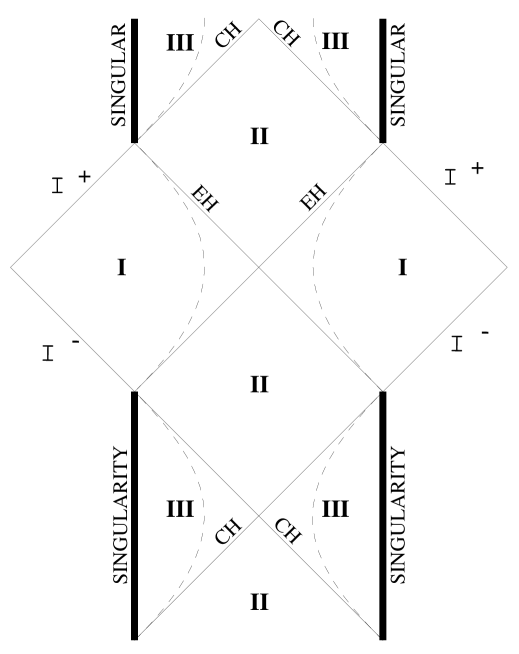
FIG. 1.: Causal structure for the two non-extremal black strings (17) and (56), as well as for the Reissner-Nordstr$\o$m and Horne-Horowitz solutions. The hyperbolae denote the static limits present in our solutions, which do not appear in the previous two cases. Whereas the static limit inside region III is present in both of our two cases, the limit in the asymptotically flat region I is the ergosphere present only in the second solution (56).

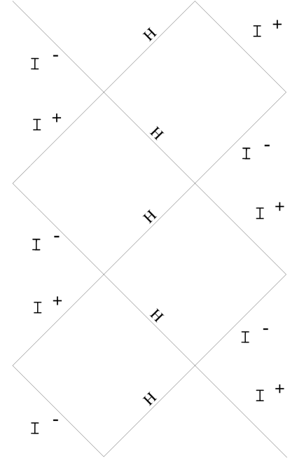
FIG. 2.: Causal structure of the extremal limit of the first family of black strings (17) and the extremal Horne-Horowitz solution.

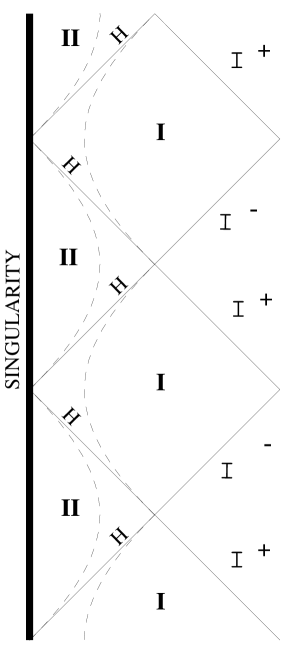
FIG. 3.: Causal structure of the $Q^{2}+4e^{2}=m^{2}$ extremal limit of our second family (56) of black string solutions, as well as of the extremal Reissner-Nordstr$\o$m solution. The hyperbolae here depict the ergosphere (region I) and the inner static limit (region II) present in our case, in contrast to Reissner-Nordstr$\o$m.

- [1] E. Witten, Phys. Rev. D44 (1991) 314; G. Mandal, A.M. Sengupta and S.R. Wadia, Mod. Phys. Lett. A6 (1991) 1685.
- [2] N. Ishibashi, M. Li and A.R. Steif, Phys. Rev. Lett. 67 (1991) 3336;
- [3] J.H. Horne and G.T. Horowitz, Nucl. Phys. B368 (1992) 444.
- [4] M.D. McGuigan, C.R. Nappi and S.A. Yost, Nucl. Phys. B375 (1992) 421; O. Lechtenfeld and C. Nappi, Phys. Lett. B288 (1992) 72.
- [5] M. Banados, C. Teitelboim, and J. Zanelli, Phys. Rev. Lett. 69 (1992) 1849; M. Banados, M. Henneaux, C. Teitelboim and J. Zanelli, Phys. Rev D48 (1993) 1506; D. Cangemi, M. Leblanc and R.B. Mann, Phys. Rev D48 (1993) 3606.
- [6] G.T. Horowitz and D.L. Welch, Phys. Rev. Lett. 71 (1993) 328; N. Kaloper, Phys. Rev. D48 (1993) 2598; A. Ali and A. Kumar, Mod. Phys. Lett. A8 (1993) 2045.
- [7] I.I. Kogan, Mod. Phys. Lett. A7 (1992) 2341; G. Clement, Class. Quant. Grav. 10 (1993) L49; Paris Curie Univ. VI preprint GCR-94-02-01/gr-qc/9402013; Class. Quant. Grav. 11 (1994) L115; K. Shiraishi and T. Maki, Class. Quant. Grav. 11 (1994) 695; Phys. Rev. D49 (1994) 5286; Class. Quant. Grav. 11 (1994) 1687; Class. Quant. Grav. 11 (1994) 2781; G. Lifschytz and M. Ortiz, Phys. Rev. D49 (1994) 1929; A.R. Steif, Phys. Rev. D49 (1994) 585; B. Reznik, Phys. Rev. D45 (1992) 2151; Tel Aviv preprint TAUP-2142-94/gr-qc/9403027; K. Ghoroku and A.L. Larsen, Phys. Lett. B328 (1994) 28; A.L. Larsen and N. Sanchez, Phys. Rev. D50 (1994) 7493.
- [8] T.H. Buscher, Phys. Lett. B94 (1987) 59; Phys. Lett. B201 (1988) 466; A. Giveon, E. Rabinovici and G. Veneziano, Nucl. Phys. B322 (1989) 167; G. Veneziano, Phys. Lett. B265 (1991) 287.
- [9] N. Marcus and J.H. Schwarz, Nucl. Phys. B228 (1983) 145; S. Cecotti, S. Ferrara and L. Girardello, Nucl. Phys. B308 (1988) 436; S.F. Hassan and A. Sen, Nucl. Phys. B375 (1992) 103;
- [10] K.A. Meissner and G. Veneziano, Mod. Phys. Lett. A6 (1991) 3397; Phys. Lett. B267 (1991) 33; M. Gasperini, J. Maharana and G. Veneziano, Phys. Lett. B272 (1991) 277; Phys. Lett. B296 (1992) 51; M. Gasperini and G. Veneziano, Phys. Lett. B277 (1992) 256.
- [11] A. Sen, Phys. Lett. B271 (1991) 295; Phys. Lett. B274 (1992) 34; Nucl. Phys. B404 (1993) 109; Phys. Rev. Lett. 69 (1992) 1006; S.F. Hassan and A. Sen, Nucl. Phys. B405 (1993) 143.
- [12] J. Maharana and J.H. Schwarz, Nucl. Phys. B390 (1993) 3.
- [13] A. Giveon, Mod. Phys. Lett. A6 (1991) 2843; A. Giveon and M. Roček, Nucl. Phys. B380 (1992) 128; E.B. Kiritisis, Mod. Phys. Lett. A6 (1991) 2871; Nucl. Phys. B405 (1993) 109; S.K. Kar, S.P. Khastgir and A. Kumar, Mod. Phys. Lett. A7 (1992) 1545; A. Kumar, Phys. Lett. B293 (1992) 49.
- [14] M. Roček and E. Verlinde, Nucl. Phys. B373 (1992) 630.
- [15] P. Ginsparg and F. Quevedo, Nucl. Phys. B385 (1992) 527; I. Bars and K. Sfetsos, Phys. Rev. D46 (1992) 4495; Phys. Rev. D46 (1992) 4510; Phys. Lett. 301 (1993) 183; K. Sfetsos, Nucl. Phys. B389 (1993) 424.
- [16] A. Tseytlin, Nucl. Phys. 399 (1993) 601; B411 (1994) 509; I. Bars and K. Sfetsos, Phys. Rev. D48 (1993) 844.
- [17] X.C. de la Ossa and F. Quevedo, Nucl. Phys. 403 377; E. Alvarez, L. Alvarez-Gaume, J.L.F. Barbon and Y. Lozano, Nucl. Phys. B415 (1994) 415; E. Alvarez, L. Alvarez-Gaume and Y. Lozano, Phys. Lett. B336 (1994) 183; K. Sfetsos, D50 (1994) 2784; C.P. Burgess, R.C. Myers and F. Quevedo, McGill University preprint MCGILL-94-41, Nov. 1994/hep-th/9411195.
- [18] A. Giveon, M. Porrati and E. Rabinovici, Phys. Rep. 244 (1994) 244.
- [19] I. Bakas, Nucl. Phys. B428 (1994) 374; D.V. Galtsov and O.V. Kechkin, Phys. Rev. D50 (1994) 7394.
- [20] A.A. Tseytlin, Phys. Lett. B317 (1993) 559; S.P. Khastgir and A. Kumar, Bhubaneswar preprint IP-BBSR-93-72/hep-th-9311048; N. Kaloper, Phys. Lett. B336 (1994) 11.
- [21] R. Dijkgraaf, H. Verlinde and E. Verlinde, Nucl. Phys. B371 (1992) 269; I. Bars and K. Sfetsos, Phys. Rev. D46 (1992) 4510; M.J. Perry and E. Teo, Phys. Rev. Lett. 70 (1993) 2669; P. Yi, Phys. Rev. D48 (1993) 2777.
- [22] G.T. Horowitz and A.A. Tseytlin, Imperial College preprint IMPERIAL-TP-93-94-51/hep-th/9408040; Phys. Rev. D50 (1994) 5204.
- [23] D. Gross and J. Sloan, Nucl. Phys. B291 (1987) 41.
- [24] E. Witten, Phys. Lett. B155 (1985) 151.
- [25] S. Deser, R. Jackiw and S. Templeton, Ann. Phys. 140 (1982) 372; Phys. Rev. Lett. 48 (1982) 975.
- [26] N. Kaloper, Phys. Lett. B320 (1994) 16.
- [27] S.W. Hawking and G.F.R. Ellis, “The Large Scale Structure of Space-Time”, Cambridge University Press, 1973, page 165.
- [28] J.H. Horne, G.T. Horowitz and A.R. Steif, Phys. Rev. Lett. 68 (1992) 568.
- [29] D. Garfinkle, Phys. Rev. D46 (1992) 4286; see also D. Garfinkle and T. Vachaspati, Phys. Rev. D42 (1990) 1960.
- [30] S. Weinberg, “Gravitation and Cosmology”, J. Wiley Sons, 1972, page 145.
- [31] J.D. Brown, E. Martinez and J.W. York, Phys. Rev. Lett. 66 (1991) 2281.
- [32] S. Deser, R. Jackiw and G. t’Hooft, Ann. Phys. 152 (1984) 220; S. Deser and R. Jackiw, Ann. Phys. 153 (1984) 405; G. Clement, Int. J. Theor. Phys. 24 (1985) 267.
- [33] R. Kallosh et. al., Phys. Rev. D46 (1992) 5278.