A numerical study of the RG equation for the deformed $O(3)$ nonlinear sigma model

Abstract

The Renormalization Group equation describing the evolution of the metric of the nonlinear sigma model poses some nice mathematical problems involving functional analysis, differential geometry and numerical analysis. In this article we briefly report some results obtained from the numerical study of the solutions in the case of a two dimensional target space (deformation of the $O(3)$ $\sigma$-model). In particular, our analysis shows that the so-called sausages define an attracting manifold in the $U(1)$-symmetric case, at one loop level. Moreover, data from two–loop evolution are used to test the association [1] between the so–called $SSM_{\nu}$ field theory and a certain $U(1)$-symmetric, factorized scattering theory (FST).

I Renormalization Group equation

The perturbative renormalization of the non linear $\sigma$-model [2] gives rise to a deformation of the metric according to the (one–loop) equation

$$\frac{{\rm d}g_{ij}}{{\rm d}t}\>=\>-\frac{1}{4\pi}R_{ij}+O(R^{2})\;.$$ (1)

This second order non linear partial differential equation (PDE) has been studied in the simplest case of 2-dimensional target manifolds in ref. [1]. A whole family of solutions is known for the topology of the sphere $S^{2}$ or for the torus. In this letter we consider the case of $S^{2}$ only, but our method is easily adapted to the toroidal case. As is well known we can introduce local coordinates $\{y,\varphi\}$ in such a way that the metric is conformally flat:

$$g_{ij}\>=\>e^{\phi}\delta_{ij}$$ (2)

and the RG equation valid to all loop reduces to a single non linear PDE,

$$\frac{\partial\phi}{\partial t}\>=\>\beta(R)$$ (3)

where $\beta(R)$ is the exact $\beta-$function and

$$R\>=\>-e^{-\phi}\left[{\partial^{2}\phi\over\partial^{2}y}+{\partial^{2}\phi\over\partial^{2}\varphi}\right]$$ (4)

is the scalar curvature.

A family of solutions in the case of one–loop, namely $\beta(x)=-x/4\pi$ has been presented in [1]. These can be obtained starting from the ansatz

$$\phi(y,\varphi;t)\>=\>-\log[a(t)+b(t)f(y)+c(t)h(\varphi)]\;.$$ (5)

The only solutions of this kind which can be extended to $t\rightarrow-\infty$ (UV limit) without encountering singularities and which exibits a residual $U(1)$ symmetry are the so-called sausage solutions, parametrized by a single real constant $\nu$:

$$\phi(y,t) = -\log(a(t)+b(t)\cosh 2y)$$ (6)

$$a(t) = \frac{1}{2}\nu\coth\left[\frac{\nu}{2\pi}(t_{0}-t)\right]\;,\quad b(t)=\frac{\nu}{2\sinh\left[\frac{\nu}{2\pi}(t_{0}-t)\right]}\;.$$ (7)

These trajectories in the space of all metrics are believed to be the one–loop approximation of some integrable deformation of the costant–curvature trajectory ($O(3)$ $\sigma$-model), to which they tend as $\nu\rightarrow 0$. To discuss the general solution of the RG equation we have to construct a numerical integration algorithm. The first problem is posed by the divergence of the conformal factor as $|y|\rightarrow\infty$: $\phi\sim-2|y|$ as $|y|\rightarrow\infty$. This general property (which follows directly from Gauss–Bonnet theorem) causes the factor $\exp(-\phi)$ to diverge, hence amplifying the numerical error of the differential term at large $|y|$. To overcome this difficulty we introduce a background field $\phi_{0}(y,t)$, and we consider the equation for the shifted field $\phi=\eta+\phi_{0}$. The background field is conveniently chosen as the constant curvature solution

$$\phi_{0}\>=\>\log\left[{A(t)}\over{4\pi\cosh^{2}y}\right]\;,$$ (8)

where according to the RG equation $A(t)$ satisfies

$$\dot{A}(t)A(t)^{-1}\>=\>\beta(8\pi A(t)^{-1})\;.$$ (9)

Introducing a new evolution parameter (“time”) $\tau$, defined by

$$A(t)\>=\>4\pi e^{-\tau}$$ (10)

the RG equation expressed in terms of the shifted field $\eta$ reads

$$\partial_{\tau}\eta\>=\>1-\frac{\beta(\tilde{R}(\eta))}{\beta(2e^{\tau})}\\$$ (11)

with

$$\tilde{R}(\eta)\equiv R(\phi_{0}+\eta)\>=\>e^{\tau-\eta}(2-\Delta_{0}\eta)\;.$$ (12)

Here $\Delta_{0}\equiv\cosh^{2}\!y\,\partial^{2}_{y}+\partial^{2}_{\varphi}$ is the standard $O(3)-$invariant Laplacean on the sphere. The original time scale can be simply recovered by quadratures

$$t_{0}-t\>=\>\int^{\tau}_{0}\frac{{\rm d}\tau^{\prime}}{\beta(2e^{\tau^{\prime}})}\;.$$ (13)

At this stage we restrict our attention to $U(1)-$symmetric solutions $\eta=\eta(y,t)$.

II Numerical integration of the RG equation

At this point it is convenient to adopt the standard spherical coordinates by letting $y=\log(\cot(\vartheta/2))$. To get a good accuracy in the evaluation of the Laplacean we apply the spectral method, that is we expand $\eta$ in Legendre polynomials $P_{n}(\cos\vartheta)$, which are the eigenfunctions of $\Delta_{0}$. Thus, we developed the following finite–dimensional implementation of the standard expansion in Legendre polynomials.

Let $x_{j}^{(L)}$ be the zeroes of the $L$-th Legendre polynomial $P_{L}(x)$; we adopt $\{x_{j}^{(L)}\>|\>j=1,\dots,L\}$ as our finite grid and sample the field $\eta(y,t)$ at the image points $y^{(L)}_{j}$.
The finite Legendre expansion is then realized as follows:

$$\eta(x)\>=\>\sum_{l=0}^{\infty}\eta_{l}P_{l}(x)\approx\sum_{l=0}^{L-1}\eta_{l}P_{l}(x)$$ (14)

$$\eta_{l}=\frac{1}{2}\int^{1}_{-1}{\rm d}x\;\eta(x)P_{l}(x)(2l+1)\approx\frac{1}{2}\sum_{j=1}^{L}\eta(x_{j}^{(L)})P_{l}(x_{j}^{(L)})w_{j}^{(L)}(2l+1)\equiv(\cal L\eta)_{l}$$ (15)

where $w_{j}^{(L)}$ are the Gaussian integration weights [5] for Legendre polynomials. This finite expansion allows us to represent the Laplacean exactly on polynomials of degree less than $L$, since the coefficients $\eta_{l}$ are exact in this case. The lack of a fast implementation analogous to FFT limits our algorithm in practice to $L\sim 200$ on current workstations, but this proves to be adequate for our purposes.

Having determined the finite transform $\cal L$ on the basis of Legendre polynomials, the action of the Laplacean $\Delta_{0}$ is represented by a matrix $\cal L^{-1}\Lambda\cal L$, where $\Lambda$ is diagonal, with eigenvalues $\{-l(l+1)\>|\>l=0,\dots,L-1\}$. In terms of this representation is quite easy to compute the spectrum of zero–modes of the field $\phi$, a problem considered in ref. [1]. We just have to diagonalize the finite matrix $-(1/2)\Delta+(1/8)\tilde{R}$, where $\Delta=\exp(\tau-\eta)\Delta_{0}$. The results agree with the previously computed ones for the sausages [7] (notice however that the present method is much simpler and the spectrum can be computed in parallel with the RG evolution).

With the finite Legendre–transform algorithm at hand, we can now consider the integration of eq. (11). We can work to any loop, provided we know the corresponding $\beta-$function. We have implemented the algorithm in matlab [6] which provides efficient routines of dia -go -nalization and of adaptive-step integration. The accuracy of the code has been tested on the known one–loop sausage solution, attaining a typical maximal deviation of $1$ part in $10^{9}$ over a time interval $-3<\tau<2$ and $\nu<.25$. In Fig.1 we show a typical one–loop sausage evolution; to aid the visualization we have recovered the embedding of the surface in $R^{3}$ in such a way that the induced metric coincides with $\exp(\phi)\delta_{ij}$. The accuracy is limited essentially from the large eigenvalues of the Laplacean which grow as the square of the finite grid dimension. Moreover as $\nu$ and/or $-\tau$ increase the curvature tends to be confined at the extremities of the sausage, which requires finer and finer grid. Presently, up to $200$ points, we cannot go beyond $\tau\approx-4$ for $\nu\approx.25$, but there is no limit in principle.

The algorithm can now be applied to investigate, at one–loop, the existence of attracting manifolds, in the space of all metrics. A conjecture of Fateev and Zamolodchikov states that the sausages constitute a stable manifold and all other geometries converge to some sausage, parametrized by the real $\nu$, in the IR direction $\tau\rightarrow\infty$.
This fact manifests itself quite clearly in our numerical data. We may define a distance function by

$$\mathrm{dist}(\eta_{1},\eta_{2})\>=\>\int{\rm d}x[\tilde{R}(\eta_{1})-\tilde{R}(\eta_{2})]^{2}$$ (16)

and measure the distance to the sausage hypersurface by

$$D(\tau)\>=\>\inf_{\nu}{\mathrm{dist}}(\eta(\tau),\eta_{\nu}(\tau))$$ (17)

where $\eta_{\nu}$ is the sausage solution specified by $\nu$. The data show a clear exponential decay $D(\tau)\approx A\exp(-m\tau)$, with $m\approx 8$ regardless of the initial surface (see Tab.1). For any given starting geometry we record the value $\nu_{\mathrm{eff}}$ where the infimum is reached; its limit $\nu_{\mathrm{lim}}$ as $\tau\rightarrow\infty$ gives a definition of sausageness of any given surface. For instance, given an ellipsoid with cylindrical symmetry and eccentricity $\epsilon$ we can measure $\epsilon(\nu_{\mathrm{lim}})$, at one–loop order (see Fig.2). This shows a remarkable property: $\epsilon$ is a universal function of $s=\nu_{\mathrm{lim}}\frac{e^{-\bar{\tau}}}{2}$, where $\bar{\tau}$ is the starting scale of the evolution. This function seems to be $\epsilon=\tanh s$, at least for small $s$.

III Variational equations and stability

Another way to discuss the attracting nature of the sausage manifold is to study the Jacobi variational equations around the sausage solution. The linearized equations take on the following form ( calling $\chi$ the variation):

$$\partial_{\tau}\chi\>=\>H(\eta,\tau)\chi$$ (18)

where

$$H(\eta,\tau)\>=\>\frac{\beta^{\prime}(\tilde{R}(\eta))}{\beta(2e^{\tau})}\left(e^{\tau-\eta}\Delta_{0}+\tilde{R}(\eta)\right)\;.$$ (19)

The spectrum of $H$ is not a priori of much significance, since the evolution equations are time–dependent. However, if we rely on the adiabatic approximation, the spectrum is directly related to stability. Applying the finite Legendre–transform $\cal L$ the spectrum of $H$ is easily reduced to that of a Hermitean matrix; choosing for $\eta$ some sausage $\eta_{\nu}$ we find a single positive eigenvalue denoting an unstable mode. As we presently show, this is easily interpreted.
It is immediate to find that the Jacobi variational equation at one loop:

$$\partial_{\tau}\chi\>=\>\frac{1}{2}\left(\exp(-\eta_{\nu})\Delta_{0}+e^{-\tau}\tilde{R}(\eta_{\nu})\right)\chi$$ (20)

admits the two solutions

$$\chi_{1}\>=\>\tilde{R}(\eta_{\nu})$$ (21)

$$\chi_{2}\>=\>1-(1/2)\exp(-\tau)\tilde{R}(\eta_{\nu})\;.$$ (22)

Their existence is not surprising: the family of sausage solutions (6) depends on two parameters $t_{0}$ and $\nu$, so that the derivatives with respect to $t_{0}$ and $\nu$ give rise to two independent solutions of the variational equations. Now $\chi_{1}$, which comes from the time derivative represents the unstable solution; this kind of instability is of no concern, since it corresponds to a simple redefinition of the initial time parameter $t_{0}$ and it can be fixed by restricting to a given initial area. The other solution $\chi_{2}$ comes from the $\nu-$derivative and is tangent to the manifold of sausages. The component of a generic variation $\chi$ which is orthogonal to both $\chi_{1}$ and $\chi_{2}$ provides a measure of the distance of a generic solution from the sausage manifold.

Numerical results (Tab.2 and 3) show that the orthogonal part is exponentially decreasing with a slope ($\approx 8.73$) much higher than the slope of $\chi_{2}$, which from equation (22) is found to be 2. The point is that there is an overall convergence in the infrared toward the constant curvature metric. All sausages converge to a sphere with vanishing radius, forcing the decay of the mode $\chi_{2}$; however, the rate of this convergence is slower than the rate of decay of all other modes. Fig.3 shows how the longitudinal component (plotted in the vertical direction) is stil large when the transversal one is already negligible. In Fig.4 there is an impressive, though only qualitative proof of what we found (one should compare Fig.4 with Fig.1, where the sausage evolution is plotted).

Conversely, the evolution in the ultraviolet direction $\tau\rightarrow-\infty$ is strongly unstable, which makes it quite hard to follow numerically; all truncation errors are chaotically amplified and the calculation becomes rapidly unreliable.

IV The free energy of the sausage sigma model

In ref. [1] the model corresponding to $U(1)-$symmetric, one–loop deformation of the $O(3)$ sigma model (termed $SSM_{\nu}$ model) is associated with a $U(1)-$symmetric deformation of the $O(3)$ FST. To test the correctness of the identification, some physical quantities calculated from $S$-matrix data via Thermodynamic Bethe Ansatz tecniques are compared in the UV region with the corresponding quantities obtained perturbatively from the one–loop sausage action

$$\cal A_{SSM_{\nu}}\;=\;\int d^{2}x\frac{(\partial_{\mu}y)^{2}\>+\>(\partial_{\mu}\varphi)^{2}}{a\>+\>b\cosh 2y}\;{}.$$ (23)

Their non–trivial matching is a strong (though indirect) proof of the correctness of the association.

However, while for the FST we have exact (at least in principle) results, for the field theory we are strongly limited by the fact that the “sausage metric” is a solution to the RG equation only to one–loop. So, it would be very important to have higher–loop solutions of the RG equation with the same features of the sausage, so to confirm (or deny) the validity of the association proposed in [1]. This is not to be taken for granted. To any relativistic FST one would like to associate an integrable QFT; however, even if one assumes that the action (23) is the one–loop approximation of an exact trajectory of the RG group, which would define the exact sausage model, there is no a prori reason to expect such model to be integrable. In particular, $S^{2}$ with any $U(1)$-symmetric metric is not a symmetric space and one cannot use the results of refs. [3][4] to establish the classical and/or quantum integrability of the model.

Considering the zero–temperature free energy $f(A)$ in the presence of a constant external field $A$, the one–loop calculation based on the action (23) gives the result [1]

$$f(A)=-A^{2}\>e^{\phi(y=0,t)}\;,$$ (24)

where $t_{0}-t=\log A/\Lambda$, $\Lambda$ is a subtraction scale and one works in the “scaling limit”:

$$\nu\rightarrow 0\;,\quad t\rightarrow-\infty\;,\quad\nu t\;\;\mathrm{fixed}$$ (25)

This limit serves to eliminate all higher–loops contributions, which cannot be properly taken into account using the one–loop action (23). To obtain higher–loop correction to (24) one needs the corresponding higher–loop solution of the RG equation. Formula (24) however remains valid, assuming as natural that the higher–loop action is an even, convex function of $A$.

With our algorithm, the quantity in (24) is evaluated as

$$f(A)_{\mathrm{num}}=-A^{2}e^{\eta(t,x_{\mathrm{med}})}e^{\phi_{0}(t,y=0)}=-A^{2}e^{\eta(t,x_{\mathrm{med}})}\frac{t_{0}-t}{4\pi}$$ (26)

where $x_{\mathrm{med}}$ is the middle point of the finite grid with represents the coordinate $x=\cos\theta$. The two–loop $\beta-$function is well known [2]: $\beta(x)=-x/4\pi-x^{2}/(4\pi)^{2}$. Lacking an exact, $U(1)-$symmetric two–loop solution of the RG equation, the first thing one could try is a linerization around the one–loop sausage solution, regarding $\nu$ as perturbative parameter. Notice in fact that $\nu$ may be scaled out from the sausage solution, through the substitutions

$$\phi\rightarrow\phi+\log\frac{\nu}{4\pi}\;,\quad t\rightarrow\nu t$$ (27)

which leave the one–loop equation invariant (actually, with our choice, the scalar curvature $R$ is conveniently scaled by a factor of $4\pi$). On the other hand the two–loop equation is transformed by (27) to

$$\frac{\partial\phi}{\partial t}\>=\>-R-\nu R^{2}$$ (28)

where the last term could now be treated perturbatively for small sausage deformations. However, even the linearized equation proves to be too difficult to solve exactly, when the correct boundary conditions for $\phi$ are taken into account, and we resort to a numerical approach.

Our idea is the following: in the scaling limit (far UV and small deformations), the exact solution must have the same features of its various loop–wise approximations. We can now study with our algorithm the two–loop evolution, using as initial data in the far UV (say at $t=\bar{t}$) a metric with the “sausage features ” (e.g. a sausage itself, one–loop solution). We then evaluate our physical quantity in a fixed scale interval $(t_{1},t_{2})$ and we compare it with the same quantity evaluated starting from the FST by means of Bethe Ansatz techniques [1][8]. We expect that the difference between the two quantities tends to zero when the starting scale of the evolution is pushed farther and farther in the UV. At one–loop level this is easily verified, using as starting data, e.g., the function

$$\phi(\bar{t},y)=\phi_{0}(\bar{t},y)+\log\frac{2}{\nu}-\log(1+2e^{\nu(\bar{t}-t_{0})/2\pi}\cosh 2y+e^{\nu(\bar{t}-t_{0})/\pi})$$ (29)

The above mentioned difference vanish exponentially when the initial scale $\bar{t}$ is sent to $-\infty$.

In ref. [1] the Bethe Ansatz techniques are used to compute the free energy as a function of the chemical potential $h$ coupled to the physical particles. The input is the factorized, $U(1)-$symmetric $S$-matrix with deformation parameter $\lambda$ relative to the $S$-matrix of the $O(3)$ sigma model. The output reads, in the scaling limit $\lambda\to 0$, $h\to\infty$, $\lambda\log h$ fixed,

$$f(h)=-\frac{h^{2}}{2\pi\lambda}\frac{1-u}{1+u}\left[1+4\lambda\frac{u}{1-u^{2}}\log\frac{1-u}{2\lambda}+O(\lambda^{2}\log^{2}\lambda)\right]$$ (30)

where $u=\left(\frac{me^{3/2}}{8h}\right)^{2\lambda/(1-\lambda)}$, and $m$ is the mass of the physical particles. The connection among the various quantities in (30) and those contained in the perturbative expressions is established as follows:

$$\frac{me^{3/2}}{8}=\Lambda+O(\nu)$$ (31)

$$h=A+O(\nu)$$ (32)

$$\frac{\lambda}{\nu}=\frac{1}{4\pi}[1+O(\nu)]$$ (33)

The relation between the “scale variables” $z=\nu(t_{0}-t)/2\pi$ and $u$ follows by noticing that in the perturbative calculations we put $t_{0}-t=\log(A/\Lambda)$. Substituting (31)-(33) in (30) we obtain

$$\frac{f(A)_{\mathrm{an}}}{A^{2}}=-\frac{1}{\pi}\left[\frac{2\pi}{\nu}\tanh(z/2)+\frac{\log\nu}{\cosh^{2}(z/2)}-\frac{\log(2\pi(1-e^{-z}))}{\cosh^{2}(z/2)}+O(\nu)\right]$$ (34)

where the subscript “an” stands for “analytical” (compare (26)). The first term comes from the one–loop action (23), while the second and the third represent the two–loop contributions. The presence of the non–analytic behaviour $\nu\log\nu$ ensures the correct $O(3)-$symmetric limit ($\nu\to 0$ at fixed $t_{0}-t$). Corrections of order $\nu$ are not known; to establish them we should know the corrections of the same order to eqs. (31)-(33). Our aim is now to compare expressions $f(A)_{\mathrm{an}}$ and $f(A)_{\mathrm{num}}$.

We have collected numerical data relative to the two–loop evolution of sausages with $\nu$ fixed, starting at different initial scales $\bar{\tau}$ (recall that $\tau$ is related to $t_{0}-t$ by (13)). Fig. 5 reports the results; here $\nu=0.1$ and the $\tau$ interval is chosen as $(\tau_{1}=-3.85,\tau_{2}=-3.8)$. The quantity $\Delta$ is defined as

$$\Delta(\bar{\tau})=\max_{\tau_{1}<\tau<\tau_{2}}\,|f(A)_{\mathrm{an}}/A^{2}-f(A)_{\mathrm{num}}/A^{2}|$$ (35)

and it is plotted for different values of the initial scale $\bar{\tau}$.
$\Delta$ does not decrease when the scale is pushed towards far UV; instead, initially increase and then reach an asymptotical value. The value to which $\Delta$ tends is of order $10^{-2}$; that means a discrepancy of about 5 parts in 10000 relative to the value of the free energy. This is well above the numerical errors of our algorithm.
We controlled if this discrepancy can be reabsorbed in a “renormalization” of $\nu$; leaving it as a free parameter in (34), we seeked for a minimum of $\Delta$ in a neighborhood of $0.1$. The result was negative.
In principle, the non–zero asymptotic value of $\Delta$ may be eliminated by the $O(\nu)$ correction; to test this hypotesis we repeated the evaluation of $\Delta$ for different $\nu$ values, and correspondingly redefined the $\tau-$interval so to leave the interval $(\nu t_{1},\nu t_{2})$ fixed, according to the scaling limit. The results are summarized in Fig. 6: the asymptotic value of $\Delta$ seems not to depend appreciably upon $\nu$. It remains always of the same order of magnitude, and does not grow with $\nu$.

V Conclusions

The RG equation for the non linear sigma model with fields taking values on a target space with the topology of the 2-sphere is a nonlinear partial–differential equation, possibly nonlocal (if the $\beta$ function were known to all loop). These features makes it hard to caracterize the general solution in an analytical way. The numerical approach appears at the moment to be the only way to obtain quantitative informations about the higher–loop solutions.
The spectral method presented in this letter proved to be a useful tool for the construction of an efficent algorithm; this remains true even if the exact RG equation should turn out to be nonlocal. Another future developement concerns the study of solutions without any residual symmetry, hopefully with the help of some “fast” algorithm analogous to the well known FFT for the Fourier case.

In the one–loop approximation we have shown the attractive nature of the $U(1)-$symmetric family of solutions, the so–called sausages.

As far as the two–loop evolution is concerned, however, our data show a discrepancy between calculations based on the RG equation and analogous calculations based on the $U(1)-$symmetric FST proposed in [1].
This probably means that the identification put forward in [1] is not correct, in the sense that the $U(1)-$symmetric FST after all does not correspond to a $U(1)-$symmetric nonlinear sigma model reducing to the sausage at one–loop. On this point, the following alternative conjecture seems natural.

The factorized $S-$matrix put forward in [1] is a quantum–group deformation of the $O(3)$ $S-$matrix, in the sense of, e.g., ref. [9]. In practice, the triplet of massive particles of the model forms a spin-one irreducible representation of $SU(2)_{q}$ and scatter through a $SU(2)_{q}-$invariant $S-$matrix with $q\simeq e^{i\lambda}$. Hence, the QFT corresponding to such FST should enjoy a nonlocal hidden $SU(2)_{q}$ invariance, whose $U(1)$ subgroup coincides with the manifest $U(1)-$symmetry locally implemented. In the usual spirit of the sigma models, in which the field–theoretical symmetries follow from geometrical properties of the target manifold, we expect this quantum–group invariance to follow from the noncommutative geometry of a $q-$deformed target manifold $SU(2)_{q}/U(1)$ (attempts in constructing $q-$deformed sigma models can be found in refs. [10] [11]). In other words, we suspect that the FST put forward in [1] does not correspond, beyond the one–loop approximation, to any conventional nonlinear sigma model (that is to a model in which the fields take values in an ordinary manifold with commuting geometry). It would be interesting to explain why there exist a one–loop conventional sigma model, perhaps through a suitable expansion near $q=1$. This matter clearly requires further investigations.

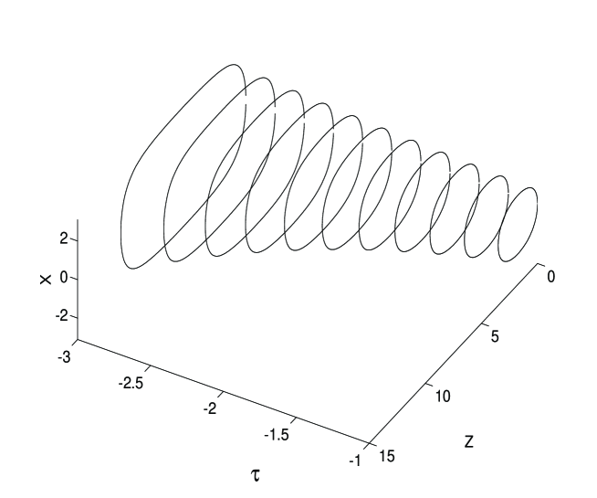
FIG. 1.: One–loop evolution of the sausage solution

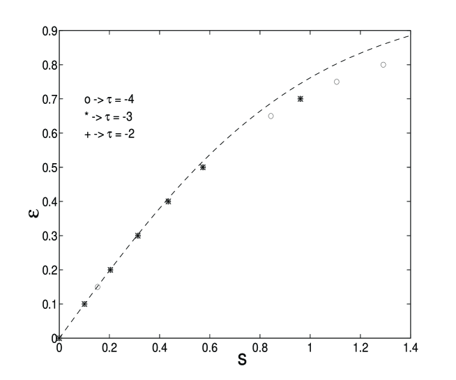
FIG. 2.: The eccentricity as a universal function of $s=\nu_{\mathrm{lim}}\frac{e^{-\bar{\tau}}}{2}$. The dashed curve is $\epsilon=\tanh s$

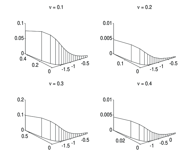
FIG. 3.: Three–dimensional view of the decay of the longitudinal and transversal modes

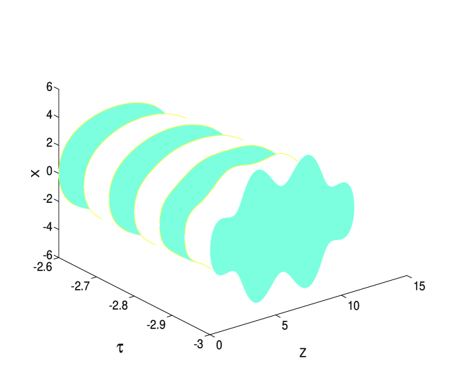
FIG. 4.: A pictorial way of illustrating the attractive nature of the sausage solution

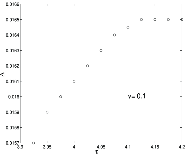
FIG. 5.: The difference, for various values of $\bar{\tau}$, between the free energy evaluated from RG equation and the corresponding quantity evaluated from FST data

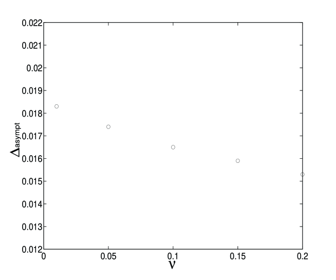
FIG. 6.: The asymptotic value of $\Delta$ for different values of the parameter $\nu$

TABLE I.: Evolution of an ellipsoid; $D$ is the distance to the sausage manifold.

$\tau$	$\nu_{\mathrm{eff}}$	$D$
-4.00000	0.03761	0.04265
-3.90000	0.03609	0.01453
-3.80000	0.03557	0.00551
-3.70000	0.03536	0.00217
-3.60000	0.03528	0.00088
-3.50000	0.03524	0.00056
-3.40000	0.03523	0.00015
-3.30000	0.03522	0.00006
-3.20000	0.03522	0.00003
-3.10000	0.03522	0.00001
-3.00000	0.03521	0.00000
-2.90000	0.03521	0.00000
-2.80000	0.03521	0.00000
-2.70000	0.03521	0.00000
-2.60000	0.03521	0.00000
-2.50000	0.03521	0.00000

TABLE II.: Decay of longitudinal component ($\chi_{\parallel}$) and of the transversal one ($\chi_{\perp}$) at $\nu=.1$

$\tau$	$\chi_{\parallel}$	$\chi_{\perp}$
-1.9000	0.0047	0.1772
-1.8000	0.0055	0.0734
-1.7000	0.0051	0.0303
-1.6000	0.0043	0.0125
-1.5000	0.0036	0.0051
-1.4000	0.0030	0.0021
-1.3000	0.0025	0.0009
-1.2000	0.0020	0.0004
-1.1000	0.0017	0.0001
-1.0000	0.0014	0.0001
-0.9000	0.0011	0.0000
-0.8000	0.0009	0.0000
-0.7000	0.0008	0.0000
-0.6000	0.0006	0.0000
-0.5000	0.0005	0.0000

TABLE III.: Decay of longitudinal component ($\chi_{\parallel}$) and of the transversal one ($\chi_{\perp}$) at $\nu=.3$

$\tau$	$\chi_{\parallel}$	$\chi_{\perp}$
-1.9000	0.0761	0.4415
-1.8000	0.0963	0.2057
-1.7000	0.0944	0.0939
-1.6000	0.0848	0.0421
-1.5000	0.0734	0.0186
-1.4000	0.0623	0.0081
-1.3000	0.0524	0.0035
-1.2000	0.0438	0.0015
-1.1000	0.0364	0.0006
-1.0000	0.0302	0.0003
-0.9000	0.0250	0.0001
-0.8000	0.0207	0.0000
-0.7000	0.0171	0.0000
-0.6000	0.0140	0.0000
-0.5000	0.0116	0.0000

REFERENCES

- [1] V.A. Fateev, E. Onofri and Al.B. Zamolodchikov, Nucl. Phys. B406 (1993) 521
- [2] D. Friedan, Ann. Phys. 163 (1985) 318
- [3] H. Eichenerr, M. Forger, Nucl. Phys. B155 (1979) 381; B164 (1980) 528; Commun. Math. Phys. 82 (1981) 227
-
[4]
A.M. Polyakov, Phys. Lett. 72B (1977) 224
D. Spector, Phys. Lett. 171B (1986) 231
M. Lüscher, Nucl. Phys. B135 (1978) 1 - [5] H. Hochstadt, The functions of Mathematical Physics, Wiley-Interscience, New York (1971)
- [6] for details about the codes, see L. Belardinelli and E. Onofri, preprint hep-th 9404082 (1994)
- [7] R. Brunelli and G.T. Tecchiolli, ”Stochastic minimization with adaptive memory”, J. Comp. Appl. Math., in press
-
[8]
P. Hasenfratz, M. Maggiore, F. Niedermayer, Phys. Lett.
245B (1990) 522
P. Hasenfratz, F. Niedermayer, Phys. Lett. 245B (1990) 529 - [9] M. Jimbo, Int. J. Mod. Phys. A4 (1989) 3759
-
[10]
I.Y. Arefeva, I.V. Volovich, Mod. Phys. Lett. 6A
(1991) 893
I.Y. Arefeva, I.V. Volovich, Phys. Lett. 264B (1991) 62 - [11] Y. Frishman, J. Lukierski, W.J. Zakrzewski, J. Phys. A26 (1993) 301