Exact solution and interfacial tension of the six-vertex model with anti-periodic boundary conditions

Abstract

We consider the six-vertex model with anti-periodic boundary conditions across a finite strip. The row-to-row transfer matrix is diagonalised by the ‘commuting transfer matrices’ method. From the exact solution we obtain an independent derivation of the interfacial tension of the six-vertex model in the anti-ferroelectric phase. The nature of the corresponding integrable boundary condition on the $XXZ$ spin chain is also discussed.

Short Title: The anti-periodic six-vertex model

ANU preprint MRR 012-95, hep-th/9502040

1 Introduction and main results

The six-vertex model and related spin-$\frac{1}{2}$ $XXZ$ chain play a central role in the theory of exactly solved lattice models [1]. Typically the six-vertex model is ‘solved’ by diagonalising the row-to-row transfer matrix with periodic boundary conditions. Several methods have evolved for doing this, including the co-ordinate Bethe ansatz [1, 2], the algebraic Bethe ansatz [3, 4], and the analytic ansatz [5]. All of these methods rely heavily on the conservation of arrow flux from row to row of the lattice.

In terms of the vertex weights (see figure 1)

$$a=\rho\,\sinh\mbox{\small$\frac{1}{2}$}(\lambda-v),\quad b=\rho\,\sinh\mbox{\small$\frac{1}{2}$}(\lambda+v),\quad c=\rho\,\sinh\lambda$$ (1.1)

the transfer matrix eigenvalues on a strip of width $N$ are given by [1]

$$\Lambda(v)q(v)=\phi(\lambda-v)q(v+2\lambda^{\prime})+\phi(\lambda+v)q(v-2\lambda^{\prime})$$ (1.2)

where

$$\lambda^{\prime} = \lambda-{\rm i}\pi$$ (1.3)

$$\phi(v) = \rho^{N}\sinh^{N}(\mbox{\small$\frac{1}{2}$}v)$$ (1.4)

$$q(v) = \prod_{k=1}^{n}\sinh\mbox{\small$\frac{1}{2}$}(v-v_{k}).$$ (1.5)

The Bethe ansatz equations follow from (1.2) as

$${\phi(\lambda-v_{j})\over\phi(\lambda+v_{j})}=-{q(v_{j}-2\lambda^{\prime})\over q(v_{j}+2\lambda^{\prime})},\quad j=1,\ldots,n.$$ (1.6)

The integer $n$ labels the sectors of the transfer matrix.

Here we consider the same six-vertex model with anti-periodic boundary conditions. That such boundary conditions should preserve integrability is known through the existence of commuting transfer matrices [6]. However, the solution itself has not been found previously. In section 2 we solve the anti-periodic six-vertex model by the ‘commuting transfer matrices’ method [1]. This approach has its origin in the solution of the more general 8-vertex model [7], which like the present problem, no longer enjoys arrow conservation. We find the transfer matrix eigenvalues to be given by

$$\Lambda(v)q(v)=\phi(\lambda-v)q(v+2\lambda^{\prime})-\phi(\lambda+v)q(v-2\lambda^{\prime})$$ (1.7)

where now

$$q(v)=\prod_{k=1}^{N}\sinh\mbox{\small$\frac{1}{4}$}(v-v_{k}).$$ (1.8)

In this case the Bethe ansatz equations are

$${\phi(\lambda-v_{j})\over\phi(\lambda+v_{j})}={q(v_{j}-2\lambda^{\prime})\over q(v_{j}+2\lambda^{\prime})},\quad j=1,\ldots,N.$$ (1.9)

In contrast with the periodic case the number of roots is fixed at $N$.

In section 3 we use this solution to derive the interfacial tension $s$ of the six-vertex model in the anti-ferroelectric regime. Defining $x={\rm e}^{-\lambda}$, our final result is

$${\rm e}^{-s/k_{B}T}=2x^{1\over 2}\prod_{m=1}^{\infty}\left({1+x^{4m}\over 1+x^{4m-2}}\right)^{2}$$ (1.10)

in agreement with the result obtained from the asymptotic degeneracy of the two largest eigenvalues [1, 8].

With anti-periodic boundary conditions on the vertex model, the related $XXZ$ Hamiltonian is

$${\cal H}=\sum_{j=1}^{N}\left(\sigma_{j}^{x}\sigma_{j+1}^{x}+\sigma_{j}^{y}\sigma_{j+1}^{y}+\cosh\!\lambda\,\,\sigma_{j}^{z}\sigma_{j+1}^{z}\right)$$ (1.11)

where $\sigma^{x},\sigma^{y}$ and $\sigma^{z}$ are the usual Pauli matrices, with boundary conditions

$$\sigma_{N+1}^{x}=\sigma_{1}^{x},\quad\sigma_{N+1}^{y}=-\sigma_{1}^{y},\quad\sigma_{N+1}^{z}=-\sigma_{1}^{z}.$$ (1.12)

This boundary condition has appeared previously and is amongst the class of toroidal boundary conditions for which the operator content of the $XXZ$ chain has been determined by finite-size studies [9]. It is thus an integrable boundary condition, with the eigenvalues of the Hamiltonian following from (1.7) in the usual way [1], with result

$$E=N\cosh\!\lambda\,-\sum_{j=1}^{N}{2\cosh\frac{1}{2}\lambda\,\sinh\lambda\over\sinh\frac{1}{2}v_{j}+\sinh\frac{1}{2}\lambda}.$$ (1.13)

We anticipate that the approach adopted here may also be successful in solving other models without arrow conservation. The solution given here can be extended, for example, to the spin-$S$ generalisation of the six-vertex model/$XXZ$ chain [10].

2 Exact solution

To obtain the result (1.7) we adapt where appropriate the derivation of the periodic result (1.2) (specifically, we refer the reader to Ch. 9 of Ref. [1]). We depict a vertex and its corresponding Boltzmann weight graphically, as

$$w(\mu,\alpha|\beta,\mu^{\prime})=\hskip 14.45486pt\rule[-20.23683pt]{0.0pt}{40.47366pt}\begin{picture}(4.0,4.0)(0.0,-0.3)\put(2.0,-2.1){\line(0,1){4.0}} \put(4.0,0.0){\line(-1,0){4.0}} \put(2.0,-3.2){\makebox(0.0,0.0)[b]{\scriptsize\mbox{$\alpha$}}} \put(4.4,0.0){\makebox(0.0,0.0)[l]{\scriptsize\mbox{$\mu^{\prime}$}}} \put(2.0,2.5){\makebox(0.0,0.0)[b]{\scriptsize\mbox{$\beta$}}} \put(-0.4,0.0){\makebox(0.0,0.0)[r]{\scriptsize\mbox{$\mu$}}} \end{picture}$$

where the bond ‘spins’ $\mu,\alpha,\beta,\mu^{\prime}$ are each $+1$ if the corresponding arrow points up or to the right and $-1$ if the arrow points down or to the left. Thus in terms of the parametrisation (1.1) the nonzero vertex weights are

$$w(+,+|+,+)=w(-,-|,-,-)=a$$

$$w(+,-|-,+)=w(-,+|,+,-)=b$$ (2.1)

$$w(+,-|+,-)=w(-,+|,-,+)=c$$

The row-to-row transfer matrix $T$ has elements

$$\rule[-20.23683pt]{0.0pt}{40.47366pt}T_{\mbox{\boldmath$\alpha\beta$}}=\sum_{\mu_{1}}\ldots\sum_{\mu_{N}}\quad\,\,\begin{picture}(12.0,4.0)(0.0,-0.3)\put(2.0,-2.1){\line(0,1){4.0}} \put(5.0,-2.1){\line(0,1){4.0}} \put(7.0,0.0){\line(-1,0){7.0}} \put(7.6,0.0){\line(-1,0){0.2}} \put(8.2,0.0){\line(-1,0){0.2}} \put(8.8,0.0){\line(-1,0){0.2}} \put(9.2,0.0){\line(1,0){4.0}} \put(11.2,-2.1){\line(0,1){4.0}} \put(2.0,-3.2){\makebox(0.0,0.0)[b]{\scriptsize\mbox{$\alpha_{1}$}}} \put(2.0,2.5){\makebox(0.0,0.0)[b]{\scriptsize\mbox{$\beta_{1}$}}} \put(5.0,-3.2){\makebox(0.0,0.0)[b]{\scriptsize\mbox{$\alpha_{2}$}}} \put(5.0,2.5){\makebox(0.0,0.0)[b]{\scriptsize\mbox{$\beta_{2}$}}} \put(3.0,-1.0){\makebox(0.0,0.0)[l]{\scriptsize\mbox{$\mu_{2}$}}} \put(-0.4,0.0){\makebox(0.0,0.0)[r]{\scriptsize\mbox{$\mu_{1}$}}} \put(9.0,-1.0){\makebox(0.0,0.0)[l]{\scriptsize\mbox{$\mu_{N}$}}} \put(13.6,0.0){\makebox(0.0,0.0)[l]{\scriptsize\mbox{$\mu_{N+1}$}}} \put(11.2,-3.2){\makebox(0.0,0.0)[b]{\scriptsize\mbox{$\alpha_{N}$}}} \put(11.2,2.5){\makebox(0.0,0.0)[b]{\scriptsize\mbox{$\beta_{N}$}}} \end{picture}$$ (2.2)

where $\mbox{\boldmath$\alpha$}=\{\alpha_{1},\ldots,\alpha_{N}\}$, $\mbox{\boldmath$\beta$}=\{\beta_{1},\ldots,\beta_{N}\}$, and the anti-periodic boundary condition is such that $\mu_{N+1}=-\mu_{1}$. Now consider an eigenvector $y$ of the form

$$y=g_{1}\otimes g_{2}\otimes\cdots\otimes g_{N}$$ (2.3)

where $g_{i}(\alpha_{i})$ are two-dimensional vectors. From (2.2) the product $Ty$ can be written as

$$\left(Ty\right)_{\mbox{\boldmath$\alpha$}}={\rm Tr}\left[G_{1}(\alpha_{1})G_{2}(\alpha_{2})\cdots G_{N}(\alpha_{N})S\right]$$ (2.4)

where $G_{i}(\pm)$ are $2\times 2$ matrices with elements

$$G_{i}(\alpha)_{\mu\mu^{\prime}}=\sum_{\beta}\hskip 14.45486pt\rule[-20.23683pt]{0.0pt}{40.47366pt}\begin{picture}(4.0,4.0)(0.0,-0.3)\put(2.0,-2.1){\line(0,1){4.0}} \put(4.0,0.0){\line(-1,0){4.0}} \put(2.0,-3.2){\makebox(0.0,0.0)[b]{\scriptsize\mbox{$\alpha$}}} \put(4.4,0.0){\makebox(0.0,0.0)[l]{\scriptsize\mbox{$\mu^{\prime}$}}} \put(2.0,2.5){\makebox(0.0,0.0)[b]{\scriptsize\mbox{$\beta$}}} \put(-0.4,0.0){\makebox(0.0,0.0)[r]{\scriptsize\mbox{$\mu$}}} \end{picture}\qquad g_{i}(\beta).$$ (2.5)

The appearance of the spin reversal operator

$$S=\left(\begin{array}[]{cc}0&1\\ 1&0\end{array}\right)$$ (2.6)

in (2.4) is the key difference with the periodic case. However, it does not effect much of the working. Using (2.1) and (2.5) we have

$$G_{i}(+)=\left(\begin{array}[]{cc}a\,g_{i}(+)&0\\ c\,g_{i}(-)&b\,g_{i}(+)\end{array}\right)\qquad G_{i}(-)=\left(\begin{array}[]{cc}b\,g_{i}(-)&c\,g_{i}(+)\\ 0&a\,g_{i}(-)\end{array}\right).$$ (2.7)

In particular, there still exist the same $2\times 2$ matrices $P_{1},\ldots,P_{N}$ such that

$$G_{i}(\alpha)=P_{i}H_{i}(\alpha)P_{i+1}^{-1}$$ (2.8)

where $P_{i}$ and $H_{i}$ are of the form

$$P_{i}=\left(\begin{array}[]{cc}p_{i}(+)&\star\\ p_{i}(-)&\star\end{array}\right)\qquad H_{i}(\alpha)=\left(\begin{array}[]{cc}g_{i}^{\prime}(\alpha)&g_{i}^{\prime\prime\prime}(\alpha)\\ 0&g_{i}^{\prime\prime}(\alpha)\end{array}\right).$$ (2.9)

As for the periodic case, (2.8) follows from the local ‘pair-propagation through a vertex’ property, i.e. the existence of $g_{i}(\alpha),g_{i}^{\prime}(\alpha),p_{i}(\alpha),p_{i+1}(\alpha)$ such that

$$\sum_{\beta,\mu^{\prime}}w(\mu,\alpha|\beta,\mu^{\prime})g_{i}(\beta)p_{i+1}(\mu^{\prime})=g_{i}^{\prime}(\alpha)p_{i}(\mu)$$ (2.10)

for $\alpha,\mu=\pm 1$. The available parameters are [1]

$$g_{i}(+)\!\! = \!\!1,\quad g_{i}(-)=r_{i}\,{\rm e}^{(\lambda+v)\sigma_{i}/2}$$

$$g_{i}^{\prime}(+)\!\! = \!\!a,\quad g_{i}^{\prime}(-)=-a\,r_{i}\,{\rm e}^{(3\lambda+v)\sigma_{i}/2}$$ (2.11)

$$p_{i}(+)\!\! = \!\!1,\quad p_{i}(-)=r_{i}$$

where $\sigma_{i}=\pm 1$ and

$$r_{i}=(-)^{i}r\,{\rm e}^{\lambda(\sigma_{1}+\ldots+\sigma_{i-1})}.$$ (2.12)

However, $p_{N+1}$ needs to be different from the periodic case (where $p_{N+1}=p_{1}$). The anti-periodicity suggests that we require

$$\left(\begin{array}[]{c}p_{N+1}(+)\\ p_{N+1}(-)\end{array}\right)=h\left(\begin{array}[]{c}p_{1}(-)\\ p_{1}(+)\end{array}\right)$$ (2.13)

where $h$ is some scalar. Since we already require $p_{i}(+)=1$ and $p_{i}(-)=r_{i}$, we must have

$$r_{1}=\frac{1}{h}=-r\quad\mbox{and}\quad r_{N+1}=h=\frac{1}{r}.$$ (2.14)

In addition,

$$r^{2}=(-)^{N}{\rm e}^{-\lambda(\sigma_{1}+\ldots+\sigma_{N})}.$$ (2.15)

To proceed further, we write $P_{1}$ and $P_{N+1}$ in full,

$$P_{1}=\left(\begin{array}[]{cc}p_{1}(+)&q_{1}(+)\\ p_{1}(-)&q_{1}(-)\end{array}\right)\qquad P_{N+1}=\left(\begin{array}[]{cc}h\,p_{1}(-)&q_{N+1}(+)\\ h\,p_{1}(+)&q_{N+1}(-)\end{array}\right).$$ (2.16)

Then

$$P_{N+1}^{-1}SP_{1} = \frac{1}{\mbox{det}P_{N+1}}\left(\begin{array}[]{cc}q_{N+1}(-)&-q_{N+1}(+)\\ -h\,p_{1}(+)&h\,p_{1}(-)\end{array}\right)$$ (2.19)

$$= \left(\begin{array}[]{cc}1/h&\star\\ 0&-h\frac{\mbox{det}P_{1}}{\mbox{det}P_{N+1}}\end{array}\right).$$ (2.22)

Putting the pieces together we then have

$$\left(Ty\right)_{\mbox{\boldmath$\alpha$}} = {\rm Tr}\left[P_{1}H_{1}(\alpha_{1})\cdots H_{N}(\alpha_{N})P_{N+1}^{-1}S\right]$$ (2.23)

$$= \frac{1}{h}g_{1}^{\prime}(\alpha_{1})\cdots g_{N}^{\prime}(\alpha_{N})-h\frac{\mbox{det}P_{1}}{\mbox{det}P_{N+1}}g_{1}^{\prime\prime}(\alpha_{1})\cdots g_{N}^{\prime\prime}(\alpha_{N}).$$

However, as for the periodic case, we have

$$g_{i}^{\prime\prime}(\alpha_{i})=ab\frac{g_{i}^{2}(\alpha_{i})\mbox{det}P_{i+1}}{g_{i}^{\prime}(\alpha_{i})\mbox{det}P_{i}}$$ (2.24)

which follows from (2.7) to (2.9). Thus

$$\left(Ty\right)_{\mbox{\boldmath$\alpha$}}=-rg_{1}^{\prime}(\alpha_{1})\cdots g_{N}^{\prime}(\alpha_{N})+\frac{1}{r}(ab)^{N}\frac{g_{1}^{2}(\alpha_{1})\cdots g_{N}^{2}(\alpha_{N})}{g_{1}^{\prime}(\alpha_{1})\cdots g_{N}^{\prime}(\alpha_{N})}.$$ (2.25)

At this point it is more convenient to write

$$y(v)=h_{1}(v)\otimes h_{2}(v)\otimes\cdots\otimes h_{N}(v)$$ (2.26)

where we have defined

$$h_{i}(v)=\left(\begin{array}[]{c}1\\ r_{i}\,{\rm e}^{\frac{1}{2}(\lambda+v)\sigma_{i}}\end{array}\right).$$ (2.27)

The result (2.25) can then be more conveniently written as

$$T(v)y(v)=-ra^{N}y(v+2\lambda^{\prime})+\frac{1}{r}b^{N}y(v-2\lambda^{\prime}).$$ (2.28)

Also let

$$y_{\sigma}^{\pm}(v)=\exp(-\frac{v}{4}\sum_{i=1}^{N}\sigma_{i})\,\,y(\alpha)$$ (2.29)

with $r=\mp\exp(\frac{\lambda^{\prime}}{2}\sum_{i=1}^{N}\sigma_{i})$. Then from (2.28) we have

$$T(v)y_{\sigma}^{\pm}(v)=\pm\phi(\lambda-v)y_{\sigma}^{\pm}(v+2\lambda^{\prime})\mp\phi(\lambda+v)y_{\sigma}^{\pm}(v-2\lambda^{\prime}).$$ (2.30)

To proceed further, let $Q_{R}^{\pm}(v)$ be a matrix whose columns are a linear combination of $y_{\sigma}^{\pm}$ with different choices of $\sigma$ ($2^{N}$ altogether). It follows from (2.30) that

$$T(v)Q_{R}^{\pm}(v)=\pm\phi(\lambda-v)Q_{R}^{\pm}(v+2\lambda^{\prime})\mp\phi(\lambda+v)Q_{R}^{\pm}(v-2\lambda^{\prime}).$$ (2.31)

One can show that the transpose of the transfer matrix has the property $T(-v)=\!~{}^{t}T(v)$. With $Q_{L}^{\mp}(v)=\!~{}^{t}Q_{R}^{\pm}(-v)$ it follows from (2.31) that

$$Q_{L}^{\pm}(v)T(v)=\pm\phi(\lambda-v)Q_{L}^{\pm}(v+2\lambda^{\prime})\mp\phi(\lambda+v)Q_{L}^{\pm}(v-2\lambda^{\prime}).$$ (2.32)

Now let $Q_{R}(v)=Q_{R}^{+}(v)$ and $Q_{L}(v)=Q_{L}^{+}(v)$. Then we can show that the “commutation relations”

$$Q_{L}(u)Q_{R}(v)=Q_{L}(v)Q_{R}(u)$$ (2.33)

hold for arbitrary $u$ and $v$. This result follows if we can prove that $F_{\sigma\sigma^{\prime}}=\!~{}^{t}y_{\sigma}^{-}(-u)y_{\sigma^{\prime}}^{+}(v)$ is a symmetric function of $(u,v)$ for all choices of $\sigma,\sigma^{\prime}$. Using (2.24), (2.21) and (2.22) this function reads

$$F_{\sigma\sigma^{\prime}} = \exp\left(\frac{u}{4}\sum_{i=1}^{N}\sigma_{i}-\frac{v}{4}\sum_{i=1}^{N}\sigma^{\prime}_{i}\right)\,\prod_{j=1}^{N}\left[1-(-)^{\frac{1}{2}\sum_{i=1}^{N}(\sigma_{i}+\sigma^{\prime}_{i})}\right.$$ (2.34)

$$\times \left.\exp\left\{\frac{1}{2}(\lambda-u)\sigma_{j}+\frac{1}{2}(\lambda+v)\sigma^{\prime}_{j}-\frac{\lambda}{2}\left[\sum_{i=j}^{N}(\sigma_{i}+\sigma^{\prime}_{i})-\sum_{i=1}^{j-1}(\sigma_{i}+\sigma^{\prime}_{i})\right]\right\}\right].$$

Now suppose that in $\sigma,\sigma^{\prime}$ there are $p$ pairs $(\sigma_{i_{k}},\sigma^{\prime}_{i_{k}})$ where $\sigma_{i_{k}}+\sigma^{\prime}_{i_{k}}=0$ with $k=1,\ldots,p$. The terms in $F_{\sigma\sigma^{\prime}}$ which involve these $\sigma_{i_{k}}$ (in the prefactor and in the $j=i_{k}$ terms) are manifestly symmetric in $(u,v)$. The remaining terms are exactly of the form (2.29) with $N\rightarrow N-p$ after relabelling of sites. We can thus restrict ourselves to the case where $\sigma_{i}=\sigma^{\prime}_{i},i=1,\ldots,N^{\prime}$, for all $N^{\prime}$. To prove this case we proceed inductively. From (2.28) we have

$$F_{\sigma\sigma}=\prod_{j=1}^{N}\left[{\rm e}^{\frac{1}{4}(u-v)\sigma_{j}}-(-)^{N}{\rm e}^{\frac{1}{4}(v-u)\sigma_{j}}\,{\rm e}^{-\lambda(\sigma_{N}+\ldots+\sigma_{j+1})}\,{\rm e}^{\lambda(\sigma_{j-1}+\ldots+\sigma_{1})}\right].$$ (2.35)

Let us now denote $F_{\sigma\sigma}=F_{N}(\sigma_{1},\ldots,\sigma_{N})$. By inspection, $F_{1}(\sigma_{1})$ and $F_{2}(\sigma_{1},\sigma_{2})$ are symmetric in $(u,v)$. Suppose $F_{N-2}(\sigma_{1},\ldots,\sigma_{N-2})$ is symmetric in $(u,v)$ and furthermore that $\sigma_{k}+\sigma_{k+1}=0$ for some $k$. Then from (2.35) we have $F_{N}(\sigma_{1},\ldots,\sigma_{k},-\sigma_{k},\ldots,\sigma_{N})=F_{N-2}(\sigma_{1},\ldots,\hat{\sigma}_{k},\hat{\sigma}_{k+1},\ldots,\sigma_{N-2})$ times a symmetric function of $(u,v)$, which is therefore symmetric in $(u,v)$. This is true for all $1\leq k\leq N-1$. The only case left to consider is therefore $\sigma_{1}=\sigma_{2}=\ldots=\sigma_{N}$. But from (2.35) we have $F_{N}(\sigma_{1},\sigma_{2},\ldots,\sigma_{N-1},\sigma_{1})=F_{N-2}(\sigma_{2},\ldots,\sigma_{N-1})$ times a symmetric function of $(u,v)$, which is again symmetric. Thus by induction on $N$, the assertion (2.33) follows.

As in the periodic case, we assume that $Q_{R}(v)$ is invertible at some point $v=v_{0}$ and define

$$Q(v)=Q_{R}(v)Q_{R}^{-1}(v_{0})=Q_{L}^{-1}(v_{0})Q_{L}(v).$$ (2.36)

Then from (2.32) and (2.33) we obtain

$$T(v)Q(v)=Q(v)T(v)=\phi(\lambda-v)Q(v+2\lambda^{\prime})-\phi(\lambda+v)Q(v-2\lambda^{\prime})$$ (2.37)

and $Q(u)Q(v)=Q(v)Q(u)$. This allows $T(v),Q(v)$ and $Q(v\pm 2\lambda^{\prime})$ to be simultaneously diagonalised, yielding the relation (1.7) for their eigenvalues. The precise functional form of the eigenvalue $q(v)$ of $Q(v)$, given in (1.8), follows from (2.37) by noting that $T(v+2\pi{\rm i})=-T(v)$ and considering the limits $v\rightarrow\pm\infty$.

3 Interfacial tension

In this section we derive the interfacial tension by solving the functional relation (1.7) and integrating over the band of largest eigenvalues of the transfer matrix [11]. We consider the case where $N$, the number of columns in the lattice, is even. The partition function of the model is expressed in terms of the eigenvalues $\Lambda(v)$ of the row-to-row transfer matrix $T(v)$ as

$$Z=\sum\left[\Lambda(v)\right]^{M}$$ (3.1)

where the sum is over all $2^{N}$ eigenvalues.

The interfacial tension is defined as follows. Consider a single row of the lattice. For a system with periodic boundary conditions, in the $\lambda\rightarrow\infty$ limit we see from (1.1) that the vertex weight $c$ is much greater than the weights $a$ and $b$, so in this limit, the row can be in one of two possible anti-ferroelectrically ordered ground states. These are made up entirely of spins with Boltzmann weight $c$, and are related to one another by arrow-reversal.

When we impose anti-periodic boundary conditions, this ground-state configuration is no longer consistent with $N$ even. To ensure the anti-periodic boundary condition, vertices with Boltzmann weight $c$ must occur an odd number of times in each row. Thus the lowest-energy configuration for the row in the $\lambda\rightarrow\infty$ limit will consist of $N-1$ vertices with weight $c$, and one vertex of either types $a$ or $b$. This different vertex can occur anywhere in the row.

As we add rows to form the lattice, the $a$ or $b$ vertex in each row forms a “seam” running approximately vertically down the lattice; it can jump from left to right but the mean direction is downwards. A typical lowest-energy configuration is shown in figure 2. The extra free energy due to this seam is called the interfacial tension. This will grow with the height $M$ of the lattice, so we expect that for large $N$ and $M$ the partition function of the lattice will be of the form

$$Z\sim\exp\left[(-N\!M\!f-M\!s)/k_{B}T\right]$$ (3.2)

where $f$ is the normal bulk free energy, and $s$ is the interfacial tension.

We introduce the variables

$$x=e^{-\lambda},\;\;\;\;z=e^{-v/2}.$$ (3.3)

Expressing the Boltzmann weights in terms of $z$ and $x$, from (1.1) the model is physical when $z$ and $x$ are real, and $z$ lies in the interval

$$x^{1/2}\leq z\leq x^{-1/2}.$$ (3.4)

We consider $\lambda\geq 0$ in order that the Boltzmann weights are non-negative, so we must have $x\leq 1$. Let

$$\tilde{Q}(z)=\prod_{j=1}^{N}(z-z_{j})$$ (3.5)

where $z_{j}=e^{-v_{j}/2}$, $j=1,\ldots,N$, and

$$V(z)=\Lambda(v)(2z\rho^{-1})^{N}(-)^{N/2}.$$ (3.6)

In terms of these variables, the functional relation (1.7) becomes

$$\tilde{Q}(z)V(z)=(1-z^{2}x^{-1})^{N}\tilde{Q}(-zx)-(1-z^{2}x)^{N}\tilde{Q}(-zx^{-1}).$$ (3.7)

Both terms on the right hand side of (3.7) are polynomials in $z$ of degree $3N$, but the coefficients of 1 and $z^{3N}$ vanish, so $z^{-1}V(z)$ is a polynomial in $z$ of degree $2N-2$. We know how to solve equations of this form for both $V(z)$ and $\tilde{Q}(z)$ using Wiener-Hopf factorisations (see references [7, 8] and [13]).

We shall need some idea where the zeros of the polynomials $\tilde{Q}(z)$ and $V(z)$ lie in order to construct the Wiener-Hopf factorisations. From the anti-periodicity of $T(v)$ we see that $V(z)$ is an odd function of $z$,

$$V(-z)=-V(z)$$ (3.8)

so its zeros and poles must occur in plus–minus pairs. To locate the zeros in the $z$-plane, we consider $z$ to be a free variable, and vary the parameter $x$, in particular looking at the limit $x\rightarrow 0$.

We find the following; in the $x\rightarrow 0$ limit, $N-2$ of the $N$ zeros of $\tilde{Q}(z)$ lie on the unit circle, the other two lying at distances proportional to $x^{1/2}$ and $x^{-1/2}$. For $V(z)$, there is the simple zero at the origin, and two zeros on the unit circle. The remaining $2N-4$ zeros of $V(z)$ are divided into two sets, with $N-2$ of them that approach the origin and $N-2$ that approach $\infty$ as $x\rightarrow 0$. The $N$ zeros of the two polynomials that lie on the unit circle are spaced evenly around the circle.

As $x$ is increased, the zeros of $\tilde{Q}(z)$ and $z^{-1}V(z)$ will all shift. We assume that the distribution of the zeros mentioned above does not change significantly as $x$ increases. Thus the zeros that lie at the origin in the $x\rightarrow 0$ limit move out from the origin as $x$ increases, but not so far out as the unit circle, and similarly for the zeros that lie at $\infty$. Also, the zeros that lie on the unit circle are assumed to stay in some neighbourhood of the unit circle as $x$ increases (we will show that these zeros remain exactly on the unit circle as $x$ increases, which is what happens in the periodic boundary condition case).

Bearing in mind the above comments, we write

$$\tilde{Q}(z)=\tilde{Q}_{1}(z)(z-\alpha)(z-\beta^{-1})$$ (3.9)

where $\tilde{Q}_{1}(z)$ is a polynomial of degree $N-2$ whose zeros are $O(1)$ as $x\rightarrow 0$, and $\alpha,\beta=O(x^{1/2})$, so $\alpha$ lies inside the unit circle, $\beta^{-1}$ outside.

Also, let $V(z)=z(z-t_{1})(z-t_{2})A(z)B(z)$, where $A(z)$ and $B(z)$ are both polynomials of degree $N-2$, the zeros of $A(z)$ being all the zeros of $V(z)$ that lie inside the unit circle, $B(z)$ containing all those that lie outside, and $t_{1}$ and $t_{2}$ are the zeros that lie on the unit circle. Since $V(z)$ is an odd function, both $A(z)$ and $B(z)$ must be even functions of $z$, and we must have $t_{1}=-t_{2}$, so letting $t_{1}=-t_{2}=t$, we write

$$V(z)=z(z^{2}-t^{2})A(z)B(z).$$ (3.10)

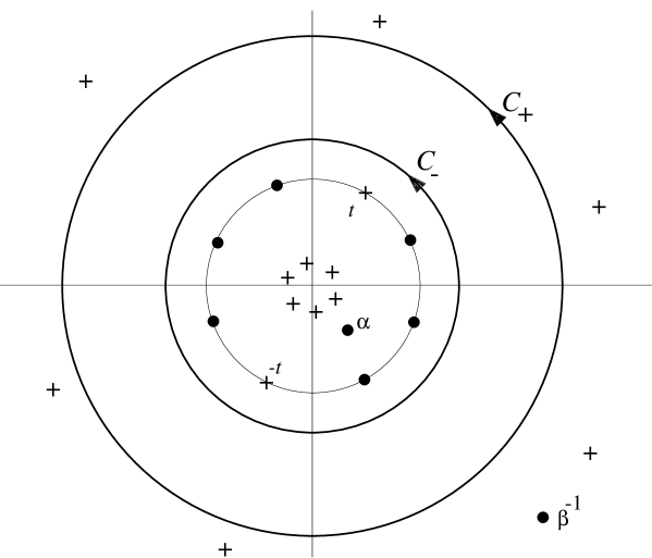
Figure 3: The complex $z$-plane; the curves ${\cal C}_{+}$ and ${\cal C}_{-}$ are indicated, with the unit circle lying inside ${\cal C}_{-}$. The zeros of $\tilde{Q}$ are indicated by $\bullet$ and the zeros of $z^{-1}V(z)$ by $+$. There are no zeros of either function in the annulus between the contours ${\cal C}_{+}$ and ${\cal C}_{-}$.

Draw the contours ${\cal C}_{+}$ and ${\cal C}_{-}$ in the complex $z$-plane, both oriented in the positive direction, with ${\cal C}_{-}$ outside the unit circle, ${\cal C}_{+}$ outside ${\cal C}_{-}$, and such that there are no zeros of $\tilde{Q}(z)$ or $V(z)$ on the boundary of or inside the annulus between ${\cal C}_{-}$ and ${\cal C}_{+}$. Then $\beta^{-1}$ and all the zeros of $B(z)$ lie outside ${\cal C}_{+}$ (see figure 3).

Define $r(z)$ as the quotient of the two terms in the RHS of the functional relation (3.7);

$$r(z)=-\frac{\tilde{Q}(-zx^{-1})(1-z^{2}x)^{N}}{\tilde{Q}(-zx)(1-z^{2}x^{-1})^{N}}$$ (3.11)

($r(z)$ has no zeros or poles on or between the curves ${\cal C}_{+}$ and ${\cal C}_{-}$). Then in the $x\rightarrow 0$ limit, we see that $|r(z)|\sim 1/z^{N}$, so when $|z|>1$, $|r(z)|<1$. Thus $\ln[1+r(z)]$ can be chosen to be single-valued and analytic when $z$ lies in the annulus between ${\cal C}_{-}$ and ${\cal C}_{+}$. We can therefore make a Wiener-Hopf factorisation of $1+r(w)$ by defining the functions $P_{+}(z)$ and $P_{-}(z)$ as

$$\ln P_{\pm}(z)=\pm\frac{1}{2\pi i}\oint_{{\cal C}_{\pm}}\ln\left[1+r(z^{\prime})\right]\frac{dz^{\prime}}{z^{\prime}-z}$$ (3.12)

Then $P_{+}(z)$ is an analytic and non-zero (ANZ) function of $z$ for $z$ inside ${\cal C}_{+}$, and $P_{-}(z)$ is an ANZ function of $z$ for $z$ outside ${\cal C}_{-}$. As $|z|\rightarrow\infty$, we note that $P_{-}(z)\rightarrow 1$. When $z$ is inside the annulus between ${\cal C}_{-}$ and ${\cal C}_{+}$, we have, by Cauchy’s integral formula

$$1+r(z)=P_{+}(z)\>P_{-}(z)=\frac{V(z)\tilde{Q}(z)}{\tilde{Q}(-zx)(1-z^{2}x^{-1})^{N}}.$$ (3.13)

We then define the functions $V_{\pm}(z)$;

$$V_{+}(z) = P_{+}(z)\tilde{Q}(-zx)/(z-\beta^{-1})$$ (3.14)

$$V_{-}(z) = P_{-}(z)(1-z^{2}x^{-1})^{N}\left/\left[\tilde{Q}_{1}(z)(z-\alpha)\right.\right]$$ (3.15)

where $V_{+}(z)$ is an ANZ function of $z$ for $z$ inside ${\cal C}_{+}$, $V_{-}(z)$ an ANZ function of $z$ for $z$ outside ${\cal C}_{-}$. We have split $V(z)$ into two factors, $V_{+}(z)$ and $V_{-}(z)$, with $V(z)=V_{+}(z)V_{-}(z)$ when $z$ is between ${\cal C}_{+}$ and ${\cal C}_{-}$.

Equating (3.10) with the expression $V(z)=V_{+}(z)V_{-}(z)$ we have

$$\frac{V_{+}(z)}{B(z)}=\frac{A(z)}{V_{-}(z)}z(z^{2}-t^{2}).$$ (3.16)

The LHS (RHS) is an ANZ function of $z$ inside ${\cal C}_{+}$ (outside ${\cal C}_{-}$), which is bounded as $|z|\rightarrow\infty$ and so the function must be a constant, $c_{1}$ say. Thus

$$V_{+}(z) = c_{1}B(z)$$ (3.17)

$$V_{-}(z) = c_{1}^{-1}z(z^{2}-t^{2})A(z).$$ (3.18)

When $|z|<1$, we proceed the same way. Draw the curves ${\cal C}_{+}^{\prime}$ and ${\cal C}_{-}^{\prime}$, ${\cal C}^{\prime}_{+}$ inside the unit circle, ${\cal C}_{-}^{\prime}$ inside ${\cal C}_{+}^{\prime}$, and with $\alpha$ and all the zeros of $A(z)$ inside ${\cal C}_{-}^{\prime}$.

In the limit $x\rightarrow 0$, $|1/r(z)|\sim z^{N}$, so $|1/r(z)|<1$. Thus $\ln[1+1/r(z)]$ can be chosen to be single-valued and analytic between and on ${\cal C}_{+}^{\prime}$ and ${\cal C}_{-}^{\prime}$. We can then Wiener-Hopf factorise $1+1/r(z)$ by defining the functions $P_{+}^{\prime}(z)$ and $P_{-}^{\prime}(z)$ as

$$\ln P_{\pm}^{\prime}(z)=\pm\frac{1}{2\pi i}\oint_{{\cal C}^{\prime}_{\pm}}\ln\left[1+\frac{1}{r(z^{\prime})}\right]\frac{dz^{\prime}}{z^{\prime}-z},$$ (3.19)

where $P_{+}^{\prime}(z)$ is ANZ inside ${\cal C}_{+}^{\prime}$, $P_{-}^{\prime}(z)$ is ANZ for $z$ outside ${\cal C}_{-}^{\prime}$. As $|z|\rightarrow\infty$, $P_{-}^{\prime}(z)\rightarrow 1$. When $z$ is in the annulus between ${\cal C}_{+}^{\prime}$ and ${\cal C}_{-}^{\prime}$, Cauchy’s integral formula now implies

$$1+\frac{1}{r(z)}=P_{+}^{\prime}(z)\>P_{-}^{\prime}(z)=-\frac{V(z)\tilde{Q}(z)}{\tilde{Q}(-zx^{-1})(1-z^{2}x)^{N}}.$$ (3.20)

Define $V^{\prime}_{+}(z)$ and $V_{-}^{\prime}(z)$ as follows:

$$V^{\prime}_{+}(z) = P^{\prime}_{+}(z)(1-z^{2}x)^{N}\left/\left[\tilde{Q}_{1}(z)(z-\beta^{-1})\right]\right.$$ (3.21)

$$V_{-}^{\prime}(z) = P^{\prime}_{-}(z)\tilde{Q}(-zx^{-1})/(z-\alpha).$$ (3.22)

We have now factorised $V(z)$ into two factors, $V_{+}^{\prime}(z)$ which is is ANZ for $z$ inside ${\cal C}^{\prime}_{+}$, and $V^{\prime}_{-}(z)$ which is ANZ for $z$ outside ${\cal C}^{\prime}_{-}$. When $z$ is in the annulus between ${\cal C}_{+}^{\prime}$ and ${\cal C}_{-}^{\prime}$, we have the equality $V(z)=V_{+}^{\prime}(z)V_{-}^{\prime}(z)$.

When $z$ is inside this annulus, we equate (3.10) with $V(z)=V^{\prime}_{+}(z)V^{\prime}_{-}(z)$ to get

$$\frac{V_{+}^{\prime}(z)}{B(z)(z^{2}-t^{2})}=\frac{zA(z)}{V_{-}^{\prime}(z)}$$ (3.23)

where now the LHS (RHS) is an ANZ function of $z$ for $z$ inside ${\cal C}^{\prime}_{+}$ (outside ${\cal C}^{\prime}_{-}$). Thus both sides of the equation are constant, $c_{2}$ say, and we have

$$V^{\prime}_{+}(z) = c_{2}(z^{2}-t^{2})B(z)$$ (3.24)

$$V^{\prime}_{-}(z) = c_{2}^{-1}zA(z).$$ (3.25)

From equations (3.17), (3.24) and (3.18), (3.25), we have the following

$$V_{+}^{\prime}(z) = (c_{2}/c_{1})V_{+}(z)(z^{2}-t^{2})$$ (3.26)

$$V_{-}(z) = (c_{1}/c_{2})V_{-}^{\prime}(z)(z^{2}-t^{2}).$$ (3.27)

To evaluate the constant $c_{1}/c_{2}$, consider (3.27) in the limit $z\rightarrow\infty$; we noted earlier that $P_{-}(z)$, $P_{-}^{\prime}(z)\rightarrow 1$ as $z\rightarrow\infty$, so from (3.5), (3.15) and (3.22) we deduce that

$$c_{1}/c_{2}=1.$$ (3.28)

We may use equations (3.26) and (3.27) to derive recurrence relations satisfied by $\tilde{Q}(z)$, which we can solve explicitly in the $N\rightarrow\infty$ limit.

From equations (3.14), (3.21) and (3.26), we deduce the recurrence relation

$$\tilde{Q}(z)\>\tilde{Q}(-zx)=(1-z^{2}x)^{N}\frac{(z-\alpha)(z-\beta^{-1})}{(z^{2}-t^{2})}\frac{P_{+}^{\prime}(z)}{P_{+}(z)}$$ (3.29)

valid when $z$ is inside ${\cal C}_{+}^{\prime}$. In the limit $N\rightarrow\infty$, the $P_{+}$ and $P_{+}^{\prime}$ functions $\rightarrow 1$, so we find that $\tilde{Q}(z)$ is given by

$$\tilde{Q}(z)=\tilde{Q}(0)\prod_{m=1}^{\infty}\left(\frac{1-z^{2}x^{4m-3}}{1-z^{2}x^{4m-1}}\right)^{N}\!\frac{(1-z^{2}t^{-2}x^{4m-2})}{(1-z^{2}t^{-2}x^{4m-4})}\frac{(1-z\alpha^{-1}x^{2m-2})}{(1+z\alpha^{-1}x^{2m-1})}\frac{(1-z\beta x^{2m-2})}{(1+z\beta x^{2m-1})}.$$ (3.30)

This still contains the parameters $t$, $\alpha$ and $\beta$. From (3.29) in the $N\rightarrow\infty$ limit, setting $z=0$ we note that

$$\left[\tilde{Q}(0)\right]^{2}=-t^{-2}\alpha\beta^{-1}.$$ (3.31)

From equations (3.15), (3.22) and (3.27), we get the recurrence relation

$$\tilde{Q}(z)\>\tilde{Q}(-zx^{-1})=(1-z^{2}x^{-1})^{N}\frac{(z-\alpha)(z-\beta^{-1})}{(z^{2}-t^{2})}\frac{P_{-}(z)}{P_{-}^{\prime}(z)}$$ (3.32)

which is valid for $z$ outside ${\cal C}_{-}$. Taking the limit $N\rightarrow\infty$ once more, so that the functions $P_{-}(z)$ and $P_{-}^{\prime}(z)\rightarrow 1$, we get

$$\tilde{Q}(z)=z^{N}\prod_{m=1}^{\infty}\left(\frac{1-z^{-2}x^{4m-3}}{1-z^{-2}x^{4m-1}}\right)^{N}\frac{(1-z^{-2}t^{2}x^{4m-2})}{(1-z^{-2}t^{2}x^{4m-4})}\frac{(1-z^{-1}\alpha x^{2m-2})}{(1+z^{-1}\alpha x^{2m-1})}\frac{(1-z^{-1}\beta^{-1}x^{2m-2})}{(1+z^{-1}\beta^{-1}x^{2m-1})}.$$ (3.33)

To derive an expression for $V(z)$ valid between ${\cal C}_{+}$ and ${\cal C}_{-}^{\prime}$, using equation (3.27), we have

$$V(z) = V_{+}(z)V_{-}^{\prime}(z)(z^{2}-t^{2})$$ (3.34)

$$= \tilde{Q}(-zx)\tilde{Q}(-zx^{-1})(z^{2}-t^{2})\left/\left[(z-\alpha)(z-\beta^{-1})\right]\right..$$

We use (3.30) for $\tilde{Q}(-zx)$ and (3.33) for $\tilde{Q}(-zx^{-1})$, and substitute into equation (3.34). This produces a lengthy expression for $V(z)$ involving the parameters $\alpha,\beta$ and $t$, which simplifies when one considers the oddness of $V(z)$. The poles of $V(z)$ must occur in pairs, and this is only possible if $\alpha$ and $\beta$ are related by

$$\alpha\beta=-x.$$ (3.35)

Substituting this in, the infinite products involving $\alpha$ and $\beta$ cancel, and we get, from (3.6) and (3.34)

$$\Lambda(v)=G(z/t)\>(\rho/2x)^{N}\prod_{m=1}^{\infty}\left(\frac{1-z^{2}x^{4m-1}}{1-z^{2}x^{4m+1}}\cdot\frac{1-z^{-2}x^{4m-1}}{1-z^{-2}x^{4m+1}}\right)^{N}$$ (3.36)

where

$$G(z)=\pm ix^{1/2}(z-z^{-1})\prod_{m=1}^{\infty}\left(\frac{1-z^{2}x^{4m}}{1-z^{2}x^{4m-2}}\cdot\frac{1-z^{-2}x^{4m}}{1-z^{-2}x^{4m-2}}\right).$$ (3.37)

This expression for the eigenvalue is still dependent on the parameter $t$, different values of $t$ corresponding to different eigenvalues of the transfer matrix. All we know about $t$ so far is that it is bounded as $x\rightarrow 0$, and that it lies on the unit circle in the $x\rightarrow 0$ limit. We shall now show that it in fact remains exactly on the unit circle as $x$ increases.

We substitute into the functional relation (3.7), using equations (3.30) and (3.33) to get an expression for the product $\tilde{Q}(z)V(z)$ which is valid when $z$ is in the annulus between ${\cal C}_{+}$ and ${\cal C}_{-}^{\prime}$. Substituting into (3.7), the function on the right hand side is equal to zero when $z$ is one of the $N-2$ zeros of $\tilde{Q}_{1}(z)$, or when $z=\pm t$. For the latter case, substituting $z=t$ and $-t$, and dividing the resulting equations, we arrive at the following relation between $\alpha,x,$ and $t$

$$\alpha^{2}=-t^{2}x$$ (3.38)

which means that $t$ must satisfy

$$\left[\phi(t)\right]^{N}=\pm 1$$ (3.39)

where $\phi(t)$ is given by

$$\phi(t)=t\prod_{m=1}^{\infty}\left(\frac{1-t^{2}x^{4m-1}}{1-t^{2}x^{4m-3}}\cdot\frac{1-t^{-2}x^{4m-3}}{1-t^{-2}x^{4m-1}}\right).$$ (3.40)

This implies that $t$ lies on the unit circle for all $x$, there being $2N$ possible choices for $t$. The partition function depends on $t$ only via $t^{2}$, so there are only $N$ distinct eigenvalues. The right hand side of (3.7) also vanishes when $z$ is a zero of $\tilde{Q}_{1}(z)$ so in the same way we show that the zeros of $\tilde{Q}_{1}(z)$ lie exactly on the unit circle for all $x$. As the zeros lie exactly on the unit circle, we may shift the curves ${\cal C}_{-}$ and ${\cal C}_{+}^{\prime}$ so that they just surround the unit circle. Hence our expressions for $\tilde{Q}(z)$ are valid all the way up to the unit circle; (3.30) is valid for $|z|<1$, and (3.33) is valid for $|z|>1$.

We now evaluate the partition function, as defined in (3.1), in the large-lattice limit. When $v$ is real, the eigenvalues (3.36) are complex, so as $N\rightarrow\infty$, the partition function, a sum over the $N$ eigenvalues defined by (3.39), becomes an integral over all the allowed values of $t$,

$$Z=\oint\rho(t)\left[\Lambda(v)\right]^{M}dt$$ (3.41)

where the integral is taken around the unit circle, and $\rho(t)$ is some distribution function, independent of $N$ and $M$. Substituting (3.34) into (3.41) then gives an expression for $Z$. (The number of rows $M$ is even to ensure periodic boundary conditions vertically, and so the $\pm$ sign in (3.37) is irrelevant.)

The eigenvalue (3.36) contains two distinct types of factors; those that are powers of $N$, and those that are not. The terms that increase exponentially with $N$ contribute to the bulk part of the partition function, the free energy per site in the thermodynamic limit. This factor is also independent of $t$, and can be taken out of the integral (3.41). The integral is then independent of $N$, so we have, from (3.2)

$$e^{-f/k_{B}T}=(\rho/2x)\prod_{m=1}^{\infty}\left(\frac{1-z^{2}x^{4m-1}}{1-z^{2}x^{4m+1}}\cdot\frac{1-z^{-2}x^{4m-1}}{1-z^{-2}x^{4m+1}}\right)$$ (3.42)

for the free energy per site in the thermodynamic limit. This result agrees with the result for periodic boundary conditions (equations (8.9.9) and (8.9.10) of Ref. [1]).

From equation (3.2), the other factors in (3.34) make up the interfacial tension, given by

$$e^{-Ms/k_{B}T}=\oint\rho(t)\left[G(z/t)\right]^{M}dt.$$ (3.43)

For $M$ sufficiently large, we may evaluate this integral using saddle-point integration. The integral is given by the value of the integrand at its saddle point, together with some multiplicative factors that we can disregard as $M\rightarrow\infty$. The function $G$ satisfies the relation

$$G(z)=G(-1/z)$$ (3.44)

which implies that the function has a saddle point when $z=\pm i$. Hence the integrand in (3.43) is maximised when

$$t=t_{\rm saddle}=\pm iz.$$ (3.45)

As $z$ is arbitrary, this point may lie off the unit circle; it will however lie inside the annulus between ${\cal C}_{+}$ and ${\cal C}^{\prime}_{-}$ because of the restriction (3.4), and so we will be able to deform the contour to pass through this saddle point. Hence we arrive at the final result

$$\mbox{\rm e}^{-s/k_{B}T}=2x^{1/2}\prod_{m=1}^{\infty}\left(\frac{1+x^{4m}}{1+x^{4m-2}}\right)^{2}.$$ (3.46)

Figure 1: Standard vertex configurations and corresponding weights.

Figure 2: A typical lowest-energy state of the system with $N$ even and anti-periodic boundary conditions. The dotted line indicates the interface dividing the lattice into two domains, each of which is an anti-ferroelectrically ordered ground state.

References

[1]
Baxter R J 1982 Exactly Solved Models in Statistical Mechanics
(London: Academic)
[2]
Lieb E H and Wu F Y 1972 in Phase Transitions and Critical Phenomena
vol 1, ed C Domb and M S Green (London: Academic) p 321
[3]
Sklyanin E K, L Takhtajan and L Faddeev 1979
Theor. Maths. Phys.40 194
[4]
Kulish P P and Sklyanin E K 1982 in Lecture Notes in Physics vol 151,
ed J Hietarinta and C Montonen (Berlin: Springer-Verlag) p 61
[5]
Reshetikhin N Yu 1983 Sov. Phys. JETP57 691
[6]
de Vega H J 1984 Nucl. Phys. B240 495
[7]
Baxter R J 1972 Ann. Phys. (N.Y.)70 193
[8]
Baxter R J 1973 J. Stat. Phys.8 25
[9]
Alcaraz F C, Baake M, Grimm U and Rittenberg V 1988
J. Phys. A21 L117
[10]
Yung C M and Batchelor M T 1995 Exact solution for the spin-
quantum chain with non-diagonal twists, ANU preprint
[11]
Johnson J D, Krinsky S and McCoy B M 1973 Phys. Rev. A8 2526
[12]
Onsager L 1944 Phys. Rev.65 117
[13]
Noble B 1958 Methods Based on the Wiener-Hopf Technique (London:
Pergamon)