IMSc-94/52

Infrared Behaviour of Systems With Goldstone Bosons
Ramesh Anishetty, Rahul Basu, N.D. Hari Dass and H.S.Sharatchandra

The Institute of Mathematical Sciences, Madras-600 113, INDIA

We develop various complementary concepts and techniques for handling quantum fluctuations of Goldstone bosons.We emphasise that one of the consequences of the masslessness of Goldstone bosons is that the longitudinal fluctuations also have a diverging susceptibility characterised by an anomalous dimension $(d-2)$ in space-time dimensions $2<d<4$.In $d=4$ these fluctuations diverge logarithmically in the infrared region.We show the generality of this phenomenon on the basis of i). Renormalization group flows, ii). Ward identities, and iii). Schwinger-Dyson equations.We also obtain an explicit form for the generating functional of one-particle irreducible vertices of the O(N) (non)–linear $\sigma$–models in the leading $1/N$ approximation.We show that this incorporates all infrared behaviour correctly both in linear and non-linear $\sigma$– models. These techniques provide an alternative to chiral perturbation theory.Some consequences are discussed briefly.

1 Introduction

The concept of spontaneous breaking of a continuous global symmetry with the attendant Goldstone phenomenon of massless scalar excitations has deeply influenced many developments in field theory and statistical physics. The existence of massless modes can already be demonstrated in Landau - Ginzberg mean field analysis (or tree level, in the field theory jargon). However, it is not sufficient to stop at this level. Precisely because they are massless, the quantum/statistical fluctuations of the Goldstone bosons may significantly alter the conclusions drawn from mean field theory.Proofs of the Goldstone theorem [1] in quantum field theory have traditionally been used only to establish the existence of massless poles coupling to the currents of broken symmetry. They have not usually focussed on the correlation functions. Most of the applications in quantum field theory have been based on the understanding at tree level. Notable exceptions are the soft pion theorems [2] combining PCAC with current algebra.These are mostly applied to extract the leading infrared behaviour. A general analysis of these issues based essentially only on symmetry arguments was given some time ago by Weinberg [4]. In that article he also proposed methods to go beyond the leading order results. He also applied renormalization group methods to understand some universal features of these results. Quite recently, some of Weinberg’s ideas have been extensively used in the context of the so called “chiral perturbation theory”[5].

In contrast, in statistical physics, powerful techniques have been developed for handling the fluctuations in this context. These are of importance for quantum field theory also.Some examples are: i)the finite temperature chiral symmetry restoring transition in QCD, where Goldstone phenomenon in three Eucilidean dimensions is of relevance [3]; ii)QCD at temperatures below the chiral transition temperature as well as zero temperature QCD, where Goldstone phenomenon in 4 euclidean dimensions is of relevance,and iii)the problems that are handled by chiral perturbation theory at present, i.e. effects of pion loops on various processes [5].

In this paper we point out various complimentary concepts and techniques for handling the effects due to quantum fluctuations of Goldstone bosons. We develop techniques for computing correlation functions away from the infrared regime.We show that there are certain universal features, valid even in four space-time dimensions.Our approach provides an alternate procedure for chiral perturbation theory which is closer in its spirit to what has been proposed by Weinberg on the basis of RG equations. This aspect is elaborated upon in section 7.

2 Infrared dynamics of pions and sigma

Often the paradigm in quantum field theory is what is seen from a tree level analysis of the O(N) linear and non-linear $\sigma$-models. The linear $\sigma$-model is given by the action [8],

$$S=\int d^{d}x(\frac{1}{2}(\partial_{\mu}\vec{\Phi}(x))^{2}-\frac{U}{4}(\vec{\Phi}^{2}(x)-C^{2})^{2})$$ (1)

$\vec{\Phi}=\{\Phi_{i},i=1,2,....N\}$ transforms as the fundamental representation of O(N). If $C^{2}>0$, the minimum of the classical potential is at $\vec{\Phi}^{2}=C^{2}$. Therefore the VEV $<\vec{\Phi}>$ is no longer zero in a tree level analysis.Choosing the vacuum $<\Phi_{N}>=C,<\Phi_{i}>=0,i=1,2,...(N-1)$, among the equivalent vacua, we get,

$$S = \int d^{d}x(\frac{1}{2}(\partial_{\mu}\vec{\pi}(x))^{2}+\frac{1}{2}(\partial_{\mu}\sigma(x))^{2}-UC^{2}\sigma^{2}(x)$$ (2)

$$-UC\sigma(x)(\sigma^{2}(x)+\vec{\pi}^{2}(x))-\frac{U}{4}(\sigma^{2}(x)+\vec{\pi}^{2}(x))^{2}$$

where $\sigma=\Phi_{N}-<\Phi_{N}>,\vec{\pi}=\{\Phi_{i},i=1,2,...(N-1)\}$. Therefore at tree level, we have $(N-1)$ massless pions and a massive $\sigma$ with a mass $\sqrt{2UC^{2}}$.

Precisely because the Goldstone bosons are massless, loop corrections may drastically alter the above picture. Now it is well known that infrared divergences due to massless fluctuations drastically alter the conclusions of a semi-classical analysis, especially if the spacetime dimension d is less than four [8].Already, way back in 1940, Holstein and Primakoff [9] argued that not only the transverse mode (i.e. $\pi$) but also the longitudinal mode ($\sigma$) is soft in a quantum ferromagnet in three dimensions. Their arguments can be understood,as follows, in terms of the non-linear $\sigma$ -model.

The non-linear $\sigma$- model is relevant to the infrared dynamics of Goldstone bosons [8] .A simple heuristic argument is that if $\sigma$ is massive, then for the study of the infrared dynamics of the pions, we may use an effective Lagrangian obtained by integrating over the heavy $\sigma$ degree of freedom. Also for leading infrared behaviour we may retain only the lowest (two) derivative terms in the effective action.The result is simply the Heisenberg model,

$$S_{NL}=\frac{1}{2t}\int d^{d}x(\partial_{\mu}\vec{\phi}(x))^{2}$$ (3)

with the constraint, $\vec{\phi}^{2}(x)=1$. Statistical physics in d space dimensions is simply the Euclidean quantum field theory in $d$ space-time dimensions. In statistical physics $t$ is proportional to the temperature, whereas in quantum field theory it is related to the pion decay constant, $t=2f_{\pi}^{-2}$(in what follows, we set $f_{\pi}=1$). If the spins are ordered in the direction of $\phi_{N}$, then eliminating this field using the constraint, the action can be written entirely in terms of $\vec{\pi}=\{\phi_{i},i=1,2,...(N-1)\}$. They describe the spin waves or the transverse fluctuations.At the tree level for the $\pi$ propagator we get,

$$\Delta_{\pi}(k)=k^{-2}$$ (4)

We may also consider the correlations for longitudinal fluctuations i.e. of the field $\sigma=\phi_{N}\sim:\sqrt{1-\vec{\pi}^{2}}:-1$(: refers to any ordering prescription that makes products of fields at the same point meaningful). This means, $\sigma\sim:\vec{\pi}^{2}:+\frac{1}{4}:\vec{\pi}^{4}:+.....$. We may expect the leading infrared behaviour to come from the first term. This would mean that so far as the leading infrared behaviour is concerned, [10], [11] $\sigma\sim:\bf\pi^{2}:$. If we ignore self-interactions of $\bf\pi$, and use the above propagator for $\bf\pi$ we get,for the $\sigma$ propagator,

$$\Delta_{\sigma}(x)=\Delta_{\pi}^{2}(x)=\mid{x}\mid^{4-2d}$$ (5)

This gives, atleast for $d<4$,in momentum space,

$$\Delta_{\sigma}(k)=\mid{k}\mid^{d-4}$$ (6)

Ignoring the self interactions of $\pi$’s will later be seen to be justified because these are soft in the infrared region– a consequence of the soft pion theorems.The result is that in $d=3$ the $\sigma$–propagator is $\mid{k}\mid^{-1}$, to be contrasted with the $\pi$-propagator.This means that $\sigma$ also has long range correlations. This appears to negate the naive deduction of the non-linear $\sigma$ model obtained by integrating over the heavy $\sigma$ field in the linear $\sigma$ model [12].

One could dismiss these results as artifacts of a 1-loop calculation. In fact the infrared divergences grow with the loop order. Therefore it is imperative to tackle this issue in a framework that transcends loop expansion.There is an exactly solvable model, the Berlin-Kac model [13] which goes beyond loop-expansion and again gives precisely the same diverging longitudinal susceptibility and also a massless $\sigma$ in $d<4$. Again it is not clear whether this is an artifact of the model.

In order to get a handle on the infrared dynamics of the $\sigma$ field, Pokrovsky and Patashinky [14] proposed a ”Conserved Modulus Principle” (CMP).This principle holds that the fluctuations are such as to maintain the modulus of the N- component order parameter. In mathematical terms CMP states that

$$2<\phi>\delta\phi_{L}+\delta\phi_{T}^{2}=0$$ (7)

Now the expectation value of $\delta\phi_{T}^{2}$ is given by the Ornstein- Zernike form:

$$\delta\phi_{T}^{2}=\int{d^{d}q\over{q^{2}+H/<\phi>}}$$ (8)

It is convenient to use susceptibility to describe the infrared behaviour.The longitudinal and the transverse susceptibility in presence of an external magnetic field $\vec{H}=(0,0,...,0,H)$ are given by ,

$$\chi_{L}=lim_{k\rightarrow 0}\Delta_{\sigma}(k^{2}),\ \ \chi_{T}=lim_{k\rightarrow 0}\Delta_{\pi}(k^{2})$$ (9)

Using Eqns. 7 and 8, we get, for $d<4$,

$$\chi_{L}={\partial(\delta\phi_{L})\over\partial H}\sim(H)^{d/2-2}~{}~{}~{}~{}~{}~{}\chi_{T}\sim H^{-1}$$ (10)

Thus the longitudinal suceptibility also diverges. Patashinsky and Pokrovski have offered a proof for CMP in [15]. They express the change in the thermodynamic potential U computed to quartic order in the fluctuations as

$$\delta U=1/2[{(\delta\phi_{T})^{2}\over\chi_{T}}+{(\delta\vec{\phi}^{2})^{2}\over 4\chi_{L}\bar{\phi}^{2}}]$$ (11)

and interpret this as implying CMP. Though to quartic order the correct form of this variation, which differs from the one given above (and which can be verified using the Ward identities discussed later), is

$$\delta U={1\over 2\chi_{T}}[(\delta\phi_{T})^{2}+(\delta\phi_{L})^{2}-{(\delta\vec{\phi}^{2})^{2}\over 4\bar{\phi}^{2}}]+{1\over 2\chi_{L}}[{(\delta\vec{\phi}^{2})^{2}\over 4\bar{\phi}^{2}}]$$ (12)

the fact that CMP is equivalent to the correct statement that the extreme IR behaviour is governed by the non-linear $\sigma$-model indicates the possibility of a better proof of CMP.

The new era for understanding the role of fluctuations of Goldstone bosons started with the renormalization group techniques. Brezin, Wallace and Wilson [16] computed the equation of state for O(N) $\sigma$–model using the $\epsilon$–expansion.They found important differences from the corresponding calculation for the N=1 case (i.e. the Ising model).This could be traced to the infrared singularities due to the Goldstone bosons that are present everywhere in the coexistence region for $N>1$. In particular it meant that the conclusions of the tree level analysis could not be right (atleast for $d<4$).

At the critical point ($T=T_{c},H=0$), $\sigma$ and $\pi$ are on the same footing. Both their susceptibilities diverge with vanishing magnetic field as,

$$\chi_{T}=\chi_{L}\sim H^{{1\over\delta}-1}$$ (13)

governed by the critical exponent $\delta$. The question of interest is the behaviour for $T<T_{c}$ as $H\rightarrow 0$.The assumption that the singularities due to Goldstone bosons exponentiate in the $\epsilon$–expansion suggested that,

$$\chi_{T}\sim H^{-1},\quad\chi_{L}\sim H^{-\epsilon/2}$$ (14)

Holstein -Primakoff [9], Berlin-Kac [13], and Patashinski-Pokrovski [14] models have all made the same prediction. Such a result has also been proved rigorously for O(2) case using correlation inequalities in Ref. [17].

A deeper understanding can be obtained by considering the renormalization group flows shown in the figure below:

Figure 1: The fixed point structure of the O(N) sigma model; the arrows indicate infrared flows

At the critical point, $T=T_{c},H=0$, the infrared dynamics is governed by the O(N) non-Gaussian fixed point ${\cal NG}_{N}$ when $2<d<4$.Everywhere on the critical surface the renormalization group (RG) trajectories flow from the the O(N) Gaussian fixed point ${\cal G}_{N}$ (which is infrared unstable) to the O(N) non-Gaussian fixed point ${\cal NG}_{N}$. For $T>T_{c}$ we have the symmetric phase with massive (and degenerate) $\sigma$ and $\vec{\pi}$.The infrared behaviour is governed by the trivial fixed point $\cal T$ which corresponds to zero correlation length.$T<T_{c}$ presents a new feature compared to N=1 case (i.e.the Ising model). The theory has long range correlations for all $T<T_{c},H=0$ as a consequence of the Goldstone phenomenon.Hence the infrared behaviour must be determined by a fixed point of infinite correlation length.What is this fixed point?

$T-T_{c}$, the deviation from the critical temperature in statistical mechanics, is to be identified with the square of the renormalized mass [8] in the linear $\sigma$-model. In particular they are parameters with positive mass dimensionality. Under RG flow they necessarily scale.Thus, once $T-T_{c}<0$, the flow is towards $T=0$.This means that we are interested in the zero temperature fixed point. An indication as to the nature of this fixed point came from a study of $2+\epsilon$–expansion of O(N) non–linear $\sigma$–model by Brezin and Zinn-Justin [18].

The O(N) non-linear $\sigma$- model in d=2 is renormalizable. Even though the renormalized perturbation is in terms of the spin wave modes, Mermin-Wagner theorem [8] requires that the system is never in a phase with spontaneously broken O(N) symmetry. A hint of this is contained in the renormalized perturbation theory: the theory is asymptotically free.The coupling constant grows with the distance so that the long distance structure of the theory could be drastically different from the perturbation theory spectrum.Indeed the spectrum is believed be that of massive and degenerate $\sigma$ and $\pi$’s in the fundamental representation of O(N).

A consequence of the asymptotic freedom in $d=2$ is that in $d=2+\epsilon$, the $\beta$-function $\beta(t)$ has a non-trivial zero (say at $t=t_{c}$) in addition to the trivial zero, $t=0$, corresponding to the theory of (N-1) free scalars.At $t=t_{c}$ the theory is scale invariant and corresponds to the critical theory with N massless scalars and with anomalous dimensions ( denoted by ${\cal NG}^{*}_{N}$ ).It should be noted in Fig. 1 that the fixed point ${\cal NG}_{N}$ of the linear $O(N)$-model is identified with the fixed point ${\cal NG}^{*}_{N}$ of the non-linear model. This follows essentially from a remark made in [8] that at ${\cal NG}_{N}$ the correlation functions of the linear model are identical to those of the non-linear model where in the latter one includes correlation functions of composite operators also. The coincidence of these two fixed points can also be established in the $1/N$-expansion scheme [19]. For $t>t_{c}$, the coupling constant grows with the distance, and as in $d=2$, the theory is in the unbroken phase. $t<t_{c}$ is of interest to us.In this case the infrared flow is towards $t=0$. The infrared behaviour is of O(N-1) Gaussian theory (This fixed point is denoted by ${\cal G}_{N-1}$ in Fig.1.) and the ultraviolet behaviour is of the critical theory with anomalous dimensions.

The fact that the infrared behaviour for $t<t_{c}$ is governed by the O(N-1) Gaussian fixed point gives exhaustive information on the effects of quantum fluctuations of the Goldstone bosons.It means that the pions decouple from each other at low momenta, and their propagators behave as the free propagators for small momenta.It also allows us to obtain the non-leading IR-behaviour as well as the effects of an external magnetic field.In particular we now understand why various heuristic considerations all gave the correct answer: it was the fortuitious behaviour of a free massless theory.Anything more complicated would have been much more difficult to handle.

Upto what dimension d is the analysis of $d=2+\epsilon$ calculation correct?In particular is it applicable to d=4?The case d=4 is somewhat different because of the absence of the non-Gaussian fixed point ${\cal NG}_{N}$.At the critical temperature the infrared behaviour is believed to be given by free massless theory of N scalars as the beta function is positive for small couplings; there is no evidence for a non-Gaussian fixed point.This appears to exclude the validity of the $2+\epsilon$ analysis to this case.We need an alternate technique to handle this situation.This is provided ,for example,by the $1/N$ expansion.

The $1/N$ expansion provides results which agree with the above analysis for all d.(The Berlin-Kac model [13] is a variant of this technique.) It yields the non-Gaussian fixed point for $2<d<4$ and shows its absence for $d=4$.In either case it shows that the leading infrared behaviour anywhere in the broken phase is given by N-1 free pions.The only handicap of this technique is that it does not provide non-anomalous dimension for the non-Gaussian fixed point ${\cal NG}_{N}$ in the leading N approximation.However even this is overcome once one takes higher order (in $1/N$) corrections. There are also indications that the technique gives qualitatively correct and quantitatively reasonable results for all $N>2$.

The fact that even in d=4 the pion dynamics is governed by the O(N-1) Gaussian fixed point ${\cal G}_{N-1}$ in the infrared has important implications.In particular the propagator of $\sigma$ (to be interpreted as the O(N) partner of the pions) has an universal logarithmic singularity in the infrared region,

$$\Delta_{\sigma}(k)\sim ln(\frac{\mu}{k^{2}})$$ (15)

where $\mu$ is the renormalisation scale. This follows from the same arguments as for $d<4$, in particular because $\sigma\sim:\bf\pi^{2}:$ in the infrared.This feature is present whether $\sigma$-propagator has a pole at some $k^{2}\neq 0$ or not. The precise location of the pole is a non-universal feature depending on the microscopic dynamics. It could have interesting implications for nuclear forces at low energies in the ’sigma’-channel (i.e., spin J=0,isospin I=0) as will be discussed elsewhere.

In Sec. 3 and 4 we develop a new formalism for $N\rightarrow\infty$ which will allow for explicit calculation of all correlation functions even away from the infrared regime.We will explicitly demonstrate all the properties mentioned above.Our formalism gives the same results in the leading infrared limit whether one starts with the linear or the non-linear $\sigma$- model.

That the pions behave like free massless bosons in the infrared limit, in any $d>2$, is such a general phenomenon that there should be an easier way of understanding it. A careful analysis of the proof of the Goldstone theorem along with current algebra and PCAC provide one such non-perturbative argument.Another is the treatment based on Ward identities given in sec 5.Low energy theorems based on PCAC and current algebra do imply that pions decouple from each other and with other matter at low momenta, but they do not directly imply that the pion has a canonical dimension in the infrared.Current algebra requires that the current coupling to the pion has canonical dimension $d-1$. However, the canonical dimension (for the $k\rightarrow 0$ behaviour of the pion) is $(d-2)/2$. This only means that the PCAC relating the two needs a dimensionful parameter, but does not directly relate the two dimensions.

Consider the time ordered correlation function of a current in a broken direction and the corresponding $\pi$ field:

$$\Delta^{ii}_{\mu}(x)=<0\mid T(j_{\mu}^{i}(x),\pi^{i}(\bf 0))\mid 0>$$ (16)

We get,

$$\int d^{d}x\partial^{\mu}\Delta^{ii}_{\mu}(x)=<0\mid[Q^{i},\pi^{i}(0)]\mid 0>\not=0$$ (17)

since $[Q^{i},\pi^{i}(0)]=\sigma(0)$ has a non-zero expectation value. This means for the Fourier transform of this correlation function,

$$lim_{q\rightarrow 0}q^{\mu}\Delta^{ii}_{\mu}(q)\neq 0$$ (18)

This requires that in the spectral representation of the correlation function there is necessarily a $\delta(m^{2})$ contribution implying a simple pole at zero mass.Any other singularity, such as a branch point will not satisfy the above equation.

The fact that the $\sigma$ channel also has an infrared singularity is equally general and should be understandable in a general way. In Sec. 5 and 6 we provide two proofs which rely essentially on symmetry arguments. The first uses Ward identities, and the second, the Schwinger- Dyson equations.

3 $\Gamma$ in $N\rightarrow\infty$ limit

It was argued in Sec. 2 that the leading term in $1/N$ expansion retains all important effects of the Goldstone boson fluctuations. Analytic calculations are possible in this limit and therefore we can analyse such effects in detail.There is an extensive literature on this technique [8].In this section we provide a new arsenal to this technique.We define a generalized generating functional of one-particle irreducible (1PI) vertices and obtain an explicit expression for it in the large N limit. This is made possible by involving an auxiliary field. Our method provides the easiest way of extracting all correlation functions without doing a separate calculation for each [20]. We present results for both linear and non-linear $\sigma$-models.

$W[\vec{H}]$, the generating functional of connected Green’s functions, is given by,

$$e^{iW[\vec{H}]}=\int{\cal D}{\vec{\Phi}}e^{i(S[{\vec{\Phi}}]+{\vec{H}}.{\vec{\Phi}})}$$ (19)

where,

$$\vec{H}.\vec{\Phi}=\int d^{d}x\vec{H}(x).\vec{\Phi}(x)$$ (20)

Connected Green’s functions of $\Phi_{i}$ are obtained from various functional derivatives of $W[\vec{H}]$. $\Gamma[\vec{\Phi}]$, the generating functional of 1PI vertices, is obtained from $W[\vec{H}]$ by a Legendre transformation.

$$\Gamma[\vec{\Phi}]=W[\vec{H}]-\vec{H}.\vec{\Phi}$$ (21)

where,

$$\Phi_{i}(x)=\frac{\delta W[\vec{H}]}{\delta H_{i}(x)}$$ (22)

The vacuum expectation value (VEV) of $\Phi_{i}$ is obtained as the value at which $\Gamma$ is minimized.The second functional derivative about this minimum gives the inverse propagator. Further, various functional derivatives of $\Gamma$ about this minimum give the 1PI vertices. The connected Green’s functions can be extracted by building only tree diagrams using these propagators and vertices.

In the linear $\sigma$-model, introduce an auxiliary field $\lambda$ to make the exponent bilinear in $\vec{\Phi}$:

$$e^{iW[\vec{H}]}=\int{\cal D}\lambda{\cal D}{\vec{\Phi}}e^{i\int d^{d}x(\frac{1}{2}(\partial_{\mu}{\vec{\Phi}}(x))^{2}-\frac{1}{2}\lambda(x)({\vec{\Phi}}^{2}(x)-C^{2})+\frac{1}{4U}\lambda^{2}(x)+{\vec{H}}(x)\cdot{\vec{\Phi}}(x)}$$ (23)

Now an integration over each $\Phi_{i},i=1,2....,N$, gives a $(Det)^{-1/2}$ factor. Therefore,

$$e^{iW[\vec{H}]}=\int{\cal D}\lambda e^{i\int d^{d}x(\frac{1}{4U}\lambda^{2}(x)+\frac{C^{2}}{2}\lambda(x))-\frac{N}{2}Trln\nabla-i\frac{1}{2}H.\nabla^{-1}.H}$$ (24)

where,

$$\nabla(x,y)=(-\partial^{2}-\lambda(x))\delta(x-y)$$ (25)

On defining,

$$NU=u,C^{2}=Nc^{2},H_{i}=\sqrt{N}h_{i},W[{\vec{H}}]=Nw[{\vec{h}}]$$ (26)

We get,

$$e^{iNw[{\vec{h}}]}=\int{\cal D}\lambda e^{iN[(\int d^{d}x(\frac{1}{4u}\lambda^{2}+\frac{1}{2}c^{2}\lambda))+\frac{i}{2}Trln\nabla-\frac{1}{2}h.\nabla^{-1}.h]}$$ (27)

We are interested in the limit $N\rightarrow\infty$, $U\rightarrow 0$ holding $NU=u$ fixed. With the variables redefined as in Eqn. 26, it is clear that this limit is dominated by the saddle point. The fluctuations about the saddle point give contributions which are non-leading in N. Thus the leading contribution is,

$$w_{\infty}[{\vec{h}}]=\int d^{d}x(\frac{1}{4u}\lambda^{2}(x)+\frac{1}{2}c^{2}\lambda(x))\\ +\frac{i}{2}Trln\nabla-\frac{1}{2}h.\nabla^{-1}.h$$ (28)

where $\lambda(x)$, the saddle point, is a functional of $\vec{h}(x)$ as given by,

$$\frac{1}{u}\lambda(x)+c^{2}-i\nabla^{-1}(x,x)-(h.\nabla^{-1})(x).(\nabla^{-1}.h)(x)=0$$ (29)

We may obtain $\Gamma[\vec{\Phi}]$ from $w_{\infty}[{\vec{h}}]$ by a Legendre transform as described earlier. But this form is not easily amenable to further analysis. Instead we note that the saddle point equation may be rewritten as

$$\frac{1}{u}\lambda(x)+c^{2}-i\nabla^{-1}(x,x)=\vec{\phi}^{2}(x)$$ (30)

where,

$$\nabla\phi_{i}(x)=-h_{i}(x)$$ (31)

Notice that these equations can be obtained from the following functional of $\vec{\phi}$ and $\lambda$ :

$$\Gamma_{\infty}[\vec{\phi},\lambda] = \int d^{d}x(\frac{1}{4u}\lambda^{2}(x)+\frac{1}{2}c^{2}\lambda(x)+\frac{1}{2}(\partial_{\mu}\vec{\phi})^{2}(x)$$ (32)

$$-\frac{1}{2}\lambda(x)\vec{\phi}^{2}(x))+\frac{i}{2}Trln\nabla$$

by taking functional derivatives:

$$-h_{i}(x)=\frac{\delta\Gamma_{\infty}[\vec{\phi},\lambda]}{\delta\phi_{i}(x)},\quad-\kappa(x)=\frac{\delta\Gamma_{\infty}[\vec{\phi},\lambda]}{\delta\lambda(x)}$$ (33)

Here we have temporarily added a ’source’ $\kappa$ for $\lambda$.When restricted to correlation functions with only $\phi_{i}$ on external legs, $\kappa$ can be set to zero, yielding eqn 30. These equations imply that $w_{\infty}[\vec{h},\kappa]$ and $\Gamma_{\infty}[\vec{\phi},\lambda]$ are related by a functional Legendre transformation in both arguments. This means that the connected Green’s functions of $\vec{\phi}$ and in fact also of $\vec{\phi}^{2}$ (i.e. functional derivatives of $w_{\infty}[\vec{h},\kappa]$ wrt both $\vec{h}$ and $\kappa$) can be obtained from tree diagrams built from the ’action’ $\Gamma_{\infty}[\vec{\phi},\lambda]$.This connection is simply an algebraic consequence of the Legendre transformation. We have thus the option of constructing Green’s functions involving the composite operator $:\phi^{2}:$ also by having $\lambda$ as external legs.

By introducing an auxiliary field $\lambda$ we have obtained an explicit form of the generating functional of 1PI vertices which is far more amenable to analysis than if we had obtained a $\Gamma(\vec{\phi})$ by substituting the saddle point solution for $\lambda$ .Moreover we find that the properties of the phase with spontaneously broken symmetry can be understood in a simple way in terms of this auxiliary field. Ofcourse, now $\lambda$ also appears in propagators and vertices. The usual generating function $\Gamma[\phi]$ can however be recovered by using $\kappa=0$ from Eq.33 to replace $\lambda$ as a functional of $\phi$ in $\Gamma_{\infty}[\vec{\phi},\lambda]$.

There is hardly any change in our calculations (and results) when passing over to the non-linear $\sigma$-model. Now we have,

$$e^{iW_{NL}[\vec{H}]}=\int{\cal D}\vec{\Phi}\Pi_{x}\delta^{d}(\vec{\Phi}^{2}(x)-C^{2})e^{i\int d^{d}x(\frac{1}{2}(\partial_{\mu}\vec{\Phi}(x)^{2}+\vec{H}(x)\cdot\vec{\Phi}(x)})$$ (34)

Using the Fourier representation for the functional $\delta$ function,

$$e^{iW_{NL}[{\vec{H}}]}=\int{\cal D}\lambda{\cal D}\vec{\Phi}e^{i\int d^{d}x(\frac{1}{2}(\partial_{\mu}\vec{\Phi}(x)^{2})-\frac{1}{2}\lambda(\vec{\Phi}^{2}(x)-C^{2})+\vec{H}(x)\cdot\vec{\Phi}(x))}$$ (35)

In this form the only difference with the linear $\sigma$-model is that a quadratic term in $\lambda$ is missing in the exponent.Equivalently, the non-linear $\sigma$-model is simply the special case $U\rightarrow\infty$ of the linear $\sigma$-model. Thus all results for the non-linear $\sigma$-model can be extracted by taking this limit in our formulae.We find that it is straightforward to take this limit and the results are not very different.

We have been cavalier in our manipulations with the functional integrals.For instance, the $Trln$ term has to be carefully defined.We may choose a Pauli-Villars or a lattice cut-off for defining this term.If we consider a functional Taylor expansion of the Tr ln term about a constant value of $\lambda$, for $2<d<4$, only the term linear in $\lambda$ is sensitive to the cut-off.We may therefore obtain a renormalized $\Gamma_{\infty}[\bf\phi,\lambda]$ by making a specific cut-off independent choice for this term. In $d=4$, in addition, the term quadratic in $\lambda$ is also divergent and requires a renormalization.For the sake of uniformity, we shall introduce local counterterms $a\lambda+b\lambda^{2}$ for both $d=3$ and $d=4$. In the $d=3$ case, this amounts to a finite renormalisation of u. Because of the presence of massless modes, renormalisation should be so performed that it does not introduce spurious infra-red divergences. Hence we choose to define renormalised quantities at $\lambda=\mu$(say). Then the renormalised effective action is

$$\Gamma_{\infty}[\vec{\phi},\lambda] = \int d^{d}x(\frac{1}{4u}(\lambda(x)-\mu)^{2}+\frac{1}{2}c^{2}(\lambda(x)-\mu)+\frac{1}{2}(\partial_{\mu}\vec{\phi})^{2}(x)$$ (36)

$$-\frac{1}{2}\lambda(x)\vec{\phi}^{2}(x))+\frac{i}{2}Tr^{\prime}_{\mu}ln\nabla$$

$Tr^{\prime}_{\mu}$ means that the local part of the first two terms in the functional expansion around $\lambda=\mu$ are to be ignored.Now u and c are renormalised quantities. Thus the model is renormalizable in the usual sense.It is also seen that the wave function renormalization for $\lambda$, equivalently the composite operator $\vec{\phi}^{2}$, is finite in the $N\rightarrow\infty$ limit.(For a discussion of renormalizability of the $1/N$ series see Ref. [21]).

The discussion of renormalizability is equally valid for the the non-linear $\sigma$-model. The only difference is that the bare $\lambda^{2}(x)$ term is not present in the action.The quantum effects introduce such a term which is finite in $2<d<4$ and diverges logarithmically with the cut-off in $d=4$.Thus the non-linear $\sigma$-model is not renormalizable in this sense in $d=4$ even in the $N\rightarrow\infty$ limit.

4 Correlation functions in $N\rightarrow\infty$ limit

In this section, we extract the infrared behaviour of the correlation functions, in particular, in the phase with SBS.

First we need to obtain the VEV’s $v_{i}$ and $\lambda_{0}$ of the fields $\phi_{i}$ and $\lambda$.For uniform (in particular zero) fields $\vec{h}$ (and $\kappa$), the VEV’s are space- time independent.Therefore we get

$$\lambda_{0}\vec{v}=\vec{h}$$ (37)

$$\frac{1}{u}(\lambda_{0}-\mu)=(v^{2}-c^{2})+i\int\frac{d^{d}k}{(2\pi)^{d}}[\frac{1}{k^{2}-\lambda_{0}}-\frac{1}{k^{2}-\mu}-\frac{\lambda_{0}-\mu}{(k^{2}-\mu)^{2}}]$$ (38)

The analysis below closely follows Ref. [8]. We first consider the situation in the absence of the external magnetic field, $\vec{h}=0$.Now $\lambda_{0}v=0$ and so there are three cases:

1. $\lambda_{0}=0$ and $v=0$ corresponds to the critical point.This is reached for the critical value $c=c_{cr}$ where,

   $$c_{cr}^{2}=\frac{\mu}{u}+i\mu^{2}\int\frac{d^{d}k}{(2\pi)^{d}}\frac{1}{k^{2}(k^{2}-\mu)^{2}}$$ (39)

2. $\lambda_{0}\neq 0$ and $v=0$ is the symmetric phase. $\lambda_{0}$ is given by,

   $$\lambda_{0}(\frac{1}{u}-i\int\frac{d^{d}k}{(2\pi)^{d}}\frac{\mu^{2}+\lambda_{0}k^{2}-2\mu k^{2}}{k^{2}(k^{2}-\lambda_{0})(k^{2}-\mu)^{2}})=(c_{cr}^{2}-c^{2})$$ (40)

   where we have used Eqn.39

3. $\lambda_{0}=0$, $v\neq 0$ is the phase with SBS.The VEV $v$ is given by,

   $$v^{2}=(c^{2}-c_{cr}^{2})$$ (41)

   as seen by using Eqn.39

For any $c^{2}>c_{cr}^{2}$ we have a solution for a real $v$ and this corresponds to a phase with SBS. On the other hand for any $c^{2}\leq c_{cr}^{2}$ we have a solution for $\lambda_{0}$ in Eqn.40, corresponding to the symmetric phase.

In terms of the fluctuations

$$\lambda^{\prime}(x)=\lambda(x)-\lambda_{0}$$ (42)

we have for the symmetric phase,

$$\Gamma_{\infty}[\vec{\phi},\lambda] = \int d^{d}x(\frac{1}{2}(\partial_{\mu}\vec{\phi}(x)^{2})-\frac{1}{2}\lambda_{0}\vec{\phi}^{2}(x)-\frac{1}{2}\lambda^{\prime}(x)\vec{\phi}^{2}(x))$$ (43)

$$+\frac{1}{4}\int\int d^{d}xd^{d}y\lambda^{\prime}(x)I(x-y,\lambda_{0})\lambda^{\prime}(y)$$

$$+\frac{i}{2}Tr^{\prime}_{\mu}ln(-\partial^{2}-\lambda_{0}-\lambda^{\prime})$$

Where $I(x-y,\lambda_{0})$ is the fourier transform of

$$I(p^{2},\lambda_{0})=i\int d^{d}k[\frac{1}{(k^{2}-\mu)^{2}}-\frac{1}{(k^{2}-\lambda_{0})((k+p)^{2}-\lambda_{0})}]+\frac{1}{u}$$ (44)

All terms linear in the fluctuations drop out because we are expanding about the extremum value.$\lambda_{0}$ is seen to be the $(mass)^{2}$ of the $\phi$ field.

For the phase with SBS we choose $v_{N}=v\neq 0,v_{i}=0,i=1,...(N-1)$. In terms of the fluctuations,

$$\sigma(x)=\phi_{N}(x)-v$$ (45)

we get,

$$\Gamma_{\infty}[\vec{\Phi},\sigma,\lambda] = \int d^{d}x(\frac{1}{2}(\partial_{\mu}\vec{\phi}(x))^{2}-v\lambda(x)\sigma(x)-\frac{1}{2}\lambda(x)(\sigma^{2}(x)+\vec{\pi}^{2}(x))$$

$$+\frac{1}{4u}\int\int d^{d}xd^{d}y\lambda(x)I(x-y,0)\lambda(y)+i\frac{1}{2}Tr^{\prime}_{\mu}ln(-\partial^{2}-\lambda)$$

$\vec{\pi}$ is massless as is to be expected. The mixing of $\sigma$ with the auxilary field $\lambda$ is a crucial feature of this phase. This mixing governs the infrared behaviour of the correlation functions as seen below.

The terms quadratic in $\sigma$ and $\lambda$ may be written in momentum space as,

$$i(\frac{1}{2}\lambda(-k)I(k^{2},0)\lambda(k)-v\lambda(-k)\sigma(k)+\frac{1}{2}\sigma(-k)k^{2}\sigma(k))$$ (47)

Now,

$$I(k^{2})\equiv I(k^{2},0) = \frac{1}{2u}-(k^{2})^{d/2-2},~{}~{}2<d<4,$$ (48)

$$\sim\frac{1}{2u}+ln(\mu/k^{2}),~{}~{}d=4$$

We get the propagators by inverting the matrix of the quadratic form in Eqn.47.

$$<\sigma(-k)\sigma(k)> = \frac{i}{k^{2}-v^{2}/{I(k^{2})}}$$

$$<\sigma(-k)\lambda(k)> = \frac{iv}{k^{2}I(k^{2})-v^{2}}$$

$$<\lambda(-k)\lambda(k)> = \frac{ik^{2}}{k^{2}I(k^{2})-v^{2}}$$ (49)

We are now in a position to extract the infrared behavior of various correlation functions. The propagators have the following infrared behaviour:

$$<\pi_{i}(-k)\pi_{j}(k)> \sim \frac{i\delta_{ij}}{k^{2}},$$

$$<\sigma(-k)\sigma(k)> \sim \frac{i}{\mid{k}\mid^{4-d}},$$

$$<\sigma(-k)\lambda(k)> \sim \frac{i}{v},$$

$$<\lambda(-k)\lambda(k)> \sim ik^{2}$$ (50)

Thus the leading N approximation reproduces the correct infrared behaviour for the $\pi$ and the $\sigma$ propagators, viz., $\pi$ has canonical $k^{-2}$ behaviour, whereas $\sigma$ has an anomalous dimension $(d-2)$, precisely as if $\sigma\sim:\bf\pi^{2}:$.We now demonstrate explicitly that the other correlation functions also have the infrared behaviour required by the soft pion theorems.

The interactions of $\pi$ and $\sigma$ are only mediated through the auxiliary field $\lambda$ in this formalism, and the $\lambda$ propagator has an unusual $k^{2}$ infrared behaviour.This is the essential reason why $\pi$ ’s and $\sigma$ ’s decouple from each other in the infrared, and the results of soft pion theorems are valid.

For the leading IR-behaviour, the multi-$\lambda$ vertices are irrelevant. The effective action is then quadratic in $\lambda$ and consequently, the $\lambda$-field can be exactly integrated out.This leads to the following effective action to describe the leading IR behaviour:

$$\Gamma^{IR}=\int d^{d}k[\frac{k^{2}}{2}|\vec{\phi}(k)|^{2}+\frac{|(\vec{\phi}^{2}+2v\sigma)(k)|^{2}}{4I(k^{2})}]$$ (51)

This summarises all the essential results of this paper.

Thus the large N approximation provides a valuable non– perturbative tool for obtaining effects due to quantum fluctuations of Goldstone bosons.It incorporates the infrared effects correctly.It also incorporates the ultraviolet behavior correctly: for $2<d<4$, the ultraviolet behaviour is of the non-Gaussian fixed point, and for d=4, it is of the O(N) Gaussian fixed point. It has an explicit $\sigma$ field, so that effects due to its infrared behaviour on other matter can be investigated. Also the technique provides a way of going beyond the leading infrared region.It provides a detailed structure for the propagators of both $\pi$ and $\sigma$ with correct asymptotic behaviours.

We now consider the situation with a uniform external magnetic field $\vec{h}=(0,0,......,h)$. Now, $\lambda_{0}v=h$ implies that neither $\lambda_{0}$ nor $v$ is zero.This is the choice that removes terms linear in the shifted field $\sigma$ one gets essentially the same $\Gamma_{\infty}$ as the one we got for the symmetric phase but with a crucial additional term $-v\lambda^{\prime}(x)\sigma(x)$ and with the proviso that elsewhere $\vec{\phi}^{2}$ now stands for $\sigma^{2}+\vec{\pi}^{2}$.

Thus $\pi$ has a mass $\sqrt{\lambda}_{0}$. $\sigma$ has a mixing with $\lambda$ as in the SBS case.The $\sigma\lambda$ propagators may be computed as before.

The equation governing $\lambda_{0}$ is now,

$$\frac{1}{u}\lambda_{0}=(v^{2}-\delta c^{2})+i\lambda_{0}\int\frac{d^{d}k}{(2\pi)^{d}}(\frac{1}{k^{2}(k^{2}-\lambda_{0})}-\frac{1}{(k^{2}-\mu)^{2}})$$ (52)

with $\delta c^{2}=c^{2}-c_{cr}^{2}$. By an analysis of these equations one obtains a mass that scales as $h^{1/2}$ for the pions and as $h^{1-d/4}$ for the sigma.

For applications to statistical mechanics, one should use the expressions derived here continued to the relevant number of euclidean dimensions.

5 Use of Ward identities

In this section we demonstrate that the $\chi_{L}$ diverges for $2<d\leq 4$ ,that $\sigma\sim\vec{\pi}^{2}$ in the infrared regime and the softness of multipion scattering amplitudes using Ward identities.

Chiral Ward identities merely reflect the underlying symmetry structure of the theory and are useful both in the symmetric phase where they relate correlation functions of the same type ( n-point functions with fixed n) as well as in the ordered phase where they relate different n-point functions in a non-trivial way. Note that in the generating function both the measure ${\cal D}\vec{\phi}$, and the action $S(\vec{\phi})$, are invariant under $O(N)$ rotations generated by $T_{a}$;the source term is also invariant under a simultaneous rotation of both the source $\vec{H}$ and the $\vec{\phi}$ field.Considering an infinitesimal transformation, this implies for $\Gamma$,

$$\int d^{d}x[\phi_{i}(x)({\delta\Gamma\over\delta\phi_{j}(x)}-H_{j})-\phi_{j}(x)({\delta\Gamma\over\delta\phi_{i}(x)}-H_{i})]=0$$ (53)

when an external field $\vec{H}$ is present.This means that $\Gamma$ has only O(N) invariant combinations such as $\vec{\phi}^{2},(\partial_{\mu}\vec{\phi})^{2}$ etc., except for one additional term $\int\vec{H}.\vec{\phi}$, depending on the external field.

By successive differentiations of this identity w.r.t. the fields $\sigma,\vec{\pi}$, one can generate various forms of Ward Identities.In particular, an identity that will prove most useful later on is

$$\Gamma^{(2)}_{\sigma\sigma}(p)-\Gamma^{(2)}_{\pi\pi}(p)=<\sigma>\Gamma_{\pi\sigma\pi}(p,0,-p)$$ (54)

where $<\sigma>$ is the expectation value of the order parameter.

To explore the infrared properties, we consider the thermodynamic potential, which is called the the exact effective potential in quantum field theory. We include an external magnetic field to serve as an infrared regulator and consider the singular behaviour as this field goes to zero. The various zero momentum n-point functions are obtained by functionally differentiating this potential w.r.t. constant fields and evaluating the derivatives at the minima of the potential. In the ordered phase this minima occurs at a non-vanishing value $<\sigma>=v$ as the magnetic field is reduced to zero.

As a consequence of the Ward identity, Eqn.53, the effective potential has the form,

$$U(\vec{\phi})=f(\vec{\phi}\cdot\vec{\phi})+\vec{H}\cdot\vec{\phi}$$ (55)

Since

$$U_{i}\equiv{\delta U\over{\delta\phi_{i}}}=2\phi_{i}f^{\prime}-H_{i}$$ (56)

the VEV $v$ is given by,

$$f^{\prime}(v^{2})={H\over{2v}}$$ (57)

where H is the magnetic field along the $\sigma$-direction. We also have

$$U_{ij}\equiv{\delta^{2}U\over{\delta\phi_{i}\delta\phi_{j}}}=2\delta_{ij}f^{\prime}+4\phi_{i}\phi_{j}f^{\prime\prime}$$ (58)

$$U_{ijk}\equiv 4(\delta_{ij}\phi_{k}+(cyclic))f^{\prime\prime}+8\phi_{i}\phi_{j}\phi_{k}f^{\prime\prime\prime}$$ (59)

$$U_{ijkl}=4(\delta_{ij}\delta_{kl}+(cyclic))f^{\prime\prime}+8(\delta_{ij}\phi_{k}\phi_{l}+(cyclic))f^{\prime\prime\prime}+16\phi_{i}\phi_{j}\phi_{k}\phi_{l}f^{iv}$$ (60)

etc. Here $f^{\prime},f^{\prime\prime}$ etc. are the derivatives of $f$ w.r.t. its argument. Since

$$U_{\pi_{i}\pi_{j}}|_{min}=m_{\pi}^{2}\delta_{ij}$$ (61)

we get,

$$m_{\pi}^{2}=2f^{\prime}(v^{2})={H\over v}$$ (62)

Also,

$$m_{\sigma}^{2}=2f^{\prime}(v^{2})+4v^{2}f^{\prime\prime}(v^{2})$$ (63)

It can be seen that Eqns. 62, 63 and 59 together are equivalent to the $k\rightarrow 0$ limit of the identity in Eq.54. ¿From Eq.60,the 1PI pion four - point vertex at zero momentum is given by

$$U_{4\pi}=4(\delta_{ij}\delta_{kl}+cyclic)f^{\prime\prime}(v^{2})$$ (64)

and from Eq.59, the $\sigma\pi\pi$ 1PI vertex is given by

$$U_{\sigma\pi_{i}\pi_{j}}=4v\delta_{ij}f^{\prime\prime}(v^{2})$$ (65)

Hence the $\pi-\pi$-scattering amplitude at zero momentum [12] is,

$$A_{4\pi}=i(\delta_{ij}\delta_{kl}+cyclic..)[4f^{\prime\prime}-{16v^{2}(f^{\prime\prime}(v^{2}))^{2}\over{2f^{\prime}(v^{2})+4v^{2}f^{\prime\prime}(v^{2})}}]$$ (66)

In other words

$$A_{4\pi}={4iHf^{\prime\prime}(v^{2})\over{H+4v^{3}f^{\prime\prime}(v^{2})}}(\delta_{ij}\delta_{kl}+cyclic)$$ (67)

Irrespective of $f^{\prime\prime}$, $A_{4\pi}$ is at least as soft as H. This is equivalent to the soft pion theorems of current algebra [2]. Note that this result has been proven here without the detailed assumptions of current algebra and PCAC.

On introducing the shorthand notation

$$I_{i_{1}i_{2}...i_{n}}=2^{n/2}[\delta_{i_{1}i_{2}}\delta_{i_{3}i_{4}}....\delta_{i_{n-1}i_{n}}+cyclic]$$ (68)

and

$$\phi_{i_{1}i_{2}...i_{n}}=2^{n}\phi_{i_{1}}\phi_{i_{2}}....\phi_{i_{n}}$$ (69)

one can write the general result

$$U_{i_{1}i_{2}..i_{N}}=\sum_{\stackrel{{\scriptstyle k,l}}{{2k+l=N}}}I_{i_{l+1}i_{l+2}....i_{l+2k}}\phi_{i_{1}...i_{l}}f^{(k+l)}+cyclic$$ (70)

Now let us consider the zero momentum 1PI vertex function $\Gamma_{n\sigma m\pi}$ (with $N=n+m$) corresponding to n-longitudinal and m-transverse external legs.Then all tensors $\phi_{i_{1}...i_{l}}$ will vanish when $l>n$ as then at least some of the $\phi$’s in these tensors will have to be transverse.Furthermore the leading IR behaviour is equivalent to treating $v$ as being very large (compared to the momenta and equivalently to h ). It is clear that due to the exchange of the massless goldstone particles in the intermediate state, the n-point functions should have infrared singularities for sufficiently large $n$. From very general considerations, it follows that the nature of these singularities becomes more severe with increasing $n$. Thus, for sufficiently large $n_{0}$, the derivative $f^{n_{0}}(\sigma^{2})$ has the structure

$$f^{(n_{0})}(\sigma^{2})=\sum_{k>0}C_{k}(f^{\prime}(\sigma^{2}))^{-k}+C_{\alpha}+\sum_{l>0}C_{l}(f^{\prime}(\sigma^{2}))^{l}$$ (71)

where

$$f^{\prime}(\sigma^{2})|_{\sigma^{2}=v^{2}}=\frac{H}{v}$$ (72)

Therefore

$$f^{(n_{0}+1)}(\sigma^{2})=-\sum_{k>0}kC_{k}(f^{\prime}(\sigma^{2}))^{-k}\frac{f^{\prime\prime}(\sigma^{2})}{f^{\prime}(\sigma^{2})}+\sum_{l>0}C_{l}l(f^{\prime}(\sigma^{2}))^{l}\frac{f^{\prime\prime}(\sigma^{2})}{f^{\prime}(\sigma^{2})}$$ (73)

Now three situations can arise: (a) $f^{\prime\prime}(\sigma^{2})$ is finite or goes to zero slower than $f^{\prime}(\sigma^{2})$ as $\sigma\rightarrow v$. Then $f^{(n_{0}+1)}$ is more singular than $f^{(n_{0})}$. Also $A_{4\pi}\rightarrow H$ from (67): (b)$f^{\prime\prime}(\sigma^{2})$ and $f^{\prime}(\sigma^{2})$ have the same leading infrared behaviour. Further, (63) already implies that $m_{\sigma}^{2}$ and $m_{\pi}^{2}\sim\frac{H}{v}$ which is a rather strong result. Then all $f^{(n)}$ for $n>n_{0}$ have the same infrared behaviour. We shall show shortly that this is inconsistent. (c) $f^{"}(\sigma^{2})$ vanishes faster than $f^{\prime}(\sigma^{2})$ as $H\rightarrow 0$. This has the consequence that $f^{(n_{1})}$ has softer IR singularity than $f^{(n_{2})}$ for $n_{1}>n_{2}$. By virtue of (63) this choice also implies that $m_{\sigma}^{2}=m_{\pi}^{2}=\frac{H}{v}$. This choice also implies that $A_{4\pi}$ vanishes faster than $H$ from (67). As these features are already invalidated in perturbation theory, (c) will not be considered any more.

Now, for both the situations a) and b) it follows that the dominant contribution to $\Gamma_{n\sigma m\pi}$ will come from $l=n\ (k=m/2)$ in (70); this is the maximum possible value for $l$. Hence

$$\Gamma_{n\sigma m\pi}~{}~{}~{}\sim f^{(n+m/2)}$$ (74)

This further implies that

$$\Gamma_{n\sigma m\pi}~{}~{}~{}\sim\Gamma_{(2n+m)\pi}$$ (75)

This means that as far as the infrared behaviour of all the vertex functions is concerned

$$\sigma~{}~{}~{}~{}\sim~{}~{}\pi^{2}$$ (76)

This and the fact that pions are non-interacting in the IR leads to the stated result on $\chi_{L}$ viz. $\chi_{L}\sim H^{\frac{d-4}{2}}$ for $2<d<4$ and $\chi_{L}\sim logH$ for $d=4$.

But these behaviours for $\chi_{L}$ are inconsistent with the situation (b) which demand $\chi_{L}\sim H^{-1}$. Thus only (a) need be considered.

In order to get an appreciation for the nature of the effective potential,we analyse it in the large N limit.From the generating functional $\Gamma[\vec{\phi},\lambda]$ of Sec.3. one can recover the usual generating functional $\Gamma[\vec{\phi}]$ by eliminating $\lambda$ using its equation of motion. Since we are interested in constant fields $\vec{\phi}$, it is sufficient to have the $\lambda$ field also constant. Subtracting Eqn. 38 from the analog of Eqn. 30 that results from the renormalised $\Gamma_{\infty}$(eqn 36), we get,

$$(\lambda-\lambda_{0})[\frac{1}{u}-i\int\frac{d^{d}{k}}{(2\pi)^{d}}(\frac{1}{(k^{2}-\lambda)(k^{2}-\lambda_{0})}-\frac{1}{(k^{2}-\mu)^{2}})]=(\vec{\phi}^{2}-v^{2})$$ (77)

Which can be solved to yield the implicit solution

$$\lambda=f(\vec{\phi}^{2}-v^{2})$$ (78)

for given $\lambda_{0},u$.Therefore the effective potential has the form,

$$U_{\infty}(\phi)=\frac{(\lambda-\mu)^{2}}{4u}-\frac{\lambda(\vec{\phi}^{2}-c^{2})}{2}+\frac{i}{2}Tr^{\prime}_{\mu}ln\nabla+\vec{h}\cdot\vec{\phi}$$ (79)

where $\lambda$ is to be substituted as in Eqn. 78. Further we know that the minimum of the effective potential is at, $\phi^{2}=v^{2},\lambda=\lambda_{0}$ such that $\lambda_{0}\rightarrow 0,v\neq 0,\ v\lambda_{0}=h$, as $h\rightarrow 0$.This means that $\lambda$ and also $U_{\infty}(\vec{\phi}^{2})$ when expanded about the minimum $\vec{\phi}^{2}=v^{2}$ has Taylor coefficients which are increasingly singular in $\lambda_{0}$ and hence in $h$.

6 Use of Schwinger - Dyson Equations

In this section we present an argument based on Schwinger - Dyson equations that shows the diverging $\chi_{L}$ as a consequence of the infrared divergence of the Goldstone bosons.

The heirarchy of Schwinger-Dyson equations are obtained by exploiting the following property of functional integrals

$$0=\int{\cal D}\phi{\delta\over{\delta\phi_{i}(x)}}e^{i(S+J\cdot\phi)}$$ (80)

To be specific let us consider

$$S(\vec{\phi})=\int d^{d}x[\frac{1}{2}\partial_{\mu}\vec{\phi}\cdot\partial^{\mu}\vec{\phi}-\frac{1}{2}\mu^{2}\vec{\phi}\cdot\vec{\phi}-\frac{1}{24N}\lambda(\vec{\phi}\cdot\vec{\phi})^{2}]$$ (81)

The above identity implies the following equation for $\Gamma$, the generating functional of 1PI diagrams:

$${\delta\Gamma\over\delta\phi_{i}(x)} = (\Box+\mu^{2})\phi_{i}(x)$$ (82)

$$+{\lambda\over 6N}[\vec{\phi}\vec{\phi}\phi_{i}(x)+D(x,k;x,k)\phi_{i}(x)+2D(x,k;x,i)\phi_{k}(x)$$

$$+D(x,k;y,j)V(x^{\prime},k^{\prime};y,j;z,l)D(x^{\prime},k^{\prime};x,k)D(z,l;x,i)]$$

where

$$D^{-1}(x,a;y,b)={\delta^{2}\Gamma\over\delta\phi_{a}(x)\delta\phi_{b}(y)}$$ (83)

and

$$V(x,a;y,b;z,c)={\delta^{3}\Gamma\over\delta\phi_{a}(x)\delta\phi_{b}(y)\delta\phi_{c}(z)}$$ (84)

It should be noted that $D(x,a;y,b)$ and $V(x,a;y,b;z,c)$ are the propagator and 3-point vertex respectively only when the above derivatives are evaluated at the minimum of $\Gamma$ namely, at $\bar{\sigma}$ such that

$${\delta\Gamma\over\delta\phi_{i}}|_{\phi=v}=0$$ (85)

Hence $D$ and $V$ in Eqs(83) and (84) are $\phi$-dependent.
It will prove useful to display explicitly the behaviour of the 1PI graphs in the large–N limit. For example, the four-point vertex has a $1/N$ dependence for large N. Likewise, the expectation value of the order parameter has a $N^{1/2}$ behaviour,and hence the 3-point functions in the ordered phase will have a $N^{-1/2}$ factor.

Now consider the SD equations for $\Gamma^{2}_{\sigma\sigma}$. This equation is best represented diagrammatically as in Fig. 2.

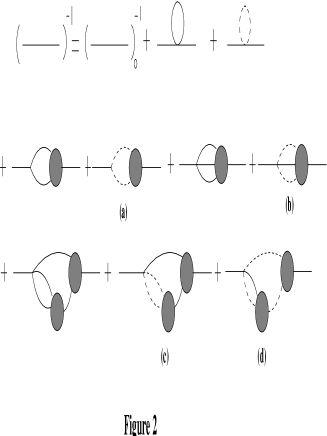
Figure 2: Schwinger-Dyson equations for the $\sigma$ two-point function

In these figures solid lines represent exact $\sigma$-propagators and dashed lines exact $\pi$-propagators( except the lines with subscript ‘0’ denoting tree level propagators ), and all blobs represent exact vertices.

We assume some infrared regulator like the external field H. Then $m_{\pi}$, the Goldstone boson mass is not zero and we can safely study the zero momentum behaviour of various graphs. The degree of infrared divergence is reflected by the leading $m_{\pi}$-dependence. Our input is that the exact pion propagator has the behaviour $(k^{2}-m_{\pi}^{2})^{-1}$ for $k\rightarrow 0$, i.e. we put in the information that the pion has a canonical behaviour in the infrared and study the consequences for the $\sigma$-propagator.Diagram 2(a) contributing to $\Gamma^{2}_{\sigma\sigma}$ would behave like $m_{\pi}^{d-4}$ if $\Gamma_{\sigma\pi\pi}$ were O(1) in the IR (and consequently the total $\Gamma^{2}_{\sigma\sigma}$ would also be O(1) due to the Ward identity (eqn 54)). This contribution is of order O(1) in the large-N count. Thus, either the IR-singular behaviour of 2(a) is cancelled by other diagrams in fig (2) or $\Gamma_{\sigma\pi\pi}$ must be at least as soft as $m_{\pi}^{4-d}$. Diagrams with potential IR-divergences are 2(b),2(c) and 2(d); apart from all of them being of O(1/N), none of them is as IR-singular as 2(a). Hence cancellation is ruled out and $\Gamma_{\sigma\pi\pi}$ must behave at least like $m_{\pi}^{4-d+\alpha}$ with $\alpha$-positive semidefinite. Consequently $\Gamma^{2}_{\sigma\sigma}$ must vanish as either $m_{\pi}^{2}$ or $m_{\pi}^{4-d+\alpha}$ whichever is dominanat.
While this proves conclusively that $\chi_{L}$ must diverge, we still need to restrict $\alpha$ further. It should be noted that $\Gamma^{2}_{\sigma\sigma}$ has terms of order $m_{\pi}^{0}$ and $O(1)$ in the large-N count. On the other hand $\Gamma^{2}_{\sigma\sigma}$ must vanish as some power of $m_{\pi}$. This is only possible if the $m_{\pi}^{0}$ terms are cancelled by such terms from the other diagrams. As all the diagrams except 2(a) are $O(1/N)$, generically this can only happen from the ultraviolet contributions to 2(a). Within $1/N$ perturbation theory at least, such cancellations are not possible in which case the $m_{\pi}^{0}$ terms must be generated in the infrared by 2(a) and this is possible only if $\alpha=0$. This completes the proof based on SD-equations.

7 Some Universal Features of Multipion Processes

We have thus established that the divergence of the longitudinal susceptibility is very general depending only on the goldstone phenomena. In fact, we have shown on very general grounds that the leading infrared behaviour of the longitudinal two-point function is completely universal.

Now we show that the same considerations lead to certain universal features of multipion scattering amplitudes. Such universal features were alluded to in Weinberg’s article [4]. Consider, for example, the expression (67) for the $\pi-\pi$ scattering amplitude at zero momentum. Eqn (74) can be recast as

$$f^{\prime} \sim H^{\frac{4-d}{2}}\ \ 2<d<4$$ (87)

$$\sim(lnH)^{-1}\ \ for\ \ d=4$$

Hence $4v^{3}f^{\prime}v^{2})>>H$ as $H\rightarrow 0$ and one has

$$A_{4\pi}=\frac{4i}{v^{3}}(H+\frac{H^{2}}{4v^{3}f^{"}(v^{2})}+\cdots)(\delta_{ij}\delta_{kl}+\cdots)$$ (88)

On recalling that in the absence of the infrared cut-off H, the scale that replaces $H$ is $E^{2}$, we recognise that the leading universal infrared behaviour $A_{4\pi}\sim E^{2}$ is indeed the well known result for soft pion scattering (usually derived in $d=4$). This universal behaviour does not depend on the space time dimensionality.

However (88)demonstrates that even the next to leading term is universal. The above considerations can be applied to multi-pion scatering amplitudes and one again finds the same universality of the first two terms. It is also clear from this paper that these results are non-perturbative in nature.

The presence of these non-analytic (in energy-momentum variables) terms in $d=4$ had been noted by Li and Pagels [7], the coefficients of which in the case of $\pi-\pi$ scattering had been calculated by Lehmann, and Lehmann and Trute [6] using unitarity. Weinberg showed that the application of renormalisation group can be used to show the universality of these logarithmic terms. He implicitly uses chiral symmetry. Though superficially it appears that the universality of the logarithmic terms is a one-loop result, careful reexamination of Weinberg’s demonstartion shows that it is an all-loop result.

In our approach, the origin of the universality of these subdominant logarithmic terms is directly related to universal divergence of the longitudinal susceptibility.

Our large-N derivation, which links the divergence of the $\chi_{L}$ to the special properties of the auxiliary field also demonstrates the universal features in a very straightforward manner.

The multipion scattering amplitudes in this case can be classified into three categories: a) those involving only $\lambda$ and $\pi$ propagators, and the $\lambda\pi^{2}$ vertices. For the scattering amplitude involving 2n pions (including initial and final states ),one needs $n-1~{}\lambda$ and $n-2~{}\pi$ propagators. Hence the IR-behaviour of all multipion amplitudes of this class is $\sim p^{2}$. b) Amplitudes involving one $n\lambda$ vertex and n $\lambda\pi^{2}$ vertices. The $n\lambda$-vertex scales like ${p^{2}}^{d/2-n}$. Hence this contribution to the amplitude scales like ${(p^{2})}^{d/2}$, which is less dominant than the behaviour a). Finally, there is the class c) which consists of amplitudes involving combinations of multi-$\lambda$ vertices with $m<n$.Their contribution can be seen to be even less dominant than b).

Because of the $k^{2}I(k^{2})$ factors in the denominators of the $\lambda$-propagator, one gets a universal correction factor $[1+\frac{k^{2}I(k^{2})}{v^{2}}]$ and the leading IR behaviour of these correction factors is the same in the linear and non-linear $\sigma$-models. This is precisely the same quantity that governs the universal divergence of $\chi_{L}$.

We now make a few geenral remarks about conventional chiral perturbation theory (ChPT) and compare it with our approach.

As we have already stated many times earlier, the leading IR behaviour of systems with Goldstone bosons is completely universal, and in the sector of Goldstone bosons only, is represented by the Lagrangian

$${\cal L}=\frac{1}{2}(\partial_{\mu}{\vec{\pi}})^{2}+\frac{1}{2f_{\pi}^{2}}\frac{({\vec{\pi}}\times\partial_{\mu}{\vec{\pi}})^{2}}{(1-\frac{{\vec{\pi}}^{2}}{f_{\pi}^{2}})^{2}}$$ (89)

This, following Weinberg, can be cast in the form

$${\cal L_{0}}=\frac{1}{2}(D_{\mu}{\vec{\pi}})^{2}$$ (90)

The validity of (89) is, however, strictly in the extreme infrared. One of the procedures adopted to extend (89 to regions beyond the extreme IR is the so-called chiral perturbation theory. In the form that is mostly practised, ChPT amounts to starting, for example, from a Lagrangian of the form

$${\cal L}={\cal L_{0}}+\frac{1}{2}(D_{\mu}\pi)^{2}+\frac{g_{4}^{(1)}}{2}(D_{\mu}\pi\cdot D^{\mu}\pi)^{2}+\frac{g_{4}^{(2)}}{2}(D_{\mu}\pi\cdot D_{\nu}\pi)(D_{\mu}\pi\cdot D_{\nu}\pi)+\cdots$$ (91)

Contrary to the attitude of the early days of effective Lagrangians, one now carries out loop calculations with Lagrangians of the type (90) and (91). Owing to perturbatie non-renormalisability of these lagrangians, one needs infinitely many counter terms to absorb the various resulting infinities.. However, to any any desired accuracy in the momenta involved, one needs only a finite number of counter terms. The structure of the resulting renormalised Lagrangian whose domain of validity is somewhat larger that that of (89) is that it is charaterised by a number of unknown parameters corresponding to the number of counteer terms used as well as certain universal parts independent of these unknown coefficients ($f_{\pi}$ is always treated as known). This is indeed the general structure argued by Weinberg.

Our analysis that the leading IR behaviour is governed by the Gaussian fixed point ${\cal G}_{N-1}$ points to a more efficient way of realising the results of ChPT. This suggestion was implicit in [4] also. This consists of perturbing the IR fixed point directly with the help of irrelevant operators. Their influence on all correlation functions can be directly computed by the use of the RG techniques. The ultraviolet degrees of freedom have no role to play in this scheme. This method will be applied to practical calculations of ChPT elsewhere.

8 Conclusions

In this paper we have emphasised that the quantum fluctuations of the Goldstone bosons have some drastic effects which are not encountered either in a tree level or loopwise analysis of the linear or the non-linear $\sigma$- models.Nevertheless,the leading infrared behaviour of the correlation functions again become identical in the linear and the non-linear versions.It is remarkable that the longitudinal fluctuations also become ‘massless’ as a consequence of the masslessness of the Goldstone bosons. We have exhibited the generality of this phenomenon giving three separate arguments based on i). Renormalization group flows, ii). Ward identities, iii). Schwinger-Dyson equations.

Heuristic derivations of the soft - pion theorems within the linear $\sigma$-model are based on the fact that $\sigma$-mass ($\chi_{L}^{-1}$) being non–zero, for all processes involving momenta much smaller than this mass the $\sigma$-propagator can be replaced by $m_{\sigma}^{-2}$. One may wonder whether the results of this paper would vitiate this and consequently the soft-pion theorems too. But as demonstrated in the sections on the large-N analysis as well as the one on Ward identities, the soft pion theorems are still valid. The deeper reason for this is, of course, the renormalisation group point of view according to which the leading IR-behaviour is controlled by the Gaussian fixed point.

As stressed sufficiently in this article, both the qualitative and quantitative aspects of the result,as far as the susceptibilities are concerned, were known in the literature from somewhat differing perspectives which were not general enough. What we have done here is to demonstrate the full generality of this result as well as extend the analysis to include the nonperturbative IR behaviour of correlation functions also. Despite the fact that the result concerning $\chi_{L}$ had appeared in the literature in different guises , its significance does not appear to have been well appreciated.

We emphasise that in the chiral limit the ‘sigma particle’ has a singular infrared behaviour (i.e. logarithmic divergence) even in four dimensions.

Independently of the space-time dimensions, the Goldstone bosons have canonical dimensions and decouple from each other and their logitudinal partners in the infrared.We pointed out that this can be understood from the Goldstone theorem, current algebra and PCAC on the one hand and the flow towards $O(N-1)$ Gaussian fixed point on the other hand. This latter point of view is very valuable because one can easily study the non-leading corrections to the infrared behaviour by standard renormalization group methods [8]. All effects of the microscopic theory could be parametrised in a few irrelevant and marginal operators around the $O(N-1)$ Gaussian fixed point and their effects computed. This approach provides a technically more efficient and conceptually simpler alternative to chiral perturbation theory, which focusses on the infrared divergence of the Goldstone bosons instead of the non-renormalizable ultraviolet divergences.

We showed that the leading $N$ approximation takes into account all the infrared behaviours accuratly, including that of the longitudinal fluctuations, in contrast to perturbation theory based on the linear or the non-linear $\sigma$- models.We developed a technique which allows explicit computation of the correlation functions even far away from the infrared region.This provides a useful non-perturbative technique for obtaining a qualitative understanding of the effects of fluctuations.

A convenient tool for understanding longitudinal susceptibility is the equation of state [8].In terms of the reduced variables $y=H/M^{\delta},x=t/M^{1/\beta}$,where M is the magnetisation, t the deviation from the critical temperature,and $\delta,\beta$ the standard exponents, the equation of state takes the universal form

$$y=f(x)$$ (92)

As H tends to zero, $x$ must tend to one of the roots of $f(x)$. With suitable normalisation this root (corresponding to spontaneous magnetization) can be arranged to be at $x=-1$.Now,the question of whether $\chi_{L}$ diverges or not can be answered by knowing the manner in which $f(x)$ approaches zero as $x$ approaches $-1$.If this approach is parametrised as

$$f(x)=(1+x)^{1+p}$$ (93)

where p is a positive semidefinite number, the behaviour of $\chi_{L}$ as H tends to zero is given by

$$\chi_{L}\sim H^{-p/(1+p)}$$ (94)

In the large-N expansion for arbitrary d (except d=4 where there are logarthmic modifications),the equation of state is

$$y=(1+x)^{\frac{2}{d-2}}$$ (95)

as can be proven using the euclidean version of eqn(52) of sec 4(see also [8]). As the exponent of $(1+x)$ is greater than 1 one concludes that the longitudinal susceptibility diverges for all $T<T_{c}$. Modulo the wavefunction renormalisation constant, $\chi_{L}$ is just $m_{\sigma}^{-2}$.

There are interesting consequences of this phenomena both for finite temperature QCD as well as QCD at zero temperature. In the case of the former, under the well argued scenario that this is a second order transition, Wilczek and Rajagopal [3] conclude that the transition must belong to the universality class of $d=3~{}~{}~{}O(4)$ magnet models. Then the general results of this paper become applicable.
In numerical simulations of the QCD chiral phase transition at finite temperature,the quantity that has been used to characterise the nature of the phase transition is the so-called $\Delta$-cumulant defined by [22]

$$\Delta={\partial ln\bar{\psi}\psi\over\partial lnm_{q}}$$ (96)

where $\bar{\psi}\psi$ is the chiral condensate and $m_{q}$ the current-quark mass.Thus

$$T>T_{c} ~{}~{}~{}~{}~{}~{}~{}~{}~{}\bar{\psi}\psi\sim m_{q}~{}~{}~{}~{}~{}~{}\Delta=1$$ (97)

$$T=T_{c} ~{}~{}~{}~{}~{}~{}~{}~{}~{}\bar{\psi}\psi\sim m_{q}^{1/\delta}~{}~{}~{}~{}~{}\Delta=1/\delta$$

Below $T_{c}$,but close to it, one should expect, on the basis of the considerations of this paper

$$T<T_{c}~{}~{}~{}~{}~{}~{}~{}~{}~{}\Delta\sim m_{q}^{1/2}$$ (98)

The same considerations apply to the spontaneously broken phase of zero temperature QCD. Here one should find

$$\Delta\sim m_{q}lnm_{q}$$ (99)

characterstic of Goldstone phenomena in four dimensions.
Of course, the arguments of Wilczek and Rajagopal that maps the problem to a classical stat mech problem in $d=3$ is valid exactly at $T_{c}$. But continuity would demand that at temperatures in the vicinity of $T_{c}$ too the effective dimensionality should be close to 3. Thus, the expectations based on eqs (97,98 and 99 ) are the correct ones. This should yield the experimentally interesting signal that for QCD at finite temperatures $T<T_{c}$, $\chi_{L}$ should smoothly go over from eqn (98) to eqn(99) as T is lowered.
Indeed, wherever there are Goldstone bosons, one should expect to see the singular behaviour of $\chi_{L}$. It is therefore somewhat disappointing that clear experimental signatures of this effect have not yet been found even for the classic ferromagnets.The lack of isotropy in most real life ferromagnets would make the experimental establishment of this effect a challenging one. An attempt to see this for ferromagnets has recently been made by [23]. They should have been looking for a $\chi_{L}\sim H^{-1/2}$ behaviour rather than $\chi_{L}\sim H^{-1/3}$. The fact that the behaviour of $\chi_{L}$ is ’super-universal’ in the sense that it depends only on dimension and the existence of Goldstone modes should be established in as many diverse experimental circumstances as possible. As Patashinsky and Pokrovsky [15] have pointed out, the effect should also be observable in the superfluid phase of He.Numerical simulations of the $O(N)$- models in three dimensions, performed in the ordered phase, should also establish this effect.
Kogut et al. [24] report a completely different behaviour and different exponents for the finite temperature chiral transition in QCD in comparison to [3]. In particular, Kogut et al. do not find the crucial softening of the longitudinal mode. More specifically,they argue that PCAC restricts the equation of state to be of the form

$$f(x)=(1+x)$$ (100)

There is a fallacy in their argument; PCAC implies the above form of the equation of state if and only if the longitudinal susceptibility is assumed to be finite. Only then a Taylor expansion around zero applied magnetic field is permissible.But our results about the divergence of $\chi_{L}$ imply that the assumption of a finite $\chi_{L}$ is incorrect. Once allowance is made for a diverging $\chi_{L}$, PCAC no longer places any restriction on the form of the equation of state. Also, Kogut et al. carry out their analysis in $d=4$ even at the critical temperature.

Acknowledgements
The main inspiration for this work came from the paper by Wilczek and Rajagopal. We have benefitted from discussions with many of our colleagues, in particular, V.Soni, G.Baskaran, Deepak Kumar, P.K. Mitter J.B. Zuber and E. Seiler.

References

- [1] For a review see, Aspects of Symmetry, S.Coleman (Cambridge Univ. Press(1985)).
- [2] For a review see, Current Algebra S.Adler and R.Dashen, A. Benjamin Inc. (1968)
- [3] F.Wilczek, Int.J.Mod.Phys.A7(1992) 3911; K.Rajagopal and F.Wilczek, Nucl.Phys. B399 (1993) 395.
- [4] S. Weinberg, Physica 96A (1979) 341.
- [5] For reviews see, H.Leutwyler,Recent Aspects of Quantum Fields,ed. H.Mitter and M.Gausterer, Lecture Notes in Physics 396(1991)1;Principles of Chiral Perturbation Theory, Preprint no BUTP-94/13, also published in Hadron Physics 94, 1-46; hep-ph/9406283.
- [6] H. Lehmann, Phys. Lett. B41, (1972) 529; H. Lehmann and H. Trute, Nucl. Phys. B52 (1973) 280;
- [7] L.-F. Li and H. Pagels, Phys. Rev. Lett. 26 (1971) 1204; ibid. 27 (1971) 1089; P. Langacker and H. Pagels Phys. Rev. D8 (1973) 4595.
- [8] See for instance, J.Zinn-Justin, Quantum Field Theory and Critical Phenomena, Clarendon Press, Oxford, 1989.
- [9] T. Holstein and H. Primakoff, Phys. Rev.58, 1098(1940).
- [10] D.J. Wallace and R.K.P. Zia, Phys. Rev. B12,5340(1975).
- [11] W.A.Bardeen, B.W.Lee and R.E.Schrock D14(1976)985.
- [12] S.Weinberg, Phys. Rev. Lett 18 188(1967)
- [13] T.H Berlin and M. Kac, Phys. Rev 86 (1952) 521; H.E. Stanley, Phys. Rev 176(1968)718.
- [14] A.Z. Patashinsky, V.L. Pokrovsky, Sov Phys JETP 37,733(1973). See also, V.G. Vaks, A.I. Larkin and S.I. Pikin, Sov. Phys. JETP 26,647(1968); M.E. Fisher, M.N. Barber and D. Jasnow, Phys. Rev A8,1111(1973).
- [15] A.Z. Patashinsky, V.L. Pokrovsky,Fluctuation Theory of Phase Transition, Moscow, Nauka 2075:Pergamon, London.
- [16] E. Brezin, D.J. Wallace and K.G. Wilson, Phys. Rev. B7, 232(1973).
-
[17]
F.Dunlop and C.M.Newman, Commun. Math. Phys.44
(1975)223.
J. Lebowitz and O. Penrose (as communicated to Dunlop and Newman) - [18] E. Brezin and J.Zinn-Justin, Phys. Rev. Lett.36 (1976) 691.
- [19] Private communication by J.Zinn-Justin.
- [20] D.J. Amit, Field Theory, the Renormalisation Group and Critical Phenomena, World Scientific, 1980.
- [21] I.Ya.Aref’eva,E.R.Nissimov and S.J.Pacheva Commun. Math. Phys. 71 (1980) 213; I.Ya.Aref’eva,S.I.Azakov, Nucl.Phys. B162 (1980) 298.
-
[22]
F. Karsch, Phys. Rev. D49 (1994) 3791.
F. Karsch and E. Laerman, Phys. Rev. D50(1994) 6954.
C. de Tar, Nucl. Phys. Proc. Suppl. 42 (1995) 457.
- [23] Koetzler and Muschke, Phys Rev B34(1986)3543;
- [24] A.Kocic, J.B.Kogut and M-P Lombardo, Nuc Phys B413(1994) 503.