UCB-PTH-95/02
hep-th/9501144 LBL-36686
CERN-TH.95/2
CPTH-A342.0195

Irrational Conformal Field Theory

M.B. Halpern¹ , E. Kiritsis² , N.A. Obers³ , K. Clubok¹ 1. Department of Physics, University of California and
Theoretical Physics Group, Lawrence Berkeley Laboratory
Berkeley, California 94720, USA 2. Theory Division, CERN, CH-1211
Geneva 23, SWITZERLAND 3. Centre de Physique Théorique
Ecole Polytechnique, F-91128 Palaiseau, FRANCE

This is a review of irrational conformal field theory, which includes rational conformal field theory as a small subspace. Central topics of the review include the Virasoro master equation, its solutions and the dynamics of irrational conformal field theory. Discussion of the dynamics includes the generalized Knizhnik-Zamolodchikov equations on the sphere, the corresponding heat-like systems on the torus and the generic world-sheet action of irrational conformal field theory.

Introduction

This is a review of irrational conformal theory, a subject which has grown from the discovery [91, 144, 94] of unitary conformal field theories (CFTs) with irrational central charge.

More precisely, irrational conformal field theory (ICFT) is defined to include all conformal field theories, and, in particular, ICFT includes rational conformal field theory (RCFT)

$$\mbox{ICFT}\;\;\;\supset\supset\;\;\;\mbox{RCFT}$$

as a very small subspace (see Fig.1).

The central tool in the study of ICFT is the general affine-Virasoro construction [91, 144],

$$T=L^{ab}\hbox{ }^{*}_{*}J_{a}J_{b}\hbox{ }^{*}_{*}$$

where $T$ is a conformal stress tensor and $J_{a}$, $a=1\ldots$dim$\,g$ are the currents of a general affine Lie algebra. The matrix $L^{ab}$ is called the inverse inertia tensor of the ICFT, in analogy with the spinning top.

The Virasoro condition on $T$ is summarized by the Virasoro master equation (VME), which is a set of quadratic equations for the inverse inertia tensor. The solution space of the VME is called affine-Virasoro space. This space contains the conventional RCFTs (which include the affine-Sugawara and coset constructions) and a vast array of new, generically-irrational conformal field theories.

Generic irrationality of the central charge (even on positive integer level of affine compact Lie algebras) is a simple consequence of the quadratic nature of the VME, and, similarly, it is believed that the space of all unitary theories is dominated by irrational central charge. Many candidates for new unitary RCFTs, beyond the conventional RCFTs, have also been found.

A coarse-grained picture of affine-Virasoro space is obtained by thinking in terms of the symmetry of the inverse inertia tensor in the spinning top analogy: The conventional RCFTs are very special cases of relatively high symmetry, while the generic ICFT is completely asymmetric.

Many exact unitary solutions with irrational central charge have been found, beginning with the solutions of Ref. [94]. More generally, the conformal field theories of affine-Virasoro space have been partially classified, using graph theory [97, 93] and generalized graph theory [102]. Remarkably, all the ICFTs so far classified are unitary on positive integer level of the compact affine algebras.

This review is presented in three parts,

I.  The General Affine-Virasoro Construction

II.  Affine-Virasoro Spaceuuuuuuuuuuuuuuuu

III.  The Dynamics of ICFTuuuuuuuuuuuuuuu

which reflect the major stages in the development of ICFT.

Figure 1: RCFTs are rare in the space of all ICFTs.

$\bullet$ Part I. The first part includes a discussion of the VME, and the associated N=1 and N=2 superconformal master equations [73]. General constructions satisfying the $W_{3}$ algebra are also reviewed. This part also includes the geometric reformulation [108] of the VME as an Einstein equation on the group manifold, the exact C-function [74] on affine-Virasoro space and the possibility [130] that conformal field theories may exist which are more general than those of the VME.

$\bullet$ Part II. The second part discusses the solution space of the master equations in further detail, including the known exact unitary solutions with irrational central charge. The high-level expansion [96] of the master equations and the partial classification of affine-Virasoro space by graph theory are also reviewed here. The partial classification by graph theory involves a new connection between groups and graphs, called generalized graph theory on Lie $g$ [102], which may be of interest in mathematics.

$\bullet$ Part III. In the third part we discuss the dynamics of ICFT, which includes the generalized Knizhnik-Zamolodchikov equations [103-105] on the sphere and the corresponding heat-like systems [106] on the torus. These equations describe the correlators and characters of the general ICFT, including a new description of the coset constructions on the sphere and the torus. As applications, we review the associated new results for coset constructions and the more general high-level solutions for the generic ICFT on simple $g$. This part also contains a review of the generic world-sheet action [109, 28] of ICFT, including a speculation on its relation to $\sigma$-models.

Three short reviews of ICFT [87-89] have also appeared, which follow the same stages in the development of the subject.

ICFT is not a finished product. Here is a list of some of the central outstanding problems.

1. Classification. Large as they are, the graph theories classify only small regions of affine-Virasoro space (see Section 7). A complete classification is an important open problem.

2. Correlators. Although the high-level correlators of ICFT are known (see Section 11), it is an important open problem to obtain the finite-level correlators of any of the exactly known unitary theories with irrational central charge.

3. Other approaches to ICFT. Beyond the approach reviewed here, complementary approaches to ICFT are an important open problem. In this connection, we mention the promising directions through non-compact coset constructions [42, 21] and through subfactors [114, 152] in mathematics.

Other open problems are discussed as they arise in the text.

Part I The General Affine-Virasoro Construction

1 Affine Lie Algebras and the Conventional Affine-Virasoro Constructions

1.1 Affine Lie Algebra

Mathematically an affine Lie algebra [115, 143, 18] $\hat{g}$ is the loop algebra of a finite dimensional Lie algebra $g$ (maps from $S^{1}\to g$) with a central extension. The generators of the affine algebra can be represented as $J_{a}(\theta)$, $a=1\ldots$dim$\,g$ with $\theta$ the angle parametrizing $S^{1}$. The generators $J_{a}(\theta)$ are often called the currents because they are Noether currents in field-theoretic realizations of affine algebras. The Fourier modes $J_{a}(m)$, $m\in{\mathchoice{\hbox{$\tensans\textstyle Z\kern-3.99994ptZ$}}{\hbox{$\tensans\textstyle Z\kern-3.99994ptZ$}}{\hbox{$\tensans\scriptstyle Z\kern-2.10002ptZ$}}{\hbox{$\tensans\scriptscriptstyle Z\kern-0.99998ptZ$}}}$, of the currents are often used as a convenient basis. See Ref. [117] for a detailed discussion of affine Lie algebras in mathematics.

The most general untwisted affine Lie algebra $\hat{g}$ is

$$[J_{a}(m),J_{b}(n)]=i{f_{ab}}^{c}J_{c}(m+n)+mG_{ab}\delta_{m+n,0}\,\,\,,\,\,\,\;\;m,n\in{\mathchoice{\hbox{$\tensans\textstyle Z\kern-3.99994ptZ$}}{\hbox{$\tensans\textstyle Z\kern-3.99994ptZ$}}{\hbox{$\tensans\scriptstyle Z\kern-2.10002ptZ$}}{\hbox{$\tensans\scriptscriptstyle Z\kern-0.99998ptZ$}}}$$ (1.1.1)

where $a,b,c=1\ldots$dim $g$ and ${f_{ab}}^{c}$ and $G_{ab}$ are respectively the structure constants and generalized Killing metric of $g$, not necessarily compact or semisimple. The zero modes $J_{a}(0)$ of the affine algebra satisfy the Lie algebra of $g$.

The generalized Killing metric $G_{ab}$ satisfies the conditions,

$G_{ab}$ is symmetric

${f_{ab}}^{d}G_{dc}$ is totally antisymmetric.

For non-semisimple algebras the generalized metric is not limited to the Killing metric of the Lie algebra [146]. For semisimple algebras $g=\oplus_{I}g_{I}$, the generalized metric can be written as

$$G_{ab}=\oplus_{I}k_{I}\eta^{I}_{ab}$$ (1.1.2)

where $\eta^{I}_{ab}$ is the Killing metric of $g_{I}$. Each coefficient $k_{I}$ is related to the (invariant) level $x_{I}$ of the affine algebra by

$$x_{I}=2k_{I}/\psi_{I}^{2}$$ (1.1.3)

where $x_{I}$ is independent of the scale of the highest root $\psi_{I}$. Level $x$ of affine Lie $g$ is often denoted by $g_{x}$.

Unitarity of the representations of compact affine algebras requires the level to be a non-negative integer. Other important numbers are the dual Coxeter number $\tilde{h}_{g}$ of $g$ and the (invariant) quadratic Casimir operators,

$$\qquad\qquad{\tilde{h}}_{I}=Q_{I}/\psi_{I}^{2}\;\;,\;\;{f_{ac}}^{d}{f_{bd}}^{c}=-\oplus_{I}Q_{I}\eta^{I}_{ab}\qquad\qquad$$ (1.1.4a)

$$\qquad{\cal I}({\cal T}^{I})=Q({\cal T}^{I})/\psi_{I}^{2}\;\;\;,\;\;\;{({\cal T}_{a}^{I}\eta^{ab}_{I}{\cal T}_{b}^{I})_{J}}^{K}={\delta_{J}}^{K}Q({\cal T}^{I})\qquad$$ (1.1.4b)

$$\qquad\qquad{\cal T}=\oplus_{I}{\cal T}^{I}\;\;\;,\;\;\;J,K=1\ldots\dim{\cal T}\qquad\qquad$$ (1.1.4c)

where ${\cal T}^{I}$ is a matrix irreducible representation (irrep) of $g_{I}$.

Affine modules or highest weight representations of $\hat{g}$ are constructed as Verma modules. The raising operators are $J_{a}(n\geq 1)$ and the raising operators $J_{a}(0)$, $a\in\Phi_{+}$ of the positive roots. A highest weight state $|R_{\cal T}\rangle$ is annihilated by the raising operators and these states are classified by the highest weights of irreps ${\cal T}$ of $g$. The highest weight representation corresponding to ${\cal T}$ is generated by the action of the lowering operators on the highest weight state.

In physics it is convenient to consider the collection of states $|R_{\cal T}\rangle^{J}$, $J=1\ldots$dim$\,{\cal T}$, called the affine primary states, which are generated by the action of the zero modes of the algebra on the highest weight state. Thus, the affine-primary states satisfy

$$J_{a}(m\geq 0)|R_{\cal T}\rangle^{J}=\delta_{m,0}|R_{\cal T}\rangle^{K}{({\cal T}_{a})_{K}}^{J}$$ (1.1.5)

where ${\cal T}$ is the corresponding matrix irrep of $g$. The other states in the affine module are generated by the action of the negative modes $J_{a}(m\leq 0)$ of the currents on the affine primary states.

A special representation of $\hat{g}$ is the one corresponding to the trivial or 1-dimensional representation of $g$. We will denote its affine primary state by $|0\rangle$ and call it the affine vacuum, since it is the ground state in unitary field-theoretic realizations of $\hat{g}$.

Affine Lie algebras are realized in quantum field theory as algebras of local currents. The local form of the currents is

$$J_{a}(z)=\sum_{m\in{\mathchoice{\hbox{$\tensans\textstyle Z\kern-3.99994ptZ$}}{\hbox{$\tensans\textstyle Z\kern-3.99994ptZ$}}{\hbox{$\tensans\scriptstyle Z\kern-2.10002ptZ$}}{\hbox{$\tensans\scriptscriptstyle Z\kern-0.99998ptZ$}}}}{J_{a}(m)\over z^{m+1}}$$ (1.1.6)

and the operator product expansion (OPE) of the currents,

$$J_{a}(z)J_{a}(w)={G_{ab}\over(z-w)^{2}}+i{f_{ab}}^{c}{J_{c}(w)\over(z-w)}+{\rm reg.}$$ (1.1.7)

is equivalent to the mode algebra (1.1.1). We will also need the affine-primary fields,

$$J_{a}(z)R^{J}_{g}({\cal T},w)={R^{K}_{g}({\cal T},w)\over(z-w)}{({\cal T}_{a})_{K}}^{J}+{\rm reg.}$$ (1.1.8a)

$$R^{J}_{g}({\cal T},0)|0\rangle=|R_{\cal T}\rangle^{J}$$ (1.1.8b)

which are the interpolating fields of the affine-primary states.

1.2 Virasoro Algebra

The Virasoro algebra is [178],

$$[L(m),L(n)]=(m-n)L(m+n)+{c\over 12}m(m^{2}-1)\delta_{m+n,0}$$ (1.2.1a)

$$T(z)T(w)={c/2\over(z-w)^{4}}+{2T(w)\over(z-w)^{2}}+{\partial_{w}T(w)\over(z-w)}+{\rm reg.}$$ (1.2.1b)

$$T(z)=\sum_{m\in{\mathchoice{\hbox{$\tensans\textstyle Z\kern-3.99994ptZ$}}{\hbox{$\tensans\textstyle Z\kern-3.99994ptZ$}}{\hbox{$\tensans\scriptstyle Z\kern-2.10002ptZ$}}{\hbox{$\tensans\scriptscriptstyle Z\kern-0.99998ptZ$}}}}{L(m)\over z^{m+2}}$$ (1.2.1c)

where $T$ is called the stress tensor and $c$ is called the central charge. The central term was first observed by Weis [179]. A Virasoro primary field $\Phi_{\Delta}$ of conformal weight $\Delta$ satisfies

$$T(z)\Phi_{\Delta}(w)=\Delta{\Phi_{\Delta}(w)\over(z-w)^{2}}+{\partial\Phi_{\Delta}(w)\over(z-w)}+{\rm reg.}$$ (1.2.2a)

$$\Phi_{\Delta}(0)|0\rangle=|\Phi_{\Delta}\rangle$$ (1.2.2b)

$$L(m\geq 0)|\Phi_{\Delta}\rangle=\delta_{m,0}\Delta|\Phi_{\Delta}\rangle$$ (1.2.2c)

where $|\Phi_{\Delta}\rangle$ is a Virasoro primary state and $|0\rangle$ is the $SL(2,{\rm I\!R})$-invariant ground state with $\Delta=0$. See Ref. [23] for further discussion of the foundations of conformal field theory.

The affine-Virasoro constructions are Virasoro operators built from the currents of affine Lie algebra, and $|0\rangle$ is the affine vacuum in this case.

1.3 Affine-Sugawara constructions

The simplest affine-Virasoro constructions generalize the notion of quadratic Casimir operators in finite Lie algebras. These operators are the affine-Sugawara constructions [18, 83, 129, 162] on semisimple $g$, which read

$$L_{g}(m)=L^{ab}_{g}\sum_{n\in{\mathchoice{\hbox{$\tensans\textstyle Z\kern-3.99994ptZ$}}{\hbox{$\tensans\textstyle Z\kern-3.99994ptZ$}}{\hbox{$\tensans\scriptstyle Z\kern-2.10002ptZ$}}{\hbox{$\tensans\scriptscriptstyle Z\kern-0.99998ptZ$}}}}\hbox{ }^{*}_{*}J_{a}(m-n)J_{b}(n)\hbox{ }^{*}_{*}$$ (1.3.1a)

$$T_{g}(z)=L^{ab}_{g}\hbox{ }^{*}_{*}J_{a}(z)J_{b}(z)\hbox{ }^{*}_{*}$$ (1.3.1b)

$$L_{g}^{ab}=\oplus_{I}{\eta_{I}^{ab}\over 2k_{I}+Q_{I}}\;\;\;,\;\;\;c_{g}=\sum_{I}{x_{I}{\rm dim}\,g_{I}\over x_{I}+{\tilde{h}}_{I}}$$ (1.3.1c)

where $\eta_{I}^{ab}$ is the inverse Killing metric of $g_{I}$. The normal-ordering symbol $\hbox{ }^{*}_{*}\hbox{ }^{*}_{*}$ means that negative modes of the currents are on the left.

Under the affine-Sugawara construction, the currents and the affine primary fields are Virasoro primary fields,

$$T_{g}(z)J_{a}(w)={J_{a}(w)\over(z-w)^{2}}+{\partial_{w}J_{a}(w)\over(z-w)}+{\rm reg.}$$ (1.3.2a)

$$T_{g}(z)R_{g}^{J}({\cal T},w)=\Delta_{g}({\cal T}){R_{g}^{J}({\cal T},w)\over(z-w)^{2}}+{\partial_{w}R_{g}^{J}({\cal T},w)\over(z-w)}+{\rm reg.}$$ (1.3.2b)

$$\Delta_{g}({\cal T})=\sum_{I}{{\cal I}({\cal T}^{I})\over x_{I}+\tilde{h}_{I}}$$ (1.3.2c)

with conformal weights one and $\Delta_{g}({\cal T})$ respectively. In (1.3.2c), ${\cal I}({\cal T})$ is the quadratic Casimir operator (1.1.4b).

The affine-Sugawara constructions are realized field-theoretically in the WZW models [148, 181], which are reviewed in Section 14.3.

1.4 Coset constructions

The next simplest affine-Virasoro constructions are the $g/h$ coset constructions [18, 83, 75].

When $h\subset g$ is a subalgebra of $g$, the stress tensor of the $g/h$ coset construction is

$$T_{g/h}(z)=T_{g}(z)-T_{h}(z)=L^{ab}_{g/h}\hbox{ }^{*}_{*}J_{a}(z)J_{b}(z)\hbox{ }^{*}_{*}$$ (1.4.1a)

$$L^{ab}_{g/h}=L_{g}^{ab}-L_{h}^{ab}\;\;\;,\;\;\;c_{g/h}=c_{g}-c_{h}$$ (1.4.1b)

where $T_{g}$ and $T_{h}$ are the stress tensors of the affine-Sugawara construction on $g$ and $h$. The coset stress tensor commutes with the $\hat{h}$ current algebra and the affine-Sugawara construction on $h$,

$$T_{g/h}(z)J_{A}(w)={\rm reg.}\;\;\;\;A=1\ldots{\rm dim}\,h$$ (1.4.2a)

$$T_{g/h}(z)T_{h}(w)={\rm reg.}\;\;.$$ (1.4.2b)

The commutativity of the stress tensors implies that, for each $g/h$, the affine-Sugawara construction $T_{g}=T_{g/h}+T_{h}$ is a tensor product CFT, formed by tensoring the coset CFT with the CFT on $h$.

Coset constructions are realized field-theoretically as gauged WZW models [19, 67, 68, 122, 123].

Appendix: History of Affine Lie Algebra and the Appendix: Affine-Virasoro Constructions.

Early development of affine Lie algebra and the affine-Virasoro constructions followed independent lines in mathematics and physics.

1. Affine Lie algebra. Affine Lie algebra, or current algebra on the circle, was discovered independently in mathematics [115, 143] and physics [18].

In mathematics, the affine algebras were introduced as natural generalizations of finite dimensional Lie algebras, while in physics the affine algebras were introduced by example, in order to describe current-algebraic spin and internal symmetry on the string. The examples in physics included the affine central extension some years before it was recognized in mathematics.

Affine Lie algebras are also known as centrally-extended loop algebras. They comprise a special case of the more general system known as Kač-Moody algebra [115, 143], which also includes the hyperbolic algebras.

2. World-sheet fermions. World-sheet fermions were given independently in [18] and [156], which describe the (Weyl) half-integer moded and (Majorana-Weyl) integer moded cases respectively. Half-integer moded Majorana-Weyl fermions were introduced later in [147]. World-sheet fermions played a central role in the early representation theory of affine Lie algebras [18] and superconformal symmetry [156, 147].

3. Representations of affine Lie algebras. The first concrete realization [18] of affine Lie algebra was untwisted $SU(3)_{1}$. This realization followed the quark model [69] to construct the level-one currents from world-sheet fermions in the $3$ and $\bar{3}$ of $SU(3)$. Other fermionic realizations were given on orthogonal groups in [18, 83].

The vertex operator constructions of affine Lie algebra began in [84, 85, 11], which gave the construction of untwisted $SU(n)_{1}$ from compactified spatial dimensions. This work extended the Coleman-Mandelstam bosonization of a single fermion on the line [35, 137] to the bosonization of many fermions on the circle, and hence, through the fermionic realizations, to the bosonization of the affine currents. Technically, the central ingredients in this construction were the Klein transformations [133] or cocycles which are necessary for many fermions, and the recognition of the structural analogy between the string vertex operator [65] and Mandelstam’s bosonized fermion on the line.

Twisted scalar fields were first studied in [107, 167] and twisted vertex operators were introduced in [36].

Concrete realizations of affine Lie algebra came later in mathematics, where the first realization [135] was the vertex operator construction of twisted $SU(2)_{1}$. The untwisted vertex operator construction of $SU(n)_{1}$ in physics was also generalized [62, 161] to level one of simply laced $g$.

The vertex operator construction plays a central role in string theory as the internal symmetry of the heterotic string [82].

4. Affine-Sugawara constructions. The simplest set of affine-Virasoro constructions are the affine-Sugawara constructions, on the currents of affine Lie algebra. (Sugawara’s model [175, 174] was in four dimensions on a different algebra.) The first examples of affine-Sugawara constructions were given in [18, 83], using the fermionic representations of the affine algebra. The affine-Sugawara constructions were later generalized in [129, 162], and the corresponding WZW action was given in [148, 181].

5. Coset constructions. The next set of affine-Virasoro constructions were the $g/h$ coset constructions. The first examples of coset constructions were given implicitly in [18] and explicitly in [83]. They were later generalized in [75] and the corresponding gauged WZW action was given in [19, 67, 68, 122, 123].

6. Beyond the coset constructions. Ref. [18] also gave another affine-Virasoro construction, the spin-orbit construction, which was more general than the affine-Sugawara and coset constructions. The spin-orbit construction provided a central motivation for the discovery of the Virasoro master equation [91, 144], which collects all possible affine-Virasoro constructions. An independent motivation was provided in Ref. [130], which considered general Virasoro constructions using arbitrary (2,0) operators.

Other historical developments in conformal field theory are noted, as they arise, in the introductory sections of the text.

2 The Virasoro Master Equation

2.1 Derivation of the Virasoro Master Equation

In Section 1 we reviewed the simplest affine-Virasoro constructions, that is, the affine-Sugawara constructions and coset constructions. In this section, we discuss the general affine-Virasoro construction [91, 144],

$$T=L^{ab}\hbox{ }^{*}_{*}J_{a}J_{b}\hbox{ }^{*}_{*}$$ (2.1.1)

where $J_{a},a=1\ldots\dim g$ are the currents of affine $g$ and $L^{ab}=L^{ba}$ is called the inverse inertia tensor in analogy with the spinning top.

To set up the construction, one first defines the normal-ordered current bilinears via the current-current OPE,

$$J_{a}(z)J_{b}(w)={G_{ab}\over(z-w)^{2}}+i{f_{ab}}^{c}[{1\over z-w}+{1\over 2}\partial_{w}+{1\over 6}(z-w)\partial_{w}^{2}]J_{c}(w)\hskip 85.35826pt$$

$$\hskip 42.67912pt+[1+{1\over 2}(z-w)\partial_{w}]T_{ab}(w)+(z-w)X_{ab}(w)+{\cal O}[(z-w)^{2}]\;\;.$$ (2.1.2)

This expansion defines the spin-two composite operators

$$T_{ab}(z)=T_{ba}(z)=\hbox{ }^{*}_{*}J_{a}J_{b}\hbox{ }^{*}_{*}$$ (2.1.3)

and the spin-three operators $X_{ab}(z)=-X_{ba}(z)$, both operators being quasiprimary with respect to the affine-Sugawara construction on $g$. The two-point functions of $T_{ab}$ and $X_{ab}$,

$$\langle T_{ab}(z)T_{cd}(w)\rangle={P_{ab,cd}\over(z-w)^{4}}\,\,\,,\,\,\,\langle X_{ab}(z)X_{cd}(w)\rangle={H_{ab,cd}\over(z-w)^{6}}$$ (2.1.4)

can be computed from (2.1.2), where

$$P_{ab,cd}=G_{a(c}G_{d)b}-{1\over 2}{f_{a(c}}^{e}{f_{d)b}}^{f}G_{ef}$$ (2.1.5)

and $H_{ab,cd}$ is given in [74]. For affine compact $g$, the matrix $P_{ab,cd}$ is non-negative when each level $x_{I}$ of the simple components $g_{I}$ is some positive integer.

The next step is to compute the $T_{ab}J_{c}$ OPE,

$$T_{ab}(z)J_{c}(w) = {M_{ab,c}}^{d}\left[{1\over(z-w)^{2}}+{1\over(z-w)}\partial_{w}+{1\over 2}\partial_{w}^{2}\right]J_{d}(w)$$ (2.1.6)

$$+{N_{ab,c}}^{de}\left[{1\over(z-w)}+{3\over 4}\partial_{w}\right]T_{de}(w)+W_{abc}(w)$$

$$+{K_{ab,c}}^{de}X_{de}(w)+{\cal O}(z-w)$$

where

$${M_{ab,c}}^{d}={\delta_{(a}}^{d}G_{b)c}+{1\over 2}{f_{e(a}}^{d}{f_{b)c}}^{e}\;\;\;,\;\;\;{N_{ab,c}}^{de}={i\over 2}{\delta_{(a}}^{(d}{f_{b)c}}^{e)}$$ (2.1.7)

and (2.1.6) serves as a definition of the spin-three quasiprimary composite operators $W_{abc}(z)$.

Finally one computes the OPE among the current bilinears $T_{ab}$,

$$T_{ab}(z)T_{cd}(w)={P_{ab,cd}\over(z-w)^{4}}+{R_{ab,cd}}^{ef}\left[{1\over(z-w)^{2}}+{1\over 2(z-w)}\partial_{w}\right]T_{ef}(w)\hskip 85.35826pt$$

$$\hskip 42.67912pt+{Q_{ab,cd}}^{e}\left[{1\over(z-w)^{3}}+{1\over 2(z-w)^{2}}\partial_{w}+{1\over 6(z-w)}\partial_{w}^{2}\right]J_{e}(w)$$

$$+{S_{ab,cd}}^{efg}{W_{efg}(w)\over(z-w)}+{U_{ab,cd}}^{ef}{X_{ef}(w)\over(z-w)}+{\rm reg.}\hskip 22.76228pt$$ (2.1.8)

where $Q$, $S$ and $U$ are antisymmetric under the interchange $(ab\leftrightarrow cd)$ while $R$ is symmetric. The expressions for $Q$, $R$ and $S$ are given in [91, 74] and $P_{ab,cd}$ is defined in (2.1.5).

We are now ready to answer the question: What are the conditions on the inverse inertia tensor so that $T(L)$ in (2.1.1) satisfies the Virasoro algebra?

Using (2.1.8), it is not difficult to see that $L^{ab}$ must satisfy a system of quadratic equations

$$2L^{ab}=L^{cd}L^{ef}R_{cd,ef}{}^{ab}\;\;\;,\;\;\;c=2L^{ab}L^{cd}P_{ab,cd}\;\;.$$ (2.1.9)

Using the form of $R$ in Ref. [91], eq.(2.1.9) gives the explicit form of the Virasoro master equation [91, 144],

$$L^{ab}=2L^{ac}G_{cd}L^{db}-L^{cd}L^{ef}{f_{ce}}^{a}{f_{df}}^{b}-L^{cd}{f_{ce}}^{f}{f_{df}}^{(a}L^{b)e}$$ (2.1.10a)

$$c=2G_{ab}L^{ab}$$ (2.1.10b)

which is often abbreviated as VME below. The linear form of the central charge in (2.1.10b) is obtained by using the VME.

In summary, for each solution $L^{ab}$ of the VME, one obtains a conformal stress tensor $T(L)=L^{ab}\hbox{ }^{*}_{*}J_{a}J_{b}\hbox{ }^{*}_{*}$ with central charge (2.1.10b).

A Feigin-Fuchs generalization

A more general Virasoro construction has also been considered, where the stress tensor contains terms linear in the first derivatives of the currents [91]

$$T=L^{ab}\hbox{ }^{*}_{*}J_{a}J_{b}\hbox{ }^{*}_{*}+D^{a}\partial J_{a}\;\;.$$ (2.1.11)

In this case, the Virasoro conditions are the generalized VME [91, 108],

$$L^{ab}=2L^{ac}G_{cd}L^{db}-L^{cd}L^{ef}{f_{ce}}^{a}{f_{df}}^{b}-L^{cd}{f_{ce}}^{f}{f_{df}}^{(a}L^{b)e}+i{f_{cd}}^{(a}L^{b)c}D^{d}$$ (2.1.12a)

$$D_{a}(2G^{ab}L_{be}+{f^{ab}}_{d}L_{bc}{f^{cd}}_{e})=D_{e}\;\;\;,\;\;\;c=2G_{ab}(L^{ab}-6D^{a}D^{b})$$ (2.1.12b)

which includes the Feigin-Fuchs constructions [51, 71, 56] and the more general c-changing linear deformations in [61].

Another generalization with terms linear in the currents [91],

$$L(m)=L^{ab}T_{ab}(m)+D^{a}J_{a}(m)+{1\over 2}G_{ab}D^{a}D^{b}\delta_{m,0}$$ (2.1.13a)

$$c=2G_{ab}L^{ab}$$ (2.1.13b)

is summarized by the VME and the eigenvalue condition on $D$ in (2.1.12b). This generalization includes the original example [18] of these constructions, and the more general c-fixed linear deformations (or inner-automorphic twists) in [61].

We also note that a class of affine-Virasoro constructions has been found using higher powers of the currents [79], but these constructions are automorphically equivalent to the quadratic constructions.

A geometric formulation of the VME

The VME has been identified [108] as an Einstein-like equation on the group manifold $G$.

The central components in this identification are the left-invariant Einstein metric $g_{ij}$ on $G$ and the left-right invariant affine-Sugawara metric $g_{ij}^{(g)}$,

$$g_{ij}={e_{i}}^{a}{e_{j}}^{b}L_{ab}\;\;,\;\;g_{ij}^{(g)}={e_{i}}^{a}{e_{j}}^{b}L^{g}_{ab}$$ (2.1.14)

where ${e_{i}}^{a}$ is the left-invariant vielbein on $G$ and $L_{ab}$ is the inertia tensor. Then the VME may be reexpressed as the Einstein system,

$$\hat{R}_{ij}+g_{ij}=g^{(g)}_{ij}\;\;,\;\;\hat{R}_{ij}\equiv R_{ij}-{1\over 2}\tau_{kl(i}{\tau_{j)}}^{kl}\;\;,\;\;c={\rm dim}\,g-4R$$ (2.1.15)

where $R_{ij}$ and $R$ are the Ricci tensor and curvature scalar of $g_{ij}$ and $\tau$ is the natural contorsion on $G$. In the case of the generalized VME (2.1.11), one obtains an Einstein-Maxwell system on the group manifold.

VME on non-semisimple algebras

We emphasize that the VME is valid on non-semisimple algebras. In this case, the Killing metric $\eta_{ab}$ of the algebra (in $G_{ab}=k\eta_{ab}$) is degenerate so the set of solutions of the VME will not include an analogue of the affine-Sugawara construction. However, there are non-degenerate invariant metrics $\hat{\eta}_{ab}$ on some non-semisimple Lie algebras [146] which allow the alternate choice $G_{ab}=k\hat{\eta}_{ab}$ in the VME on the same semisimple algebra. In this case, one obtains an analogue [146, 131, 166, 149, 141, 142, 59, 128, 132, 127] of the affine-Sugawara construction with [141, 59]

$$[(2k+Q)\eta]^{-1}\to[2k\hat{\eta}+Q\eta]^{-1}$$ (2.1.16)

in (1.3). Moreover, all the structure of the VME described below is valid in this case, including K-conjugation and the coset constructions [131, 164, 165, 166, 5].

2.2 Affine-Virasoro Space

2.2.1 Simple properties

The solution space of the VME is called affine-Virasoro space. Here are some simple properties of this space.

1. Affine-Sugawara constructions [18, 83, 181, 129]. The affine-Sugawara construction $L_{g}$,

$$L_{g}^{ab}=\oplus_{I}{\eta_{I}^{ab}\over 2k_{I}+Q_{I}}\,\,\,\;\;,\,\,\,\;\;c_{g}=\sum_{I}{x_{I}{\rm dim}\,g_{I}\over x_{I}+{\tilde{h}}_{I}}$$ (2.2.1)

is a solution of the VME for arbitrary level of any semisimple $g$ and similarly for $L_{h}$ when $h\subset g$.

2. K-conjugation [18, 83, 75, 130, 91]. K-conjugation covariance is one of the most important features of the VME, playing a major role in the structure of affine-Virasoro space and the dynamics of ICFT.

When $L$ is a solution of the master equation on $g$, then so is the K-conjugate partner $\tilde{L}$ of $L$,

$$\tilde{L}^{ab}=L^{ab}_{g}-L^{ab}\;\;\;,\;\;\;\tilde{c}=c_{g}-c$$ (2.2.2)

and the corresponding stress tensors $T\equiv T(L)$ and $\tilde{T}\equiv T(\tilde{L})$ form a commuting pair of Virasoro operators,

$$T(z)+\tilde{T}(z)=T_{g}(z)$$ (2.2.3a)

$$T(z)\tilde{T}(w)={\rm reg.}$$ (2.2.3b)

which add to the affine-Sugawara stress tensor $T_{g}$.

The decomposition $T_{g}=T+\tilde{T}$ strongly suggests that, for each K-conjugate pair $T$ and $\tilde{T}$, the affine-Sugawara construction is a tensor product CFT, formed by tensoring the conformal field theories of $T$ and $\tilde{T}$. In practice, one faces the inverse problem, namely the definition of the $T$ theory by modding out the $\tilde{T}$ theory and vice versa. In the operator approach to the dynamics of ICFT, this procedure is called factorization (see Part III). K-conjugation also plays a central role in the world-sheet action of ICFT (see Section 14).

3. Coset constructions [18, 83, 75]. K-conjugation generates new solutions from old. The simplest examples are the $g/h$ coset constructions,

$$\tilde{L}=L_{g/h}=L_{g}-L_{h}\;\;,\;\;\tilde{T}=T_{g/h}=T_{g}-T_{h}\;\;,\;\;\tilde{c}=c_{g/h}=c_{g}-c_{h}$$ (2.2.4)

which follow by K-conjugation from the subgroup construction $L_{h}$ on $h\subset g$.

4. Affine-Sugawara nests [182, 94]. Repeated K-conjugation on nested subalgebras $g\supset h_{1}\supset h_{2}\cdots\supset h_{n}$ gives the affine-Sugawara nests,

$$L_{g/h_{1}/\ldots/h_{n}}=L_{g}-L_{h_{1}/\ldots/h_{n}}=L_{g}+\sum_{j=1}^{n}(-1)^{j}L_{h_{j}}$$ (2.2.5a)

$$\qquad c_{g/h_{1}/\ldots/h_{n}}=c_{g}-c_{h_{1}/\ldots/h_{n}}=c_{g}+\sum_{j=1}^{n}(-1)^{j}c_{h_{j}}\qquad$$ (2.2.5b)

which include the affine-Sugawara and coset constructions as the simplest cases. In what follows, we refer to the cases with $n\geq 2$ as the higher affine-Sugawara nests.

The nest stress tensors in (2.2.1) may be rearranged as sums of mutually-commuting stress tensors of $g/h$ and $h$,

$$T_{g/h_{1}/\ldots/h_{2m+1}}=T_{g/h_{1}}+\sum_{i=1}^{m}T_{h_{2i}/h_{2i+1}}$$ (2.2.6a)

$$T_{g/h_{1}/\ldots/h_{2m}}=T_{g/h_{1}}+\sum_{i=1}^{m-1}T_{h_{2i}/h_{2i+1}}+T_{h_{2m}}$$ (2.2.6b)

so the conformal field theories of the higher affine-Sugawara nests are expected to be tensor-product field theories, formed by tensoring the indicated constructions on $h$ and $g/h$. This was established at the level of conformal blocks in Ref. [104].

5. Affine-Virasoro nests [94]. Repeated K-conjugation on nested subalgebras $g_{n}\supset\cdots\supset g_{1}\supset g$ also generates the affine-Virasoro nests,

$$T^{\#}_{g_{2m}/.../g_{1}/g}=\sum_{i=1}^{m}T_{g_{2i}/g_{2i-1}}+T^{\#}_{g}$$ (2.2.7a)

$$T^{\#}_{g_{2m+1}/.../g_{1}/g}=\sum_{i=1}^{m}T_{g_{2i+1}/g_{2i}}+T^{\#}_{g_{1}/g}$$ (2.2.7b)

with an arbitrary construction $T^{\#}_{g}$ on $g$ at the bottom of the nest. In (2.2.7b), $T^{\#}_{g_{1}/g}=T_{g_{1}}-T^{\#}_{g}$ is the K-conjugate partner of $T^{\#}_{g}$ on $g_{1}$. In parallel with the form (* ‣ 2.2.1) of the affine-Sugawara nests, we have written the affine-Virasoro nest stress tensors as sums of mutually-commuting stress tensors. As above, the commutativity of the component stress tensors strongly suggests that the affine-Virasoro nests are tensor-product theories of the indicated coset constructions with the constructions $T^{\#}_{g}$ and $T^{\#}_{g_{1}/g}$.

6. Irreducible constructions [94]. Affine-Virasoro space exhibits a two-dimensional structure, with affine-Virasoro nesting as the vertical direction ($g$ above $h$ when $g\supset h$). The horizontal direction is the set of all constructions at fixed $g$, which contains in particular the subset of $irreducible$ $constructions$ on $g$

$$\{L^{\rm irr}_{g}\}\,\,:\,\,(L^{\rm irr}_{g})_{(0)}=L_{g}\,\,,\,\,(L^{\rm irr}_{g})_{(1)}\,\,,\,\,(L^{\rm irr}_{g})_{(2)}\,\,,\,\,....$$ (2.2.8)

which are not obtainable by nesting from below. Among the irreducible constructions on $g$, only one, the affine-Sugawara construction $L_{g}$, is a conventional RCFT. All the rest of the irreducible constructions are new CFTs, called the $new$ $irreducible$ $constructions.$

The number of new irreducible constructions is very large on large group manifolds and the new irreducible constructions have been enumerated [97] in the graph theory ansatz on $SO(n)$ (see Section 8.1). The graph theory also indicates that, on large manifolds, the generic ICFT is a new irreducible construction.

7. Unitarity [64, 75, 94]. Unitary constructions $L(m)^{\dagger}=L(-m)$ on positive integer level of affine compact $g$ are easily recognizable. If in a specific basis the currents satisfy

$$J^{\dagger}_{a}(n)={\rho_{a}}^{b}J_{b}(-n)$$ (2.2.9)

then a unitary construction $L$ satisfies

$$(L^{ab})^{*}=L^{cd}{(\rho^{-1})_{c}}^{a}{(\rho^{-1})_{d}}^{b}\;\;.$$ (2.2.10)

In particular $L^{ab}=$real is sufficient for unitarity in any Cartesian basis.

Unitarity guarantees that $c(L)\geq 0$, and K-conjugate partners of unitary constructions are also unitary with $c(\tilde{L})\geq 0$. The double inequality

$$0\leq c(L)\leq c_{g}$$ (2.2.11)

follows for all unitary Virasoro constructions on affine compact $g$. Moreover, all unitary high-level central charges [94, 96] on simple compact $g$ are integer valued from 0 to dim$\,g$ (see Section 7.2.3).

It is also known [75] that all unitary Virasoro constructions satisfying $0\leq c(L)<1$ can be realized as $g/h$ coset constructions. It follows that all unitary affine-Virasoro constructions satisfying $c_{g}-1<c(L)\leq c_{g}$ are realizable as the K-conjugate partners $T_{h}$ of the coset constructions with central charge between 0 and 1. Moreover, all unitary solutions of the VME with high-level central charge 0 , 1 , dim$\,g-1$ and dim$\,g$ are known [96] on simple compact $g$ (see Section 7.2.3).

8. $SL(2,{\rm I\!R})$-invariance [91, 94, 74]. The affine vacuum $|0\rangle$ satisfies

$$J_{a}(m\geq 0)|0\rangle=T_{ab}(m\geq-1)|0\rangle=0$$ (2.2.12a)

$$X_{ab}(m\geq-2)|0\rangle=W_{abc}(m\geq-2)|0\rangle=0$$ (2.2.12b)

so that all the conformal field theories of affine-Virasoro space are $SL(2,{\rm I\!R})$-invariant with $L(m\geq-1)|0\rangle=0$.

9. Spectrum [94]. The operator $L(0)$ can be diagonalized level by level in the affine modules and all the eigenvalues (conformal weights) are real and positive semidefinite for unitary constructions.

As an example, consider the $L^{ab}$-broken affine primary states

$$|R_{\cal T}\rangle^{\alpha}=|R_{\cal T}\rangle^{J}{\xi_{J}}^{\alpha}\;\;\;,\;\;\;\alpha=1\ldots{\rm dim}\,{\cal T}$$ (2.2.13a)

$$\qquad L^{ab}{({\cal T}_{a}{\cal T}_{b})_{J}}^{K}{\xi_{K}}^{\alpha}=\Delta_{\alpha}({\cal T}){\xi_{J}}^{\alpha}\qquad$$ (2.2.13b)

which diagonalize the conformal weight matrix $H=L^{ab}{\cal T}_{a}{\cal T}_{b}$. These states are Virasoro primary states of $T=L^{ab}\hbox{ }^{*}_{*}J_{a}J_{b}\hbox{ }^{*}_{*}$ with conformal weight $\Delta_{\alpha}({\cal T})$. See Section 9.2 for discussion of these states in a broader context.

There is an easy explicit demonstration of the consequences of unitarity in this case. When $L^{ab}$ is real on compact $g$, we have hermitian $H$, real $\Delta_{\alpha}({\cal T})$ and unitary $\xi$. Positivity of the space $\{|R_{\cal T}\rangle^{\alpha}\}$, and hence $\Delta_{\alpha}({\cal T})\geq 0$, follows from positivity of the unitary affine highest weight states.

10. Automorphically equivalent CFTs [108, 96, 97]. The elements $\omega\in{\rm Aut}\,g$ of the automorphism group of $g$ satisfy

$${f_{ab}}^{c}={\omega_{a}}^{d}{\omega_{b}}^{e}{(\omega^{-1})_{g}}^{c}{f_{de}}^{g}$$ (2.2.14a)

$$G_{ab}={\omega_{a}}^{c}{\omega_{b}}^{d}G_{cd}$$ (2.2.14b)

and (2.2.14b) may be written as

$${(\omega^{T})_{a}}^{b}\equiv G^{bc}{\omega_{c}}^{d}G_{da}={(\omega^{-1})_{a}}^{b}$$ (2.2.15)

so that $\omega$ is a (pseudo) orthogonal matrix which is an element of $SO(p,q)$, $p+q=$dim$\,g$ with metric $G_{ab}$. The automorphism group includes the outer automorphisms of $g$ and the inner automorphisms

$$g(\omega){\cal T}_{a}g^{-1}(\omega)={\omega_{a}}^{b}{\cal T}_{b}\;\,,\;\;\;g(\omega)\,\in\,G$$ (2.2.16)

where ${\cal T}$ is any matrix irrep of $g$.

The automorphisms of $g$ induce automorphically-equivalent CFTs in the VME as follows. The transformation

$${J^{\prime}_{a}}(m)={\omega_{a}}^{b}J_{b}(m)\,\,\,,\,\,\,\omega\,\in\,{\rm Aut}\,g$$ (2.2.17)

is an automorphism of the affine algebra (1.1.1), and $(L^{\prime})^{ab}$ defined by

$$(L^{\prime})^{ab}=L^{cd}{(\omega^{-1})_{c}}^{a}{(\omega^{-1})_{d}}^{b}$$ (2.2.18)

is an automorphically-equivalent solution of the VME when $L^{ab}$ is a solution.

Complete gauge-fixing or modding out by the automorphisms of $g$ [94, 97] is an important physical problem which has been completely solved only for the known graph theory units of ICFT (see Sections 7 and 8).

11. Generalized K-conjugation [93]. K-conjugation, which applies on all affine-Virasoro space, was described in item 2 of this list. A number of generalized K-conjugations also hold on the space of Lie $h$-invariant CFTs, which are those theories with a Lie symmetry $h\subset g$ (see Sections 6.1.1, 8.1.3, and 13.8). We mention in particular the case of $K_{g/h}$-conjugation,

$$(\tilde{L})_{g/h}=L_{g/h}-L\;\;,\;\;(\tilde{c})_{g/h}=c_{g/h}-c$$ (2.2.19)

whose action is conjugation through the coset stress tensor $T_{g/h}$ instead of $T_{g}$. This covariance holds in the subspace of the affine Lie-$h$ invariant CFTs, which is the set of all ICFTs with a local Lie symmetry. Similarly, generalized K-conjugations through the higher affine-Sugawara nests $T_{g/h_{1}/.../h_{n}}$ were discussed in [93].

2.2.2 A broader view

We collect here a number of more general features of affine-Virasoro space.

1. Level-families. Except for solutions at sporadic levels, the basic units of affine-Virasoro space are the conformal level-families $L^{ab}(k)$, which are essentially smooth functions of the affine level.

2. Counting. Because the VME has an equal number of equations and unknowns, one may count the generically-expected number $N(g)$ of conformal level-families on each $g$ [94],

$$N(g)=2^{{\rm dim}\,g({\rm dim}\,g-1)/2}\;\;.$$ (2.2.20)

These numbers are very large on large groups and, in particular, one finds that

$$N(SU(3))\simeq{1\over 4}{\rm billion}$$ (2.2.21)

so most conformal constructions await discovery,

$$\mbox{ICFT}\;\;\;\supset\supset\;\;\;\mbox{RCFT}\;\;.$$ (2.2.22)

The number of physically-distinct level-families on $g$ is less than (2.2.20) due to residual automorphisms [97], but the corrections are apparently negligible on large groups (see Section 8.1.2).

3. Generalized graph theories [97, 73, 98, 99, 101, 102, 93]. In the (partial) classification of the CFTs of affine-Virasoro space, one finds that the Virasoro master equation and the superconformal master equation generate generalized graph theories on Lie $g$, including conventional graph theory as a special case on the orthogonal groups. In the generalized graph theories, each generalized graph labels a conformal level-family.

This development began with conventional graph theory in [97], and the general case is axiomatized in [102]. We will return to this subject in Sections 7 and 8.

4. Unitary irrational central charge [94, 95, 160, 96-98, 101, 102, 93]. It is clear from the form of the master equation that the generic level-family has generically-irrational central charge, and, similarly, it is believed that the space of all unitary theories is dominated by irrational central charge. Indeed (on positive integer level of affine compact Lie algebras) unitary irrational central charge is generic for all the known exact level-families (see Section 6.3.1) and for all the level-families so far classified by the graph theories.

As an example, the value at level 5 of $SU(3)$ [96],

$$c\left((SU(3)_{5})^{\#}_{D(1)}\right)=2\left(1-{1\over\sqrt{61}}\right)\simeq 1.7439$$ (2.2.23)

is the lowest unitary irrational central charge yet observed. The nomenclature in (2.2.23) is discussed in Section 6.3.1.

2.2.3 Special categories

Beyond the generic level-families, we comment on a number of smaller categories seen so far in the VME.

1. Conventional RCFTs. In the development of ICFT, rational conformal field theory (RCFT) is defined as the small subspace of theories with rational central charge and rational conformal weights. The conventional RCFTs are defined as the set of affine-Sugawara nests, which includes the affine-Sugawara constructions, the coset constructions, and the higher affine-Sugawara nests.

2. New RCFTs [125, 34, 99, 100]. Beyond the conventional RCFTs, many candidates for new RCFTs have been found (see Sections 6.3.2 and 8.3).

3. CFTs with a symmetry $H\subset$ Aut $g$ [93]. Although most solutions $L^{ab}$ of the VME on $g$ have no symmetry (corresponding to a completely asymmetric spinning top), one sees a hierarchy of symmetry-breaking in the VME on $g$,

$${\rm Aut}\,g\to{\rm Lie}\,h\to H\to 1$$ (2.2.24)

where Aut $g$ is the maximal symmetry on $g$ and 1 is complete asymmetry. The $H$-invariant CFTs and the Lie $h$-invariant CFTs, which include the conventional RCFTs, are discussed in Sections 6.1.1, 8.1.3 and 13.8.

4. Quadratic deformations [144, 94, 145, 97, 24, 154, 73, 74, 98, 99, 159]. These are continuous manifolds of solutions in the VME, which occur at sporadic levels. The quadratic deformations are examples of quasi-rational CFTs, which have fixed rational central charge but generically-continuous conformal weights. There are no manifestly unitary constructions with continuously-varying central charge in the VME [74].

A set of sufficient conditions (see Section 3) has been found for the occurence of quadratic deformations [74], and other systematics are discussed in [94]. An explicit example of these constructions is reviewed in Section 6.2.2, and the names of all known exact quadratic deformations are listed in Section 6.3.2.

5. Self K-conjugate constructions [97, 98, 74]. In these constructions, the K-conjugate partners $\tilde{L}$ and $L$ are automorphically equivalent,

$${\tilde{L}}=\omega L\omega^{-1}\,\,\,\,\,\,\hbox{for some}\;\omega\,\in\,{\rm Aut}\,g$$ (2.2.25)

so that each construction in the pair has half affine-Sugawara central charge,

$$c={c_{g}\over 2}\;\;.$$ (2.2.26)

The self K-conjugate constructions are found on Lie group manifolds of even dimension. The first set of these constructions (see Section 8.1) was found on $SO(4n)$ and $SO(4n+1)$, where they are in one-to-one correspondence with the self-complementary graphs of graph theory. The names of all known exact self K-conjugate level-families are listed in Section 6.3.2, including examples on $SU(3)$ and $SU(5)$.

6. Self K_g/h-conjugate constructions [93]. These constructions are generalizations of the self K-conjugate constructions, in which K_g/h-conjugate pairs (see eq. (2.2.19)) are automorphically equivalent. In analogy with the self K-conjugate constructions, the self K_g/h-conjugate constructions have half coset central charge,

$$c={c_{g/h}\over 2}$$ (2.2.27)

and the names of the known exact level-families of this type are given in Section 6.3.2. It has been conjectured [93] that self-conjugate constructions exist for all the generalized K-conjugations described above.

2.3 More General Virasoro Constructions

The VME constructs Virasoro operators out of bilinears in affine currents. A presumably more general construction along these lines employs arbitrary (2,0) operators [130, 41].

Consider an initial conformal field theory which, in addition to its stress tensor $T_{\bullet}(z)$ with central charge $c_{\bullet}$, contains also a number of (2,0) operators $\Phi_{i}(z)$. These (2,0) operators can be either Virasoro primary under $T_{\bullet}$ or derivatives of (1,0) operators. We will not consider the second possibility, which leads to generalizations of the Feigin-Fuchs type [51, 71, 56]. The most general OPE among the operators $\Phi_{i}$, compatible with conformal invariance, is

$$\Phi_{i}(z)\Phi_{j}(w) = {\delta_{ij}\over(z-w)^{4}}+{4\over c_{\bullet}}\delta_{ij}{T_{\bullet}(w)\over(z-w)^{2}}+C_{ijk}{\Phi_{k}(w)\over(z-w)^{2}}$$ (2.3.1)

$$+{2\over c_{\bullet}}\delta_{ij}{\partial_{w}T_{\bullet}(w)\over(z-w)}+{1\over 2}C_{ijk}{\partial_{w}\Phi_{k}(w)\over(z-w)}+{\rm reg.}$$

where possible spin-one and spin-three terms have been suppressed because they do not contribute in the construction below. Eq.(2.3.1) also assumes the choice of an orthonormal basis for the $\Phi_{i}$. Associativity constrains the OPE coefficients $C_{ijk}$ to be completely symmetric in $i,j,k$.

One now considers a general linear combination of $T_{\bullet}$ and $\Phi_{i}$

$$T(z)=\lambda_{\bullet}T_{\bullet}(z)+\sum_{i=1}^{N}\lambda_{i}\Phi_{i}(z)$$ (2.3.2)

and demands that it satisfies the Virasoro algebra. Using the OPE (2.3.1), one obtains the following system of quadratic equations,

$$\sum_{i=1}^{N}(\lambda_{i})^{2}={1\over 2}\lambda_{\bullet}(1-\lambda_{\bullet})c_{\bullet}$$ (2.3.3a)

$$\sum_{i,j=1}^{N}C_{ijk}\lambda_{i}\lambda_{j}=2(1-2\lambda_{\bullet})\lambda_{k}\quad k=1,2,3\ldots N$$ (2.3.3b)

and the central charge $c$ of $T(z)$ is given by $c=\lambda_{\bullet}c_{\bullet}$. The K-conjugation covariance (2.2.2) seen in the VME is also a feature of the more general Virasoro construction: If $(\lambda_{\bullet},\lambda_{i})$ is a solution of (2.3.2), then one can verify that the K-conjugate partner $([1-\lambda_{\bullet}],-\lambda_{i})$ is also a solution. Moreover, the corresponding K-conjugate pair of stress tensors commute and sum to $T_{\bullet}$, as in the VME.

The more general Virasoro construction (MGVC) in (2.3.2) contains at least two representations,

$$T_{\bullet}=\left\{\matrix{T_{g}\cr T_{\rm free\,\,bosons}\cr}\right.\;\;\;\;\;,\;\;\;\;\;\;\left\{\Phi_{i}\right\}=\left\{\matrix{\hbox{ }^{*}_{*}J_{a}J_{b}\hbox{ }^{*}_{*}\cr\partial\phi^{i}\partial\phi^{j}\;\;\;,\;\;\;e^{i\vec{\alpha}\cdot\vec{\phi}}\;\;\;,\;\;\;\partial\phi^{i}e^{i\vec{\beta}\cdot\vec{\phi}}\cr}\right.$$ (2.3.4)

where the top line leads to the VME and the bottom line describes the Interacting Boson Models (IBMs) studied in [130, 46, 47, 124, 34]. Any affine-Virasoro construction can be bosonized into an IBM, so one sees the hierarchy of conformal constructions

$${\rm MGVC}\;\;\;\supset\;\;\;{\rm IBMs}\;\;\;\supset\;\;\;{\rm VME}\;\;.$$ (2.3.5)

We believe that the sets in this hierarchy are progressively larger towards the left, but this has not yet been demonstrated: The only known CFTs which may go beyond the VME are the N=2 IBMs discussed in Section 8.3.

3 The C-Function and a C-Theorem

In this section, the notion of affine-Virasoro space is extended to include all inverse inertia tensors $L^{ab}$, whether the operator $T(L)$ is Virasoro or not. On this space, there is an exact C-function and an associated flow which satisfies a C-theorem [74]. The notions of C-function and C-theorem in conformal field theory were introduced in Ref. [185].

This development begins with the following cubic function on affine-Virasoro space,

$$A(L)\equiv 2L^{ab}P_{ab,cd}(L^{cd}-2\beta^{ab}(L))$$ (3.1a)

$$P_{ab,cd}\equiv z^{4}\langle T_{ab}(z)T_{cd}(0)\rangle=G_{a(c}G_{d)b}-{1\over 2}{f_{a(c}}^{e}{f_{d)b}}^{f}G_{ef}$$ (3.1b)

$$\beta^{ab}(L)\equiv-L^{ab}+2L^{ac}G_{cd}L^{db}-L^{cd}L^{ef}{f_{ce}}^{a}{f_{df}}^{b}-L^{cd}{f_{ce}}^{f}{f_{df}}^{(a}L^{b)e}$$ (3.1c)

where $T_{ab}=\hbox{ }^{*}_{*}J_{a}J_{b}\hbox{ }^{*}_{*}$ and $P_{ab,cd}$ is the natural metric on the space. The function $A(L)$ is the correct action on affine-Virasoro space because the equation for its extrema

$${\partial A(L)\over\partial L^{ab}}=-12P_{ab,cd}\beta^{cd}(L)=0$$ (3.2)

is the Virasoro master equation. Moreover, the action is a C-function on affine-Virasoro space because

$$A(L)|_{\beta=0}=c(L)$$ (3.3)

is the central charge (2.1.10b) of the conformal stress tensor $T(L)$.

All the conformal field theories of the VME are fixed points of the associated flow,

$${\dot{L}}^{ab}=\beta^{ab}(L)$$ (3.4)

where overdot is derivative with respect to an auxiliary variable. This flow satisfies the C-theorem,

$${\dot{A}}(L)\leq 0$$ (3.5)

on positive integer level of affine compact $g$.

Ref. [74] discusses the flow equation (3.4) in further detail, including the flow near a fixed point and closed subflows. Closed subflows are associated to each consistent ansatz (see Section 6.1.1) of the VME. Of particular interest is the subflow in the ansatz $SO(n)_{diag}$, which is a flow on the space of graphs. Two other applications are discussed below.

1. Morse theory. The C-function is a Morse function [138] on affine-Virasoro space. Morse polynomials and the Witten index can be defined in the standard way for any closed subflow. In the case of the flow on the space of graphs, the Morse polynomials turn out to be well-known functions in graph enumeration.

2. Prediction of sporadic deformations. Using the flow equation, a set of sufficient conditions was derived for the occurence of a quadratic deformation (see Section 2.2.3) which, in this context, is a continuous family of fixed points:

If there are two level-families of the VME,

a) which are flow-connected at high level, and

b) whose central charges cross as the level is lowered,

then there is a continuous family of fixed points at the level where the central charges cross for the first time.

Concerning condition a), what must be checked in high-level perturbation theory is that there is a flow which starts from a small neighborhood of one of the level-families and ends at the other level-family. Condition b) was noted independently in [160]. This method was applied successfully in [74, 98, 159], leading to the exact forms of several new quadratic deformations in the VME.

Further discussion of quadratic deformations is found in Sections 6.2.2, 6.3.2 and Ref.  [94]

Speculation on the flow equation

The flow equation (3.4) bears a strong resemblance to the expected form of an exact renormalization group equation, but the flow equation cannot be the conventional renormalization group equation. The reason is that the conventional renormalization group analysis is restricted to Lorentz-invariant paths between CFTs, while the generic path of the flow equation is apparently non-relativistic.

More precisely, the flow equation, if indeed it corresponds to a renormalization group equation, is expected to run over the set of quantum field theories whose Hamiltonian,

$$H=L^{ab}\sum_{m\in{\mathchoice{\hbox{$\tensans\textstyle Z\kern-3.99994ptZ$}}{\hbox{$\tensans\textstyle Z\kern-3.99994ptZ$}}{\hbox{$\tensans\scriptstyle Z\kern-2.10002ptZ$}}{\hbox{$\tensans\scriptscriptstyle Z\kern-0.99998ptZ$}}}}\hbox{ }^{*}_{*}[J_{a}(-m)J_{b}(m)+\bar{J}_{a}(-m)\bar{J}_{b}(m)]\hbox{ }^{*}_{*}$$ (3.6)

is the natural extension [87] of the generic affine-Virasoro Hamiltonian (see Section 14.2) to arbitrary $L^{ab}$.

As noted in [87], the theories in this set are scale invariant (due to normal ordering) and the generic theory is non-relativistic. At a fixed point, where $L^{ab}$ satisfies the VME, Lorentz and conformal invariance are restored ($H=L(0)+\bar{L}(0)$) and the theory develops a spin-two gauge symmetry [109] due to K-conjugation. See Section 13 for further discussion of this Hamiltonian at the fixed points, including the corresponding world-sheet action of the generic ICFT.

The overall picture here may be formulated as a conjecture that the renormalization group equation of the large set of theories (3.6) is the flow equation (3.4). Moreover, all these theories (including the CFTs) may be integrable models because their spectrum is solvable level-by-level in the affine modules.

4 General Superconformal Constructions

Superconformal algebras play a special role in CFT and string theory. The simplest example is the N=1 superconformal algebra [156, 147] which contains in addition to the stress tensor an extra fermionic field (the supercurrent) with spin 3/2. This algebra is the gauge algebra of the superstring (see e.g. [81]). Consequently, the representations of the algebra are crucial in finding superstring ground states. Extended superconformal algebras also play an important role in superstring theory: N=2 superconformal symmetry [1, 2] is needed [10] to construct ground states of the heterotic string [82] with at least N=1 spacetime supersymmetry in four dimensions. If N=4 superconformal symmetry [2] is present then one obtains at least N=2 spacetime supersymmetry [9].

The N=1 and N=2 superconformal master equations, which collect the N=1 and N=2 superconformal solutions of the VME, were obtained by Giveon and three of the authors in Ref. [73]. In what follows we review both of these systems.

4.1 The N=1 Superconformal Master Equation

The N=1 superconformal algebra is [156, 147],

$$[L(m),L(n)]=(m-n)L(m+n)+\frac{c}{12}m(m^{2}-1)\delta_{m+n,0}$$ (4.1.1a)

$$\{G(r),G(s)\}=2L(r+s)+\frac{c}{3}(r^{2}-\frac{1}{4})\delta_{r+s,0}$$ (4.1.1b)

$$[L(m),G(r)]=(\frac{m}{2}-r)G(m+r)$$ (4.1.1c)

where $G(r)$ is the supercurrent, with $r\in{\mathchoice{\hbox{$\tensans\textstyle Z\kern-3.99994ptZ$}}{\hbox{$\tensans\textstyle Z\kern-3.99994ptZ$}}{\hbox{$\tensans\scriptstyle Z\kern-2.10002ptZ$}}{\hbox{$\tensans\scriptscriptstyle Z\kern-0.99998ptZ$}}}+{1\over 2}$ ( Neveu-Schwarz) or $\tensans\textstyle Z\kern-3.99994ptZ$ (Ramond). A property of this algebra is that Jacobi identities and the relations (4.1.1b,c) imply the Virasoro algebra (4.1.1a) so that only the $GG$ and $LG$ algebra is required for superconformal symmetry.

Standard representations of this algebra involve world-sheet fermions [18, 156, 147]

$$S_{I}(z)S_{J}(w)=\eta_{IJ}\Delta(z,w)+\hbox{ }^{o}_{o}S_{I}(z)S_{J}(w)\hbox{ }^{o}_{o}\,\,\,,\,\,I,J=1\ldots F$$ (4.1.2a)

$$\Delta(z,w)=\left\{\matrix{{1\over z-w}&(\mbox{BH-NS})\cr{z+w\over 2\sqrt{zw}(z-w)}&(\mbox{R})}\right.$$ (4.1.2b)

where $S_{I}(z)=\sum_{r}S_{I}(r)z^{-r-1/2}$, $r\in{\mathchoice{\hbox{$\tensans\textstyle Z\kern-3.99994ptZ$}}{\hbox{$\tensans\textstyle Z\kern-3.99994ptZ$}}{\hbox{$\tensans\scriptstyle Z\kern-2.10002ptZ$}}{\hbox{$\tensans\scriptscriptstyle Z\kern-0.99998ptZ$}}}+{1\over 2}$ (Bardakci-Halpern-Neveu-Schwarz) or $r\in{\mathchoice{\hbox{$\tensans\textstyle Z\kern-3.99994ptZ$}}{\hbox{$\tensans\textstyle Z\kern-3.99994ptZ$}}{\hbox{$\tensans\scriptstyle Z\kern-2.10002ptZ$}}{\hbox{$\tensans\scriptscriptstyle Z\kern-0.99998ptZ$}}}$ (Ramond). The fermionic metric $\eta_{IJ}$ is the metric on the carrier space of some antisymmetric representation ${\cal T}$, and, without loss of generality, one may consider the fermions to be in the vector representation of $SO(p,q)_{\tau}$, $p+q=F$ whose currents

$$J_{IJ}=i\sqrt{{\tau\psi^{2}\over 2}}\hbox{ }^{o}_{o}S_{I}S_{J}\hbox{ }^{o}_{o},\;\;\;\;I<J$$ (4.1.3)

have level $\tau=1$ for $F\neq 3$ and $\tau=2$ for $F=3$.

The general superconformal construction is carried out on the manifold

$$g_{x}\times{\rm fermionic}\;\,SO(p,q)_{\tau}\;\;,\;\;\;g_{x}\equiv\oplus_{I}g_{x_{I}}$$ (4.1.4)

with a general set $J_{A}$, $A=1\ldots\dim g$ of “bosonic” currents on $g_{x}$, which commute with the fermions and satisfy the current algebra (2.1.2). Except for terms linear in the fermions, the most general N=1 supercurrent is

$$G(z)=e^{AI}J_{A}(z)S_{I}(z)+\frac{i}{6}t^{IJK}\hbox{ }^{o}_{o}S_{I}(z)S_{J}(z)S_{K}(z)\hbox{ }^{o}_{o}$$ (4.1.5)

where $e^{AI}$ and $t^{IJK}$ are called the vielbein and the three-form respectively. The addition of linear terms $\partial S_{I}$ has also been considered [73].

N=1 superconformal symmetry is summarized by the N=1 superconformal master equation [73],

  $${2E^{AI}(e,t)\equiv} {{}-e^{AI}+e^{BJ}e^{CK}e^{DI}(\delta_{B}^{A}G_{CD}+{f_{EB}}^{A}{f_{CD}}^{E})\eta_{JK}} {{}+t^{IJK}(\frac{1}{2}t^{MNL}e^{AR}\eta_{LR}+e^{BM}e^{CN}{f_{BC}}^{A})\eta_{JM}\eta_{KN}=0}$$   (4.1.6a)

  $${2T^{IJK}(e,t)\equiv} {{}-t^{IJK}+e^{AL}e^{B[K}t^{IJ]M}G_{AB}\eta_{LM}+2e^{AI}e^{BJ}e^{CK}{f_{AB}}^{D}G_{DC}} {{}+(\frac{1}{2}t^{P[IJ}t^{K]MN}t^{RLQ}+2t^{MPI}t^{NQJ}t^{LRK})\eta_{PQ}\eta_{MR}\eta_{NL}=0\;\;\;\;\;\;}$$   (4.1.6b)

$$c=\frac{3}{2}e^{AI}e^{BJ}G_{AB}\eta_{IJ}+\frac{1}{4}t^{IJK}t^{LMN}\eta_{IL}\eta_{JM}\eta_{KN}$$ (4.1.6c)

which is often abbreviated as SME in what follows. In the SME, $A^{[IJ}B^{K]}\equiv A^{IJ}B^{K}+A^{JK}B^{I}+A^{KI}B^{J}$ is totally antisymmetric in $I,J,K$ when $A^{IJ}$ is antisymmetric.

The SME collects all the constructions of the VME which have at least N=1 superconformal symmetry. Historically, a special case of the SME was considered earlier by Mohammedi [140] and another special case was considered independently by Ragoucy and Sorba [154].

The stress tensor of the general construction, whose coefficients satisfy the VME, is

$$T(z)={\cal L}^{AB}T_{AB}+{\cal F}^{IJ}(\hbox{ }^{o}_{o}S_{I}(z){\mathop{\partial}^{\leftrightarrow}}_{z}S_{J}(z)\hbox{ }^{o}_{o}-{\epsilon\eta_{IJ}\over 4z^{2}})\hskip 85.35826pt$$ (4.1.7a)

$$\hskip 28.45274pt+i{\cal M}^{IJA}J_{A}(z)\hbox{ }^{o}_{o}S_{I}(z)S_{J}(z)\hbox{ }^{o}_{o}+{\cal R}^{IJKL}\hbox{ }^{o}_{o}S_{I}(z)S_{J}(z)S_{K}(z)S_{L}(z)\hbox{ }^{o}_{o}$$

$${\cal L}^{AB}=\frac{1}{2}e^{AI}e^{BJ}\eta_{IJ}$$ (4.1.7b)

$${\cal F}^{IJ}=-\frac{1}{4}e^{AI}e^{BJ}G_{AB}-\frac{1}{8}t^{IKL}t^{JMN}\eta_{KM}\eta_{LN}$$ (4.1.7c)

$${\cal M}^{IJA}=\frac{1}{2}e^{BI}e^{CJ}{f_{BC}}^{A}+\frac{1}{2}t^{IJK}e^{AL}\eta_{KL}$$ (4.1.7d)

$${\cal R}^{IJKL}=-\frac{1}{24}t^{MI[J}t^{KL]N}\eta_{MN}$$ (4.1.7e)

$$A{\mathop{\partial}^{\leftrightarrow}}B\equiv A(\partial B)-(\partial B)A,\;\;\;\;\;\epsilon\equiv\left\{\matrix{0&(\mbox{BH-NS})\cr 1&(\mbox{R})}\right.\;\;.$$ (4.1.7f)

We note that the K-conjugate partner $\tilde{T}=T_{g}-T$ of a superconformal construction $T$, although a commuting Virasoro operator, is not generally superconformal.

Remarkably, the SME (4.1) is a “consistent ansatz” [94] of the Virasoro master equation, in that the superconformal system contains the same number of (cubic) equations as unknowns. As a consequence, one may also count the generically-expected number of superconformal constructions [73]. The generic level-family of the SME has irrational central charge, and unitary solutions of the SME are recognized when the vielbein and three-form are real in any Cartesian basis of compact $g_{x}\times SO(F)_{\tau}$, $x_{I}\in{\rm I\!N}$. As in the VME, irrational central charge is expected to dominate the space of all unitary solutions of the SME.

The SME contains all the standard N=1 superconformal constructions, including the GKO N=1 coset constructions [76], the non-linear realizations [180, 4] and the N=1 Kazama-Suzuki coset constructions [125, 126]. Known unitary irrational solutions of the SME are discussed in Sections 6.2.4, 7.4.2 and 8.2. The super C-function of the SME is given in Ref. [73].

4.2 The N=2 Superconformal Master Equation

The N=2 superconformal algebra is [1, 2],

$$G_{i}(z)G_{j}(w)={2c/3\delta_{ij}\over(z-w)^{3}}+\left(\frac{2}{(z-w)^{2}}+\frac{1}{z-w}\partial_{w}\right)i\epsilon_{ij}J(w)+\frac{2\delta_{ij}}{z-w}T(w)+{\rm reg.}$$ (4.2.1a)

$$T(z)G_{i}(w)=\left(\frac{3/2}{(z-w)^{2}}+\frac{1}{z-w}\partial_{w}\right)G_{i}(w)+{\rm reg.}$$ (4.2.1b)

$$J(z)G_{i}(w)={i\epsilon_{ij}\over z-w}G_{j}(w)+{\rm reg.}$$ (4.2.1c)

$$T(z)T(w)={c/2\over(z-w)^{4}}+\left(\frac{2}{(z-w)^{2}}+\frac{1}{z-w}\partial_{w}\right)T(w)+{\rm reg.}$$ (4.2.1d)

$$T(z)J(w)=\left(\frac{1}{(z-w)^{2}}+\frac{1}{z-w}\partial_{w}\right)J(w)+{\rm reg.}$$ (4.2.1e)

$$J(z)J(w)={c/3\over(z-w)^{2}}+{\rm reg.}$$ (4.2.1f)

where $i,j=1,2$ and $\epsilon_{ij}$ is antisymmetric with $\epsilon_{12}=1$.

Except for linear terms in the fermions, the most general N=2 supercurrents are

$$G_{i}(z)=e_{i}^{AI}J_{A}(z)S_{I}(z)+\frac{i}{6}t_{i}^{IJK}\hbox{ }^{o}_{o}S_{I}(z)S_{J}(z)S_{K}(z)\hbox{ }^{o}_{o}\;\;,\;\;i=1,2$$ (4.2.2)

which are $(e_{1},t_{1})$ and $(e_{2},t_{2})$ copies of (4.1.5), and the $U(1)$ current

$$J(z)=A^{A}J_{A}(z)+iB^{IJ}\hbox{ }^{o}_{o}S_{I}(z)S_{J}(z)\hbox{ }^{o}_{o}$$ (4.2.3a)

$$A^{A}=\frac{1}{2}e_{1}^{BI}e_{2}^{CJ}{f_{BC}}^{A}\eta_{IJ}$$ (4.2.3b)

$$B^{IJ}=-\frac{1}{4}(e_{1}^{AI}e_{2}^{BJ}-e_{2}^{AI}e_{1}^{BJ})G_{AB}-\frac{1}{8}(t_{1}^{IKL}t_{2}^{JMN}-t_{2}^{IKL}t_{1}^{JMN})\eta_{KM}\eta_{LN}$$ (4.2.3c)

follows from the OPE (4.2.1a). The forms of the N=2 stress tensor and the N=2 central charge are those given in (4.1) and (4.1.6c), now written in terms of either ($e_{1},t_{1}$) or ($e_{2},t_{2}$).

In Ref. [73], the N=2 superconformal construction is summarized in two parts. First, one obtains two copies of the N=1 SME

$$E^{AI}(e_{i},t_{i})=T^{IJK}(e_{i},t_{i})=0,\;\;\;i=1,2$$ (4.2.4)

which follow from the OPE (4.2.1b). Second, one obtains the N=2 SME [73],

$$(e_{i}^{AI}e_{1}^{BJ}-\epsilon_{ij}e_{j}^{AI}e_{2}^{BJ})\eta_{IJ}=0$$ (4.2.5a)

$$(e_{i}^{AI}e_{1}^{BJ}-\epsilon_{ij}e_{j}^{AI}e_{2}^{BJ})G_{AB}+\frac{1}{2}(t_{i}^{IKL}t_{1}^{JMN}-\epsilon_{ij}t_{j}^{IKL}t_{2}^{JMN})\eta_{KM}\eta_{LN}=0$$ (4.2.5b)

$$(e_{i}^{BI}e_{1}^{CJ}-\epsilon_{ij}e_{j}^{BI}e_{2}^{CJ}){f_{BC}}^{A}+(t_{i}^{IJK}e_{1}^{AL}-\epsilon_{ij}t_{j}^{IJK}e_{2}^{AL})\eta_{KL}=0$$ (4.2.5c)

$$(t_{i}^{IM[J}t_{1}^{KL]N}-\epsilon_{ij}t_{j}^{IM[J}t_{2}^{KL]N})\eta_{MN}=0$$ (4.2.5d)

$$\epsilon_{ij}e_{j}^{AI}=\frac{1}{2}e_{1}^{DJ}e_{2}^{EK}e_{i}^{CI}{f_{DE}}^{B}{f_{BC}}^{A}\eta_{JK}+\frac{1}{2}e_{i}^{AK}(e_{1}^{BJ}e_{2}^{CI}-e_{2}^{BJ}e_{1}^{CI})G_{BC}\eta_{JK}$$

$$+\frac{1}{4}e_{i}^{AK}(t_{1}^{JMN}t_{2}^{IPQ}-t_{2}^{JMN}t_{1}^{IPQ})\eta_{MP}\eta_{NQ}\eta_{JK}$$ (4.2.5e)

$$\epsilon_{ij}t_{j}^{IJK}=\left(\frac{1}{2}e_{2}^{B[K}t_{i}^{IJ]M}e_{1}^{AL}G_{AB}\eta_{LM}+\frac{1}{4}t_{i}^{M[IJ}t_{2}^{K]QR}t_{1}^{LNP}\eta_{LM}\eta_{NQ}\eta_{PR}\right)$$ (4.2.5f)

$$-(1\leftrightarrow 2)$$

which follows from the OPEs (4.2.1a,c). All the other OPEs in (4.2) are then satisfied. Moreover, it was shown in [57, 72] that the N=1 SMEs in eq.(4.2.4) are redundant, so that the N=2 SME (4.2.4) is the complete description of the general N=2 construction. The inclusion of linear terms in the N=2 supercurrents (4.2.2) was considered by Figueroa-O’Farrill in [58].

The N=2 SME contains the standard N=2 superconformal constructions, including the N=2 Kazama-Suzuki coset constructions [125, 126]. It is an important open problem to find unitary solutions of the N=2 SME with irrational central charge.

5 Related Constructions

5.1 Master Equation for the W₃ Algebra

W-algebras [183, 55, 54] are extended conformal algebras, including a Virasoro subalgebra, with extra spin $\geq 3$ bosonic generators. These algebras play an important role in CFT, 2-d gravity and integrable models. For a review of W-algebras, see Ref. [29].

The simplest of these extended algebras is the non-linear $W_{3}$ algebra, which involves the Virasoro subalgebra and the OPEs [183],

$$T(z)W(w)=3{W(w)\over(z-w)^{2}}+{\partial_{w}W(w)\over(z-w)}+{\rm reg.}$$ (5.1.1a)

$$W(z)W(w)={c/3\over(z-w)^{6}}+{16\over 22+5c}\left[{2\over(z-w)^{2}}+{\partial_{w}\over(z-w)}\right]\Lambda(w)\hskip 85.35826pt$$

$$\hskip 14.22636pt+\left[{2\over(z-w)^{4}}+{\partial_{w}\over(z-w)^{3}}+{3\over 10}{\partial_{w}^{2}\over(z-w)^{2}}+{1\over 15}{\partial_{w}^{3}\over(z-w)}\right]T(w)+{\rm reg.}$$ (5.1.1b)

where $\Lambda(z)\sim\hbox{ }^{*}_{*}T^{2}(z)\hbox{ }^{*}_{*}$ and (5.1.1a) says that $W(z)$ is a spin-three Virasoro primary field.

The $W_{3}$ master equation must collect all solutions of the VME with $W_{3}$ symmetry. The most general operators in this construction are

$$T=L^{ab}\hbox{ }^{*}_{*}J_{a}J_{b}\hbox{ }^{*}_{*}+D^{a}\partial J_{a}$$ (5.1.2a)

$$W=K^{abc}W_{abc}+F^{ab}X_{ab}+N^{ab}\partial\hbox{ }^{*}_{*}J_{a}J_{b}\hbox{ }^{*}_{*}+M^{a}\partial^{2}J_{a}$$ (5.1.2b)

where $X_{ab}\sim\hbox{ }^{*}_{*}J_{a}\stackrel{{\scriptstyle\leftrightarrow}}{{\partial}}J_{b}\hbox{ }^{*}_{*}$ and $W_{abc}\sim\hbox{ }^{*}_{*}J_{a}J_{b}J_{c}\hbox{ }^{*}_{*}$ are spin-three operators (with respect to $T_{g}$) whose precise definition is given in (2.1.2) and (2.1.6).

The $W_{3}$ master equation follows from the OPEs (5.1), and can be written as a set of algebraic relations among the coefficients $K,F,N$ and $M$. The exact form of this master equation is not known, but three special cases have been considered.

The case $F=N=M=D=0$ was discussed by Belov and Lozovik [25], and Romans [157] has studied the full system on abelian $g$.

The $W_{3}$-master equation for $N=M=D=0$ was also considered [92] at high level on simple compact $g$, assuming $L^{ab}={\cal O}(k^{-1})$. This asymptotic behavior (see Section 7.2) is believed to include all unitary level families and implies that $F^{ab}={\cal O}(k^{-1})$ and $K^{abc}={\cal O}(k^{-3/2})$. On simple $g$, the leading term of the high-level expansion is equivalent to an effective abelianization (see Section 11.1), so the high-level form of the $W_{3}$-master equation,

$$L^{ab}=9k^{2}K^{acd}{K^{b}}_{cd}-12kF^{ac}{F^{b}}_{c}$$ (5.1.3a)

$$2kL^{d(a}{K^{bc)}}_{d}=3K^{abc}\;\;\;,\;\;\;kL^{c[a}{F^{b]}}_{c}=-F^{ab}$$ (5.1.3b)

$$L^{bc}{K_{bc}}^{a}=L^{c(a}{F^{b)}}_{c}=K^{abd}{F^{c}}_{d}=0$$ (5.1.3c)

$$9k^{2}K^{acd}{K^{b}}_{cd}-32kF^{ac}{F^{b}}_{d}={32\over 22+5c}L^{ab}$$ (5.1.3d)

$$9kK^{ea(b}{K^{cd)}}_{e}={32\over 22+5c}L^{a(b}L^{cd)}$$ (5.1.3e)

can be read from Ref. [157]. In these relations, indices are raised and lowered with the Killing metric and $A^{(a}B^{bc)}\equiv A^{a}B^{bc}+A^{b}B^{ca}+A^{c}B^{ab}$.

Substitution of (5.1.3a) in (5.1.3d) gives the intermediate result,

$$F^{ac}{F^{b}}_{c}=\;{9k\over 32}\,{c-2\over c+2}K^{acd}{K^{b}}_{cd}$$ (5.1.4)

and further analysis of the system shows that $F^{ab}=0$. Using equations (5.1.3a,b) one can show that $K^{acd}{K^{b}}_{cd}=0$ implies $K^{abc}=0$, which gives the surprising result that the high-level central charge of all solutions is equal to two!

This result should be considered in parallel with the fact that all unitary $W_{3}$-symmetric theories with $c\leq 2$ are known RCFTs [55] and the conjecture that the high-level central charge is an upper bound on the central charge of any level-family (see Section 7.2.3). Together, the result, the fact and the conjecture imply the negative conclusion that there are no new unitary level-families of the $N=M=D=0$ $W_{3}$ master equation, all level-families being equivalent to the $(SU(3)_{x}\times SU(3)_{1})/SU(3)_{x+1}$ construction [7] of the standard $W_{3}$ minimal models.

Including the linear terms, a class of $W_{3}$ constructions was given in [157, 37].

There are other W-algebras whose general construction should be analyzed, including $W_{N}$ algebras with $N>3$ and their infinite spin limits, for example $W_{\infty}$ [8, 153].

5.2 Virasoro Constructions on Affine Superalgebras

The general Virasoro construction on affine Lie superalgebras was given independently in Refs. [38] and [60].

The general affine Lie superalgebra [116],

$$J_{a}(z)J_{b}(w)={k\eta_{ab}\over(z-w)^{2}}+i{f_{ab}}^{c}{J_{c}(w)\over(z-w)}+{\rm reg.}$$ (5.2.1a)

$$J_{a}(z)F_{I}(w)=-{({\cal T}_{a})_{I}}^{J}{F_{J}(w)\over(z-w)}+{\rm reg.}$$ (5.2.1b)

$$F_{I}(z)F_{J}(w)={k\hat{\eta}_{IJ}\over(z-w)^{2}}+{R_{IJ}}^{a}{J_{a}(w)\over(z-w)}+{\rm reg.}$$ (5.2.1c)

contains an affine subalgebra $\hat{g}$ and a set of dim$\;{\cal T}$ spin-one fermionic currents $F$ in matrix representation ${\cal T}$ of $g$. The quantities $\eta_{ab}$ and $\hat{\eta}_{IJ}$ are the Killing metric of $g$ and a symplectic form respectively. The affine superalgebras do not have unitary representations.

In this case, the most general Virasoro operator has the form

$$T=L^{ab}\hbox{ }^{*}_{*}J_{a}J_{b}\hbox{ }^{*}_{*}+iD^{IJ}\hbox{ }^{*}_{*}F_{I}F_{J}\hbox{ }^{*}_{*}+D^{a}\partial J_{a}$$ (5.2.2)

where $D^{IJ}$ is antisymmetric. We give the generalization of the VME in the case $D^{a}=0$ [38, 60],

$$L^{ab}=2k\eta_{cd}L^{ac}L^{bd}-L^{cd}L^{eg}{f_{ce}}^{a}{f_{dg}}^{b}-L^{cd}{f_{ce}}^{g}{f_{dg}}^{(a}L^{b)e}$$ (5.2.3a)

$$+D^{IJ}D^{KL}{R_{IK}}^{a}{R_{JL}}^{b}-iL^{c(a}{R_{JK}}^{b)}D^{IJ}{({\cal T}_{c})_{I}}^{K}$$

$$D^{IJ}=-2ik\hat{\eta}_{KL}D^{IK}D^{JL}+iD^{KL}D^{M[I}{({\cal T}_{a})_{L}}^{J]}{R_{KM}}^{a}\hskip 28.45274pt$$ (5.2.3b)

$$\hskip 28.45274pt-L^{ab}D^{K[I}{({\cal T}_{a})_{L}}^{J]}{({\cal T}_{b})_{K}}^{L}+L^{ab}D^{KL}{({\cal T}_{a})_{K}}^{[I}{({\cal T}_{b})_{L}}^{J]}\;\;.$$

This system contains the VME itself when $D^{IJ}=0$.

The general structure of the VME is also seen here, including affine-Sugawara constructions, K-conjugation and coset constructions. Moreover, the general system was analyzed on several small superalgebras, and a number of exact solutions were found.

Part II Affine-Virasoro Space

6 Exact Solutions of the Master Equations

In this section, we review the known new exact solutions of both the VME and N=1 SME given in eqs.(2.1.10a) and (4.1). We begin with a discussion of consistent ansätze and other relevant concepts that are useful for obtaining solutions. Then we give the explicit form of the following four examples of new solutions,

$\bullet\;\,$generalized spin-orbit constructions [91]

$\bullet\;\,$$SU(2)_{4}^{\#}$ [145, 94]

$\bullet\;\,$$\mbox{simply-laced}\,g^{\#}$ [94]

$\bullet\;\,$$SU(n)^{\#}[m(N=1),rs]$ [101].

Here our choice is partly motivated by historical reasons, though each of these solutions also serves as an illustration of more general features of affine-Virasoro space. Finally, we give the complete list of all known exact unitary constructions with irrational central charge [94] and lists of the known quadratic deformations [145, 94], the self K-conjugate constructions [97, 98], the self K_g/h-conjugate constructions [93], and the candidates for new RCFTs [124, 34, 99, 100] so far found in the master equations.

6.1 Solving the Master Equations

6.1.1 Consistent ansätze and group symmetry

The numerical equality of equations and unknowns in the master equation reflects the solvability of the system, and, in particular, one can estimate the number of solutions of such a system, given that the coefficients are generic: For $n$ quadratic equations, the number of solutions is $2^{n}$. Moreover, the numerical equality reflects closure under OPE of the operator subset $\{L^{ab}\hbox{ }^{*}_{*}J_{a}J_{b}\hbox{ }^{*}_{*},\,\,\,\forall L^{ab}\}$ as seen in Section 2.1.

Similarly, a consistent ansatz $\{L^{ab}({\rm ansatz})\}\subset\{L^{ab}\}$ for the master equation is a set of restrictions on $L^{ab}$ which, when imposed on the VME, gives a reduced VME which maintains numerical equality of equations and unknowns. The consistency of an ansatz implies closure of the operator subset $\{L^{ab}({\rm ansatz})\hbox{ }^{*}_{*}J_{a}J_{b}\hbox{ }^{*}_{*}\}$. We recall that the VME has been identified (see Section 2.1) as an Einstein-like system on the group manifold, and, as in general relativity, consistent ansätze and subansätze have played a central role in obtaining exact solutions of the master equations.

The $H$-invariant CFTs

As an example, a broad class of consistent ansätze is associated to a symmetry of the inverse inertia tensor under subgroups of ${\rm Aut}\,g$. In the VME on affine $g$, the $H$-invariant ansatz $A_{g}(H)$ is [93],

$$A_{g}(H)\,\,\,:\,\,\,\,L=\omega L\omega^{-1}\,\,\,,\,\,\,\forall\,\,\omega\,\in\,H\,\subset\,{\rm Aut}\,g$$ (6.1.1)

where $H$ can be taken as any finite subgroup or Lie subgroup of ${\rm Aut}\,g$, and may involve inner or outer automorphisms of $g$. The ansatz $A_{g}(H)$ is a set of linear relations on $L^{ab}$ which requires that all the conformal field theories (CFTs) of the ansatz are invariant under $H$. Collectively, all such CFTs with a group symmetry are called the $H$-invariant CFTs.

As a set, the $H$-invariant CFTs follow the subgroup embeddings in ${\rm Aut}\,g$, so that

$$A_{g}({\rm Aut}\,g)\subset A_{g}(H_{1})\subset A_{g}(H_{2})\cdots\subset A_{g}(H_{n})\subset A_{g}(1)$$ (6.1.2a)

$${\rm Aut}\,g\supset H_{1}\supset H_{2}\cdots\supset H_{n}\supset 1$$ (6.1.2b)

where $1$ is the trivial subgroup. Subgroup embedding in ${\rm Aut}\,g$ is a formidable problem, but many examples can be obtained.

The largest $H$-invariant ansatz $A_{g}(1)$, associated to the smallest symmetry group $H=1$, is the VME itself on affine $g$. The smallest $H$-invariant ansatz $A_{g}({\rm Aut}\,g)$, $g=\oplus_{I}g_{I}$ contains only $L=0$ and the affine-Sugawara constructions on all subsets of $g_{I}$, and hence no new solutions. Some less trivial examples include the graph-symmetry subansätze [97, 93] (see Section 8.1), outer automorphic ansätze [93], ansätze following from grade automorphisms [93], and the metric ansatz on $SU(n)$ [98, 93] (see Section 7.4.1).

The Lie $h$-invariant CFTs

The Lie $h$-invariant CFTs with $h\subset g$ are the subset of $H$-invariant CFTs when $H$ is a Lie group. These CFTs are described by the Lie $h$-invariant ansätze $A_{g}({\rm Lie}\,h)\subset A_{g}(H)$.

When $H\subset G$ is a connected Lie subgroup, the ansatz $A_{g}(H)$ in (6.1.1) is equivalently described by its infinitesimal form

$$A_{g}({\rm Lie}\,h)\,\,\,:\,\,\,\,\delta L^{ab}(\psi)=L^{c(a}{f_{cd}}^{b)}\psi^{d}=0$$ (6.1.3)

where $\psi^{a}$, $a=1\ldots{\rm dim}\,h$ parametrizes $H$ in the neighborhood of the origin, so that $\delta L$ is an infinitesimal transformation of $L$ in $H$. The symmetry (6.1.3) is also a consistent ansatz when $H$ is disconnected. The reduced VME of the generic Lie $h$-invariant ansatz is, like the VME itself, a large set of coupled quadratic equations, so the generic Lie $h$-invariant CFT has irrational central charge.

Since the affine-Sugawara construction $L_{g}$ in (2.2.1) is Lie $h$-invariant for all $h\subset g$, it follows from (6.1.3) that the K-conjugate partner ${\tilde{L}}=L_{g}-L$ of a Lie $h$-invariant CFT is also Lie $h$-invariant. In particular, it follows that the $h$ and $g/h$ constructions of RCFT are Lie $h$-invariant CFTs.

Symmetry hierarchy in ICFT

It follows from the discussion above that there is a symmetry hierarchy in ICFT,

$$\mbox{ICFT}\supset\supset H\mbox{-invariant CFTs}\supset\supset{\rm Lie}\,h\mbox{-invariant CFTs}\supset\supset\mbox{RCFT}\quad.$$ (6.1.4)

This hierarchy shows that RCFT is a very small subspace, of relatively high symmetry, in the much larger space of ICFTs with a symmetry. The generic ICFT is completely asymmetric [97], and the generic theory with a symmetry has irrational central charge.

As an example, the number of $SO(m)$-invariant level-families on $SO(n)$ is [93],

$$|A_{SO(n)}(SO(m))|=2^{1+{(n-m)(n-m+1)((n-m)(n-m-1)+6)\over 8}}={\cal O}(2^{n^{4}/8})\,\,{\rm at}\,\,{\rm fixed}\,\,m$$ (6.1.5)

This number has not been corrected for residual continuous or discrete automorphisms of the ansatz, but this estimate and the corresponding Lie $h$-invariant fraction

$${|A_{SO(n)}(SO(m))|\over N(SO(n))}={\cal O}(2^{-n^{3}m/2})\,\,{\rm at}\,\,{\rm fixed}\,\,m$$ (6.1.6)

shows that Lie $h$-invariant CFTs, although not generic, are copious in the space of CFTs. Here, $N(SO(n))$ is the generic number (2.2.20) of level-families in the VME on $SO(n)$. A more precise statement of these conclusions is obtained with graph theory in Ref. [97] (see Section 8.1.3).

6.1.2 Other features of the equations

Solving coupled quadratic equations is a non-trivial task. Some concepts which help are as follows.

1. Basis choice. The choice of Lie algebra basis is important because a given ansatz generally has its simplest form in a particular basis. (See, for example, the metric ansatz discussed in Section 7.4.)

2. Factorization. To solve the coupled quadratic equations, one typically tries to eliminate variables, thereby increasing the order of the equations until some higher-order polynomial equation in one variable is obtained. In this process, simplifications occur when one finds that a quadratic equation can be factorized into two linear equations, thus reducing the system into smaller subsystems called sectors. An example of factorization into sectors is given in Section 6.2.1.

3. K-conjugation covariance. The K-conjugation property $L+\tilde{L}=L_{g}$ reduces a $(2n)$th-order algebraic equation to $n$th order [94]. As a result, subsystems of up to three coupled quadratic equations can always be solved analytically.

The role of K-conjugation from submanifolds of $G$ is even more important. The high order of the equations on a given manifold $G$ is partially explained by the presence of affine-Virasoro nests $\tilde{L}=L_{g}-L_{h}^{\#}$, where $L_{h}^{\#}$ is a construction on a smaller manifold $h\subset g$. (This includes the $g/h$ coset constructions on $g$). The new solutions $L_{g}^{\#}$ on $g$ (more precisely, the new irreducible constructions on $g$ – see Section 2.2.1) are thus obscured by the nesting from below. Conversely, the nesting of known solutions is partially responsible for the fact that ansätze can be further factored down to simpler subsystems.

4. High-level analysis [96]. The high-level analysis of consistent ansätze (see Section 7.2) can provide useful clues in solving the equations, as illustrated explicitly in Ref. [96]. For example, high-level analysis enables one to predict which solutions will appear in which sectors of the equations, and indicates which of the solutions are already known and which are new. This knowledge is useful, since if one knows that a particular high order equation contains a known solution, one can reduce the order of the equation by factoring out this solution.

6.2 Four Examples of New Constructions

6.2.1 Generalized spin-orbit constructions

The original spin-orbit constructions [18, 136] were the first examples of affine-Virasoro constructions beyond the affine-Sugawara and coset constructions. These stress tensors involve a spin-orbit term $\pi\cdot J$,

$$\Delta T=\pi^{\mu}J_{\mu}\quad,\quad\mu=0,1\ldots D-1$$ (6.2.1a)

$$\pi^{\mu}=i\partial\phi^{\mu}\quad,\quad J_{\mu}=\bar{\psi}\gamma_{\mu}\psi$$ (6.2.1b)

where $\pi^{\mu}$ are the abelian currents (orbital operators) of the string, and $J_{\mu}$ are $SO(D-1,1)$ currents which carry spin in the spacetime spinor $\psi$. The motivation for the spin-orbit model was the ghost-free introduction of current-algebraic spin on the string, using the K-conjugate pair of Virasoro operators to eliminate the spin ghosts along with the orbital ghosts. The model was overshadowed by the later development of the NS model [147], but the original motivation was realized in [136], which argued that, in fact, the spin-orbit model was equivalent to the NS model in 10 dimensions. The spacetime spinor $\psi$ of the spin-orbit model now plays a central role in the Green-Schwarz [80] formulation of the superstring.

The spin-orbit constructions also provided a central motivation for the Virasoro master equation in Ref. [91], where the generalization of the original constructions was also given.

To understand the generalized spin-orbit constructions, consider a Lie algebra $g$ (not necessarily compact), and a coset $g/h$ with semisimple $h\subset g$. One also needs a set of abelian currents $\pi_{I}=i\partial\phi_{I}$, $I=1\ldots{\rm dim}\,g/h$. In the notation of the master equation, the generalized spin-orbit constructions are on the manifold $g_{x}\times U(1)^{\dim g/h}$, and the affine currents are ordered as $J_{a}=(\pi_{I},J_{I},J_{A})$ where $A=1\ldots{\rm dim}\,h$ and $J_{I}$ are the coset currents.

The generalized Killing metric $G_{ab}$ of the master equation is

$$G_{ab}=k\left(\matrix{\epsilon\eta_{IJ}&0&0\cr 0&\eta_{IJ}&0\cr 0&0&\eta_{AB}\cr}\right)$$ (6.2.2)

where $\eta_{AB}$, $\eta_{IJ}=\pm 1$ is the Killing metric in a Cartesian basis of $g$ and $\epsilon=\pm 1$. The invariant level of affine $g$ is $x=2k/\psi_{g}^{2}$, where $\psi_{g}$ is the highest root of $g$. The spin-orbit ansatz for the inverse inertia tensor is

$$L^{ab}=\psi_{g}^{-2}\left(\matrix{\eta^{IJ}\left(\matrix{\epsilon\lambda_{\pi}&\lambda_{so}\cr\lambda_{so}&\lambda_{g/h}\cr}\right)&\;\,\matrix{0\cr 0\cr}\cr\;\;\;\;\matrix{0&\;\;\;\;0\cr}&\eta^{AB}\lambda_{h}\cr}\right)$$ (6.2.3a)

$$T(L)=\psi_{g}^{-2}\hbox{ }^{*}_{*}[\epsilon\lambda_{\pi}\pi^{2}+2\lambda_{so}\pi\cdot J_{g/h}+\lambda_{g/h}(J_{g/h})^{2}+\lambda_{h}(J_{h})^{2}]\hbox{ }^{*}_{*}$$ (6.2.3b)

where $\lambda_{so}$ is the spin-orbit coupling.

Consistency of the ansatz in the VME requires that $G/H$ is a symmetric space, which includes

$${SU(n)_{x}\over SO(n)_{2x}}\;\;(n\geq 4)\quad,\quad{SU(3)_{x}\over SU(2)_{4x}}\quad,\quad{SU(2)_{x}\over U(1)_{x}}$$ (6.2.4a)

$${(E_{6})_{x}\over Sp(4)_{x}}\quad,\quad{(E_{7})_{x}\over SU(8)_{x}}\quad,\quad{(E_{8})_{x}\over SO(16)_{x}}$$ (6.2.4b)

$${SU(2n)_{x}\over Sp(n)_{x}}\quad,\quad{SO(n+1)_{x}\over SO(n)_{x}}\quad,\quad{(F_{4})_{x}\over Spin(9)_{x}}\quad,\quad{(E_{6})_{x}\over(F_{4})_{x}}$$ (6.2.4c)

$${SO(2n)_{x}\over SO(n)_{x}\times SO(n)_{x}}\quad,\quad{Sp(2n)_{x}\over Sp(n)_{x}\times Sp(n)_{x}}\quad,\quad{(G_{2})_{x}\over SU(2)_{x}\times SU(2)_{x}}$$ (6.2.4d)

and their non-compact generalizations. The original spin-orbit construction [18, 136] employed a noncompact generalization of $SO(n+1)/SO(n)$.

Substituting the ansatz into the VME, one obtains the consistent ansatz or reduced VME,

$$\lambda_{\pi}=x(\lambda_{\pi}^{2}+\epsilon\lambda_{so}^{2})$$ (6.2.5a)

$$\lambda_{so}=\lambda_{so}[x(\lambda_{\pi}+\lambda_{g/h})+{1\over 2}(\lambda_{g/h}+\lambda_{h})\tilde{h}_{g}]$$ (6.2.5b)

$$\lambda_{g/h}=(x+\tilde{h}_{g})\lambda_{g/h}^{2}+x\epsilon\lambda_{so}^{2}$$ (6.2.5c)

$$\lambda_{h}=(x+r^{-1}\tilde{h}_{h})\lambda_{h}^{2}+\lambda_{g/h}(2\lambda_{h}-\lambda_{g/h})(\tilde{h}_{g}-r^{-1}\tilde{h}_{h})$$ (6.2.5d)

$$c=x[(\lambda_{\pi}+\lambda_{g/h})\dim{g/h}+\lambda_{h}\dim{h}]$$ (6.2.5e)

where $\tilde{h}_{g}$ and $\tilde{h}_{h}$ are the dual Coxeter numbers of $g$ and $h$, and $r$ is the embedding index of $h\subset g$. Eq.(6.2.5b) factorizes into two sectors. For the sector $\lambda_{so}=0$, one finds only affine-Sugawara and coset constructions. For the sector $\lambda_{so}\neq 0$, one obtains the generalized spin-orbit constructions [91],

$$\lambda_{\pi}={1\over 2x}\left(1+\eta F^{-1}(4x+4r^{-1}\tilde{h}_{h}-3\tilde{h}_{g})\right)$$ (6.2.6a)

$$\lambda_{so}=\eta\sigma F^{-1}\sqrt{(-\epsilon/k)(2x+2r^{-1}\tilde{h}_{h}-\tilde{h}_{g})}$$ (6.2.6b)

$$\lambda_{g/h}={{1-\eta F^{-1}(4x+4r^{-1}\tilde{h}_{h}-\tilde{h}_{g})}\over{2(x+\tilde{h}_{g})}}$$ (6.2.6c)

$$\lambda_{h}={{1+\eta F^{-1}(5\tilde{h}_{g}-4r^{-1}\tilde{h}_{h})}\over{2(x+\tilde{h}_{g})}}$$ (6.2.6d)

  $${c} {{}={1\over 2}\left[{x{\rm dim}\,g\over{x+\tilde{h}_{g}}}+{\rm dim}\,g/h\right]} {{}+{{\eta\left[x(5\tilde{h}_{g}-4r^{-1}\tilde{h}_{h}){\rm dim}\,h+\tilde{h}_{g}(2x+4r^{-1}\tilde{h}_{h}-3\tilde{h}_{g}){\rm dim}\,g/h\right]}\over{2F(x+\tilde{h}_{g})}}}$$   (6.2.6e)

$$F=\sqrt{(3\tilde{h}_{g}-4r^{-1}\tilde{h}_{h})^{2}-16x(\tilde{h}_{g}-r^{-1}\tilde{h}_{h})}$$ (6.2.6f)

where $\eta=\pm 1$ and $\sigma=\pm 1$. The two values of $\eta$ correspond to K-conjugation, while the sign change $\sigma$ in the spin-orbit coupling labels automorphic copies under the $U(1)$ outer automorphism $\pi_{I}\rightarrow-\pi_{I},\;\forall I$.

The central charges of the generalized spin-orbit constructions are generically irrational but the constructions are not manifestly unitary. It may be possible, however, to find unitary subspaces [31, 78, 43] of the constructions, and, indeed, Mandelstam [136] used the K-conjugate pair of Virasoro operators to argue that the spin-orbit construction for level one of $SO(9,2)/SO(9,1)$ is equivalent to the NS model [147] in 10 dimensions.

6.2.2 ${\bf SU(2)_{4}^{\#}}$

The only simple algebra for which the VME has been completely solved is $g=SU(2)$. Beyond the affine-Sugawara and coset constructions, one unexpected construction, called $SU(2)^{\#}_{4}$, is found at level four [144, 94, 74]. This construction was the first example of a quadratic deformation (see Section 2.2.3), which is any solution of the master equations with continuous parameters. The quadratic deformations are also called sporadic because they occur only rarely, at sporadic levels, as seen in this case. Although these constructions have fixed rational central charge, the continuous parameters imply generically-continuous conformal weights, so these deformations are sometimes called quasi-rational.

A complete solution on $SU(2)$ is possible because one can use the inner automorphisms of $SU(2)$ to gauge-fix the inverse inertia tensor to the diagonal form,

$$L^{ab}={\lambda_{a}\over\psi_{g}^{2}}\delta_{ab}\quad,\quad T(L)=\psi_{g}^{-2}\sum_{a=1}^{3}\lambda_{a}\hbox{ }^{*}_{*}J_{a}J_{a}\hbox{ }^{*}_{*}$$ (6.2.7)

in the standard Cartesian basis of $SU(2)$. Then the master equation reduces to three coupled equations,

$$\lambda_{a}(1-x\lambda_{a})\delta_{ab}=\sum_{c,d=1}^{3}\lambda_{c}(\lambda_{a}+\lambda_{b}-\lambda_{d})\epsilon_{cda}\epsilon_{cdb}$$ (6.2.8a)

$$c=x\sum_{a=1}^{3}\lambda_{a}$$ (6.2.8b)

where $\epsilon_{abc}$ is the Levi-Civita density. The solutions of this system for generic level $x$ are the expected affine-Sugawara and $SU(2)/U(1)$ coset constructions.

For the particular level $x=4$, one also finds the quadratic deformation $SU(2)^{\#}_{4}$ [144, 94, 74]

$$\lambda_{1}(\phi)={1\over 12}(1+\sqrt{3}\cos\phi+\sin\phi)$$ (6.2.9a)

$$\lambda_{2}(\phi)={1\over 12}(1-2\sin\phi)$$ (6.2.9b)

$$\lambda_{3}(\phi)={1\over 12}(1-\sqrt{3}\cos\phi+\sin\phi)$$ (6.2.9c)

$$c=1$$ (6.2.9d)

which is unitary for $0\leq\phi<2\pi$. The solution exists for complex $\phi$, but unitarity is lost.

The circle described by $\phi$ is shown in Fig.2, where we have also indicated the location of six rational points. In fact, the existence of a quadratic deformation at the particular level $x=4$ can be predicted by the method described in [74] and reviewed in Section 3: At this level, the central charges of the $U(1)$ and $SU(2)/U(1)$ level-families coincide, while these two level-families are flow-connected at high-level. The six rational points on the circle are also predicted by this method.

Figure 2: $SU(2)_{4}^{\#}$ is a circle. The dots are the six rational constructions $h$ and $g/h$.

$SU(2)_{4}^{\#}$ is closed under K-conjugation on the $SU(2)$ manifold, which acts on the circle as reflection through the origin. The action of the residual automorphisms ($S_{3}\sim$ permutations of $\lambda_{a}$) of the stress tensor (6.2.7) is reflection about each of the three axes shown in the Figure. It follows that the points marked by crosses in Fig.2 are automorphically-equivalent copies of a single self-K-conjugate construction in $SU(2)_{4}^{\#}$. Modding by $S_{3}$, each $\pi/3$ arc from a $g/h$ to an $h^{\prime}$ is a fundamental region of the solution [94].

Generically-continuous conformal weights have been verified for $SU(2)_{4}^{\#}$. The eigenvalue problem (2.2.13b) for spin $j$ of $SU(2)$ is that of the completely asymmetric spinning top, and the conformal weights are generically non-degenerate. For example

$$\Delta(j=1)={1\over 12}\left(2(1+\cos\phi),2-\sin\phi\pm\sqrt{3}\cos\phi\right)$$ (6.2.10)

is obtained for the splitting of spin one, while $\Delta(j=\frac{1}{2})=\frac{1}{16}$ is independent of the deformation.

It turns out that $SU(2)^{\#}_{4}$ is a new formulation of an old theory: The spectral data of the deformation strongly suggest [94] that $SU(2)^{\#}_{4}$ is a chiral version of the line of ${\mathchoice{\hbox{$\tensans\textstyle Z\kern-3.99994ptZ$}}{\hbox{$\tensans\textstyle Z\kern-3.99994ptZ$}}{\hbox{$\tensans\scriptstyle Z\kern-2.10002ptZ$}}{\hbox{$\tensans\scriptscriptstyle Z\kern-0.99998ptZ$}}}_{2}$ orbifold models at $c=1$, where the two primary fields with fixed dimension $1/16$ are the twist fields of the orbifold line. This has been verified in some detail in Ref. [145].

General discussion of quadratic deformations is found in Refs. [94, 74], and the names of all known exact quadratic deformations are listed in Section 6.3.2.

6.2.3 Simply-laced $g^{\#}$

The first unitary constructions with irrational central charge were obtained by Porrati, Yamron and three of the authors in Ref. [94]. These constructions, which live on $SU(2)\times\cdots\times SU(2)$ and simply-laced$\,g$, are called $(SU(2)_{x}^{q})^{\#}$ and simply-laced$\,g_{x}^{\#}$ respectively.

To obtain simply-laced$\,g_{x}^{\#}$, it is convenient to use the Cartan-Weyl basis $(J_{A},E_{\rho})$, $\rho\in\Phi$ of simple compact $g$. Then one restricts the discussion to simply-laced $g$ in the maximally-symmetric ansatz,

$$L^{AB}=\lambda\psi_{g}^{-4}\sum_{\rho}\rho^{A}\rho^{B}=\lambda\psi_{g}^{-2}\tilde{h}_{g}\delta^{AB}\quad,\quad A,B=1\ldots{\rm rank}\,g$$ (6.2.11a)

$$L^{\rho,\pm\rho}=\psi_{g}^{-2}L_{\pm}$$ (6.2.11b)

where $\rho\in\Phi$ are the roots of $g$, and all other components of the inverse inertia tensor are zero. The name “maximally-symmetric” derives from the operator form of the ansatz

$$T(L)=\psi_{g}^{-2}(\lambda\tilde{h}_{g}\sum_{A}T_{AA}+L_{-}\sum_{\rho}T_{\rho,-\rho}+L_{+}\sum_{\rho}T_{\rho\rho})$$ (6.2.12a)

$$=\psi_{g}^{-2}\left(\lambda\tilde{h}_{g}\sum_{A}\hbox{ }^{*}_{*}J_{A}J_{A}\hbox{ }^{*}_{*}+{1\over 2}(L_{+}-L_{-})\sum_{\rho>0}\hbox{ }^{*}_{*}(E_{\rho}-E_{-\rho})^{2}\hbox{ }^{*}_{*}+\right.$$ (6.2.12b)

$$+\left.{1\over 2}(L_{+}+L_{-})\sum_{\rho>0}\hbox{ }^{*}_{*}(E_{\rho}+E_{-\rho})^{2}\hbox{ }^{*}_{*}\right)$$

which shows complete symmetry under permutations of the positive (or negative) roots of $g$. Unitary solutions on $x\in{\rm I\!N}$ require that $\lambda$ and $L_{\pm}$ are real.

To understand the consistency of this ansatz, note that for any Lie $g$ the operators $\{i(E_{\rho}-E_{-\rho})\,,\,\forall\,\rho>0\}$ generate a subgroup $h\subset g$ such that $g/h$ is a symmetric space. This is the symmetric space with maximal ${\rm dim}\,g/h$ at fixed $g$. The ansatz (6.2.11b) corresponds to the three-subset decomposition

$$g=h+\mbox{Cartan}\,g+R$$ (6.2.13)

where an asymmetry is allowed between the components $\mbox{Cartan}\,g$ and $R$ in $g/h$. Substituting the ansatz into the VME, one finds that the maximally-symmetric ansatz is consistent because, in this basis, the commutator of any two currents in $g$ contains the currents of at most one of the three subsets in (6.2.13).

The ansatz contains a number of affine-Sugawara and coset constructions, and one new pair of K-conjugate constructions, called simply-laced $g_{x}^{\#}$ [94],

$$\lambda={1\over 2\tilde{h}_{g}(\tilde{h}_{g}+x)}[1-\eta B^{-1}(2\tilde{h}_{g}^{2}+\tilde{h}_{g}(4-x)-2x^{2}+10x-16)]$$ (6.2.14a)

$$L_{-}={1\over 2(\tilde{h}_{g}+x)}[1+\eta B^{-1}(x\tilde{h}_{g}-6x+16)]\,\,,\,\,L_{+}=-\eta B^{-1}(x-4)$$ (6.2.14b)

$$c={x\,{\rm rank}\,g\over 2(\tilde{h}_{g}+x)}[\tilde{h}_{g}+1+\eta B^{-1}(\tilde{h}_{g}^{2}(x-2)+\tilde{h}_{g}(12-5x)+2x^{2}-10x+16)]$$ (6.2.14c)

$$B\equiv\sqrt{\tilde{h}_{g}^{2}x^{2}+4\tilde{h}_{g}(x^{3}-13x^{2}+40x-32)+4(x^{4}-10x^{3}+41x^{2}-80x+64)}$$ (6.2.14d)

where the values $\eta=\pm 1$ correspond to K-conjugation. Simply-laced$\,g_{x}^{\#}$ is completely unitary with generically-irrational central charge across all levels $x\in{\rm I\!N}$ of simply-laced $g$.

Simply-laced $g_{x}^{\#}$ is rational for $SU(2)_{x}$, $SO(4)_{x}$ and also for $x=1,2,4$ and for $\tilde{h}_{g}=2n$, $x=n+3$. All these points may be identified with known constructions $h$ and $g/h$. The lowest irrational central charges of the construction are found at level three, and, in particular, the value on $SU(3)$

$$c(SU(3)_{3}^{\#})=2\left(1-{1\over\sqrt{73}}\right)\simeq 1.7659$$ (6.2.15)

is the lowest irrational central charge in the ansatz. More generally, the central charges in (6.2.14c) increase with $x$ and ${\rm rank}\,g$ at fixed $\eta$, giving the high-level central charge,

$$\lim_{k\to\infty}c={\rm dim}\,\Phi_{+}(g)+{1+\eta\over 2}{\rm rank}\,g\quad.$$ (6.2.16)

This is an example of the general result (see Section 7.2) that the high-level central charges of the VME on simple $g$ are always integers between 0 and ${\rm dim}\,g$.

We also remark on the irrational conformal weights $\Delta=c/6x$ of $SU(3)_{x}^{\#}$, computed with (2.2.13b) for the $3$ or $\bar{3}$ of $SU(3)_{x}$; these degenerate weights apparently lie in a general family of one fermion conformal weights $\Delta(\mbox{one fermion})=c/2c_{(free\;\,fermions)}$ noted for fermionic affine-Sugawara constructions in [86].

Generalization of simply-laced $g^{\#}$ to semisimple algebras was given in Ref. [95], and related $SU(3)$ level-families with less than maximal symmetry (the basic ansatz on $SU(3)$) were found independently by Schrans and Troost [160] and by two of the authors [96]. The complete list of all known exact unitary irrational level-families is given in Section 6.3.1.

6.2.4 ${\bf SU(n)^{\#}[m(N=1),rs]}$

The first set of unitary irrational N=1 superconformal constructions [101], called $SU(n)_{x}^{\#}$ $[m(N=1),rs]$, was found by solving the superconformal master equation (SME).

This solution is obtained in the Pauli-like basis of $SU(n)$ (see Section 7.3.5), whose trigonometric structure constants are irrational. In this basis the adjoint index $a=\vec{p}=(p_{1},p_{2})$ is an integer-valued two-vector, and the ansatz for the supercurrent on $SU(n)\times SO(n^{2}-1)$ is

$$G(n;rs)=-\sqrt{\lambda\over k}[J_{(r,0)}S_{(n-r,0)}+J_{(n-r,0)}S_{(r,0)}+J_{(0,s)}S_{(0,n-s)}+J_{(0,n-s)}S_{(0,s)}]$$ (6.2.17a)

$$1\leq r,s\leq[(n-1)/2]$$ (6.2.17b)

where $n$ is the $n$ of $SU(n)$, and $r,s$ label the ansatz. Unitarity on $x\in{\rm I\!N}$ requires $\lambda\geq 0$.

Remarkably, the SME reduces to a single linear equation for each $n,r,s$, and the corresponding solutions, called $SU(n)_{x}^{\#}[m(N=1),rs]$, have the irrational central charges,

$$\lambda(SU(n)_{x}^{\#}[m(N=1),rs])={nx\over nx+8\sin^{2}(rs\pi/n)}$$ (6.2.18a)

$$c(SU(n)^{\#}_{x}[m(N=1),rs])={6nx\over nx+8\sin^{2}(rs\pi/n)}\quad.$$ (6.2.18b)

Irrationality of the central charge arises in this case from the trigonometric structure constants of the basis.

The superconformal constructions $SU(n)_{x}^{\#}[m(N=1),rs]$ are the simplest unitary irrational level-families found so far. In fact, these constructions are only a small subset of a much larger graph-theoretic set of superconformal level-families, which is also described by linear equations (see Section 7.4.2).

6.3 Lists of New Constructions

6.3.1 Unitary constructions with irrational central charge

We list here the names of all known exact unitary solutions of the master equations with irrational central charge.

$$((\hbox{simply-laced}\,g_{x})^{q})^{\#}_{M}\;\;\;\;\;\;\;\;\cite[cite]{[\@@bibref{}{nuc,slg}{}{}]}$$ (6.3.1a)

$$SU(3)^{\#}_{BASIC}=\left\{\matrix{SU(3)^{\#}_{M}\cr SU(3)_{D(1)}^{\#},\;\;SU(3)_{D(2)}^{\#},\;\;SU(3)_{D(3)}^{\#}\cr SU(3)_{A(1)}^{\#},\;\;SU(3)_{A(2)}^{\#}}\right.\;\;\;\;\;\;\;\;\cite[cite]{[\@@bibref{}{str,hl}{}{}]}$$ (6.3.1b)

$$SO(n)^{\#}_{diag}=\left\{\matrix{\left.\matrix{SO(2n)^{\#}[d,4],\;\,n\geq 3\cr SO(5)^{\#}[d,6]_{2}\cr SO(2n+1)^{\#}[d,6]_{1,2},\;\,n\geq 3\cr}\right\}&\;\;\;\;\;\;\;\;\cite[cite]{[\@@bibref{}{gt}{}{}]}\cr\left.\matrix{SO(6)^{\#}[d(SO(2)\times SO(2)),5]_{1,2}\cr SO(6)^{\#}[d(SO(2)\times SO(2)),8]_{1}\cr SO(6)^{\#}[d(SO(2)),7^{\prime}]_{1,2}\cr}\right\}&\;\;\;\;\;\;\;\;\cite[cite]{[\@@bibref{}{lie}{}{}]}\cr}\right.$$ (6.3.1c)

$$SU(5)^{\#}[m,2]\;\;\;\;\;\;\;\;\cite[cite]{[\@@bibref{}{mb}{}{}]}$$ (6.3.1d)

$$SU(n)^{\#}[m(N=1),rs]\;\;\;\;\;\;\;\;\cite[cite]{[\@@bibref{}{sin}{}{}]}$$ (6.3.1e)

$$SU(\Pi^{s}_{i}n_{i})^{\#}[m(N=1);\{r\}\{t\}]\;\;\;\;\;\;\;\;\cite[cite]{[\@@bibref{}{ggt}{}{}]}$$ (6.3.1f)

Each of these entries is a collection of conformal level-families, defined on all levels of affine $g$. On $x\in{\rm I\!N}$, each of these level-families is generically unitary with irrational central charge, as seen in the example of Section 6.2.3. In the level-families on simple $g$, the lowest level with unitary irrational central charge is $x=3$ (simply-laced$\,g^{\#}$ and $SO(2n)^{\#}[d,4]$). The list also contains the references in which the explicit forms of these constructions can be found.

The nomenclature in the list is as follows.
a) The symbol $\#$ indicates that the construction is new, i.e. not an affine-Sugawara nest.
b) The Lie algebraic part of the name (e.g. $SU(3)$, $SO(n)$ etc.) denotes the affine Lie algebra $g$ on which the construction is found. In the case of the superconformal constructions in (6.3.1e) and (6.3.1f), labeled by N=1, it is understood that the construction is on $g\times SO({\rm dim}\,g)_{1}$.
c) Each name includes a label for the ansatz (and subansatz) of the VME (or SME) in which the construction occurs. For example, the label $M$ in (6.3.1a) stands for $M$=Maximal symmetric ansatz, which includes the level-families simply-laced$\,g_{x}^{\#}$ given explicitly in Section 6.2.3. In (6.3.1b), we see the nested subsansätze Basic $\supset$ D(=Dynkin) $\supset$ M(=Maximal symmetric), which show increasing symmetry toward the right. The level-family $SU(3)_{M}^{\#}$ is included in simply-laced $g^{\#}$. Eqs.(6.3.1d), (6.3.1e) and (6.3.1f) are constructions in the $m$=metric ansatz on $SU(n)$ and its superconformal analogue. The explicit form of $SU(n)^{\#}[m(N=1),rs]$ was given in Section 6.2.4.

In (6.3.1c), the notation $SO(n)[d,R]$ indicates that the construction is found in an $R$-dimensional subansatz of the $d=$diagonal ansatz on $SO(n)$. The last three sets of level-families on $SO(6)$ have a Lie $h$ symmetry denoted by $d(h)$. The constructions $SU(3)^{\#}_{D(1,2)}$ and $SU(3)^{\#}_{A(1,2)}$ also have a Lie $U(1)$ symmetry.
d) Extra numbers and symbols distinguish between various constructions in a given ansatz.

The diagonal $(d)$ and metric $(m)$ ansätze are discussed in Sections 8 and 7.4.

6.3.2 Special categories

Quasi-rational solutions

Beyond the unitary irrational constructions, the master equations have also generated a large number of unitary quasi-rational solutions, which are constructions with rational central charge and continuous or generically-irrational conformal weights.

These constructions come in various categories mentioned in Section 2.2.3, and we list below all known examples for which the exact forms are known.

1. Quadratic deformations (continuous).

$$SU(2)_{4}^{\#}\;\;\;\;\;\;\;\;\cite[cite]{[\@@bibref{}{rus,nuc}{}{}]}$$ (6.3.2a)

$${\rm Cartan}\,g^{\#}\quad,\quad(SU(2)_{x}\times SU(2)_{x})^{\#}\;\;\;(x\neq 4)\;\;\;\;\;\;\;\;\cite[cite]{[\@@bibref{}{nuc}{}{}]}$$ (6.3.2b)

$$SO(2n+1)_{2}^{\#}[d,6]\;\;,\;\;n\geq 2\;\;\;\;\;\;\;\;\cite[cite]{[\@@bibref{}{gt}{}{}]}$$ (6.3.2c)

$$SO(n)_{2}^{\#}[d]\;\;\;\;\;\;\;\;\cite[cite]{[\@@bibref{}{bl}{}{}]}$$ (6.3.2d)

$$SO(4)^{\#}_{2}[d,6]_{1}\quad,\quad SO(4)_{2}^{\#}[d,6]_{2}\;\;\;\;\;\;\;\;\cite[cite]{[\@@bibref{}{sta2}{}{}]}$$ (6.3.2e)

$$SU(3)_{3}^{\#}\;\;\;\;\;\;\;\;\cite[cite]{[\@@bibref{}{mb}{}{}]}$$ (6.3.2f)

$$({\rm Cartan}\,g)^{\#}_{N=1}\;\;\;\;\;\;\;\;\cite[cite]{[\@@bibref{}{sme,nsc}{}{}]}$$ (6.3.2g)

$$(SU(2)_{2}\times SU(2)_{2})^{\#}_{N=1}\;\;\;\;\;\;\;\;\cite[cite]{[\@@bibref{}{rs}{}{}]}$$ (6.3.2h)

The explicit form of $SU(2)_{4}^{\#}$ is given in Section 6.2.2. The deformation $(SU(2)_{x}\times SU(2)_{x})^{\#}$ is supersymmetric at level two, where it is included in the supersymmetric deformation $(SU(2)_{2}\times SU(2)_{2})^{\#}_{N=1}$. All possible deformations on level one of simply-laced $g$ are included [94] in the deformation Cartan $g^{\#}$.

2. Self K-conjugate constructions ($c=c_{g}/2$).

$$SO(4)^{\#}[d,4]\quad,\quad SO(5)^{\#}[d,6]_{1}\quad,\quad SO(5)^{\#}[d,2]\;\;\;\;\;\;\;\;\cite[cite]{[\@@bibref{}{gt}{}{}]}$$ (6.3.3a)

$$SU(3)^{\#}[m,2]\;\;\;\;\;\;\;\;\cite[cite]{[\@@bibref{}{mb}{}{}]}$$ (6.3.3b)

3. Self K_g/h-conjugate constructions ($c=c_{g/h}/2$).

$$SO(6)^{\#}[d(SO(2),7^{\prime}]_{3,4}\;\;\;\;\;\;\;\;\cite[cite]{[\@@bibref{}{lie}{}{}]}$$ (6.3.4)

4. Other quasi-rational CFTs. The superconformal constructions on triangle-free graphs [99] and on simplicial complexes [100] form two other large classes of new quasi-rational constructions which will be discussed in Section 8.2.

New RCFTs

Another category of new constructions are the candidates for new RCFTs, which are non-standard RCFTs beyond the affine-Sugawara nests.
$\bullet\;\,$superconformal constructions on edge-regular triangle-free graphs [99].
$\bullet\;\,$superconformal constructions on regular triplet-free 2-complexes [100].
$\bullet\;\,$bosonic N=2 superconformal constructions [124, 34].

7 The Semi-Classical Limit and Generalized Graph Theories

7.1 Overview

In Section 7.2, we review the method of high-level expansion, in powers of the inverse level $k^{-1}$. The leading term of this expansion was given in [94] and higher-order corrections were studied systematically in [96]. A special case of the expansion was also studied in [155].

High-level expansion is a basic tool for the systematic study of the master equations, enabling one to see the structure of affine-Virasoro space at high level, including unitarity, symmetries, counting and other properties, without knowing the exact form of the constructions. The expansion of the VME is unique on simple $g$, but we will also remark on the various high-level expansions of the SME [73], which is formulated on semisimple $g$.

Using the high-level expansion, the first connection between ICFT and graph theory was found by Halpern and Obers in Ref. [97]. Following this observation, the high-level expansion of the VME and SME has yielded a partial classification of affine-Virasoro space by generalized graph theory on Lie $g$ [97, 73, 98, 99, 101, 102, 93], including conventional graph theory on the orthogonal groups [97, 99, 93]. In each generalized graph theory, the graphs are in one-to-one correspondence with conformal or superconformal level-families.

In the course of this work, an unsuspected Lie group- and conformal field-theoretic structure was seen in (generalized) graph theory [97, 73, 98, 99, 101, 102, 93]. We believe that this development, called generalized graph theory on Lie $g$, is a fundamental connection between Lie groups and (generalized) graph theory, which will be important in mathematics. The subject has been axiomatized [102] without reference to its origin and applications in ICFT, and this development is summarized in Section 7.3. Then we return to conformal field theory in Section 7.4 and show how generalized graph theory arises as a natural structure in the master equations.

So far, six graph theory units of conformal level-families,

  $${SO(n)_{diag}} {{}:\mbox{graphs of}\ SO(n)\;\;\cite[cite]{[\@@bibref{}{gt,lie}{}{}]}} {SU(n)_{metric}} {{}:\mbox{sine-area graphs of}\ SU(n)\;\;\cite[cite]{[\@@bibref{}{mb}{}{}]}} {SU(\Pi^{s}_{1}n_{i})_{metric}} {{}:\mbox{sine}(\oplus\mbox{area) graphs of}\ SU(\Pi_{i}^{s}n_{i})\;\;\cite[cite]{[\@@bibref{}{ggt}{}{}]}} {SO(n)_{diag}\hbox{$[{{N=1}\atop{t=0}}]$}} {{}:\mbox{signed graphs of}\ SO(n)\times SO(n(n-1))/2)\;\;\cite[cite]{[\@@bibref{}{sme,nsc}{}{}]}} {SU(n)_{metric}\hbox{$[{{N=1}\atop{t=0}}]$}} {{}:\mbox{signed sine-area graphs of}\ SU(n)\times SO(n^{2}-1)\;\;\cite[cite]{[\@@bibref{}{sin}{}{}]}} {SU(\Pi_{i}^{s}n_{i})_{metric}\hbox{$[{{N=1}\atop{t=0}}]$}} {{}:\mbox{signed sine}(\oplus\mbox{area) graphs of }\ SU(\Pi^{s}_{i}n_{i})\times SO(\Pi^{s}_{i}n^{2}_{i}-1)}$$                                                                                      [102]   (7.1.1)

have been found in the master equations, and it is expected that there exist many others. In particular, the bosonic N=2 superconformal constructions of Kazama and Suzuki [124, 34] may be considered as a seventh graph theory unit (See Section 8.3).

The master equations are also expected to generate other geometric categories on Lie $g$, beyond generalized graph theory. In particular, Ref. [100] discusses an eighth geometric unit,

$$SO({\rm dim}\,SO(n))\hbox{ $[{{N=1}\atop{t_{f}\ }}]$ }:\quad\mbox{2-complexes of }SO({\rm dim}\,SO(n))$$ (7.1.2)

in which the level-families are classified by the two-dimensional simplicial complexes. This structure was found in the SME on orthogonal groups and generalizations of this category are expected on other groups.

Large as they are, the known graph theory units cover only very small regions of affine-Virasoro space, a situation which is depicted in Fig.3. At present, the most promising direction for classifying larger regions lies in finding additional magic bases of Lie $g$ (see Section 7.3.1) and their corresponding graph theory units.

Figure 3: Known graph theory units in ICFT.

The high-level expansion has also been used to study the correlators of ICFT on the sphere and the torus (see Sections 11 and 13.8), and the leading term of the expansion plays a central role in the generic world-sheet of ICFT (see Section 14).

7.2 High-Level Analysis of the Master Equations

7.2.1 The semi-classical limit

The class of high-level smooth CFTs [94, 96, 109] on semisimple $g=\oplus_{I}g_{I}$ is defined as the set of all CFTs whose inverse inertia tensor is ${\cal O}(k^{-1})$ at high level, where all levels $k_{I}$ are taken large. It is believed [109, 97] that the high-level smooth CFTs,
1) are precisely the generic level-families on simple $g$, and
2) include all unitary level-families on $x\in{\rm I\!N}$ of simple compact $g$
where (2) follows from (1). The evidence for (1) is discussed in the remarks around eq.(8.1.3d). An independent argument for (2) was also given in [94]. In what follows we restrict the discussion to simple compact $g$.

For this class of theories, each level-family $L^{ab}(k)$ has the high-level expansion [94, 96],

$$L^{ab}=\frac{1}{k}\sum_{p=0}^{\infty}L^{ab}_{(p)}k^{-p}={P^{ab}\over 2k}+{\cal O}(k^{-2})\quad,\quad P^{ab}\equiv{L^{ab}_{(0)}\over 2}$$ (7.2.1a)

$$c=\sum_{p=0}^{\infty}c_{p}k^{-p}=c_{0}+{\cal O}(k^{-1})$$ (7.2.1b)

$$P_{a}{}^{b}\equiv\eta_{ac}P^{cb}=P_{a}{}^{c}P_{c}{}^{b}\quad,\quad c_{0}={\rm rank}\,P$$ (7.2.1c)

whose leading term $L^{ab}=P^{ab}/2k,\;P^{2}=P$ was first given in [94]. Note in particular that $P$ is a projector, called the projector of the $L$ theory, and that the high-level central charge $c_{0}$ is an integer between 0 and ${\rm dim}\,g$.

Similarly, one may use K-conjugation $\tilde{L}=L_{g}-L$ and the high-level form $L^{ab}_{g}=\eta^{ab}/2k+{\cal O}(k^{-2})$ of the affine-Sugawara construction to obtain the leading term of the K-conjugate theory [94, 96],

$$\tilde{L}^{ab}={\tilde{P}^{ab}\over 2k}+{\cal O}(k^{-2})$$ (7.2.2a)

$$\tilde{P}+P={\mathchoice{\rm 1\mskip-4.0mul}{\rm 1\mskip-4.0mul}{\rm 1\mskip-4.5mul}{\rm 1\mskip-5.0mul}}\quad,\quad\tilde{P}P=0\quad,\quad\tilde{c}_{0}={\rm rank}\,\tilde{P}={\rm dim}\,g-c_{0}$$ (7.2.2b)

where $\tilde{P}$ is the projector of the $\tilde{L}$ theory.

The results in (7.2.1c) and (7.2.2b) are necessary conditions for $L^{ab}\simeq P^{ab}/2k,\tilde{L}^{ab}\simeq\tilde{P}^{ab}/2k$ to be leading-order solutions of the VME, but, as we will discuss below, higher orders in the expansion can give further restrictions on the projectors. The development in the next two subsections follows the general analysis of Ref. [96].

7.2.2 Radial and angular variables

In general high-$k$ analysis, it is useful to introduce a new set of variables for the master equation. Unitarity on positive integer level of affine compact $g$ requires [75, 94]

$$L^{ab}=L^{ba}={\rm real}$$ (7.2.3)

in any Cartesian basis, so all unitary solutions are included in the eigenbasis

$$L^{ab}=\sum_{c}\Omega^{ac}\Omega^{bc}\lambda_{c}$$ (7.2.4)

where $\lambda_{a}\in{\rm I\!R}$ and $\Omega\in SO({\rm dim}\,g)$ are called the radial variables and the angular variables respectively. In this eigenbasis, the master equation takes the form

$$\lambda_{a}(1-2k\lambda_{a})=\sum_{cd}\lambda_{c}(2\lambda_{a}-\lambda_{d})\hat{f}_{cda}^{2}$$ (7.2.5a)

$$0=\sum_{cd}\lambda_{c}(\lambda_{a}+\lambda_{b}-\lambda_{d})\hat{f}_{cda}\hat{f}_{cdb}\quad,\quad a<b$$ (7.2.5b)

$$\hat{f}_{abc}\equiv f_{a^{\prime}b^{\prime}c^{\prime}}\Omega^{a^{\prime}a}\Omega^{b^{\prime}b}\Omega^{c^{\prime}c}$$ (7.2.5c)

$$c=2k\sum_{a}\lambda_{a}$$ (7.2.5d)

where all angular dependence has been absorbed into the $SO({\rm dim}\,g)$-twisted structure constants $\hat{f}_{abc}$ of $g$.

A natural gauge-fixing for the system is the coset decomposition of the angular variables $\Omega(SO({\rm dim}\,g))=\Omega(g)\Omega(SO({\rm dim}\,g)/g)$ since the twisted structure constants do not depend on the inner automorphisms of $g$. The gauge-fixed form of (7.2.5d) shows $N(g)$ (in (2.2.20)) equations on the same number of variables $\lambda$ and $\Omega(SO({\rm dim}\,g)/g)$, in agreement with the counting in the general basis.

7.2.3 High-level analysis of the VME

We discuss the high-level expansion of the inverse inertia tensor in the radial-angular form (7.2.4),

$$\lambda_{a}=\frac{1}{k}\sum_{p=0}^{\infty}\lambda_{a}^{(p)}k^{-p},\;\;\;\Omega^{ab}=\sum_{p=0}^{\infty}\Omega^{ab}_{(p)}k^{-p}\quad,\quad\hat{f}_{abc}=\sum_{p=0}^{\infty}\hat{f}_{abc}^{(p)}k^{-p}$$ (7.2.6)

so that in particular

$$L_{(0)}^{ab}=\sum_{c}\Omega_{(0)}^{ac}\Omega^{bc}_{(0)}\lambda_{c}^{(0)}$$ (7.2.7a)

$$\Omega_{(0)}\Omega_{(0)}^{T}=1,\;\;\;\Omega_{(0)}\Omega_{(1)}^{T}+\Omega_{(1)}\Omega_{(0)}^{T}=0$$ (7.2.7b)

$$\hat{f}_{abc}^{(0)}=f_{a^{\prime}b^{\prime}c^{\prime}}\Omega^{a^{\prime}a}_{(0)}\Omega^{b^{\prime}b}_{(0)}\Omega^{c^{\prime}c}_{(0)}\quad.$$ (7.2.7c)

The all-order expansion preserves the total antisymmetry of the $p$th-order twisted structure constants $\hat{f}_{abc}^{(p)}$.

Substitution of the expansion (7.2.6) into the coupled system (7.2.5d) gives the zeroth-order solution for the radial variables,

$$\lambda_{a}^{(0)}=\frac{\theta_{a}}{2}\quad,\quad\theta_{a}=0\;{\rm or}\,1\quad,\quad a=1\ldots{\rm dim}\,g$$ (7.2.8)

and then, for each choice of $\{\theta_{a}\}$, the zeroth-order quantization condition

$$0=\sum_{cd}\theta_{c}(\theta_{a}+\theta_{b}-\theta_{d})\hat{f}_{cda}^{(0)}\hat{f}_{cdb}^{(0)}\quad,\quad a<b$$ (7.2.9)

constrains the zeroth-order angular variables $\Omega_{(0)}^{ab}$, whose solutions may be discrete or continuous. Evaluation of the projection operators $P^{ab}=2L_{(0)}^{ab}=\sum_{c}\Omega_{(0)}^{ac}\Omega_{(0)}^{bc}\theta_{c}$, completes order $p=0$ of the expansion, and the result through order $p=1$,

$$L^{ab}=\frac{1}{2k}\sum_{c}\Omega_{(0)}^{ac}\theta_{c}\Omega_{(0)}^{bc}+\frac{1}{k^{2}}\sum_{c}(\Omega_{(0)}^{ac}\lambda_{c}^{(1)}\Omega_{(0)}^{bc}+\Omega_{(0)}^{ac}\frac{\theta_{c}}{2}\Omega_{(1)}^{bc}+\Omega_{(1)}^{ac}\frac{\theta_{c}}{2}\Omega_{(0)}^{bc})+{\cal O}(k^{-3})$$ (7.2.10a)

$$\lambda_{a}^{(1)}=\frac{1}{4(1-2\theta_{a})}\sum_{cd}\theta_{c}(2\theta_{a}-\theta_{d})(\hat{f}_{cda}^{(0)})^{2}$$ (7.2.10b)

$$c=\sum_{a}\theta_{a}+\frac{2}{k}\sum_{a}\lambda_{a}^{(1)}+{\cal O}(k^{-2})$$ (7.2.10c)

was given in Ref. [96].

More generally, the order $p\geq 1$ expansion shows that the radial variables $\lambda_{a}^{(p)}$ are unambiguously determined in terms of the lower-order data, but the angular variables are more subtle. In particular, eq.(7.2.5b) at order $p$ may contain other constraints like (7.2.9) which quantize lower-order angular variables that were originally continuous. (This behavior is familiar in higher-order degenerate perturbation theory in quantum mechanics.) In other words, some of the zeroth-order continuous solutions may be high-$k$ artifacts, which quantize at higher order. See Ref. [96] for further discussion of the higher-order expansion.

General properties of the high-level expansion

1. The asymptotic central charge [94, 96] of each level-family,

$$c_{0}\equiv\lim_{k\rightarrow\infty}c=\sum_{a}\theta_{a}={\rm rank}\,P$$ (7.2.11a)

$$c_{0}\in\{0,1\ldots{\rm dim}\,g\}$$ (7.2.11b)

is the number of non-zero $\theta$’s in $\{\lambda_{a}^{(0)}=\theta_{a}/2\}$, and $c_{0}$ is called the sector number of the level-family. Each sector $c_{0}$ exhibits a large degeneracy at high level, shown schematically in Fig.4, which is generally lifted at higher order.

Figure 4: Affine-Virasoro space: high-level central charges on simple compact $g$.

2. Finite-order irrational central charge can be seen in the high-level expansion when the structure constants of $g$ and hence $\Omega_{(0)}^{ab}$ are irrational (see Section 7.4).
3. The approach to each $c_{0}$ is from below, since

$$\lambda_{a}^{(1)}\leq 0\;\;\;,\;\forall\,a$$ (7.2.12)

is easily verified from (7.2.10b). On the basis of this result and the $k$-dependence of all known exact level-families, the exact universal behavior

$${\rm d}c(k)/{\rm d}k<0$$ (7.2.13)

was conjectured for all level-families in Ref. [92].
4. The low and high sectors

$$c_{0}=\left\{\matrix{0,\,1\cr{\rm dim}\,g-1,\,{\rm dim}\,g\cr}\right.$$ (7.2.14)

of the expansion have been solved to all orders [96]. The low sectors contain only $L=0$ and the $c=1$ sector of the quadratic deformation Cartan$\,g^{\#}$ [94], while the high sectors contain only their K-conjugate partners $L_{g}$ and the $c=c_{g}-1$ sector of $g/{\rm Cartan}\,g^{\#}$.
5. A conjecture, based on the collection of all known exact solutions, is that all unitary irrational level-families satisfy the inequalities [97, 98],

$${\rm rank}\,g\leq c_{0}\leq{\rm dim}\,g-{\rm rank}\,g$$ (7.2.15)

so that the new constructions are centrally located in Fig.4.

Applications of the high-level expansion

The high-level expansion was first employed [96] to see all the level-families in the ansatz $SU(3)_{BASIC}$, where it provided sufficient structural clues to find the exact form of all unitary irrational solutions $(SU(3)_{x})^{\#}_{BASIC}$ in the basic ansatz [94, 95, 160, 96]. The first isomorphism with graph theory [97] was seen in the high-level expansion of the diagonal ansatz on $SO(n)$, and high-level expansion on other groups revealed the structure known as generalized graph theory on Lie $g$ [98, 101, 102] (see Sections 7.3 and 7.4).

The high-level expansion is also an important approximation technique in the dynamics of ICFT [103-106] (see Sections 11 and 13.8) and the leading term of the expansion plays a central role in the generic world-sheet action of ICFT [109] (see Section 14).

7.2.4 High-level analysis of the SME

The relative simplicity of the high-level expansion in the VME on simple $g$ is due to the fact that there is an effective abelianization of the dynamics at high level (see Section 11.1). On semisimple $g$, other high-level expansions, with some levels held fixed, are also possible. These expansions are generally more complicated because some of the dynamics remain non-abelian.

In the SME, for example, the level of the fermionic currents (4.1.3) is fixed at $\tau=1$ or 2, and two distinct high-level expansions, which select two classes of solutions, have been considered [73],

$$e^{AI}=\frac{1}{\sqrt{k}}\sum_{p=0}^{\infty}e^{AI}_{(p)}k^{-p}\quad,\quad t^{IJK}=\frac{1}{\sqrt{k}}\sum_{p=0}^{\infty}t^{IJK}_{(p)}k^{-p}$$ (7.2.16a)

$$e^{AI}=\frac{1}{k}\sum_{p=0}^{\infty}e^{AI}_{(p)}k^{-p}\quad,\quad t^{IJK}=\sum_{p=0}^{\infty}t^{IJK}_{(p)}k^{-p}\quad.$$ (7.2.16b)

Both these classes correspond to integer powers of $k^{-1}$ for $L^{ab}$.

The class of solutions (7.2.16a) is said to be vielbein-dominated because the leading equation

$$e^{AI}_{(0)}=ke^{AJ}_{(0)}e^{CK}_{(0)}e^{DI}_{(0)}\eta_{CD}\eta_{JK}$$ (7.2.17)

involves only the vielbein, while the equation for the leading term $t^{IJK}_{(0)}$ of the 3-form depends on $e^{AI}_{(0)}$. This class contains the N=1 affine-Sugawara and Kazama-Suzuki coset constructions [125, 126] and the large sets of superconformal constructions classified by signed generalized graph theory [99, 101, 102] (see Sections 7.4.2 and 8.2).

Similarly, the class of solutions (7.2.16b) is said to be 3-form-dominated because the leading equation,

$$t_{(0)}^{IJK}=(\frac{1}{2}t_{(0)}^{P[IJ}t_{(0)}^{K]MN}t_{(0)}^{RLQ}+2t_{(0)}^{MPI}t_{(0)}^{NQJ}t_{(0)}^{LRK})\eta_{PQ}\eta_{MR}\eta_{NL}$$ (7.2.18)

involves only the 3-form. This class contains the GKO N=1 coset constructions [76], the nonlinear realizations [180, 4] and the large class of superconformal constructions on two-dimensional simplicial complexes [100] (see Section 8.2.1).

7.3 Groups and Graphs: The Axioms of Generalized Graph Theory

In this subsection, we review the axiomatic formulation of generalized graph theory on Lie $g$ [102]. Because this development may be of future interest in mathematics, we present the subject first without discussion of its origin and application in conformal field theory, which is postponed to Section 7.4. The less mathematically-oriented reader may wish to begin with Section 8.1, where the original classification of conformal level-families by conventional graphs is reviewed as a special case of the more general development here.

7.3.1 The magic bases of Lie $g$

The development of generalized graph theory depends on a special class of bases, called the magic bases of Lie $g$. In this section, $g$ may refer to either the Lie group or its Lie algebra. Historically, this set of bases was defined as a sufficient condition for the consistency of a certain class of ansätze in the VME (see Section 7.4).

We begin with the algebra of simple Lie $g$

$$[J_{a},J_{b}]=i{f_{ab}}^{c}J_{c}\quad,\quad a,b,c=1\ldots{\rm dim}\,g$$ (7.3.1)

and its Killing metric $\eta_{ab}$. The Killing metric is used to raise and lower the adjoint indices $a,b,c$, viz. $f_{abc}={f_{ab}}^{d}\eta_{dc}$.
A. A magic basis $g_{M}$ of Lie $g$ satisfies

$$\eta_{ab}=\eta^{ab}\quad,\quad f_{abc}=f^{abc}$$ (7.3.2a)

$${f_{ab}}^{c}\neq 0\;\;\mbox{for at most one}\;\,c$$ (7.3.2b)

so that the Killing metric is an involutive automorphism of $g$, and no two generators commute to more than a single generator. A magic basis of $g=\oplus_{I}g_{I}$ is obtained iff the basis of each $g_{I}$ is magic. For simplicity, the discussion below is limited to the magic bases of simple $g$.
B. The subclass of real magic bases satisfies the additional restrictions,

$$\eta_{ab}=\mbox{real}\quad,\quad{f_{ab}}^{c}={\rm real}\quad,\quad{\cal T}_{a}^{\dagger}=\sum_{b}\eta_{ab}{\cal T}_{b}$$ (7.3.3)

where $\{{\cal T}_{a}\}$ is any matrix irrep of $g$ and dagger is matrix adjoint.
C. The set of all magic bases is not known, and the known examples include

  $${{}\mbox{$\bullet\;\,$the standard Cartesian basis of}\;\,SO(n)\;\;\cite[cite]{[\@@bibref{}{gt,sme,nsc}{}{}]}} {{}\mbox{$\bullet\;\,$the Pauli-like basis of}\;\,SU(n)\;\;\cite[cite]{[\@@bibref{}{pat,mb,sin}{}{}]}} {{}\mbox{$\bullet\;\,$the tensor-product bases of}\;\,SU(\Pi{}_{i}n_{i})\;\;\cite[cite]{[\@@bibref{}{ggt}{}{}]}\quad.}$$   (7.3.4)

The explicit forms of the first two bases are given in Section 7.3.5, and each of the three bases is in fact a real magic basis.
D. Let $h\subset g$ be a Lie subgroup of Lie $g$ and $g_{M}$ a magic basis of $g$ with adjoint indices $\{a\}$. An $M$-subgroup $h^{M}(g_{M})$ of $g_{M}$ is any subgroup $h$ whose adjoint indices $\{A\in h\}$ are a subset of $\{a\}$ and

$$\eta_{AI}=0\quad,\quad I\in g/h\;\,.$$ (7.3.5)

The induced basis $h_{M}$ of an $M$-subgroup $h^{M}(g_{M})$ of $g_{M}$

$$h_{M}:\;\;\;\eta_{AB},\;{f_{AB}}^{C}\quad,\quad A,B,C\in h^{M}(g_{M})$$ (7.3.6)

is a magic basis of Lie $h$.

7.3.2 Generalized graph theory on Lie $g$

Each magic basis $g_{M}$ of Lie $g$ supports a generalized graph theory on Lie $g$ [97, 98, 101, 102]

$$g_{M}\rightarrow\mbox{generalized graph theory of}\;\,g_{M}\;\,,$$ (7.3.7)

where the notion of adjacency in the generalized graphs derives from the structure constants of Lie $g$ in the magic basis.

The central definitions in this development are:
A. The edge-function of a magic basis $g_{M}$ of Lie $g$ is

$$\theta_{a}\in\{0,1\}\;\,,\;\;\;\;\;a=1\ldots{\rm dim}\,g$$ (7.3.8)

and the $2^{{\rm dim}\,g}$ choices $\{\theta_{a}\}$ define the same number of generalized graphs ${\cal G}$ on $g_{M}$, where

$$E({\cal G})=\{a\;|\;\theta_{a}({\cal G})=1,\,a\in(1\ldots{\rm dim}\,g)\}$$ (7.3.9)

is the edge-list of ${\cal G}$. The edge-function in (7.3.8) generalizes the adjacency matrix $\theta_{ij}({\cal G}),\;1\leq i<j\leq n$ of the graphs of order $n$ on $SO(n)$.
B. Edge-adjacency in a generalized graph is determined by the structure constants ${f_{ab}}^{c}$ of the magic basis $g_{M}$:

$$a,b\in E({\cal G})\;\;\mbox{are adjacent in}\;\;{\cal G}\;\;\mbox{iff}\;\;\sum_{c}({f_{ac}}^{b})^{2}\neq 0$$ (7.3.10)

The magic basis identity $\sum_{c}(f_{bc}{}^{a})^{2}=\sum_{c}(f_{ac}{}^{b})^{2}$ guarantees that edge-adjacency is symmetric. Although the edges $a$ and $b$ in (7.3.10) are not necessarily distinct, self-adjacent edges do not occur in the generalized graphs of the known magic bases (7.3.4).
C. The generalized edge-adjacency matrix of a generalized graph ${\cal G}$ of $g_{M}$ is

$${\cal A}_{ab}({\cal G})=\left\{\matrix{2\psi^{-2}_{g}\sum_{c}({f_{ac}}^{b})^{2}&,&a,b\in E({\cal G})\;\,\mbox{adjacent in}\;\,{\cal G}\cr 0&,&a,b\in E({\cal G})\;\,\mbox{not adjacent in}\;\,{\cal G}\;\,.}\right.$$ (7.3.11)

which is a symmetric matrix in the space of generalized graph edges of ${\cal G}$.
D. The generalized edge degree of edge $a$ in ${\cal G}$ is

$${\cal D}_{a}({\cal G})=\sum_{b\in E({\cal G})}{\cal A}_{ab}({\cal G})=2\psi^{-2}_{g}\sum_{b\in E({\cal G})}\sum_{c}({f_{ac}}^{b})^{2}\;\,,\;\;\;\;a\in E({\cal G})$$ (7.3.12)

and edge-regular generalized graphs have uniform generalized edge degree ${\cal D}({\cal G})$, $\forall a\in E({\cal G})$.

Some important categories of generalized graphs are:
1. A symmetry-constrained generalized graph satisfies

$$\forall\;\,a,b:\;\;\;\;\;\;\theta_{a}({\cal G})=\theta_{b}({\cal G})\;\;{\rm when}\;\,\eta_{ab}\neq 0\;\,.$$ (7.3.13)

2. A generalized graph triplet is a set of three generalized graph edges which satisfy

$$\{a,b,c\in E({\cal G})\;|\;f_{abc}\neq 0\}\;\,,$$ (7.3.14)

and in the known magic bases (7.3.4), the generalized edges of a generalized graph triplet are mutually adjacent. A triplet-free generalized graph

$$\forall\;\,a,b,c:\;\;\;\;\;\;\theta_{a}({\cal G})\theta_{b}({\cal G})\theta_{c}({\cal G})=0\;\;{\rm when}\;\,f_{abc}\neq 0$$ (7.3.15)

has no generalized graph triplets.
3. The complete graph ${\cal K}_{g}$ on $g$ satisfies

$${\cal K}_{g}:\;\;\;\;\theta_{a}({\cal K}_{g})=1\quad,\quad a=1\ldots{\rm dim}\,g\quad.$$ (7.3.16)

4. The complement $\tilde{{\cal G}}$ of a graph ${\cal G}$ is given by

$$\tilde{{\cal G}}={\cal K}_{g}-{\cal G}:\;\;\;\;\theta_{a}(\tilde{{\cal G}})=1-\theta_{a}({\cal G})$$ (7.3.17)

and the set of symmetry-constrained generalized graphs is closed under complementarity.
5. The coset graphs of $g_{M}$ satisfy

$${\cal G}_{g/h}={\cal K}_{g}-{\cal K}_{h}$$ (7.3.18)

where ${\cal K}_{h}$ is the complete graph of any $M$-subgroup $h^{M}(g_{M})$ of $g_{M}$.
6. Let $g_{M}$ be a magic basis of Lie $g$ and

$$g\supset h_{N}^{M}(g_{M})\supset\ldots\supset h_{1}^{M}(g_{M})$$ (7.3.19)

be a nested sequence of $M$-subgroups of $g_{M}$. Then, the affine-Sugawara nested graphs of the sequence (7.3.19),

$$\{{\cal K}_{h_{1}},\;{\cal K}_{h_{2}}-{\cal K}_{h_{1}},\;{\cal K}_{h_{3}}-({\cal K}_{h_{2}}-{\cal K}_{h_{1}}),\ldots,\;{\cal K}_{g}-({\cal K}_{h_{N}}-(\ldots))\}$$ (7.3.20)

are obtained by repeated complementarity on the nested $M$-subgroups of the sequence. The set of all affine-Sugawara nested graphs of $g_{M}$ are those obtained in this way on all possible nested $M$-subgroup sequences of $g_{M}$.
7. The affine-Virasoro nested graphs of the sequence (7.3.19),

$$\{{\cal G}_{h_{1}},\;{\cal K}_{h_{2}}-{\cal G}_{h_{1}},\;{\cal K}_{h_{3}}-({\cal K}_{h_{2}}-{\cal G}_{h_{1}}),\ldots,\;{\cal K}_{g}-({\cal K}_{h_{N}}-(\ldots))\}\;\,,\;\;\forall\;\,{\cal G}_{h_{1}}$$ (7.3.21)

are obtained by repeated complementarity on the nested $M$-subgroups of the sequence, where ${\cal G}_{h_{1}}$ is any generalized graph in the generalized sub graph theory of $(h_{1})_{M}$. The set of all affine-Virasoro nested graphs of $g_{M}$ are those obtained in this way on all possible nested $M$-subgroup sequences of $g_{M}$.
8. The irreducible graphs of $g_{M}$ are those generalized graphs of $g_{M}$ which are not obtainable by affine-Virasoro nesting from the generalized graphs of any submagic basis $h_{M}\neq g_{M}$.

7.3.3 Generalized graph isomorphisms

In generalized graph theory on $g_{M}$, the generalized graph isomorphisms [98, 102] live in the isomorphism group,

$${\cal I}_{M}({\rm Aut}\,g)\subset{\rm Aut}\,g$$ (7.3.22)

which is a permutation subgroup of the automorphism group of Lie $g$. The permutations $a\rightarrow\pi(a)$ act on the adjoint index $a=1\ldots{\rm dim}\,g$ of Lie $g$. Although the permutations act on the edges of the generalized graphs, we will see in Section 7.3.5 that ${\cal I}_{M}({\rm Aut}\,g)$ includes the conventional graph isomorphisms (permutation of labels on points) when the special case of the conventional graphs is considered.

The basic structure of ${\cal I}_{M}({\rm Aut}\,g)$ includes the following.
A. For each magic basis $g_{M}$ of $g$, an adjoint permutation $\pi$ is an element of ${\cal I}_{M}({\rm Aut}\,g)$ when there exists a set of non-zero numbers $\{\gamma_{\pi}(a)\}$ such that

$$\gamma_{\pi}(a)\gamma_{\pi}(b)\eta_{\pi(a)\pi(b)}=\eta_{ab}$$ (7.3.23a)

$$\gamma_{\pi}(a)\gamma_{\pi}(b){f_{\pi(a)\pi(b)}}^{\pi(c)}={f_{ab}}^{c}\gamma_{\pi}(c)$$ (7.3.23b)

$$\gamma_{\pi}^{2}(a)\gamma_{\pi}^{2}(b)=\gamma_{\pi}^{2}(c)\;\;\;\;\;\;{\rm when}\;\,{f_{ab}}^{c}\neq 0$$ (7.3.23c)

$$\gamma_{\pi}(a)=e^{i\pi\nu_{\pi}(a)}\;\;\mbox{when}\;\,g_{M}\;\,\mbox{is a real magic basis}\;\,.$$ (7.3.23d)

${\cal I}_{M}({\rm Aut}\,g)$ is a finite subgroup of ${\rm Aut}\,g$, and its elements are (real) magic-basis preserving automorphisms $J_{a}^{\prime}=\gamma_{\pi}(a)J_{\pi(a)}$ of $g$.
B. A central feature of the isomorphism group is that the squared structure constants of the magic basis are preserved

$$({f_{\pi(a)\pi(b)}}^{\pi(c)})^{2}=({f_{ab}}^{c})^{2}\;\,,\;\;\;\;\;\pi\in{\cal I}_{M}({\rm Aut}\,g)$$ (7.3.24)

by the permutations in ${\cal I}_{M}({\rm Aut}\,g)$.
C. The isomorphism group acts as edge permutations on the adjoint index $a=1\ldots{\rm dim}\,g$ of the edge-function $\theta_{a}$ of ${\cal G}$,

$$\theta_{a}^{\prime}({\cal G})\equiv\theta_{\pi(a)}({\cal G})\;\,,\;\;\;\;\;\pi\in{\cal I}_{M}({\rm Aut}\,g)\quad.$$ (7.3.25)

Generalized graphs on Lie $g$ are isomorphic or equivalent when their edges are related by an edge permutation in ${\cal I}_{M}({\rm Aut}\,g)$,

$${\cal G}^{\prime}\mathrel{\mathop{\sim}_{\pi}}{\cal G}\;\;\;{\rm when}\;\,\theta_{a}({\cal G}^{\prime})=\theta_{\pi(a)}({\cal G})\;\,,\;\;\;\;\;\pi\in{\cal I}_{M}({\rm Aut}\,g)\quad.$$ (7.3.26)

The isomorphism class of ${\cal G}$ is the set of all generalized graphs isomorphic to ${\cal G}$.

Some simple properties of the isomorphism groups are as follows:
1. An isomorphism $\pi$ is in the symmetry group auto$\,{\cal G}$ of a generalized graph ${\cal G}$ when

$$\theta_{\pi(a)}({\cal G})=\theta_{a}({\cal G})\;\,,\;\;\;\;\;\pi\in{\rm auto}\,{\cal G}\subset{\cal I}_{M}({\rm Aut}\,g)\;\,.$$ (7.3.27)

2. Both the symmetry-constrained graphs and the triplet-free graphs are closed under ${\cal I}_{M}({\rm Aut}\,g)$.
3. It follows from (7.3.23d) that edge-adjacency in generalized graphs is preserved under generalized graph isomorphisms,

  $${a,b\in E({\cal G})\;\,} {{}\mbox{adjacent in}\;\,{\cal G}\rightarrow} {{}\pi(a),\pi(b)\in E({\cal G}^{\prime})\;\,\mbox{adjacent in}\;\,{\cal G}^{\prime}\mathrel{\mathop{\sim}_{\pi}}{\cal G}}$$   (7.3.28)

and generalized edge-adjacency matrices of isomorphic graphs are related by edge relabelling,

$${\cal A}_{\pi(a)\pi(b)}({\cal G}^{\prime})={\cal A}_{ab}({\cal G})\;\,\;{\rm when}\;\;{\cal G}^{\prime}\mathrel{\mathop{\sim}_{\pi}}{\cal G}\;\,.$$ (7.3.29)

4. An invariant graph function $I({\cal G})$ satisfies

$$I({\cal G}^{\prime})=I({\cal G})\;\;{\rm when}\;\,{\cal G}^{\prime}\sim{\cal G}\;\,.$$ (7.3.30)

For example, any graph function $I_{\Sigma}[\{\theta_{a}({\cal G})\},\{({f_{ab}}^{c})^{2}\}]$ which is summed over all adjoint indices $a,b,c$ is an invariant graph function.
5. Complements of generalized isomorphic graphs are isomorphic

$$\widetilde{({\cal G}^{\prime})}\mathrel{\mathop{\sim}_{\pi}}\tilde{{\cal G}}\;\;\;{\rm when}\;\;\;{\cal G}^{\prime}\mathrel{\mathop{\sim}_{\pi}}{\cal G}\;\,.$$ (7.3.31)

6. A self-complementary generalized graph satisfies

$$\tilde{{\cal G}}\sim{\cal G}\;\,.$$ (7.3.32)

The self-complementary generalized graphs live with ${\rm dim}\,E({\cal G})=\frac{1}{2}{\rm dim}\,g$ on Lie group manifolds of even dimension.

7.3.4 Signed generalized graph theory

For each magic basis $g_{M}$ of Lie $g$, one may also define a signed generalized graph theory on $g_{M}\times SO({\rm dim}\,g)$,

$$g_{M}\times SO({\rm dim}\,g)\rightarrow\mbox{signed generalized graph theory of}\;\,g_{M}\times SO({\rm dim}\,g)$$ (7.3.33)

in close analogy to eq.(7.3.7). Historically, this development [73, 99, 101, 102] arose in the study of metric ansätze in the SME (see Section 7.4.2).

The signed generalized graphs of $g_{M}\times SO({\rm dim}\,g)$ are the generalized graphs of $g_{M}$ with an extra + or $-$ sign on each generalized graph edge. Edge-adjacency in signed generalized graphs is the same as in unsigned generalized graphs and symmetry-constrained and triplet-free graphs are also defined as above.

The isomorphism group ${\cal I}_{M}({\rm Aut}(g\times SO({\rm dim}\,g)))$ of the signed generalized graphs is somewhat more involved. In particular, this group contains the edge-permutation subgroup ${\cal I}_{M}({\rm Aut}\,g)$ and a sign-flip subgroup. Using the sign-flip subgroup it has been shown that the signs of the symmetry-constrained signed generalized graphs are isomorphic, so that a symmetry-constrained unsigned generalized graph of $g_{M}$ can be taken as the representative of each signed isomorphism class [99, 101, 102].

7.3.5 Known generalized graph theories

The generalized graph theories that correspond to the list (7.3.4) of known magic bases are

  $${\mbox{Cartesian basis of}\;\,SO(n)} {{}\rightarrow\mbox{graphs of}\;\,SO(n)\;\,\cite[cite]{[\@@bibref{}{gt,nsc,ggt}{}{}]}} {\mbox{Pauli-like basis of}\;\,SU(n)} {{}\rightarrow\mbox{sine-area graphs of}\;\,SU(n)\;\,\cite[cite]{[\@@bibref{}{mb,ggt}{}{}]}} {\mbox{product bases of}\;\,SU(\Pi_{i}n_{i})} {{}\rightarrow\mbox{sine}(\oplus\mbox{area) graphs of}\;\,SU(\Pi_{i}n_{i})\;\;\;\;\cite[cite]{[\@@bibref{}{ggt}{}{}]}}$$   (7.3.34)

so that conventional graph theory [110] is a special case, on the orthogonal groups, of generalized graph theory on Lie $g$. Similarly, the prescription (7.3.33) generates the signed analogues of the generalized graph theories in (7.3.34). In what follows, we discuss the three examples (7.3.34) in further detail [102].

The graphs of $SO(n)$

As a first example of generalized graph theory, we work out the definitions of Sections 7.3.1–3 for the Cartesian basis of $SO(n)$, called the graphs of $SO(n)$. As we will see from these definitions, the graphs of $SO(n)$ are the usual graphs of conventional graph theory.

The standard Cartesian basis of $SO(n)$ is a real magic basis [97, 98, 102], in which the adjoint indices $a=ij$, $1\leq i<j\leq n$ are ordered pairs of vector indices of $SO(n)$. The non-zero structure constants of the basis are

$${f_{ij,il}}^{jl}=-\sqrt{{\tau_{n}\psi_{n}^{2}\over 2}}\;\,,\;\;\;\;\;i<j<l\quad,\quad\tau_{n}=\left\{\matrix{1&n\neq 3\cr 2&n=3\cr}\right.$$ (7.3.35)

where $\psi_{n}$ is the highest root of $SO(n)$.

The generalized graphs of this basis are the $2^{({n\atop 2})}$ conventional graphs of order $n$, with edge-lists

$$E({\cal G}_{n})=\{(ij)\;|\;\theta_{ij}({\cal G}_{n})=1,\;1\leq i<j\leq n\}$$ (7.3.36)

so that $\theta_{ji}({\cal G}_{n})\equiv\theta_{ij}({\cal G}_{n})$ is the adjacency matrix of a graph ${\cal G}_{n}$ of order $n$. In the present viewpoint, however, edge-adjacency has not yet been specified in the graphs.

Using the non-zero structure constants (7.3.35) of Cartesian $SO(n)$, the definition of edge-adjacency in (7.3.10) becomes the statement,

$${\rm edges}\;\,(ij)\;{\rm and}\;\,(kl)\;\,\mbox{are adjacent when they share a graph point}\quad.$$ (7.3.37)

This is the usual definition of adjacency in conventional graph theory, and the usual edge-adjacency matrix [110],

$${{\cal A}}_{ij,kl}({\cal G}_{n})=A^{(1,1)}_{ij,kl}({\cal G}_{n})=\left\{\matrix{1&,&(ij),(kl)\in E({\cal G}_{n})\;\,\mbox{adjacent in}\;\,{\cal G}_{n}\cr 0&,&(ij),(kl)\in E({\cal G}_{n})\;\,\mbox{not adjacent in}\;\,{\cal G}_{n}\cr}\right.$$ (7.3.38)

follows from eq.(7.3.11). The generalized edge-degree (7.3.12) reduces in this case to the usual edge-degree of graph theory, which counts the number of edges adjacent to an edge.

Furthermore, the metric is diagonal so all conventional graphs solve the symmetry-constraint (7.3.13), and (7.3.14) says that generalized graph triplets are graph triangles in this case. The $M$-subgroups of the Cartesian basis of $SO(n)$,

$$h(SO(n)_{diag})=\times_{i=1}^{N}SO(m_{i})\quad,\quad\sum_{i=1}^{N}m_{i}=n$$ (7.3.39)

were identified in Ref. [97].

The defining relations of the isomorphism group ${\cal I}_{M}({\rm Aut}\,SO(n))$ of the graphs of order $n$ can be obtained by substituting the metric and structure constants of Cartesian $SO(n)$ into the general relations (7.3.23d). These relations are unfamiliar in conventional graph theory, but they have been solved in Ref. [102] to find that

$${\cal I}_{M}({\rm Aut}\,SO(n))=\mbox{permutation group of}\;\,n\;\,\mbox{graph points}\quad.$$ (7.3.40)

This is the usual isomorphism group of conventional graph theory, so that each isomorphism class is represented by an unlabeled graph.

Figure 5: Complete graphs ${\cal K}_{n}$ = affine-Sugawara construction on $SO(n)$.

Following the definitions of Section 7.3.2, one finds further agreement with the usual notions of conventional graph theory:
a) The generalized complete graphs in (7.3.16) reduce to the conventional comple graphs ${\cal K}_{n}$ with all possible edges among $n$ points. The first six complete graphs are shown in Fig.5
b) The complement of a generalized graph reduces to the conventional complement $\tilde{{\cal G}}_{n}$ of a graph ${\cal G}_{n}$, obtained by removing the lines of ${\cal G}_{n}$ from the complete graph ${\cal K}_{n}$ (see Fig.6).

Figure 6: Complementary graphs on $SO(3)$ and $SO(4)$.

c) The self-complementary generalized graphs live on $SO(4n)$ and $SO(4n+1)$, where they are identified as the usual self-complementary graphs [110] of conventional graph theory (see Fig.7).

Figure 7: The first six self-complementary graphs.

Further discussion of the Lie group- and conformal field-theoretic structure of conventional graph theory [97, 99] is found in Section 8.

The sine-area graphs of $SU(n)$

The Pauli-like basis [150, 52, 53, 20, 98] of $SU(n)$ is a real magic basis, in which the adjoint indices $a=\vec{p}=(p_{1},p_{2})\in F_{n}^{\prime}$ are vectors on a two-dimensional lattice with period $n$ and origin (0,0). The structure constants of the basis are trigonometric,

$$\eta_{\vec{p},\vec{q}}=\eta^{\vec{p},\vec{q}}=\sigma(\vec{p})\delta_{(\vec{p}+\vec{q})({\rm mod}\,n),\vec{0}}$$ (7.3.41a)

$${f_{\vec{p},\vec{q}}}^{\vec{r}}=-\sqrt{{2\psi_{n}^{2}\over n}}\sigma(\vec{p},\vec{q})\sin(\frac{\pi}{n}(\vec{p}\times\vec{q}))\delta_{(\vec{p}+\vec{q})({\rm mod}\,n),\vec{r}}$$ (7.3.41b)

where $\psi_{n}$ is the highest root of $SU(n)$ and $\sigma(\vec{p})$, $\sigma(\vec{p},\vec{q})$ are equal to $\pm 1$.

The generalized graphs of this basis are the $2^{n^{2}-1}$ sine-area graphs [98, 101, 102] of $SU(n)$, with edge-lists

$$E({\cal G})=\{\vec{p}\;|\;\theta_{\vec{p}}({\cal G})=1,\;\vec{p}\in F^{\prime}_{n}\}\quad.$$ (7.3.42)

Each sine-area graph ${\cal G}$ displays the vectors $\vec{p}$, from the origin, in the edge-list of ${\cal G}$, and, as an example, Fig.8 shows the sine-area graphs of $SU(2)$. Using the natural periodicity of the Pauli-like bases [52, 53, 20], it may also be possible to draw the sine-area graphs on a torus.

Figure 8: The sine-area graphs of $SU(2)$.

Edge-adjacency in sine-area graphs,

$$\vec{p},\vec{q}\in E({\cal G})\;\,\mbox{are adjacent iff}\;\,(\mbox{sine-area})_{\vec{p},\vec{q}}\neq 0$$ (7.3.43)

follows from (7.3.10), where

$$(\mbox{sine-area})_{\vec{p},\vec{q}}\equiv|\sin(\frac{\pi}{n}(\vec{p}\times\vec{q}))|\;\,,\;\;\;\;\;\vec{p},\vec{q}\in E({\cal G})$$ (7.3.44)

is the sine-area of each edge-pair $(\vec{p},\vec{q})$ in ${\cal G}$. In the sine-area graphs of $SU(2)$, all edges are adjacent, but this is not true for larger unitary groups. The entries in the generalized edge-adjacency matrix and the generalized edge degree of a sine-area graph are generically irrational, which is the source of generically irrational central charge in the conformal and superconformal constructions on sine-area graphs [98, 101].

Except for $SU(2)$ and $SU(3)$, the $M$-subgroups of the Pauli-like bases have not been determined, though the irrational structure constants suggest that embedding of Pauli-like bases in each other is sporadic. The defining relations of the isomorphism group ${\cal I}_{M}({\rm Aut}\,SU(n))$ of the sine-area graphs have not been completely solved beyond $SU(2)$. Fig.8 shows the four isomorphism classes of the sine-area graphs of $SU(2)$ [98, 102]. For $SU(3)$, a preliminary coarse-grained set of isomorphism classes was given in Ref. [102]. More generally, the isomorphisms of ${\cal I}_{M}({\rm Aut}\,SU(n))$ preserve all invariant graph functions, such as the set of sine-areas of the graphs.

The sine$(\oplus$area) graphs of $SU(\Pi_{i}n_{i})$

The product bases of $SU(\Pi_{i=1}^{s}n_{i})$ [22, 102] are an infinite set of real magic bases which are tensor products of the Pauli-like bases on $U(n_{i})$. A sine$(\oplus$area) graph ${\cal G}$ of $SU(\Pi_{i=1}^{s}n_{i})$ is a sequence of $s$ “sine-area graphs” $G_{i},\;i=1\ldots s$ drawn according to a set of rules specified in Ref. [102]. Using the natural periodicities of the product bases, it may also be possible to draw the sine($\oplus$area) graphs of $SU(\Pi_{i=1}^{s}n_{i})$ on Riemann surfaces of genus $s$ (see Ref. [22]).

7.4 Generalized Graph Theory and the Classification of Conformal Field Theory

We return now to conformal field theory and the application of the magic bases and generalized graph theories to the master equations of ICFT. Historically, this development occured in the opposite order from that presented here: Generalized graph theory on Lie $g$ was first observed [98] in the high-level expansion of the metric ansatz $g_{metric}$ of the Virasoro master equation on affine $g$. A short review of graph theory in the classification problem is found in Ref. [87].

7.4.1 Magic bases and metric ansätze in the VME

For every magic basis $g_{M}$ (see (7.3.2b)) of simple Lie $g$, the Virasoro master equation admits a consistent ansatz, called the metric ansatz $g_{metric}$,

$$L^{ab}=\psi_{g}^{-2}L_{a}\eta_{ab}\quad,\quad T(L)=\psi_{g}^{-2}\sum_{a,b}L_{a}\eta_{ab}\hbox{ }^{*}_{*}J_{a}J_{b}\hbox{ }^{*}_{*}\;\;\;\;,\;\;a=1\ldots{\rm dim}\,g$$ (7.4.1a)

$$L_{a}(1-xL_{a})=\sum_{cd}L_{c}(2L_{a}-L_{d})({f_{cd}}^{a})^{2}/\psi_{g}^{2}$$ (7.4.1b)

$$(L_{a}-L_{b})\eta_{ab}=0$$ (7.4.1c)

$$c=x\sum_{a}L_{a}$$ (7.4.1d)

where $\psi_{g}$ is the highest root of $g$ and $x=2k/\psi_{g}^{2}$ is the invariant level of affine $g$. The condition (7.4.1c) enforces the symmetry $L^{ba}=L^{ab}$ in the ansatz. The consistency of $g_{metric}$ in the VME is intimately related to the structure constants of the magic basis $g_{M}$, and, in fact, the definition (7.3.2b) of a magic basis was originally obtained [98] as the sufficient condition for the consistency of this ansatz in the VME. When the magic basis is real (see eq.(7.3.3)), one has $J_{a}(m){}^{\dagger}=\sum_{b}\eta_{ab}J_{b}(-m)$ and unitary solutions on $x\in{\rm I\!N}$ of simple compact $g$ require $L_{a}=$real.

The generalized graph theory of $g_{M}$ is seen in the high-level expansion of $g_{metric}$,

$$L_{a}({\cal G},x)={\theta_{a}({\cal G})\over x}+\sum_{p=2}^{\infty}L_{a}^{(p)}[\theta_{a}({\cal G})]x^{-p}$$ (7.4.2a)

$$\theta_{a}({\cal G})\in\{0,1\}\;\,,\;\;\;\;\;\;a=1\dots{\rm dim}\,g$$ (7.4.2b)

$$(\theta_{a}({\cal G})-\theta_{b}({\cal G}))\eta_{ab}=0$$ (7.4.2c)

whose leading term involves the edge-function $\theta_{a}({\cal G})$ of the generalized graphs ${\cal G}$ (see Section 7.3). The high-level form (7.4.2a) is easily obtained from the left side of (7.4.1b), which determines that $L_{a}\simeq 0$ or $x^{-1}$ for each $a$ at this order. Moreover, the constraint (7.4.2c), which follows from (7.4.1c), selects only the symmetry-constrained graphs of $g_{M}$ (see Section 7.3.2). The higher-order terms in $L_{a}({\cal G})$ are uniquely determined by $\theta_{a}({\cal G})$, so each symmetry-constrained generalized graph ${\cal G}$ labels an entire level-family $L_{a}({\cal G},x)$ of conformal field theories.

Comparing (7.4.1a) and (7.4.2c) with the high-level form $L^{ab}=P^{ab}/2k$ in (7.2.1b), one obtains the explicit form of the high-level projector $P$ of the $L$ theory in $g_{metric}$,

$$P_{a}{}^{b}=\delta_{a}{}^{b}\theta_{b}({\cal G})$$ (7.4.3)

so the high-level projectors are essentially the edge-functions of the generalized graphs (that is, the adjacency matrix in conventional graph theory).

The central charge of the level-family on ${\cal G}$ is

$$c({\cal G},x)=\sum_{p=0}^{\infty}I_{\Sigma}^{(p)}({\cal G})x^{-p}={\rm dim}\,E({\cal G})-\frac{1}{x}(\sum_{a\in E({\cal G})}{\cal D}_{a}({\cal G})+\frac{1}{2}I_{\Sigma}^{B}({\cal G}))+{\cal O}(x^{-2})$$ (7.4.4a)

$$I_{\Sigma}^{B}({\cal G})=\frac{2}{\psi_{g}^{2}}\sum_{abc}\theta_{b}({\cal G})\theta_{c}({\cal G})(1-2\theta_{a}({\cal G}))({f_{bc}}^{a})^{2}$$ (7.4.4b)

where ${\rm dim}\,E({\cal G})$ is the number of edges in ${\cal G}$, ${\cal D}_{a}({\cal G})$ is the generalized edge degree of ${\cal G}$ (see (7.3.12)) and $I_{\Sigma}^{B}({\cal G})$ is an invariant graph function. In agreement with eq.(7.2.11b), the leading-order contribution

$$c_{0}=\sum_{a}\theta_{a}({\cal G})={\rm dim}\,E({\cal G})$$ (7.4.5)

is an integer between 0 and ${\rm dim}\,g$. This integer may be viewed as the simplest invariant graph function, and all the terms in the high-level expansion of the central charge are invariant graph functions because the central charge is invariant under ${\rm Aut}\,g\supset{\cal I}_{M}({\rm Aut}\,g)$. Similarly, the set $\{\Delta({\cal T};{\cal G},x)\}$ of broken conformal weights of each affine representation ${\cal T}$ of $g$ provides a large family of invariant graph functions.

Even at this finite order of the high-level expansion, the result (7.4.4b) shows generic irrationality of the central charge when the squared structure constants of the magic basis are irrational. This applies in particular to the conformal constructions on sine-area graphs [98] and sine($\oplus$area) graphs [102]. When $g_{M}$ is a real magic basis on compact $g$, the high-level expansion strongly suggests [97, 98] that the level-family of each generalized graph is generically unitary on $x\in{\rm I\!N}$, and this has been verified explicitly for all the known examples in $\{g_{metric}\}$.

Other generalized graph-theoretic properties of $g_{metric}$ are as follows [97, 98].
1. The affine-Sugawara construction [18, 83, 129, 162]

$$L_{a}({\cal K}_{g})={1\over x+\tilde{h}_{g}}\;\,,\;\;\;\;\;c({\cal K}_{g})={x{\rm dim}\,g\over x+\tilde{h}_{g}}$$ (7.4.6)

lives on the complete graph ${\cal K}_{g}$ with $\theta_{a}=1$, $a=1\ldots{\rm dim}\,g$.
2. The K-conjugate partner [18, 83, 75, 91] $\tilde{L}_{a}({\cal G})$ of the construction $L_{a}({\cal G})$ on ${\cal G}$

$$\tilde{L}_{a}({\cal G})=L_{a}(\tilde{{\cal G}})=\frac{1}{x+\tilde{h}_{g}}-L_{a}({\cal G})\;\,,\;\;\;\;\;\tilde{c}({\cal G})=c(\tilde{\cal G})=c({\cal K}_{g})-c({\cal G})$$ (7.4.7)

lives on the complementary graph $\tilde{{\cal G}}$ with $\theta_{a}(\tilde{{\cal G}})=1-\theta_{a}({\cal G})$.
3. Automorphisms and isomorphisms. We have discussed above that an ansatz on $g$ may involve a residual automorphism group ${\rm Aut}\,g({\rm ansatz})\subset{\rm Aut}\,g$, which defines physically-equivalent CFTs. Moreover, each generalized graph theory involves an isomorphism group ${\cal I}_{M}({\rm Aut}\,g)$. In fact, these two groups are identical [97, 98, 102]

$${\rm Aut}\,g_{metric}={\cal I}_{M}({\rm Aut}\,g)\subset{\rm Aut}\,g$$ (7.4.8)

in the ansatz $g_{metric}$. This means that level-families which live on isomorphic generalized graphs,

$$L_{a}({\cal G}^{\prime})=L_{\pi(a)}({\cal G})\;\;{\rm when}\;\;{\cal G}^{\prime}\mathrel{\mathop{\sim}_{\pi}}{\cal G}$$ (7.4.9)

are automorphically equivalent as CFTs in $g_{metric}$.
4. The level-family $L_{a}({\cal G})$ carries the symmetry of its generalized graph,

$$L_{\pi(a)}({\cal G})=L_{a}({\cal G})\;\;{\rm when}\;\,\theta_{\pi(a)}({\cal G})=\theta_{a}({\cal G})$$ (7.4.10)

which gives rise to a very large number of consistent graph-symmetry subansätze [97, 93].
5. The self K-conjugate constructions [97, 98] of $g_{metric}$

$$L_{a}(\tilde{{\cal G}})=\tilde{L}_{a}({\cal G})=L_{\pi(a)}({\cal G})\;\;{\rm when}\;\;\tilde{{\cal G}}\mathrel{\mathop{\sim}_{\pi}}{\cal G}$$ (7.4.11)

live on the self-complementary symmetry-constrained graphs. The central charge of a self K-conjugate construction is $c({\cal K}_{g})/2$ because $L_{a}({\cal G})$ and $L_{a}(\tilde{{\cal G}})$ are automorphically equivalent (see Section 2.2).
6. Any Lie subgroup construction $(L_{h})_{a},\;h\subset g$ in $g_{metric}$ satisfies

$$\theta_{A}=1\;\,,\;\;\;\theta_{I}=0\quad,\quad A\in h\;,\;I\in g/h$$ (7.4.12)

so that the symmetry constraint (7.4.2c) implies $\eta_{AI}=0$, $\forall A,I$. It follows that $h$ is an $M$-subgroup $h^{M}(g_{M})$ of $g_{M}$ (see eq.(7.3.5)) and the Lie subgroup constructions of $g_{metric}$ live on the complete graphs ${\cal K}_{h}$ of the $M$-subgroups.
7. The $g/h$ coset constructions [18, 83, 75] of $g_{metric}$

$$L({\cal G}_{g/h})=L({\cal K}_{g})-L({\cal K}_{h})$$ (7.4.13)

live on the coset graphs ${\cal G}_{g/h}={\cal K}_{g}-{\cal K}_{h}$ (see eq.(7.3.18)).
8. The affine-Sugawara nests [182, 94] of $g_{metric}$ contain all the standard rational conformal field theories of $g_{metric}$ (including the affine-Sugawara construction on $g$ and the $g/h$ coset constructions). These constructions are generated by repeated K-conjugation on nested $M$-subgroups $g\supset h^{M}_{N}(g_{M})\ldots\supset h_{1}^{M}(g_{M})$ of $g_{M}$, and they live on the affine-Sugawara nested graphs of $g_{M}$ (see eq.(7.3.20)), e.g.

$$L({\cal K}_{h_{1}})\;\,,\;\;\;\;\;L({\cal K}_{h_{2}}-{\cal K}_{h_{1}})=L({\cal K}_{h_{2}})-L({\cal K}_{h_{1}})\;\,,$$ (7.4.14)

$$L({\cal K}_{h_{3}}-({\cal K}_{h_{2}}-{\cal K}_{h_{1}}))=L({\cal K}_{h_{3}})-L({\cal K}_{h_{2}})+L({\cal K}_{h_{1}})\;\,,\ldots\;\,.$$

The affine-Sugawara nested graphs are not generic on $g_{M}$, so the generic construction in $g_{metric}$ is a new conformal field theory on affine $g$.
9. Similarly, the affine-Virasoro nests [94] of $g_{metric}$ live on the symmetry-constrained affine-Virasoro nested graphs of $g_{M}$ (see eq.(7.3.21)), and the irreducible constructions [94] of $g_{metric}$ live on the symmetry-constrained irreducible graphs of $g_{M}$ (see Section 2.2).

Overview: Generalized graph theory in the VME

The structure described above is a prescription [98],

$$g_{M}\;\,{\nearrow\atop\searrow}\matrix{\mbox{conformal level-families of}\;\,g_{metric}\cr\uparrow\downarrow\cr\mbox{generalized graph theory of}\;\,g_{M}\;\;\;\;}$$ (7.4.15)

in which each magic basis $g_{M}$ of Lie $g$ provides both a generalized graph theory on $g_{M}$ and the generically new conformal field theories of $g_{metric}$, whose level-families are classified by the symmetry-constrained generalized graphs. The set of CFTs in each $g_{metric}$ is called a graph theory unit of conformal level-families.

The known examples of this prescription are,

$$\qquad\mbox{Cartesian basis of}\;\,SO(n)\;\,{\nearrow\atop\searrow}\matrix{SO(n)_{diag}\cr\uparrow\downarrow\cr\mbox{graphs}}\qquad$$ (7.4.16a)

$$\mbox{Pauli-like basis of}\;\,SU(n)\;\,{\nearrow\atop\searrow}\matrix{SU(n)_{metric}\cr\uparrow\downarrow\cr\mbox{sine-area graphs}}$$ (7.4.16b)

$$\mbox{product bases of}\;\,SU(\Pi_{i}n_{i})\;\,{\nearrow\atop\searrow}\matrix{SU(\Pi_{i}n_{i})_{metric}\cr\uparrow\downarrow\cr\mbox{sine}(\oplus\mbox{area) graphs}}$$ (7.4.16c)

which were discussed in [97, 93], [98] and [102] respectively. As a detailed example of this prescription, we will discuss the first case (the classification by conventional graphs) in Section 8.1. In fact, this case provided the first example of Lie group-theoretic structure in graph theory and the closely-related graph-theoretic structure of ICFT, leading eventually to the more general structure in (7.4.15).

7.4.2 Superconformal metric ansätze

In parallel with (7.4.15), each magic basis $g_{M}$ of $g$ also gives a superconformal prescription [101],

$$g_{M}\times SO({\rm dim}\,g)\;\,{\nearrow\atop\searrow}\matrix{\mbox{superconformal level-families of}\;\,g_{metric}[\scriptstyle{N=1\atop t=0}\displaystyle]\;\;\;\;\;\;\;\;\;\;\cr\uparrow\downarrow\cr\mbox{signed generalized graph theory of}\;\,g_{M}\times SO({\rm dim}\,g)}$$ (7.4.17)

which provides both a signed generalized graph theory [73, 99, 101, 102] on $g_{M}\times SO({\rm dim}\,g)$ and the superconformal field theories of the superconformal metric ansatz [101] $g_{metric}[\scriptstyle{N=1\atop t=0}\displaystyle]$ in the N=1 SME.

The known examples of this prescription,

$$(\mbox{Cartesian basis of}\;SO(n))\times SO(n(n-1)/2)\;\,{\nearrow\atop\searrow}\matrix{SO(n)_{diag}[\scriptstyle{N=1\atop t=0}\displaystyle]\cr\uparrow\downarrow\cr\mbox{signed graphs}}$$ (7.4.18a)

$$(\mbox{Pauli-like basis of}\;SU(n))\times SO(n^{2}-1)\;\,{\nearrow\atop\searrow}\matrix{SU(n)_{metric}[\scriptstyle{N=1\atop t=0}\displaystyle]\cr\uparrow\downarrow\cr\mbox{signed sine-area graphs}}$$ (7.4.18b)

$$(\mbox{product bases of}\;SU(\Pi_{i}n_{i}))\times SO(\Pi_{i}n_{i}^{2}-1)\;\,{\nearrow\atop\searrow}\matrix{SU(\Pi_{i}n_{i})_{metric}[\scriptstyle{N=1\atop t=0}\displaystyle]\cr\uparrow\downarrow\cr\mbox{signed sine(}\oplus\mbox{area) graphs}}$$ (7.4.18c)

were discussed in [73, 99], [101] and [102] respectively.

The superconformal metric ansatz $g_{metric}[\scriptstyle{N=1\atop t=0}\displaystyle]$ is

$$A=I\equiv a=1\ldots{\rm dim}\,g:\;\;\;\;e^{ab}=e_{a}\eta_{ab}\quad,\quad t^{abc}=0$$ (7.4.19)

where $\eta_{ab}$ is the Killing metric on $g$, and $e^{ab}$ and $t^{abc}$ are the vielbein and three-form in the N=1 SME (see Section 4.1). Symmetry of the vielbein requires the symmetry constraint $(e_{a}-e_{b})\eta_{ab}=0$, and an additional constraint $e_{a}e_{b}e_{c}f_{abc}=0$ is obtained from eq.(4.1.6b) at zero three-form. Consistency of the ansatz in the SME also requires a magic basis of $g$. Using the vielbein-dominated high-level expansion (7.2.16a), it was shown [99, 101] that the level-families of this ansatz live on the symmetry-constrained triplet-free signed generalized graphs of $g_{M}\times SO({\rm dim}\,g)$. (Signed generalized graphs were reviewed in Section 7.3.4.) The symmetry-constraint and triplet-free character of the signed graphs follow from the two constraints mentioned above. The absence of triplet structures signals a partial abelianization of the system which is important in obtaining simple subansätze and solutions of the SME.

It was shown in Refs. [99, 101] that the signing of the generalized graphs is an automorphic equivalence in the ansatz, so that the level-families can be gauge-fixed to those that live on the unsigned symmetry-constrained triplet-free generalized graphs ${\cal G}$ of $g_{M}$,

$$\theta_{a}({\cal G})=\theta_{b}({\cal G})\;\;{\rm when}\;\,\eta_{ab}\neq 0$$ (7.4.20a)

$$\theta_{a}({\cal G})\theta_{b}({\cal G})\theta_{c}({\cal G})=0\;\;{\rm when}\;\,f_{abc}\neq 0\quad.$$ (7.4.20b)

In what follows, we restrict the discussion to this gauge. On the generalized graphs (7.4.20b), one finds that $e_{a}$ is proportional to $\theta_{a}({\cal G})$, so $e_{a}$ vanishes on the missing edges of the graphs, and only the edge variables

$$\lambda_{a}({\cal G},x)\equiv ke_{a}^{2}\quad,\quad a\in E({\cal G})$$ (7.4.21)

on the graph edges $\theta_{a}({\cal G})=1$ remain to be determined.

The supercurrent and stress tensor of $g_{metric}[\scriptstyle{N=1\atop t=0}\displaystyle]$ can be expressed in terms of the edge variables,

$$G({\cal G},z)=\sum_{a,b\in E({\cal G})}\sqrt{{\lambda_{a}({\cal G},x)\over k}}\eta_{ab}J_{a}(z)S_{b}(z)\;\,,\;\;\;\;\;x=2k/\psi^{2}_{g}$$ (7.4.22a)

$$T({\cal G},z)=\frac{1}{2k}\sum_{a,b\in E(G)}\lambda_{a}({\cal G},x)\eta_{ab}(\hbox{ }^{*}_{*}J_{a}(z)J_{b}(z)\hbox{ }^{*}_{*}-\frac{k}{2}\hbox{ }^{o}_{o}S_{a}(z){\mathop{\partial}^{\leftrightarrow}}S_{b}(z)\hbox{ }^{o}_{o})$$ (7.4.22b)

$$\;\;\;\;\;\;\;+\frac{i}{2k}\sum_{a,b,c\in E(G)}\sqrt{\lambda_{b}({\cal G},x)\lambda_{c}({\cal G},x)}f^{abc}J_{a}(z)\hbox{ }^{o}_{o}S_{b}(z)S_{c}(z)\hbox{ }^{o}_{o}+\frac{\epsilon c}{24z^{2}}$$

where $J_{a}$ and $S_{a}$, $a=1\ldots{\rm dim}\,g$ are respectively the currents of affine $g$ and a set of fermions in the adjoint of $g$. The fermions are (BH-NS,R) when $\epsilon=(0,1)$, and the square roots in the stress tensor, which indicate irrational conformal weights, tell us that the generic construction in the ansatz is not an RCFT. When the magic basis is real, unitarity on $x\in{\rm I\!N}$ of simple compact $g$ requires that $\lambda_{a}\geq 0$.

Remarkably, the superconformal metric ansatz $g_{metric}[\scriptstyle{N=1\atop t=0}\displaystyle]$ reduces the third-order SME to a set of linear equations on the edge-variables [101],

$$\sum_{b\in E({\cal G})}({\mathchoice{\rm 1\mskip-4.0mul}{\rm 1\mskip-4.0mul}{\rm 1\mskip-4.5mul}{\rm 1\mskip-5.0mul}}+\frac{1}{x}{\cal A}({\cal G}))_{ab}\lambda_{b}({\cal G},x)=1$$ (7.4.23a)

$${\cal A}_{ab}({\cal G})=\left\{\matrix{2\psi^{-2}_{g}\sum_{c}({f_{ac}}^{b})^{2}&,&a,b\in E({\cal G})\;\,\mbox{adjacent in}\;\,{\cal G}\cr 0&,&a,b\in E({\cal G})\;\,\mbox{not adjacent in}\;\,{\cal G}\;\,.}\right.$$ (7.4.23b)

$$c({\cal G},x)=\frac{3}{2}\sum_{a\in E({\cal G})}\lambda_{a}({\cal G},x)\;\,.$$ (7.4.23c)

Here, $x$ is the invariant level of $g$, ${\mathchoice{\rm 1\mskip-4.0mul}{\rm 1\mskip-4.0mul}{\rm 1\mskip-4.5mul}{\rm 1\mskip-5.0mul}}$ is the unit matrix in the space of generalized graph edges and ${\cal A}_{ab}({\cal G})$ is the generalized edge-adjacency matrix of a generalized graph ${\cal G}$ of $g_{M}$, given also in (7.3.11). Historically, it was noticed [99, 101] that the matrix ${\cal A}$ in (7.4.23b) reduced to the edge-adjacency matrix of conventional graph theory when $g=SO(n)$, and this intuition was used to define the generalized edge-adjacency matrix in generalized graph theory on Lie $g$.

Some important properties of the system (7.4.23c) are listed below.
1. Generalized lattices. In the system (7.4.23c), the edge variable $\lambda_{a}({\cal G},x)$ couples to the edge variable $\lambda_{b}({\cal G},x)$ only when $a,b\in E({\cal G})$ are adjacent in ${\cal G}$. In other words, each level-family $\{\lambda_{a}({\cal G},x)\}$ of $g_{metric}[\scriptstyle{N=1\atop t=0}\displaystyle]$ lives with “nearest neighbor” coupling on the generalized lattice defined by its generalized graph ${\cal G}$.
2. High-level expansion. The leading terms in the high-level expansion of $g_{metric}[\scriptstyle{N=1\atop t=0}\displaystyle]$ are

$$\lambda_{a}({\cal G},x)=1-{{\cal D}_{a}({\cal G})\over x}+{\cal O}(x^{-2})$$ (7.4.24a)

$$c({\cal G},x)=\frac{3}{2}[{\rm dim}\,E({\cal G})-\frac{1}{x}\sum_{a\in E({\cal G})}{\cal D}_{a}({\cal G})+{\cal O}(x^{-2})]$$ (7.4.24b)

where ${\cal D}_{a}({\cal G})$ is the generalized edge degree (7.3.12) of edge $a$ in ${\cal G}$. The expansion is convergent at least for $x>-a_{min}({\cal G})$, where $a_{min}({\cal G})$ is the smallest eigenvalue of ${\cal A}({\cal G})$.

As in $g_{metric}$ (see Section 7.4.1), the finite-order expansion shows generic irrationality of the central charge when the squared structure constants of the magic basis are irrational, which includes the graph theory units (7.4.18b) and (7.4.18c). Conversely, when the squared structure constants are rational, both the edge-variables and the central charge are rational on $x\in{\rm I\!N}$, but the roots in the stress tensor (7.4.22b) still indicate that the generic theory is not an RCFT.

When $g_{M}$ is a real magic basis on compact $g$, the all-order expansion indicates [99, 101] that the superconformal level-family of each generalized graph is generically unitary for $x\in{\rm I\!N}$. This has been verified for all known examples in $\{g_{metric}[\scriptstyle{N=1\atop t=0}\displaystyle]\}$.
3. Level-families and deformations [99]. At generic level, one may invert the operator $(1+\frac{1}{x}{\cal A})$ to obtain the level-families of the ansatz. This operator is not invertible at the particular levels $x\in\{-a_{I}({\cal G})\}$, where $\{a_{I}({\cal G})\}$ is the set of eigenvalues of ${\cal A}({\cal G})$, and $c$-fixed quadratic deformations may occur at these points.
4. Edge-regular generalized graphs. The simplest superconformal level-families in $g_{metric}[\scriptstyle{N=1\atop t=0}\displaystyle]$,

$$\lambda_{a}({\cal G})=\lambda({\cal G})={x\over x+{\cal D}({\cal G})}\;\,,\;\;\;\;\;\forall\;\,a\in E({\cal G})$$ (7.4.25a)

$$c({\cal G})={3x{\rm dim}\,E({\cal G})\over 2(x+{\cal D}({\cal G}))}$$ (7.4.25b)

live on the edge-regular generalized graphs (see eq.(7.3.12)), with uniform generalized edge degree ${\cal D}({\cal G})$. When the magic basis is real on compact $g$, which includes all known examples, the superconformal level-families (7.4.25b) are completely unitary for all $x\in{\rm I\!N}$. As an example, the unitary irrational superconformal level-families discussed in Section 6.2.4 were obtained on the edge-regular triplet-free sine-area graphs of Fig.9.

Figure 9: The superconformal level-families $SU(n)_{x}^{\#}[m(N=1),rs]$ live on these edge-regular triplet-free sine-area graphs.

8 Conventional Graph Theory in the Master Equations

In Sections 7.3 and 7.4 we have discussed generalized graph theory and its application to the classification of conformal field theories in the master equations. In this section, we focus on the simplest graph theory units in eqs.(7.4.16a) and (7.4.18a), namely the conformal and superconformal constructions on $SO(n)$ [97, 93] and $SO(n)\times SO({\rm dim}\,SO(n))$ [73, 99], which live on the graphs of conventional graph theory [110]. The ansatz on $SO(n)$ also exhibits a closed subflow on affine-Virasoro space (see Section 3), which, in this case, is a flow on the space of graphs [74].

8.1 Conventional Graph Theory in the VME

8.1.1 The ansatz ${\bf SO(n)_{diag}}$

In the standard Cartesian basis of $SO(n)$ (see (7.3.35)), the metric ansatz (7.4.1d) takes the form [97],

$$L^{ab}=L^{ij,kl}=\psi_{n}^{-2}L_{ij}\delta_{ij,kl}$$ (8.1.1a)

$$T(L)=\psi_{n}^{-2}\sum_{i<j}L_{ij}\hbox{ }^{*}_{*}J_{ij}^{2}\hbox{ }^{*}_{*}$$ (8.1.1b)

where $i,j,k,l=1\ldots n$ and $\psi_{n}$ is the highest root of $SO(n)$. Because the inverse inertia tensor (8.1.1a) is diagonal, this ansatz is called $SO(n)_{diag}$ or the diagonal ansatz on $SO(n)$. The reduced master equation of $SO(n)_{diag}$ is

$$L_{ij}(1-xL_{ij})+\tau_{n}\sum_{l\neq i,j}^{n}[L_{il}L_{lj}-L_{ij}(L_{il}+L_{jl})]=0$$ (8.1.2a)

$$L_{ji}=L_{ij}\quad,\quad L_{ii}\equiv 0\quad,\quad\tau_{n}=\left\{\matrix{1&n\neq 3\cr 2&n=3\cr}\right.$$ (8.1.2b)

$$c=x\sum_{i<j}L_{ij}$$ (8.1.2c)

where $\tau_{n}$ is the embedding index of Cartesian $SO(n)$ in $SO(p>n)$ and unitarity requires $L_{ij}=$real.

The reduced master equation is $({n\atop 2})$ coupled quadratic equations, so there will be 2${}^{({{n}\atop{2}})}$ solutions (the level-families) generically. All these solutions are seen in the high-level expansion (7.4.2c) of the inverse inertia tensor,

$$L_{ij}({\cal G}_{n},x)=\frac{1}{x}\theta_{ij}({\cal G}_{n})+O(x^{-2})$$ (8.1.3a)

$$\theta_{ij}({\cal G}_{n})\in\{0,1\}$$ (8.1.3b)

$$c_{0}({\cal G}_{n},x)={\rm dim}\,E({\cal G}_{n})+O(x^{-1})$$ (8.1.3c)

$$T({\cal G}_{n},x)={1\over x\psi^{2}_{n}}\sum_{(ij)\in E({\cal G}_{n})}\hbox{ }^{*}_{*}J^{2}_{ij}\hbox{ }^{*}_{*}+{\cal O}(x^{-2})\quad.$$ (8.1.3d)

Here ${\cal G}_{n}$ is any conventional graph of order $n$ (on the points $i=1\ldots n$ with adjacency matrix $\theta_{ij}$) so the level-families $L({\cal G}_{n},x)$ of $SO(n)_{diag}$ are classified by the graphs of order $n$. Each level-family is unitary on $x\in{\rm I\!N}$ down to some finite critical level, which is quite small in all known exact solutions, and the central charges of the generic level-family are generically irrational.

8.1.2 Features of the classification by graphs

Graph Theory $\rightarrow$ CFT

Here is an overview of the classification of $SO(n)_{diag}$ by graph theory.

1. The residual automorphisms of $SO(n)_{diag}$ are the graph isomorphisms ${\cal G}^{\prime}_{n}\sim{\cal G}_{n}$, which are the permutations of the labels on the points of the graphs. It follows that the automorphically-inequivalent level-families of $SO(n)_{diag}$ are in one-to-one correspondence with the unlabelled graphs.
2. The level-family of ${\cal G}_{n}$ has the symmetry of its graph, that is,

$$L_{\pi(i)\pi(j)}({\cal G}_{n},x)=L_{ij}({\cal G}_{n},x)$$ (8.1.4)

when $\pi$ is a permutation in auto$\,{\cal G}_{n}$. For each possible graph symmetry $H\in S_{n}={\rm Aut}\,SO(n)$, the linear relations (8.1.4) define the consistent graph-symmetry subansatz which collects the $H$-invariant level-families of $SO(n)_{diag}$ (see Section 6.1.1). The $H$-invariant level-families include the Lie $h$-invariant level-families, discussed in Section 8.1.3.
3. The affine-Sugawara construction on $SO(n)$ is the complete graph ${\cal K}_{n},$ with all possible graph edges among $n$ points.
4. Given a level-family $L({\cal G}_{n},x)$ of a graph ${\cal G}_{n}$, the $K$-conjugate level-family $\widetilde{L}({\cal G}_{n},x)=L(\widetilde{{\cal G}}_{n},x)$ lives on the complementary graph $\widetilde{{\cal G}}_{n}={\cal K}_{n}-{\cal G}_{n}$.
5. The subgroup constructions $L_{h(SO(n)_{diag})}$ live on the disconnected subgroup graphs,

$${\cal G}(h(SO(n)_{diag})={\cal K}_{m_{1}}\cup{\cal K}_{m_{2}}\cup\ldots\cup{\cal K}_{m_{N}}$$ (8.1.5)

where $h(SO(n)_{diag})$ in (7.3.39) is the set of M-subgroups of the Cartesian basis.
6. The coset constructions of $SO(n)_{diag}$ live on the coset graphs,

$${\cal G}(SO(n)/h(SO(n)_{diag}))=\tilde{{\cal G}}(h(SO(n)_{diag}))=\tilde{{\cal K}}_{m_{1}}+\tilde{{\cal K}}_{m_{2}}+\ldots+\tilde{{\cal K}}_{m_{N}}$$ (8.1.6)

where $\tilde{{\cal K}}_{m}$ is the completely disconnected graph on $m$ points and the join ${\cal G}^{(1)}+{\cal G}^{(2)}$ is defined by connecting every point in ${\cal G}^{(1)}$ to every point in ${\cal G}^{(2)}$. In graph theory [110], the coset graphs (8.1.6) are called the complete $N$-partite graphs of order $n$.
7. The self K-conjugate level-families of $SO(n)_{diag}$ live with $c=c_{g}/2$ on the self-complementary graphs $\widetilde{{\cal G}}_{n}\sim{\cal G}_{n}$ of order $n$. These graphs are found only on $SO(4n)$ and $SO(4n+1)$, and the first six self-complementary graphs are shown in Fig.7. The self-complementary graphs have been enumerated [111], and one finds, for example, that the number $s_{n}$ of self K-conjugate level-families on $SO(n)$ is

$$\matrix{n&4&5&8&9&12&13&16&17\cr s_{n}&1&2&10&36&720&5600&703,760&11,220,000\cr}\quad.$$ (8.1.7)

8. The high-level conformal weights of the vector representation of $SO(n)$,

$$\Delta_{i}({\cal G}_{n},x)=\tau_{n}{d_{i}({\cal G}_{n})\over 2x}+{\cal O}(x^{-2})$$ (8.1.8)

are proportional to the degrees of the points in ${\cal G}_{n}$, where the degree $d_{i}$ is the number of edges connected to the $i$th point.

CFT $\rightarrow$ Graph Theory

In the list above, we have seen that standard categories in graph theory are useful in the classification of conformal field theories. We turn now to a number of new graph-theoretic categories, whose definition in generalized graph theory on Lie $g$ (see Section 7.3) was motivated by the structure of conformal field theory. Another new category, the Lie $h$-invariant graphs, is discussed in Section 8.1.3. 1. The affine-Sugawara nests on $g\supset h_{1}\supset\cdots\supset h_{n}$ (see Section 2.2), live on the affine-Sugawara nested graphs, which then classify all the conventional RCFTs in $SO(n)_{diag}$. Schematically, these graphs are obtained by a nesting procedure which involves alternate subtraction and addition of the lines of the subgroup graphs in (8.1.5). See Ref. [97] (and eq.(7.3.20)) for the precise characterization of these graphs and their enumeration.
2. The affine-Virasoro nests (see Section 2.2) live on the affine-Virasoro nested graphs [97]. The precise characterization of these graphs is given in Ref. [97] and eq.(7.3.21). They are formed in a fashion similar to the affine-Sugawara nested graphs, allowing general graphs at the bottom of the nest.
3. The irreducible level-families (see Section 2.2) of the master equation are those which cannot be obtained by affine-Virasoro nesting from smaller manifolds. They include the affine-Sugawara constructions and the new conformal field theories on a given manifold. In $SO(n)_{diag}$, this class of constructions lives on the irreducible graphs of order $n$, which include the complete graph ${\cal K}_{n}$ and the new irreducible graphs [97],

  $${{}{\cal G}\;\,\mbox{is a new}\;\,\mbox{irreducible graph iff}\;\,{\cal G}\;\,{\rm and}\;\,\tilde{{\cal G}}}$$ are both non-trivial connected graphs   (8.1.9)

where the trivial graph is the empty graph. These graphs were enumerated in [97], and the number of (unlabelled) new irreducible graphs

$$ir^{\#}_{n}=2C_{n}-g_{n}$$ (8.1.10)

is the number of physically-distinct new irreducible level-families in $SO(n)_{diag}$. In (8.1.10), $g_{n}$ and $C_{n}$ are the numbers of unlabelled graphs and connected graphs respectively at order $n$.

An immediate consequence of this enumeration is that new irreducible level-families are generic on large manifolds (see also Table 1).

manifold	all	new
	level-families	irreducible
		level-families
$SO(n)_{diag}$	$g_{n}\;\;\;\;\;\;$	$ir^{\#}_{n}\;\;\;\;\;\;$
$SO(2)$	2	0
$SO(3)$	4	0
$SO(4)$	11	1
$SO(5)$	34	8
$SO(6)$	156	68
$SO(7)$	1,044	662
$SO(8)$	12,346	9,888
$SO(9)$	274,668	247,492
$SO(10)$	12,005,168	11,427,974

Table 1: Irreducible level-families on $SO(n)$.

In affine-Virasoro space, all CFTs can be uniquely constructed by affine-Virasoro nesting from the irreducible constructions [94, 97]. In parallel, all the graphs of graph theory can be uniquely constructed by affine-Virasoro nesting from the irreducible graphs.

The known exact level-families on new irreducible graphs [97, 93] are listed in eqs.(6.3.1a) (the case $SO(2n)_{M}^{\#}=SO(2n)^{\#}[d,3]$), (6.3.1c), (6.3.3a) and (6.3.4). The solutions $SO(2n)^{\#}_{M}$, which are included explicitly in the example of Section 6.2.3, are the most symmetric new irreducible level-families in $SO(n)_{diag}$. All these constructions are obtained by using the symmetry of the corresponding graphs, which determines the smallest consistent subansatz in which the constructions are found.

4. The complete classification of all 156 distinct level-families in $SO(6)_{diag}$ is given in Ref. [97].

Counting ICFTs

In graph theory, the generic graph is an identity graph, which has no symmetry (see Fig.10). On the other hand, the affine-Sugawara nested graphs (the conventional RCFTs) always have at least a ${\mathchoice{\hbox{$\tensans\textstyle Z\kern-3.99994ptZ$}}{\hbox{$\tensans\textstyle Z\kern-3.99994ptZ$}}{\hbox{$\tensans\scriptstyle Z\kern-2.10002ptZ$}}{\hbox{$\tensans\scriptscriptstyle Z\kern-0.99998ptZ$}}}_{2}$-symmetry [97]. It follows that the generic level-family in $SO(n)_{diag}$ is a set of new (unitary, irrational) conformal field theories.

Figure 10: The first eight identity graphs are new level-families in $SO(6)_{diag}$.

The same conclusion is seen in the asymptotic forms [97],

$$N_{1}(\hbox{total on affine}\;\,SO(n))=O(e^{n^{4}\ln 2/8})$$ (8.1.11a)

$$N_{2}(SO(n)_{diag}=\hbox{unlabelled graphs of order}\ n)=O(e^{n^{2}\ln 2/2})$$ (8.1.11b)

$$N_{3}(\hbox{affine-Sugawara nests in }SO(n)_{diag})\leq O(e^{2n\ln 2})$$ (8.1.11c)

$$N_{1}\gg N_{2}\gg N_{3}$$ (8.1.11d)

where $N_{1}$ is the total number of level-families in the VME on $SO(n)$, and $N_{2}\gg N_{3}$ is the conclusion of the previous paragraph.

Note that, in $SO(n)_{diag}$, the number of graphs ($2^{({n\atop 2})}=$ # of level-families) has the same asymptotic form as the number of unlabeled graphs ($N_{2}=$ # of inequivalent level-families). Similarly, it has been conjectured [87] that $N_{1}$ in (8.1.11a) is the asymptotic form of the number of inequivalent level-families in the VME on $SO(n)$. The comparison $N_{1}\gg N_{2}$ shows that ICFT is much larger than any particular graph-theory unit of ICFTs.

8.1.3 The Lie $h$-invariant graphs

The Lie $h$-invariant graphs [93] classify the Lie $h$-invariant level-families of $SO(n)_{diag}$. These graphs form an important new category in graph theory on Lie $g$, because, in this category, one sees explicitly the action of the group on the graphs. In particular, the Lie $h$-invariant graphs satisfy

$$\Theta({\cal G}_{n})=\omega\Theta({\cal G}_{n})\omega^{-1}$$ (8.1.12a)

$$\Theta_{ij,kl}({\cal G}_{n})\equiv\delta_{ik}\delta_{jl}\theta_{ik}({\cal G}_{n})\quad,\quad\forall\;\omega_{ij,kl}\in h(SO(n)_{diag})$$ (8.1.12b)

$$h(SO(n)_{diag})=\times_{i=1}^{N}SO(m_{i})\quad,\quad\sum_{i=1}^{N}m_{i}=N$$ (8.1.12c)

where $\theta_{ij}({\cal G}_{n})$ is the adjacency matrix of ${\cal G}_{n}$ and $\omega$ is the adjoint action in the $M$-subgroups of the Cartesian basis of $SO(n)$ (see Section 7.3.5).

Before solving (8.1.12a) to obtain a characterization of the Lie $h$-invariant graphs, we indicate how this category arises naturally in the conformal field theories of $SO(n)_{diag}$.

The Lie $h$-invariant ansätze were discussed in Section 6.1.1. The $h(SO(n)_{diag})$-invariant subansatz of $SO(n)_{diag}$,

$$A_{SO(n)_{diag}}(h(SO(n)_{diag}))\,\,:\,\,(L_{ij}-L_{kl})f_{ij,kl,rs}=0\,\,\,,\,\,\,\forall\,rs\,\in\,h(SO(n)_{diag})$$ (8.1.13)

follows from the general form (6.1.3) of a Lie $h$-invariant ansatz and the form (8.1.1a) of the stress tensor in $SO(n)_{diag}$. The subansatz (8.1.13) collects all the $h(SO(n)_{diag})$-invariant CFTs in $SO(n)_{diag}$.

With $L_{ij}({\cal G}_{n},x)=\theta_{ij}({\cal G}_{n})/x+{\cal O}(x^{-2})$, one finds that the high-level form of this subansatz

$$(\theta_{ij}({\cal G}_{n})-\theta_{kl}({\cal G}_{n}))f_{ij,kl,rs}=0\,\,\,,\,\,\,\forall\,rs\,\in\,h(SO(n)_{diag})$$ (8.1.14)

is the infinitesimal form of the definition (8.1.12c). The definition (8.1.12c) is also the high-level limit of the finite form (6.1.1) of the Lie $h$-invariant subansatz. It follows that the Lie $h$-invariant level-families of $SO(n)_{diag}$ are classified by the Lie $h$-invariant graphs [93].

To obtain a visual characterization of the Lie $h$-invariant graphs, one solves (8.1.14) for a given $M$-subgroup of Cartesian $SO(n)$. As an example, consider the $SO(m)$-invariant graphs of order $n\geq m$, for which one needs the vector-index decomposition

$$i=(\mu,I)\quad,\quad\mu=1\ldots m\quad,\quad I=m+1\ldots n$$ (8.1.15)

where Greek letters are vector indices of $SO(m)$. Then, the solution of (8.1.14) is the set of $SO(m)$-invariant graphs,

$$\matrix{\hbox{{\it SO(m)}-invariant}\cr\hbox{graphs of}\cr\hbox{order}\;n\cr}\;\;\;\;\;\left\{\;\;\;\;\;\matrix{\theta_{\mu\nu}({\cal G}_{n})\;\hbox{is independent of}\;\mu,\nu\cr\theta_{\mu I}({\cal G}_{n})\;\hbox{is independent of}\;\mu\cr\theta_{IJ}({\cal G}_{n})\;{\rm arbitrary}\cr}\right.$$ (8.1.16)

which classify the $SO(m)$-invariant level-families of $SO(n)_{diag}$.

The $SO(m)$-invariant graphs of order $n$ are shown schematically in Fig.11, which distinguishes two cases,

$$\theta_{\mu\nu}=0\;:\;\;\;\;{\cal G}_{n-m}\oplus_{p}{\tilde{\cal K}}_{m}$$ (8.1.17a)

$$\;\;\;\;\theta_{\mu\nu}=1\;:\;\;\;\;{\cal G}_{n-m}\oplus_{p}{\cal K}_{m}\quad.$$ (8.1.17b)

Here, ${\cal G}_{n-m}$ is any graph of order $n-m$, and the partial join $\oplus_{p}$ is defined to connect $p\leq n-m$ points of ${\cal G}_{n-m}$ to all points in ${\tilde{\cal K}}_{m}$ or ${\cal K}_{m}$.

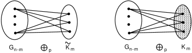
Figure 11: The $SO(m)$-invariant graphs of order $n$. The partial join $\oplus_{p}$ has $p=2$ in these examples.

The $SO(m)$-invariant graphs have a graph-local discrete symmetry $S_{m}$ which permutes the labels of the points of $\tilde{{\cal K}}_{m}$ or ${\cal K}_{m}$, and, conversely, any graph with a graph-local symmetry $S_{m}$ is an $SO(m)$-invariant graph. A prescription to construct the general $h(SO(n)_{diag})$-invariant graph is given in Ref. [93].

Some further properties of Lie $h$-invariant graphs are as follows.
A. Symmetry hierarchy in graph theory. The graph hierarchy,

$${\rm graphs}\supset\supset\mbox{graphs with symmetry}\phantom{WWWWWWWWWWW}$$

$$\supset\supset\;\mbox{Lie}\;h\mbox{-invariant graphs}\phantom{W}$$

$$\phantom{WWWWWWWWWWWW}\supset\supset\;\mbox{affine-Sugawara nested graphs}$$ (8.1.18)

is a special case of the symmetry hierarchy (6.1.4) in ICFT. In this hierarchy, the graphs with any symmetry classify the $H$-invariant CFTs of $SO(n)_{diag}$. The Lie $h$-invariant graphs, which classify the Lie $h$-invariant CFTs of $SO(n)_{diag}$, are those with the special graph-local symmetry described above. The affine-Sugawara nested graphs classify the affine-Sugawara nests in $SO(n)_{diag}$, which are the conventional RCFTs of the ansatz. It follows that the generic Lie $h$-invariant level-family is a set of new (generically unitary and irrational) CFTs.

B. Graphical identification of (1,0) and (0,0) operators. The Lie $h$-invariant graphs also tell us how the Lie $h$ symmetry is realized in the Lie $h$-invariant CFTs. In particular, it has been shown [93] that the $h=SO(m)$ currents $J_{ij}=J_{\mu\nu}$ are either (1,0) or (0,0) operators,

$$J_{ij}\;{\rm is}\;{\rm a}\;(1,0)\;{\rm operator}\;{\rm of}\;L({\cal G}_{n-m}\oplus_{p}{\cal K}_{m})\;{\rm when}\;i,j\in{\cal K}_{m}$$ (8.1.19a)

$$J_{ij}\;{\rm is}\;{\rm a}\;(0,0)\;{\rm operator}\;{\rm of}\;L({\cal G}_{n-m}\oplus_{p}{\tilde{\cal K}}_{m})\;{\rm when}\;i,j\in{\tilde{\cal K}}_{m}$$ (8.1.19b)

that is, the edges or missing edges in ${\cal K}_{m}$ or $\tilde{{\cal K}}_{m}$ correspond to (1,0) or (0,0) currents respectively. It follows that the Lie subgroup symmetry is realized globally for the theories with a ${\cal K}_{m}$ component and locally for the theories with a $\tilde{{\cal K}}_{m}$ component. (The $g/h$ coset constructions are examples of the latter case.) Similarly, each subgroup $SO(m_{i})$ in the general case $h(SO(n)_{diag})=\times_{i=1}^{N}SO(m_{i})$ is realized either locally or globally [93].

C. Generalized complementarity in graph theory. Generalized K-conjugation in ICFT (and in particular K_g/h-conjugation) was reviewed in Section 2.2. The generalized K-conjugations are realized in graph theory as new generalized complementarities in the space of Lie $h$-invariant graphs. In particular, K_g/h-conjugation corresponds to a new K_g/h-complementarity through the coset graphs (8.1.6), which is defined on the subspace of graphs with a local Lie $h$ symmetry.

Moreover, the self K_g/h-conjugate level-families of $SO(n)_{diag}$ live with $c=c_{g/h}/2$ on the self K_g/h-complementary graphs, for which the graph and its K_g/h-complement are isomorphic. Examples of these graphs are given in [93], which also gives the exact form of the self K_SO(6)/SO(2)-conjugate level-families (6.3.4). Although these graphs have been counted on small manifolds [93], enumeration of the self K_g/h-complementary graphs is an open problem in graph theory.

Many other generalized K-conjugations exist [93], which correspond to generalized complementarities through the affine-Sugawara nested graphs. In parallel with the self K_g/h-complementary graphs, it would be interesting to find examples of self-complementary graphs for all the generalized complementarities.

D. The development above describes only the Lie $h$-invariant graphs of conventional graph theory, which live on $SO(n)$. It would be interesting to combine the general theory of Lie $h$-invariant CFTs (see Section 6.1.1) and generalized graph theory on Lie $g$ to characterize the Lie $h$-invariant graphs on other manifolds.

8.2 Conventional Graph Theory in the SME

8.2.1 Graph theory of superconformal level-families

The superconformal ansatz $SO(n)_{diag}[N=1]$ is a consistent ansatz of the SME on $SO(n)_{x}\times SO({\rm dim}\,SO(n))_{\tau_{n}}$ with supercurrent [73]

$$G(z)=\sum_{i<j}\Lambda_{ij}J_{ij}(z)S_{ij}(z)-i\sqrt{\tau_{n}\psi_{n}^{2}\over 2}\sum_{i<j<l}t(ijl)\hbox{ }^{o}_{o}S_{ij}(z)S_{il}(z)S_{jl}(z)\hbox{ }^{o}_{o}$$ (8.2.1a)

$$e^{ij,kl}=\Lambda_{ij}\delta_{ik}\delta_{jl}\quad,\quad t^{ij,il,jl}=t(ijl)f^{ij,il,jl}$$ (8.2.1b)

where $\Lambda_{ij}$ and $t(ijl)$ are the vielbein and the three-form variables of the ansatz, and $\tau_{n}$ is defined in (8.1.2b). The ansatz contains at least two large classes of superconformal field theories, which are seen respectively in the vielbein-dominated and the three-form-dominated high-level expansions (7.2.16b).

In the case of the vielbein-dominated expansion, one finds a (signed) graph-theoretic classification in which the high-level vielbein $\Lambda_{ij}^{(0)}$ defines the edges $ij$ of the graphs ${\cal G}$ and the high-level three-form $t(ijl)^{(0)}$ lives on the unordered triplets $ijl$ of the graphs. The roles of $\Lambda$ and $t$ are reversed in the three-form-dominated expansion, with the vielbein living on the 1-boundaries of a set of 2-complexes ${\cal C}$ defined by the 3-forms. In both cases, the set of superconformal field theories is much larger than a graph theory unit because the variables which live on the geometric structures can assume many values.

Within this ansatz, detailed studies have been made of the following two consistent subansätze [99, 100],

$$SO(n)_{diag}[\scriptstyle{N=1\atop t=0}\displaystyle]\;\;:\;\;\;t(ijl)=0\quad,\quad\mbox{no graph triangles in}\;\,{\cal G}$$ (8.2.2a)

$$SO({\rm dim}\,SO(n))[N=1]\;\;:\Lambda_{ij}=0\quad,\quad\mbox{no simplex-triplets in}\;\,{\cal C}$$ (8.2.2b)

which live in the vielbein- and three-form-dominated expansions respectively. The first subansatz (8.2.2a) is the superconformal metric ansatz $SO(n)_{diag}[\scriptstyle{N=1\atop t=0}\displaystyle]\subset g_{metric}[\scriptstyle{N=1\atop t=0}\displaystyle]$ (see Section 7.4.2), which, as discussed below, is classified by the triangle-free conventional graphs. The purely fermionic ansatz (8.2.2b) is classified by the triplet-free two-dimensional simplicial complexes, where a simplex-triplet is three mutually-adjacent 2-simplices.

Both of these subansätze reduce the SME to a set of linear equations (see also Section 7.4.2), whose solutions are generically-new superconformal field theories with rational central charge. In both cases, moreover, one finds many candidates for new RCFTs. In what follows we discuss the constructions on triangle-free graphs in further detail, referring the reader to [100] for a discussion of the constructions on the 2-complexes.

8.2.2 Superconformal constructions on triangle-free graphs

We discuss the superconformal metric ansatz $SO(n)_{diag}[\scriptstyle{N=1\atop t=0}\displaystyle]$ (see Ref. [99] and eq.(7.4.18a)), whose automorphically-inequivalent level-families live on each triangle-free conventional graph ${\cal G}_{n}$ of order $n$,

$$\forall i,j,k:\ \ \theta_{ij}({\cal G}_{n})\theta_{jk}({\cal G}_{n})\theta_{ki}({\cal G}_{n})=0\quad.$$ (8.2.3)

The edge-variables $\lambda_{ij}({\cal G}_{n},x)=k\Lambda_{ij}^{2}({\cal G}_{n},x)$ of the level-families live on the edges $(ij)$ of each triangle-free graph. The supercurrent of the ansatz is a special case of eq.(7.4.22a),

$$G({\cal G}_{n},x)=\sum_{(ij)\in E({\cal G})}\sqrt{{\lambda_{ij}({\cal G}_{n},x)\over k}}J_{ij}S_{ij}$$ (8.2.4)

and unitarity on $x\in{\rm I\!N}$ requires $\lambda_{ij}\geq 0$.

The linear equations of the ansatz

$$\sum_{k<l}({{\mathchoice{\rm 1\mskip-4.0mul}{\rm 1\mskip-4.0mul}{\rm 1\mskip-4.5mul}{\rm 1\mskip-5.0mul}}}+\frac{\tau_{n}}{x}A^{(1,1)}({\cal G}_{n}))_{ij,kl}\lambda_{kl}({\cal G}_{n},x)=1$$ (8.2.5a)

$$c({\cal G}_{n},x)=\frac{3}{2}\sum_{i<j}\lambda_{ij}({\cal G}_{n},x)$$ (8.2.5b)

are a special case of eq.(7.4.23c). Here, ${\mathchoice{\rm 1\mskip-4.0mul}{\rm 1\mskip-4.0mul}{\rm 1\mskip-4.5mul}{\rm 1\mskip-5.0mul}}$ is the unit matrix in the space of graph edges of ${\cal G}_{n}$ and $A^{(1,1)}_{ij,kl}({\cal G}_{n})$ is the edge-adjacency matrix (7.3.38) of ${\cal G}_{n}$. The linear system (8.2.5b) shows nearest-neighbor coupling of the edge-variables on the generalized lattice defined by each conventional graph.

The level-families of $SO(n)_{diag}[{{N=1}\atop{t=0}}]$ are generically unitary with rational central charge, but the generic level-family is a new set of superconformal field theories because:
1. the generic stress tensor has irrational coefficients, so that irrational conformal weights occur in the generic construction,
2. the conventional N=1 constructions in the subansatz are a small subset of the level-families on triangle-free graphs,
3. the central charge of the generic construction cannot be expressed as sums and differences of affine-Sugawara central charges.
In these broad features, the level-families on triangle-free graphs parallel the self K-conjugate constructions [97, 98], which have half affine-Sugawara central charge and generically irrational conformal weights.

Table 2: The triangle-free graphs of $SO(6)_{diag}[{N=1\atop t=0}]$.

To understand item 3 above, see Table 2, which shows the central charges of the level-families of $SO(6)_{diag}[{{N=1}\atop{t=0}}]$ on the triangle-free graphs of order 6. In this table, all constructions are unitary on level $x\in{\rm I\!N}$ unless indicated explicitly (e.g., $x\neq 1$) with the central charge. Conventional superconformal constructions are labelled by $h$ (subgroup construction) and KS (Kazama-Suzuki coset construction [126]), while new superconformal level-families are marked with the usual #.

Consider, for example, the first new level-family of the table, which is the path graph of order 4. The denominator of this central charge has roots at irrational level $x=\pm\sqrt{2}$, so the level-family cannot be obtained by coset construction. (Sums and differences of affine-Sugawara central charges can diverge only at rational levels.) Similarly, the generic level family $\lambda_{ij}({\cal G}_{n},x)$ is new because the roots of the denominator of $c({\cal G}_{n},x)$ are among the generically-irrational eigenvalues of the edge-adjacency matrix (7.3.38) of its graph ${\cal G}_{n}$.

Candidates for new RCFTs

Because of the square roots in the stress tensor, it is expected that the generic level-family in $SO(n)_{diag}[{{N=1}\atop{t=0}}]$ has irrational conformal weights. On the other hand, there are many level-families which appear to be new RCFTs (beyond $h$ and $g/h$) because the square roots cancel. These constructions live among the level-families (7.4.25b) on the edge-regular triangle-free graphs, which have

$$\lambda({\cal G})={x\over x+\tau_{n}D({\cal G})}\quad,\quad c({\cal G})=\frac{3x{\rm dim}\,E({\cal G})}{2(x+\tau_{n}D({\cal G}))}$$ (8.2.6)

where $D({\cal G})$ is the edge-degree of the graph. In this case, the stress tensor has rational coefficients on $x\in{\rm I\!N}$ because $\sqrt{\lambda_{rs}\lambda_{kl}}=\lambda$. The conventional superconformal level-families of the subansatz are a small subset of the level-families on edge-regular graphs, but many candidates for new RCFTs are also included (e.g. the cycles $C_{5}$ and $C_{6}$ in Table 2). Low-lying conformal weights in these theories are rational, but it is an open question whether these theories are truly new RCFTs, with entirely rational conformal weights.

We finally mention that graph spectral theory [163] has been used [99] to identify superconformal quadratic deformations at particular levels on almost all edge-regular triangle-free graphs.

8.3 Bosonic N=2 Superconformal Constructions

Kazama and Suzuki [124] and Cohen and Gepner [34] have found a graph theory unit of N=2 superconformal constructions in the interacting bosonic models (IBMs). It is suspected by the authors that this set of IBMs live in the N=2 SME (see Section 4.2), but this has not yet been shown.

In this construction, the ansatz for the supercurrents is [124],

$$G_{+}(z)=\sum_{i=1}^{n}g(\gamma^{(i)}){\rm e}^{i\gamma^{(i)}\cdot\phi(z)}\quad,\quad G_{-}(z)=\sum_{i=1}^{n}g(\gamma^{(i)})^{\dagger}{\rm e}^{-i\gamma^{(i)}\cdot\phi(z)}$$ (8.3.1a)

$$\gamma^{(i)}\cdot\gamma^{(j)}=\left\{\matrix{3&i=j\cr 0\;\,\mbox{or}\;\,1&i\neq j\cr}\right.$$ (8.3.1b)

where $\phi_{A}$ and $\gamma^{(i)}_{A}$, $A=1\ldots D$ are respectively a set of bosons and any set of vectors which satisfy (8.3.1b). N=2 superconformal symmetry is obtained when [124],

$$\sum_{j=1}^{n}\Gamma_{ij}x_{j}=2\quad,\quad x_{i}\equiv|g(\gamma^{(i)})|^{2}$$ (8.3.2a)

$$c=\frac{3}{2}\sum_{i=1}^{n}x_{i}$$ (8.3.2b)

where $\Gamma_{ij}\equiv\gamma^{(i)}\cdot\gamma^{(j)}$. Note that the off-diagonal part of $\Gamma_{ij}$ can be viewed as the adjacency-matrix $\theta_{ij}$ of a graph of order $n$, so this system is also a graph theory unit of superconformal constructions [34].

In particular, the central charge [124],

$$c={3n\over 3+d}\geq 3$$ (8.3.3)

is obtained on the regular graphs of order $n$ with degree $d$. It was argued in [34] that there are an infinite number of CFTs at each value (8.3.3) of the central charge, and, among these, there are an infinite number of new RCFTs, with entirely rational conformal weights.

Ref. [34] also discusses a method for obtaining the finite-level fusion rules of new CFTs (see Section 11 for the high-level fusion rules of ICFT).

Part III The Dynamics of ICFT

9 Dynamics on the Sphere

We turn now to the operator formulation of the dynamics of ICFT, including the Ward identities satisfied by the natural correlators and characters of ICFT on the sphere and the torus. Because the stress tensors come in commuting K-conjugate pairs, the central notions here include biconformal field theory and factorization of the bicorrelators and bicharacters to obtain the correlators and characters of the individual CFTs.

Biconformal fields were first obtained for the coset constructions by Halpern in Ref.  [86]. Generalization of the biconformal fields to all ICFT was given by Halpern and Obers in Ref.  [103], where these fields were used to derive the affine-Virasoro Ward identities for the bicorrelators on the sphere. Factorization and solutions of the Ward identities were discussed in Ref.  [104], including the general solution which shows a universal braiding for all ICFT. The flat-connection form of the Ward identities was obtained in Ref.  [105]. In this form, one sees that the Ward identities of ICFT are generalized Knizhnik-Zamolodchikov equations, which include the conventional Knizhnik-Zamolodchikov equation [129] as a special case. The parallel development on the torus is reviewed in Section 13.

Short reviews of these developments are found in Refs. [88] and [89].

9.1 Background: Biconformal Field Theory

We recall from Part I that the general affine-Virasoro construction gives two commuting conformal stress tensors $T$ and $\tilde{T}$, called a K-conjugate pair [18, 91],

$$T=L^{ab}\hbox{ }^{*}_{*}J_{a}J_{b}\hbox{ }^{*}_{*}=\sum_{m}L(m)z^{-m-2}$$ (9.1.1a)

$$\tilde{T}=\tilde{L}^{ab}\hbox{ }^{*}_{*}J_{a}J_{b}\hbox{ }^{*}_{*}=\sum_{m}\tilde{L}(m)z^{-m-2}$$ (9.1.1b)

$$T_{g}=T+\tilde{T}=L_{g}^{ab}\hbox{ }^{*}_{*}J_{a}J_{b}\hbox{ }^{*}_{*}=\sum_{m}L_{g}(m)z^{-m-2}$$ (9.1.1c)

$$[L(m),\tilde{L}(n)]=0$$ (9.1.1d)

where each pair sums to the affine-Sugawara construction $T_{g}$. It is clear that, as constructed on the affine Hilbert space, the natural structure of ICFT is a large set of biconformal field theories [86, 103], where each biconformal field theory has two commuting stress tensors.

The decomposition $T_{g}=T+\tilde{T}$ strongly suggests that, for each K-conjugate pair, the affine-Sugawara construction is a tensor product CFT, formed by tensoring the conformal field theories of $T$ and $\tilde{T}$. In practice, one faces the inverse problem, namely the definition of the $T$ theory by modding out the $\tilde{T}$ theory and vice versa. In the operator approach to the dynamics of ICFT [103, 104, 105], the biconformal structure is central and one uses null states of the Knizhnik-Zamolodchikov (KZ) type [129] to derive Ward identities for the biconformal correlators [103]. Then one must learn to factorize [103, 104] the biconformal correlators into the conformal correlators of $T$ and $\tilde{T}$.

This discussion cannot be complete without mention of the chiral null-state approach [23, 43, 44], to which we owe a deep understanding of conventional RCFT. In this approach, one uses null states in modules of extended Virasoro algebras [147, 156, 183, 55, 54] to bypass the biconformal structure $T_{g}=T_{h}+T_{g/h}$ of $h$ and the $g/h$ coset constructions, obtaining directly the BPZ equations for the coset correlators. Although beautifully crafted for the coset constructions, this technique apparently has little to say about the affine-Sugawara constructions and the general ICFT, for which one is led to consider the more general (biconformal) dynamics of the KZ type. Moreover, the approach through biconformal field theory gives an alternate description of the coset constructions, which has led to new results for the coset constructions on the sphere and the torus (see Sections 10 and 13.7).

9.2 Biprimary States

Given a biconformal field theory, it is natural to decompose the affine Hilbert space into Virasoro biprimary and bisecondary states [86, 103], where Virasoro biprimary states $|\Delta,\tilde{\Delta}\rangle$ are Virasoro primary under both commuting K-conjugate Virasoro operators,

$$L(m)|\Delta,\tilde{\Delta}\rangle=\delta_{m,0}\Delta|\Delta,\tilde{\Delta}\rangle\quad,\quad m\geq 0$$ (9.2.1a)

$$\tilde{L}(m)|\Delta,\tilde{\Delta}\rangle=\delta_{m,0}\tilde{\Delta}|\Delta,\tilde{\Delta}\rangle\quad,\quad m\geq 0$$ (9.2.1b)

$$\Delta+\tilde{\Delta}=\Delta_{g}.$$ (9.2.1c)

In (9.2.1c), $\Delta,\tilde{\Delta},$ and $\Delta_{g}$ are the conformal weights under $T,\tilde{T},$ and $T_{g}$ respectively. Virasoro bisecondary states are then formed as usual, by applying the negative modes of $T$ and $\tilde{T}$ to the biprimary states.

A useful characterization of biprimary states is as follows.

Proposition. Necessary and sufficient conditions for a state $|\phi\rangle$ to be Virasoro biprimary are

$$L_{g}(m)|\phi\rangle=\delta_{m,0}\Delta_{g}|\phi\rangle\quad,\quad m\geq 0$$ (9.2.2a)

$$L(0)|\phi\rangle=\Delta|\phi\rangle$$ (9.2.2b)

where any state which satisfies the condition (9.2.2a) is called an affine-Sugawara primary state.
Proof. According to (9.2.1c) and $T_{g}=T+\tilde{T}$, the conditions (9.2.2b) are necessary. To prove sufficiency, one checks that $|\phi\rangle$ is Virasoro primary under $T$,

$$L(m)|\phi\rangle={1\over m}[L(m),L(0)]|\phi\rangle={1\over m}[L_{g}(m),L(0)]|\phi\rangle=0\quad,\quad m>0$$ (9.2.3)

using the Virasoro algebra of $T$, $T_{g}=T+\tilde{T}$ and $[L(m),\tilde{L}(n)]=0$. Using $T_{g}=T+\tilde{T}$ once more, one easily checks that $|\phi\rangle$ is also Virasoro primary under $\tilde{T}$. $\Box$

An explicit construction of all biprimary states has not yet been found, but many examples are known. The canonical examples are the affine primary states $|\phi\rangle=|R_{\cal T}\rangle^{\alpha},\alpha=1\ldots\dim{\cal T}$, which transform in matrix irrep ${\cal T}$ of $g$. In an $L$- basis of ${\cal T}$ [86, 94, 103], these biprimary states are called the $L^{ab}$-broken affine primary states, which also satisfy

$$J_{a}(m)|R_{\cal T}\rangle^{\alpha}=\delta_{m,0}|R_{\cal T}\rangle^{\beta}({\cal T}_{a})_{\beta}{}^{\alpha}\quad,\quad m\geq 0$$ (9.2.4a)

$$\tilde{L}^{ab}({\cal T}_{a}{\cal T}_{b})_{\alpha}{}^{\beta}=\tilde{\Delta}_{\alpha}({\cal T})\delta_{\alpha}{}^{\beta}\quad,\quad L^{ab}({\cal T}_{a}{\cal T}_{b})_{\alpha}{}^{\beta}=\Delta_{\alpha}({\cal T})\delta_{\alpha}{}^{\beta}$$ (9.2.4b)

$$\tilde{L}(0)|R_{\cal T}\rangle^{\alpha}=\tilde{\Delta}_{\alpha}({\cal T})|R_{\cal T}\rangle^{\alpha}\quad,\quad L(0)|R_{\cal T}\rangle^{\alpha}=\Delta_{\alpha}({\cal T})|R_{\cal T}\rangle^{\alpha}$$ (9.2.4c)

$$\tilde{\Delta}_{\alpha}({\cal T})+\Delta_{\alpha}({\cal T})=\Delta_{g}({\cal T})$$ (9.2.4d)

where $\Delta_{g}({\cal T})$ is the $\alpha$-independent conformal weight under $T_{g}$ and $\tilde{\Delta}_{\alpha}({\cal T})$ and $\Delta_{\alpha}({\cal T})$ are the $L^{ab}$-broken conformal weights under $\tilde{T}$ and $T$ respectively. More generally, $L$-bases are the eigenbases of the conformal weight matrices, such as (9.2.4b), which occur at each level of the affine irrep. Other examples of biprimary states include the one-current states $J_{A}(-1)|0\rangle,A=1\ldots\dim g$, whose conformal weights satisfy $\tilde{\Delta}_{A}+\Delta_{A}=\Delta_{g}=1$.

9.3 Biprimary Fields

In biconformal field theory, the natural generalization of Virasoro primary fields are the Virasoro biprimary fields, which are simultaneously Virasoro primary under both commuting stress tensors $\tilde{T}$ and $T$. These fields were first constructed for $h$ and the $g/h$ coset constructions in Ref.  [86], where they were called bitensor fields. Generalization to all ICFT was given in Ref.  [103].

To construct the biprimary fields, one begins with an affine-Sugawara primary field $\phi_{g}$, which satisfies

$$T_{g}(z)\phi_{g}(w)=\left({\Delta_{g}\over(z-w)^{2}}+{\partial_{w}\over z-w}\right)\phi_{g}(w)+{\rm reg.}$$ (9.3.1a)

$$\phi_{g}(0)|0\rangle=|\phi\rangle$$ (9.3.1b)

where an $L$-basis for $\phi_{g}$ is assumed so that $|\phi\rangle$ is Virasoro biprimary under $\tilde{T}$ and $T$. Examples of affine-Sugawara primary fields include the affine primary fields and the currents,

$$T_{g}(z)R_{g}^{\alpha}({\cal T},w)=\left({\Delta_{g}({\cal T})\over(z-w)^{2}}+{\partial_{w}\over z-w}\right)R_{g}^{\alpha}(w)+{\rm reg.}$$ (9.3.2a)

$$T_{g}(z)J_{A}(w)=\left({1\over(z-w)^{2}}+{\partial_{w}\over z-w}\right)J_{A}(w)+{\rm reg.}$$ (9.3.2b)

in their respective $L$-bases. It should be noted that, although (9.3.2a) is usually assumed [129] for the affine primary fields, the form is strictly correct only for integer levels of affine compact $g$. This subtlety is discussed in Ref.  [103], which finds an extra zero-norm operator contribution for non-unitary affine-Sugawara constructions.

Although they create biprimary states, the affine-Sugawara primary fields are not Virasoro primary under $\tilde{T}$ and $T$. Instead, they satisfy the relations [158],

$$\tilde{T}(z)\phi_{g}(w)={\tilde{\Delta}\phi_{g}(w)\over(z-w)^{2}}+{\partial_{w}\phi_{g}(w)+\tilde{\delta}\phi_{g}(w)\over z-w}+{\rm reg.}$$ (9.3.3a)

$$T(z)\phi_{g}(w)={\Delta\phi_{g}(w)\over(z-w)^{2}}+{\partial_{w}\phi_{g}(w)+\delta\phi_{g}(w)\over z-w}+{\rm reg.}$$ (9.3.3b)

where $\tilde{\Delta}$ and $\Delta$ are the conformal weights of $|\phi\rangle$ under $\tilde{T}$ and $T$. The extra terms $\tilde{\delta}\phi_{g}$ and $\delta\phi_{g}$ in (9.3.3b),

$$\tilde{\delta}\phi_{g}=-[L(-1),\phi_{g}]\quad,\quad\delta\phi_{g}=-[\tilde{L}(-1),\phi_{g}]$$ (9.3.4)

are generated by the existence of the non-trivial K-conjugate theories.

We turn now to the Virasoro biprimary fields $\phi({\tilde{z}},z)$, whose job it is to compensate for these extra terms. In particular, the biprimary fields are Virasoro primary under both $\tilde{T}$ and $T$,

$$\tilde{T}({\tilde{z}})\phi({\tilde{w}},w)=\left({\tilde{\Delta}\over({\tilde{z}}-{\tilde{w}})^{2}}+{\partial_{\tilde{w}}\over{\tilde{z}}-{\tilde{w}}}\right)\phi({\tilde{w}},w)+\mbox{reg. in $({\tilde{z}}-{\tilde{w}})$}$$ (9.3.5a)

$$T(z)\phi({\tilde{w}},w)=\left({\Delta\over(z-w)^{2}}+{\partial_{w}\over z-w}\right)\phi({\tilde{w}},w)+\mbox{reg. in $(z-w)$}$$ (9.3.5b)

$$\phi(0,0)|0\rangle=\phi_{g}(0)|0\rangle=|\phi\rangle$$ (9.3.5c)

where $\tilde{T}$ and $T$ operate on ${\tilde{w}}$ and $w$ respectively.

The explicit construction of these bilocal fields is remarkably simple [86, 103], involving only $SL(2,{\rm I\!R})$ boosts of the affine-Sugawara primary fields. Because the biprimary fields are of central interest, we give a number of equivalent forms,

$$\phi({\tilde{z}},z) = z^{L(0)}{\tilde{z}}^{\tilde{L}(0)}\phi_{g}(1)z^{-L(0)-\Delta}{\tilde{z}}^{-\tilde{L}(0)-\tilde{\Delta}}$$ (9.3.6a)

$$= \left({{\tilde{z}}\over z}\right)^{\tilde{L}(0)}\phi_{g}(z)\left(z\over{\tilde{z}}\right)^{\tilde{L}(0)+\tilde{\Delta}}$$ (9.3.6b)

$$= \left({z\over{\tilde{z}}}\right)^{L(0)}\phi_{g}({\tilde{z}})\left({\tilde{z}}\over z\right)^{L(0)+\Delta}$$ (9.3.6c)

$$= e^{({\tilde{z}}-z)\tilde{L}(-1)}\phi_{g}(z)e^{(z-{\tilde{z}})\tilde{L}(-1)}$$ (9.3.6d)

$$= e^{(z-{\tilde{z}})L(-1)}\phi_{g}({\tilde{z}})e^{({\tilde{z}}-z)L(-1)}.$$ (9.3.6e)

The first line (9.3.6a) is the original form of the biprimary fields [86], and the alternate forms of (9.3d,e),

$$\phi({\tilde{z}},z) = \exp\left[({\tilde{z}}-z)\oint_{z}{dw\over 2\pi i}\tilde{T}(w)\right]\phi_{g}(z)$$ (9.3.7)

$$= \exp\left[(z-{\tilde{z}})\oint_{\tilde{z}}{dw\over 2\pi i}T(w)\right]\phi_{g}({\tilde{z}})$$

have also been employed [105].

Other useful properties of the biprimary fields include

$$\langle\phi({\tilde{z}},z)\rangle=0$$ (9.3.8a)

$$\phi(z,z)=\phi_{g}(z)$$ (9.3.8b)

where the average (9.3.8a) is in the affine vacuum $|0\rangle$ and (9.3.8b) says that, on the affine-Sugawara line ${\tilde{z}}=z$, the biprimary fields are equal to the affine-Sugawara primary fields.

Examples of biprimary fields include the biprimary fields of the $L^{ab}$-broken affine primary fields and the $L^{ab}$-broken currents

$$R^{\alpha}({\cal T},{\tilde{z}},z)=\exp\left[({\tilde{z}}-z)\oint_{z}{dw\over 2\pi i}\tilde{T}(w)\right]R_{g}^{\alpha}({\cal T},z)$$ (9.3.9a)

$$\tilde{\Delta}_{\alpha}({\cal T})+\Delta_{\alpha}({\cal T})=\Delta_{g}({\cal T})$$ (9.3.9b)

$${\cal J}_{A}({\tilde{z}},z)=\exp\left[({\tilde{z}}-z)\oint_{z}{dw\over 2\pi i}\tilde{T}(w)\right]J_{A}(z)$$ (9.3.9c)

$$\tilde{\Delta}_{A}+\Delta_{A}=1$$ (9.3.9d)

where $\alpha=1\ldots\dim{\cal T}$ and $A=1\ldots\dim g$.

9.4 Bicorrelators

Biconformal correlators, or bicorrelators, are averages of biconformal fields in the affine vacuum. For the biprimary fields, one has the $n$-point bicorrelators,

$$\Phi({\tilde{z}},z)\equiv\langle\phi_{1}({\tilde{z}}_{1},z_{1})\cdots\phi_{n}({\tilde{z}}_{n},z_{n})\rangle$$ (9.4.1a)

$$\Phi(z,z)=\Phi_{g}(z)=\langle\phi_{g,1}(z_{1})\cdots\phi_{g,n}(z_{n})\rangle$$ (9.4.1b)

which reduce, on the affine-Sugawara line ${\tilde{z}}=z$, to the affine-Sugawara correlators of the affine-Sugawara primary fields. In general, the affine-Sugawara correlators also satisfy a $g$-global Ward identity. For example, one has

$$A^{\alpha}({\tilde{z}},z)=\langle R^{\alpha_{1}}({\cal T}^{1},{\tilde{z}}_{1},z_{1})\cdots R^{\alpha_{n}}({\cal T}^{n},{\tilde{z}}_{n},z_{n})\rangle$$ (9.4.2a)

$$A^{\alpha}(z,z)=A_{g}^{\alpha}(z)=\langle R^{\alpha_{1}}_{g}({\cal T}^{1},z_{1})\cdots R^{\alpha_{n}}_{g}({\cal T}^{n},z_{n})\rangle$$ (9.4.2b)

$$A_{g}^{\beta}(z)\left(\sum_{i=1}^{n}{\cal T}_{a}^{i}\right)_{\beta}^{~{}\alpha}=0\quad,\quad a=1\ldots\dim g$$ (9.4.2c)

when broken affine primary fields $\phi^{\alpha}=R^{\alpha}$ are chosen for the bicorrelator.

The two- and three-point functions and leading term OPE’s of biprimary fields can be determined [103] from $SL(2,{\rm I\!R})\times SL(2,{\rm I\!R})$ covariance and knowledge of the corresponding quantities for the affine-Sugawara primary fields.

As examples, we give the results for three broken affine primary fields,

$$\langle R^{\alpha_{1}}({\cal T}^{1},{\tilde{z}}_{1},z_{1})R^{\alpha_{2}}({\cal T}^{2},{\tilde{z}}_{2},z_{2})R^{\alpha_{3}}({\cal T}^{3},{\tilde{z}}_{3},z_{3})\rangle={Y_{g}^{\alpha_{1}\alpha_{2}\alpha_{3}}\over{\tilde{z}}_{12}^{\tilde{\gamma}_{12}}{\tilde{z}}_{13}^{\tilde{\gamma}_{13}}{\tilde{z}}_{23}^{\tilde{\gamma}_{23}}z_{12}^{\gamma_{12}}z_{13}^{\gamma_{13}}z_{23}^{\gamma_{23}}}$$ (9.4.3a)

$$R^{\alpha_{1}}({\cal T}^{1},{\tilde{z}}_{1},z_{1})R^{\alpha_{2}}({\cal T}^{2},{\tilde{z}}_{2},z_{2})\smash{\mathop{\sim}\limits_{{\tilde{z}}_{12},z_{12}\rightarrow 0}}\sum_{k,\beta_{k}}{Y_{g}^{\alpha_{1}\alpha_{2}\alpha_{k}}\eta_{\alpha_{k}\beta_{k}}({\cal T}^{k})R^{\beta_{k}}({\cal T}^{k},{\tilde{z}}_{2},z_{2})\over{\tilde{z}}_{12}^{\tilde{\Delta}_{12k}}z_{12}^{\Delta_{12k}}}\;.$$ (9.4.3b)

Here, ${\tilde{z}}_{ij}={\tilde{z}}_{i}-{\tilde{z}}_{j},z_{ij}=z_{i}-z_{j}$, $\eta_{\alpha\beta}({\cal T})$ is the carrier space metric of irrep ${\cal T}$ and

$$\tilde{\gamma}_{ij}=\tilde{\Delta}_{\alpha_{i}}({\cal T}^{i})+\tilde{\Delta}_{\alpha_{j}}({\cal T}^{j})-\tilde{\Delta}_{\alpha_{k}}({\cal T}^{k})$$ (9.4.4a)

$$\gamma_{ij}=\Delta_{\alpha_{i}}({\cal T}^{i})+\Delta_{\alpha_{j}}({\cal T}^{j})-\Delta_{\alpha_{k}}({\cal T}^{k})$$ (9.4.4b)

while $\tilde{\Delta}_{12k}$ and $\Delta_{12k}$ are given by (9.4.4b) with $\alpha_{k}\rightarrow\beta_{k}$. The coefficient $Y_{g}$ is the invariant affine-Sugawara three-point correlator, which satisfies the $g$-global Ward identity $Y_{g}^{\beta}(\sum_{i=1}^{3}{\cal T}_{a}^{i})_{\beta}{}^{\alpha}=0$. It follows that $Y_{g}^{\alpha_{1}\alpha_{2}\alpha_{k}}$ are the Clebsch-Gordon coefficients for ${\cal T}^{1}\oplus{\cal T}^{2}$ into $\bar{\cal T}^{k}$, taken in a simultaneous $L$-basis of the three irreps ${\cal T}$.

We also mention the bilocal current algebra [103],

$${\cal J}_{A}({\tilde{z}},z){\cal J}_{B}({\tilde{w}},w) \sim {\tilde{z}}\rightarrow{\tilde{w}} z\rightarrow w {G_{AB}\over({\tilde{z}}-{\tilde{w}})^{2\tilde{\Delta}_{A}}(z-w)^{2\Delta_{A}}}\hskip 144.54pt$$ (9.4.5)

$$+\sum_{C}{if_{AB}{}^{C}{\cal J}_{C}({\tilde{w}},w)\over({\tilde{z}}-{\tilde{w}})^{\tilde{\Delta}_{A}+\tilde{\Delta}_{B}-\tilde{\Delta}_{C}}(z-w)^{\Delta_{A}+\Delta_{B}-\Delta_{C}}}$$

satisfied by the biprimary fields of the $L^{ab}$-broken currents. Here, $G_{AB}$ and $f_{AB}{}^{C}$ are the generalized Killing metric and structure constants of $g$, both in the $L$-basis of the one-current states.

See Ref.  [103] for further details on two- and three-point bicorrelators.

More generally, one has the $SL(2,{\rm I\!R})\times SL(2,{\rm I\!R})$ decomposition of the bicorrelators

$$\langle\phi_{1}({\tilde{z}}_{1},z_{1})\cdots\phi_{n}({\tilde{z}}_{n},z_{n})\rangle={Y(\tilde{u},u)\over\prod_{i<j}{\tilde{z}}_{ij}^{\tilde{\gamma}_{ij}(\alpha)}z_{ij}^{\gamma_{ij}(\alpha)}}$$ (9.4.6a)

$$\sum_{j\neq i}\tilde{\gamma}_{ij}(\alpha)=2\tilde{\Delta}_{\alpha_{i}}\quad,\quad\sum_{j\neq i}\gamma_{ij}(\alpha)=2\Delta_{\alpha_{i}}$$ (9.4.6b)

$$\tilde{\gamma}_{ij}(\alpha)+\gamma_{ij}(\alpha)=\gamma_{ij}^{g}\quad,\quad\sum_{j\neq i}\gamma_{ij}^{g}=2\Delta_{i}^{g}$$ (9.4.6c)

$$Y(u,u)=Y_{g}(u)$$ (9.4.6d)

where $\{\tilde{u}\}$ and $\{u\}$ are the sets of independent cross-ratios constructed from $\{{\tilde{z}}_{i}\}$ and $\{z_{i}\}$ respectively, and $Y(\tilde{u},u)$ are the invariant bicorrelators. When $\phi^{\alpha}=R^{\alpha}$, the invariant affine-Sugawara correlators $Y_{g}$ also satisfy the $g$-global Ward identity $Y_{g}\sum_{i=1}^{n}{\cal T}_{a}^{i}=0$.

The biconformal OPE’s, such as (9.4.3b) and (9.4.5), also determine the most singular terms of the bicorrelators. As an example, we give the results for the invariant bicorrelators of four broken affine primaries, using the KZ gauge [129]

$$\tilde{u}={{\tilde{z}}_{12}{\tilde{z}}_{34}\over{\tilde{z}}_{14}{\tilde{z}}_{32}}\quad,\quad u={z_{12}z_{34}\over z_{14}z_{32}}$$ (9.4.7a)

$$\tilde{\gamma}_{12}=\tilde{\gamma}_{13}=\gamma_{12}=\gamma_{13}=0$$ (9.4.7b)

for the invariant decomposition (9.4.6d). The result for the four-point bicorrelators is [90],

$$Y(\tilde{u},u)\smash{\mathop{\sim}\limits_{\tilde{u},u\rightarrow 0}}v_{g}^{(4)}u^{C(L_{g})}\left({\tilde{u}\over u}\right)^{A(\tilde{L})}\left({\tilde{u}\over u}\right)^{-B(\tilde{L})}$$ (9.4.8)

where $v_{g}^{(4)}$ is the $g$-invariant tensor

$$v_{g}^{(4)\alpha}\equiv(-1)^{C(L_{g})}\sum_{k}Y_{g}^{\alpha_{1}\alpha_{2}\alpha_{k}}\eta_{\alpha_{k}\beta_{k}}({\cal T}^{k})Y_{g}^{\beta_{k}\alpha_{3}\alpha_{4}}$$ (9.4.9a)

$$v_{g}^{(4)}\sum_{i=1}^{4}{\cal T}_{a}^{i}=0\quad,\quad a=1\ldots\dim g$$ (9.4.9b)

and $A,B,C$ are the matrices

$$A(L)\equiv L^{ab}({\cal T}_{a}^{1}+{\cal T}_{a}^{2})({\cal T}_{b}^{1}+{\cal T}_{b}^{2})$$ (9.4.10a)

$$B(L)\equiv L^{ab}({\cal T}_{a}^{1}{\cal T}_{b}^{1}+{\cal T}_{a}^{2}{\cal T}_{b}^{2})$$ (9.4.10b)

$$C(L)\equiv A(L)-B(L)=2L^{ab}{\cal T}_{a}^{1}{\cal T}_{b}^{2}.$$ (9.4.10c)

In (9.4.10c) and below, the tensor product ${\cal T}_{a}^{i}{\cal T}_{b}^{j}\equiv\rho_{a}({\cal T}^{i})\otimes\rho_{b}({\cal T}^{j})$ is understood when matrix irreps ${\cal T}^{i}$ are in different spaces $i$.

9.5 The Ward Identities of ICFT

To go beyond the simple considerations of the previous section, one needs the affine-Virasoro Ward identities [103], which provide the central dynamics of ICFT.

The form (9.3.7) of the Virasoro biprimary fields indicates that the biconformal correlators (9.4.1b) can be evaluated as power series about the affine-Sugawara line $\phi(z,z)=\phi_{g}(z)$. Indeed, with $\tilde{\partial}_{j}=\partial/\partial{\tilde{z}}_{j}$ and $\partial_{i}=\partial/\partial z_{i}$, one obtains the formula for the moments of the bicorrelators [103],

$$\left.\tilde{\partial}_{j_{1}}\cdots\tilde{\partial}_{j_{q}}\partial_{i_{1}}\cdots\partial_{i_{p}}\langle\phi_{1}({\tilde{z}}_{1},z_{1})\cdots\phi_{n}({\tilde{z}}_{n},z_{n})\rangle\right|_{{\tilde{z}}=z}\hskip 144.54pt$$

$$= \oint_{{\tilde{z}}_{j_{1}}}{d{\tilde{w}}_{1}\over 2\pi i}\cdots\oint_{{\tilde{z}}_{j_{q}}}{d{\tilde{w}}_{q}\over 2\pi i}\oint_{z_{i_{1}}}{dw_{1}\over 2\pi i}\cdots\oint_{z_{i_{p}}}{dw_{p}\over 2\pi i}\cdot$$ (9.5.1)

$$\quad\cdot\langle\tilde{T}({\tilde{w}}_{1})\cdots\tilde{T}({\tilde{w}}_{q})T(w_{1})\cdots T(w_{p})\phi_{g,1}(z_{1})\cdots\phi_{g,n}(z_{n})\rangle$$

because $\phi(z,z)=\phi_{g}(z)$ and each $\phi({\tilde{z}},z)$ is Virasoro biprimary. The stress tensors on the right of (9.5.1) can be expressed in terms of the currents, and the moments can be evaluated in principle by computation of the averages $\langle$ $\rangle$ in the affine-Sugawara theory on $g$. The relations (9.5.1) are called the Ward identities of ICFT.

We focus here on the simplest case of (9.5.1), that is the Ward identities for the biprimary fields $\phi^{\alpha}({\tilde{z}},z)=R^{\alpha}({\cal T},{\tilde{z}},z)$ of the $L^{ab}$-broken affine primary fields. In this case, the Ward identities take the form [103],

$$\left.\tilde{\partial}_{j_{1}}\cdots\tilde{\partial}_{j_{q}}\partial_{i_{1}}\cdots\partial_{i_{p}}A^{\alpha}\right|_{{\tilde{z}}=z}=A_{g}^{\beta}(W_{j_{1}\cdots j_{q},i_{1}\cdots i_{p}})_{\beta}{}^{\alpha}$$ (9.5.2a)

$$A^{\alpha}({\tilde{z}},z)\equiv\langle R^{\alpha_{1}}({\cal T}^{1},{\tilde{z}}_{1},z_{1})\cdots R^{\alpha_{n}}({\cal T}^{n},{\tilde{z}}_{n},z_{n})\rangle$$ (9.5.2b)

$$A_{g}^{\alpha}(z)=A^{\alpha}(z,z)=\langle R^{\alpha_{1}}_{g}({\cal T}^{1},z_{1})\cdots R^{\alpha_{n}}_{g}({\cal T}^{n},z_{n})\rangle$$ (9.5.2c)

where the coefficients $W_{j_{1}\cdots j_{q}i_{1}\cdots i_{p}}$ are called the affine-Virasoro connection moments. The simple form of (9.5.2a), proportional to the affine-Sugawara correlators $A_{g}$, is due to the simple OPE of the currents with the affine primary fields,

$$J_{a}(z)R_{g}^{\alpha}({\cal T},w)={R_{g}^{\beta}({\cal T},w)\over z-w}({\cal T}_{a})_{\beta}{}^{\alpha}+\mbox{reg.}$$ (9.5.3)

whereas extra inhomogeneous terms are generally obtained for the biprimary fields of broken affine secondaries. See Ref.  [103] for discussion of the corresponding Ward identities associated to the $L^{ab}$-broken currents.

All the connection moments $W_{j_{1}\ldots j_{q},i_{1}\ldots i_{p}}$ may be computed in principle by standard dispersive techniques from the formula [103, 104],

$$A_{g}^{\beta}(z){W_{j_{1}\ldots j_{q},i_{1}\ldots i_{p}}(z)_{\beta}}^{\alpha}=\;\;\;\;\;\;\;\;\;\;\;\;\;\;\;\;\;\;\;\;\;\;\;$$

$$\left[\prod_{r=1}^{q}\tilde{L}^{a_{r}b_{r}}\oint_{z_{j_{r}}}{\mbox{d}\omega_{r}\over 2\pi i}\oint_{\omega_{r}}{\mbox{d}\eta_{r}\over 2\pi i}\;{1\over\eta_{r}-\omega_{r}}\right]\!\left[\prod_{s=1}^{p}L^{c_{s}d_{s}}\oint_{z_{i_{s}}}\!{\mbox{d}\omega_{q+s}\over 2\pi i}\oint_{\omega_{q+s}}\!{\mbox{d}\eta_{q+s}\over 2\pi i}\;{1\over\eta_{q+s}-\omega_{q+s}}\right]$$

$$\times\langle J_{a_{1}}(\eta_{1})J_{b_{1}}(\omega_{1})\ldots J_{a_{q}}(\eta_{q})J_{b_{q}}(\omega_{q})J_{c_{1}}(\eta_{q+1})J_{d_{1}}(\omega_{q+1})\ldots$$

$$\;\;\;\;\;\;\;\;\;\;\;J_{c_{p}}(\eta_{q+p})J_{d_{p}}(\omega_{q+p})R_{g}^{\alpha_{1}}({\cal T}^{1},z_{1})\ldots R_{g}^{\alpha_{n}}({\cal T}^{n},z_{n})\rangle$$ (9.5.4)

since the required averages are in the affine-Sugawara theory on $g$. The computations of the moments increase in complexity with their order $q+p$.

The Ward identities (9.5.2c) prove the existence of the biconformal correlators [103],

$$A^{\alpha}({\tilde{z}},z)=A_{g}^{\beta}(z)\tilde{F}({\tilde{z}},z)_{\beta}{}^{\alpha}=A_{g}^{\beta}({\tilde{z}})F({\tilde{z}},z)_{\beta}{}^{\alpha}$$ (9.5.5a)

$$\tilde{F}({\tilde{z}},z)=\sum_{q=0}^{\infty}{1\over q!}\sum_{j_{1}\ldots j_{q}}({\tilde{z}}_{j_{1}}-z_{j_{1}})\cdots({\tilde{z}}_{j_{q}}-z_{j_{q}})W_{j_{1}\ldots j_{q},0}(z)$$ (9.5.5b)

$$F({\tilde{z}},z)=\sum_{p=0}^{\infty}{1\over p!}\sum_{i_{1}\ldots i_{p}}(z_{i_{1}}-{\tilde{z}}_{i_{1}})\cdots(z_{i_{p}}-{\tilde{z}}_{i_{p}})W_{0,i_{1}\ldots i_{p}}({\tilde{z}})$$ (9.5.5c)

as the indicated Taylor series expansions around the affine-Sugawara line.

9.6 Properties of the Connection Moments

The connection moments have been computed explicitly through order $q+p=2$.

The first-order connection moments are [103],

$$W_{0,i}=2L^{ab}\sum_{j\neq i}^{n}{{\cal T}_{a}^{i}{\cal T}_{b}^{j}\over z_{ij}}\quad,\quad W_{i,0}=2\tilde{L}^{ab}\sum_{j\neq i}^{n}{{\cal T}_{a}^{i}{\cal T}_{b}^{j}\over z_{ij}}$$ (9.6.1)

where ${\cal T}^{i}$ is the matrix irrep of the $i$th broken affine primary field in the bicorrelator. Note that, because of K-conjugation covariance, the sum of the first-order moments is the affine-Sugawara connection $W_{i}^{g}$, which appears in the Knizhnik-Zamolodchikov (KZ) equation [129] for $A_{g}$,

$$W_{i,0}+W_{0,i}=W_{i}^{g}=2L_{g}^{ab}\sum_{j\neq i}^{n}{{\cal T}_{a}^{i}{\cal T}_{b}^{j}\over z_{ij}}$$ (9.6.2a)

$$\partial_{i}A_{g}^{\alpha}=A_{g}^{\beta}(W_{i}^{g})_{\beta}{}^{\alpha}$$ (9.6.2b)

$$A_{g}\sum_{i=1}^{n}{\cal T}_{a}^{i}=0\quad,\quad a=1\ldots\dim g.$$ (9.6.2c)

Indeed, the KZ equation is implied by the sum of the first-order Ward identities,

$$\partial_{i}A_{g}(z)=\left.(\tilde{\partial}_{i}+\partial_{i})A_{g}({\tilde{z}},z)\right|_{{\tilde{z}}=z}=A_{g}(z)W_{i}^{g}(z)$$ (9.6.3)

where the first step in (9.6.3) is a chain rule.

The second-order connection moments are [103],

$$W_{0,ij}=\partial_{i}W_{0,j}+\frac{1}{2}[W_{0,i},W_{0,j}]_{+}+E_{0,ij}\quad,\quad W_{ij,0}=\partial_{i}W_{j,0}+\frac{1}{2}[W_{i,0},W_{j,0}]_{+}+E_{ij,0}$$ (9.6.4a)

$$W_{i,j}=W_{i,0}W_{0,j}+E_{i,j}$$ (9.6.4b)

$$E_{i,j}=-2iL^{da}L^{e(b}{f_{de}}^{c)}\left\{{{\cal T}_{c}^{j}{\cal T}_{b}^{j}{\cal T}_{a}^{i}+{\cal T}_{c}^{i}{\cal T}_{b}^{i}{\cal T}_{a}^{j}\over z_{ij}^{2}}-2\sum_{k\neq i,j}^{n}{{\cal T}_{c}^{k}{\cal T}_{b}^{i}{\cal T}_{a}^{j}\over z_{ij}z_{ik}}\right\}\quad,\quad i\neq j$$ (9.6.4c)

$$E_{0,ij}=-\frac{1}{2}(E_{i,j}+E_{j,i})\quad,\quad E_{ij,0}=E_{0,ij}|_{L\rightarrow\tilde{L}}\quad,\quad E_{i,i}=-\sum_{j\neq i}^{n}E_{i,j}$$ (9.6.4d)

where the Virasoro master equation (2.1.10a) was used to obtain the terms $\partial_{i}W_{0,j}$ and $\partial_{i}W_{j,0}$, which are first order in $L$ and $\tilde{L}$ respectively.

The connection moments have also been computed to all orders for the $g/h$ coset constructions (see Section 10.2), the higher affine-Sugawara nests [104, 105], and the general ICFT at high level on simple $g$ (see Section 11.2). Moreover, the leading singularities as $u\rightarrow 0$ have been obtained for the all-order moments of the general four-point invariant bicorrelators (See Section 9.12).

We turn now to some more general properties of the connection moments.

A. Symmetry. The connection moments $W_{j_{1}\cdots j_{q},i_{1}\cdots i_{p}}$ are symmetric under exchange of any two $j$ labels or any two $i$ labels [103].

B. K-conjugation covariance. The connection moments satisfy [105]

$$W_{j_{1}\cdots j_{q},i_{1}\cdots i_{p}}(\tilde{L},L)=W_{i_{1}\cdots i_{p},j_{1}\cdots j_{q}}(L,\tilde{L})$$ (9.6.5)

under exchange of the K-conjugate theories.

The one-sided connection moments $W_{j_{1}\cdots j_{q},0}(\tilde{L})$ and $W_{0,i_{1}\cdots i_{p}}(L)$ are functions of $\tilde{L}$ and $L$ respectively, and satisfy the K-conjugation covariance [105]

$$W_{j_{1}\cdots j_{q},0}(\tilde{L})=\left.W_{0,j_{1}\cdots j_{q}}(L)\right|_{L=\tilde{L}}$$ (9.6.6a)

$$W_{0,i_{1}\cdots i_{p}}(L)=\left.W_{i_{1}\cdots i_{p},0}(\tilde{L})\right|_{\tilde{L}=L}$$ (9.6.6b)

according to (9.6.5).

C. Consistency relations. The connection moments satisfy the consistency relations

$$(\partial_{i}+W_{i}^{g})W_{j_{1}\cdots j_{q},i_{1}\cdots i_{p}}=W_{j_{1}\cdots j_{q}i,i_{1}\cdots i_{p}}+W_{j_{1}\cdots j_{q},i_{1}\cdots i_{p}i}$$ (9.6.7)

where $W_{00}={\mathchoice{\rm 1\mskip-4.0mul}{\rm 1\mskip-4.0mul}{\rm 1\mskip-4.5mul}{\rm 1\mskip-5.0mul}}$ and $W_{i}^{g}$ is the affine-Sugawara connection in (9.6.2a). These relations were originally derived [103] from simple properties of the biprimary fields, but they are also the integrability conditions for the existence of the biconformal correlators. To understand this, the reader may wish to consider the simple example $f_{qp}=\tilde{\partial}^{q}\partial^{p}f(\tilde{u},u)|_{\tilde{u}=u}$, which satisfies $\partial f_{qp}=f_{q+1,p}+f_{q,p+1}$ for all $f(\tilde{u},u)$.

The consistency relations relate the moments at a fixed order to the moments at one higher order. For example,

$$W_{i}^{g}=W_{i,0}+W_{0,i}$$ (9.6.8a)

$$(\partial_{i}+W_{i}^{g})W_{j,0}=W_{ji,0}+W_{j,i}\quad,\quad(\partial_{i}+W_{i}^{g})W_{0,j}=W_{0,ij}+W_{i,j}$$ (9.6.8b)

are obtained through order $q+p\leq 2$. The first consistency relation (9.6.8a) was encountered in eq.(9.6.2a).

More generally, the consistency relations are deeply connected to the Virasoro master equation. To understand this, note that the moments of order $q+p$ are naively of order $\tilde{L}^{q}L^{p}$, whereas the derivative term in the consistency relations mixes these orders. In particular, the consistency relations (9.6.8b) are satisfied by the explicit forms (9.6.1) and (9.6.4d) of the first- and second-order moments, but only because the master equation, whose form is $L\sim L^{2}$, was used in the results for the second-order moments.

The consistency relations also tell us about a large redundancy in the connection moments. In particular, one may solve the relations to write the general moment in terms of $W_{i}^{g}$ and either of the two sets of one-sided connection moments, for example

$$W_{j_{1}\cdots j_{q},i_{1}\cdots i_{p}}=W_{j_{1}\cdots j_{q},i_{1}\cdots i_{p}}(W_{i}^{g},W_{0,i_{1},\cdots i_{p}}).$$ (9.6.9)

As an illustration, one has from eq.(9.6.8b) that

$$W_{i,0}=W_{i}^{g}-W_{0,i}$$ (9.6.10a)

$$W_{i,j}=(\partial_{i}+W_{i}^{g})W_{0,j}-W_{0,ij}$$ (9.6.10b)

$$W_{ij,0}=(\partial_{i}+W_{i}^{g})(W_{j}^{g}-W_{0,j})-(\partial_{j}+W_{j}^{g})W_{0,i}+W_{0,ij}$$ (9.6.10c)

through order $q+p=2$. The all-order solution of the consistency relations is given in Ref.  [104].

D. Crossing symmetry. The connection moments satisfy the crossing symmetry [104]

$$\qquad\left.W_{j_{1}\cdots j_{q},i_{1}\cdots i_{p}}(z)\right|_{k\leftrightarrow l}=W_{j_{1}\cdots j_{q},i_{1}\cdots i_{p}}(z)\qquad$$ (9.6.11a)

$$k\leftrightarrow l:\qquad{\cal T}^{k}\leftrightarrow{\cal T}^{l}\quad,\quad z_{k}\leftrightarrow z_{l}\quad,\quad\left\{\begin{array}[]{ll}i\rightarrow l&\mbox{when }i=k\\ i\rightarrow k&\mbox{when }i=l\end{array}\right.$$ (9.6.11b)

where $i\in(j_{1}\cdots j_{q},i_{1}\cdots i_{p})$, and $k\leftrightarrow l$ means exchange of ${\cal T}$’s, $z$’s, and indices, as shown in (9.6.11b).

E. $SL(2,{\rm I\!R})\times SL(2,{\rm I\!R})$ covariance. $SL(2,{\rm I\!R})\times SL(2,{\rm I\!R})$ covariance in biconformal field theory was discussed in Section 9.4. For the connection moments, this covariance gives the $L$-relations [105]

$$A_{g}\sum_{i=1}^{n}W_{j_{1}\ldots j_{q},i_{1}\ldots i_{p}i}=0$$ (9.6.12a)

$$A_{g}\left[\sum_{i=1}^{n}z_{i}W_{j_{1}\ldots j_{q},i_{1}\ldots i_{p}i}+(\sum_{i=1}^{n}\Delta_{i}+p)W_{j_{1}\ldots j_{q},i_{1}\ldots i_{p}}\right]=0$$ (9.6.12b)

$$\;\;\;A_{g}\Bigl{[}\sum_{i=1}^{n}z_{i}^{2}W_{j_{1}\ldots j_{q},i_{1}\ldots i_{p}i} + 2(\sum_{i=1}^{n}z_{i}\Delta_{i}+\sum_{\nu=1}^{p}z_{i_{\nu}})W_{j_{1}\ldots j_{q},i_{1}\ldots i_{p}}$$

$$+ 2\sum_{\nu=1}^{p}(\Delta_{i_{\nu}}+\sum_{\mu=\nu+1}^{p}\delta_{i_{\nu},i_{\mu}})W_{j_{1}\ldots j_{q},i_{1}..\hat{i}_{\nu}..i_{p}}\Bigr{]}=0$$

and analogous $\tilde{L}$ relations are obtained from (9.6) with $\Delta\rightarrow\tilde{\Delta}$. In (9.6), the omission of an index is denoted by a hat. It is believed that the $L(0)$ relation in (9.6.12a) is also true without the factor $A_{g}$, but this has not yet been demonstrated beyond order $q+p=2$.

F. Translation sum rule. To state this relation, one first needs the (invertible) evolution operator $A_{g}(z,z_{0})$ of the affine-Sugawara construction on $g$, which satisfies the KZ boundary value problem

$$\partial_{i}A_{g}(z,z_{0})_{\alpha}{}^{\beta}=A_{g}(z,z_{0})_{\alpha}{}^{\gamma}W_{i}^{g}(z)_{\gamma}{}^{\beta}\quad,\quad A_{g}(z_{0},z_{0})_{\alpha}{}^{\beta}=\delta_{\alpha}{}^{\beta}$$ (9.6.13)

where $z_{0}$ is a regular reference point. It follows that

$$A_{g}(z,z_{0})=P^{*}e^{\int_{z_{0}}^{z}dz_{i}^{\prime}W_{i}^{g}(z^{\prime})}$$ (9.6.14a)

$$A_{g}^{-1}(z,z_{0})=A_{g}(z_{0},z)$$ (9.6.14b)

$$A_{g}(z_{3},z_{1})A_{g}(z_{2},z_{3})=A_{g}(z_{2},z_{1})$$ (9.6.14c)

$$A_{g}^{\alpha}(z)=A_{g}^{\beta}(z_{0})A_{g}(z,z_{0})_{\beta}{}^{\alpha}$$ (9.6.14d)

where $P^{*}$ is anti-ordering in $z$ and $A_{g}^{\alpha}(z)$ is the affine-Sugawara correlator in (9.4.2b). Then the translation sum rule [104]

$$\sum_{r,s=0}^{\infty}{1\over r!\,s!}\sum_{l_{1}\ldots l_{r}}^{n}\sum_{k_{1}\ldots k_{s}}^{n}\left[\prod_{\mu=1}^{r}(z_{l_{\mu}}-z^{0}_{l_{\mu}})\right]\left[\,\prod_{\nu=1}^{s}(z_{k_{\nu}}-z^{0}_{k_{\nu}})\right]W_{l_{1}\ldots l_{r}j_{1}\ldots j_{q},k_{1}\ldots k_{s}i_{1}\ldots i_{p}}(z_{0})$$

$$=A_{g}(z,z_{0})W_{j_{1}\ldots j_{q},i_{1}\ldots i_{p}}(z)$$ (9.6.15)

relates the connection moments at different points.

9.7 Knizhnik-Zamolodchikov Null States

The Ward identities (9.5.2c) and the result (9.5.4) for the connection moments were derived by standard OPE methods, using the biprimary fields and current algebra, but many of these identities can also be derived [103] from null states of the Knizhnik-Zamolodchikov (KZ) type, which live in the enveloping algebra of the affine algebra. This is the method used by Knizhnik and Zamolodchikov in the original derivation of the KZ equations [129].

For example, the first KZ null state is

$$|\chi({\cal T})\rangle_{1}^{\alpha}=L(-1)|R_{g}({\cal T})\rangle^{\alpha}-2L^{ab}J_{a}(-1)|R_{g}({\cal T})\rangle^{\beta}({\cal T}_{b})_{\beta}{}^{\alpha}=0$$ (9.7.1)

where $L^{ab}$ is any solution of the Virasoro master equation and $|R_{g}({\cal T})\rangle^{\alpha},\alpha=1\ldots\dim{\cal T}$ is the broken affine primary state corresponding to matrix irrep ${\cal T}$. Using the identities,

$$\langle 0|R_{g}^{\alpha_{1}}({\cal T}^{1},z_{1})\cdots R_{g}^{\alpha_{n}}({\cal T}^{n},z_{n})|\chi({\cal T})\rangle_{1}^{\alpha}=0$$ (9.7.2a)

$$[J_{a}(-1),R_{g}^{\alpha}({\cal T},z)]=z^{-1}R_{g}^{\beta}({\cal T},z)({\cal T}_{a})_{\beta}{}^{\alpha}$$ (9.7.2b)

$$[\tilde{L}(-1),R_{g}^{\alpha}({\cal T},z)]=\left.\tilde{\partial}R^{\alpha}({\cal T},{\tilde{z}},z)\right|_{{\tilde{z}}=z}$$ (9.7.2c)

this null state implies the first-order Ward identity $\partial_{i}A|_{{\tilde{z}}=z}=A_{g}W_{0,i}$ and the form of the first moment $W_{0,i}$. Similarly the Ward identity $\tilde{\partial}_{i}A|_{{\tilde{z}}=z}=A_{g}W_{i,0}$ and the form of $W_{i,0}$ is implied by the K-conjugate null state obtained from (9.7.1) by $L\rightarrow\tilde{L}$. The special case of (9.7.1–2) with $L=L_{g}$ was used by Knizhnik and Zamolodchikov in their derivation of the KZ equations for the affine-Sugawara correlators.

More generally, one may define the $m$th null state of the KZ type as

$$|\chi({\cal T})\rangle_{m}^{\alpha}=|m,L\rangle^{\alpha}-|m,J\rangle^{\alpha}=0\quad,\quad\alpha=1\ldots\dim{\cal T}$$ (9.7.3a)

$$|m,L\rangle^{\alpha}=\left(L(-1)\right)^{m}|R_{g}({\cal T})\rangle^{\alpha}$$ (9.7.3b)

$$L(-1)=2L^{ab}\sum_{n=0}^{\infty}J_{a}(-n-1)J_{b}(n)$$ (9.7.3c)

where $|m,J\rangle^{\alpha}$ is obtained by rewriting $|m,L\rangle^{\alpha}$ in terms of negatively moded currents on $|R_{g}({\cal T})\rangle$. This is done by moving the non-negatively moded currents to the right, using eq.(9.2.4a) and the current algebra (1.1.1). As examples, one has

$$|1,J\rangle^{\alpha}=2L^{ab}J_{a}(-1)|R_{g}({\cal T})\rangle^{\beta}({\cal T}_{b})_{\beta}{}^{\alpha}$$ (9.7.4a)

$$|2,J\rangle^{\alpha}=4L^{ab}L^{cd} \Bigl{\{} J_{c}(-1)J_{e}(-1)|R_{g}({\cal T})\rangle^{\beta}if_{da}{}^{e}({\cal T}_{b})_{\beta}{}^{\alpha}$$

$$+ J_{c}(-1)J_{a}(-1)|R_{g}({\cal T})\rangle^{\beta}({\cal T}_{d}{\cal T}_{b})_{\beta}{}^{\alpha}$$

$$+ \left.J_{c}(-2)|R_{g}({\cal T})\rangle^{\beta}\left(if_{da}{}^{e}({\cal T}_{e}{\cal T}_{b})_{\beta}{}^{\alpha}+G_{da}({\cal T}_{b})_{\beta}{}^{\alpha}\right)\right\}.$$

Then the null state identities

$$\langle 0|R_{g}^{\alpha_{1}}({\cal T}^{1},z_{1})\cdots R_{g}^{\alpha_{n}}({\cal T}^{n},z_{n})|\chi({\cal T})\rangle_{m}^{\alpha}=0$$ (9.7.5)

imply the subset of Ward identities

$$\left.\partial_{i}^{m}A\right|_{{\tilde{z}}=z}=A_{g}W_{0,\underbrace{i\cdots i}_{m}}$$ (9.7.6)

and the form of the associated connection moments. Similarly, the null states with $L\rightarrow\tilde{L}$ give the connection moments $W_{i\cdots i,0}$, but it is not yet clear whether the rest of the connection moments can be computed from other null states of the KZ type.

9.8 Invariant Ward Identities

Using the Ward identities (9.5.2c) and the $SL(2,{\rm I\!R})\times SL(2,{\rm I\!R})$ decomposition (9.4.6d) for the four-point bicorrelators $A^{\alpha}$ in the KZ gauge, one obtains the invariant Ward identities [103]

$$\left.\tilde{\partial}^{q}\partial^{p}Y^{\alpha}(\tilde{u},u)\right|_{\tilde{u}=u}=Y_{g}^{\beta}(u)W_{qp}(u)_{\beta}{}^{\alpha}\quad,\quad\alpha=(\alpha_{1},\alpha_{2},\alpha_{3},\alpha_{4})$$ (9.8.1)

for the invariant four-point bicorrelators $Y(\tilde{u},u)$. Here $Y_{g}$ is the invariant four-point affine-Sugawara correlator and $W_{qp}$ are the invariant connection moments. This simpler system inherits many of the properties of the full Ward identities, some of which are listed below.

A. First-order moments and invariant KZ equation [103].

$$W_{10}=2\tilde{L}^{ab}\left({{\cal T}_{a}^{1}{\cal T}_{b}^{2}\over u}+{{\cal T}_{a}^{1}{\cal T}_{b}^{3}\over u-1}\right)\quad,\quad W_{01}=2L^{ab}\left({{\cal T}_{a}^{1}{\cal T}_{b}^{2}\over u}+{{\cal T}_{a}^{1}{\cal T}_{b}^{3}\over u-1}\right)$$ (9.8.2a)

$$W_{10}+W_{01}=W^{g}=2L_{g}^{ab}\left({{\cal T}_{a}^{1}{\cal T}_{b}^{2}\over u}+{{\cal T}_{a}^{1}{\cal T}_{b}^{3}\over u-1}\right)$$ (9.8.2b)

$$\partial Y_{g}(u)=\left.(\tilde{\partial}+\partial)Y_{g}(\tilde{u},u)\right|_{\tilde{u}=u}=Y_{g}(u)W^{g}(u)$$ (9.8.2c)

$$Y_{g}\sum_{i=1}^{4}{\cal T}_{a}^{i}=0\quad,\quad a=1\ldots\dim g$$ (9.8.2d)

B. Second-order moments [103].

$$W_{02}=\partial W_{01}+W_{01}^{2}+E_{02}\quad,\quad W_{20}=\partial W_{10}+W_{10}^{2}+E_{20}$$ (9.8.3a)

$$W_{11}=W_{10}W_{01}-E_{02}=W_{01}W_{10}-E_{20}$$ (9.8.3b)

$$E_{02}=-2iL^{da}L^{e(b}f_{de}{}^{c)}V_{abc}\quad,\quad E_{20}=\left.E_{02}\right|_{L\rightarrow\tilde{L}}$$ (9.8.3c)

$$V_{abc} = {1\over u^{2}}\left[{\cal T}_{a}^{1}{\cal T}_{b}^{2}{\cal T}_{c}^{2}+{\cal T}_{a}^{2}{\cal T}_{b}^{1}{\cal T}_{c}^{1}\right]+{2\over u(u-1)}{\cal T}_{a}^{1}{\cal T}_{b}^{2}{\cal T}_{c}^{3}$$ (9.8.3d)

$$+{1\over(u-1)^{2}}\left[{\cal T}_{a}^{1}{\cal T}_{b}^{3}{\cal T}_{c}^{3}+{\cal T}_{a}^{3}{\cal T}_{b}^{1}{\cal T}_{c}^{1}\right]$$

C. Invariant bicorrelators in terms of invariant moments [105].

$$Y(\tilde{u},u)=Y_{g}(u)\tilde{F}(\tilde{u},u)=Y_{g}(\tilde{u})F(\tilde{u},u)$$ (9.8.4a)

$$\tilde{F}(\tilde{u},u)=\sum_{q=0}^{\infty}{(\tilde{u}-u)^{q}\over q!}W_{q0}(u)$$ (9.8.4b)

$$F(\tilde{u},u)=\sum_{p=0}^{\infty}{(u-\tilde{u})^{p}\over p!}W_{0p}(\tilde{u})$$ (9.8.4c)

D. K-conjugation covariance [104].

$$W_{qp}(\tilde{L},L)=W_{pq}(L,\tilde{L})$$ (9.8.5a)

$$W_{q,0}(\tilde{L})=\left.W_{0,q}(L)\right|_{L=\tilde{L}}\quad,\quad W_{0,p}(L)=\left.W_{p,0}(\tilde{L})\right|_{\tilde{L}=L}$$ (9.8.5b)

E. Consistency relations [103].

$$(\partial+W^{g})W_{qp}=W_{q+1,p}+W_{q,p+1}\quad,\quad W_{00}={\mathchoice{\rm 1\mskip-4.0mul}{\rm 1\mskip-4.0mul}{\rm 1\mskip-4.5mul}{\rm 1\mskip-5.0mul}}$$ (9.8.6)

The solution of these relations in terms of the one-sided invariant moments $W_{q0}$ or $W_{0p}$ is given in Ref.  [104].

F. Crossing symmetry [104].

$$W_{qp}(1-u)=(-1)^{q+p}P_{23}W_{qp}(u)P_{23}$$ (9.8.7a)

$$P_{23}{\cal T}^{2}P_{23}={\cal T}^{3}\quad,\quad P_{23}^{2}=1$$ (9.8.7b)

G. Translation sum rule [104].

$$\sum_{r,s=0}^{\infty}{(u-u_{0})^{r+s}\over r!s!}W_{r+q,s+p}(u_{0})=Y_{g}(u,u_{0})W_{qp}(u)$$ (9.8.8)

The invariant evolution operator $Y_{g}(u,u_{0})$ in (9.8.8) satisfies

$$\partial Y_{g}(u,u_{0})_{\alpha}{}^{\beta}=Y_{g}(u,u_{0})_{\alpha}{}^{\gamma}W^{g}(u)_{\gamma}{}^{\beta}\quad,\quad Y_{g}(u_{0},u_{0})_{\alpha}{}^{\beta}=\delta_{\alpha}{}^{\beta}$$ (9.8.9a)

$$Y_{g}(u,u_{0})=U^{*}e^{\int_{u_{0}}^{u}du^{\prime}W^{g}(u^{\prime})}$$ (9.8.9b)

$$Y_{g}^{-1}(u,u_{0})_{\alpha}{}^{\beta}=Y_{g}(u_{0},u)_{\alpha}{}^{\beta}$$ (9.8.9c)

$$Y_{g}^{\alpha}(u)=Y_{g}^{\beta}(u_{0})Y_{g}(u,u_{0})_{\beta}{}^{\alpha}$$ (9.8.9d)

where $U^{*}$ denotes anti-ordering in $u$ and $W^{g}$ is the invariant affine-Sugawara connection in (9.8.2b).

See also the all-order invariant coset connection moments in Section 10.5, the invariant high-level connection moments in Section 12, and the all-order $u\rightarrow 0$ singularities of the invariant connections in Section 9.12.

9.9 The Generalized KZ Equations of ICFT

The Ward identities (9.5.2c) may be reorganized as linear differential systems with flat connections [105]. In this form, it is clear that the Ward identities are generalized KZ equations which include the usual KZ equations as a special case.

The generalized KZ equations for the bicorrelators are

$$\tilde{\partial}_{i}A({\tilde{z}},z)=A({\tilde{z}},z)\tilde{W}_{i}({\tilde{z}},z)$$ (9.9.1a)

$$\partial_{i}A({\tilde{z}},z)=A({\tilde{z}},z)W_{i}({\tilde{z}},z)$$ (9.9.1b)

$$A(z,z)=A_{g}(z)$$ (9.9.1c)

where $\tilde{W}_{i}$ and $W_{i}$ are the flat connections of ICFT. For full equivalence of this system with the Ward identities, one must include the affine-Sugawara boundary condition in (9.9.1c).

The equations (9.9.1ca,b) can be derived by differentiating the relations (9.5.5a), which also gives the explicit form of the connections

$$\qquad\qquad\tilde{W}_{i}=\tilde{F}^{-1}\tilde{\partial}_{i}\tilde{F}\quad,\quad W_{i}=F^{-1}\partial_{i}F\qquad\qquad$$ (9.9.2a)

$$\qquad\tilde{F}({\tilde{z}},z)=\sum_{q=0}^{\infty}{1\over q!}\sum_{j_{1}\ldots j_{q}}\prod_{\nu=1}^{q}({\tilde{z}}_{j_{\nu}}-z_{j_{\nu}})W_{j_{1}\ldots j_{q},0}(z)\qquad$$ (9.9.2b)

$$\qquad F({\tilde{z}},z)=\sum_{p=0}^{\infty}{1\over p!}\sum_{i_{i}\ldots i_{p}}\prod_{\mu=1}^{p}(z_{i_{\mu}}-{\tilde{z}}_{i_{\mu}})W_{0,i_{1}\ldots i_{p}}({\tilde{z}})\qquad$$ (9.9.2c)

in terms of the connection moments. The flatness conditions

$$\tilde{\partial}_{i}\tilde{W}_{j}-\tilde{\partial}_{j}\tilde{W}_{i}+[\tilde{W}_{i},\tilde{W}_{j}]=0$$ (9.9.3a)

$$\partial_{i}W_{j}-\partial_{j}W_{i}+[W_{i},W_{j}]=0$$ (9.9.3b)

$$(\partial_{i}+W_{i})\tilde{W}_{j}=(\tilde{\partial}_{j}+\tilde{W}_{j})W_{i}$$ (9.9.3c)

follow from the generalized KZ equations or the explicit forms of the connections in (9.9.2c).

According to eq.(9.9.2a), the quantities $\tilde{F}$ and $F$ satisfy

$$\tilde{\partial}_{i}\tilde{F}=\tilde{F}\tilde{W}_{i}\quad,\quad\partial_{i}F=FW_{i}$$ (9.9.4a)

$$\tilde{F}(z,z)=F(z,z)={\mathchoice{\rm 1\mskip-4.0mul}{\rm 1\mskip-4.0mul}{\rm 1\mskip-4.5mul}{\rm 1\mskip-5.0mul}}$$ (9.9.4b)

which identifies these quantities as the (invertible) evolution operators of the flat connections,

$$\tilde{F}({\tilde{z}},z)=P^{*}e^{\int_{z}^{\tilde{z}}d{\tilde{z}}_{i}^{\prime}\tilde{W}_{i}({\tilde{z}}^{\prime},z)}\quad,\quad F({\tilde{z}},z)=P^{*}e^{\int_{\tilde{z}}^{z}dz_{i}^{\prime}W_{i}({\tilde{z}},z^{\prime})}$$ (9.9.5)

where $P^{*}$ is anti-path ordering.

Properties of the generalized KZ equations

A. Formulae for the connections. The formulae (9.5.4) for the connection moments can be reexpressed as formulae for the flat connections,

$$A^{\beta}({\tilde{z}},z)\tilde{W}_{i}({\tilde{z}},z)_{\beta}{}^{\alpha}\hskip 289.07999pt$$

$$=\oint_{{\tilde{z}}_{i}}{dw\over 2\pi i}\oint_{w}{d\eta\over 2\pi i}{\tilde{L}^{ab}\over\eta-w}\langle J_{a}(\eta)J_{b}(w)R^{\alpha_{1}}({\cal T}^{1},{\tilde{z}}_{1},z_{1})\cdots R^{\alpha_{n}}({\cal T}^{n},{\tilde{z}}_{n},z_{n})\rangle$$ (9.9.6a)

$$A^{\beta}({\tilde{z}},z)W_{i}({\tilde{z}},z)_{\beta}{}^{\alpha}\hskip 289.07999pt$$

$$=\oint_{z_{i}}{dw\over 2\pi i}\oint_{w}{d\eta\over 2\pi i}{L^{ab}\over\eta-w}\langle J_{a}(\eta)J_{b}(w)R^{\alpha_{1}}({\cal T}^{1},{\tilde{z}}_{1},z_{1})\cdots R^{\alpha_{n}}({\cal T}^{n},{\tilde{z}}_{n},z_{n})\rangle.$$ (9.9.6b)

The explicit forms of the flat connections for the coset constructions, the higher affine-Sugawara nests, and the general ICFT at high level on compact $g$ are discussed in Sections 10.2 and 11.2.

B. Inversion formula. The commuting differential operators formed from the flat connections,

$$\tilde{{\cal D}}_{i}({\tilde{z}},z)=\tilde{\partial}_{i}+\tilde{W}_{i}({\tilde{z}},z)\quad,\quad{\cal D}_{i}({\tilde{z}},z)=\partial_{i}+W_{i}({\tilde{z}},z)$$ (9.9.7a)

$$[\tilde{{\cal D}}_{i},\tilde{{\cal D}}_{j}]=[{\cal D}_{i},{\cal D}_{j}]=[{\cal D}_{i},\tilde{{\cal D}}_{j}]=0$$ (9.9.7b)

are called the covariant derivatives. The connection moments may be recovered from the flat connections by the inversion formula

$$W_{j_{1}\ldots j_{q},i_{1}\ldots i_{p}}=\left.\tilde{{\cal D}}_{j_{1}}\cdots\tilde{{\cal D}}_{j_{q}}{\cal D}_{i_{1}}\cdots{\cal D}_{i_{p}}{\mathchoice{\rm 1\mskip-4.0mul}{\rm 1\mskip-4.0mul}{\rm 1\mskip-4.5mul}{\rm 1\mskip-5.0mul}}\right|_{{\tilde{z}}=z}$$ (9.9.8)

which is the inverse of eq.(9.9.2c). As examples of the inversion formula, one has

$$W_{0,0}={\mathchoice{\rm 1\mskip-4.0mul}{\rm 1\mskip-4.0mul}{\rm 1\mskip-4.5mul}{\rm 1\mskip-5.0mul}}\quad,\quad W_{i,0}(z)=\tilde{W}_{i}(z,z)\quad,\quad W_{0,i}(z)=W_{i}(z,z)$$ (9.9.9)

where $\tilde{W}_{i}(z,z)$ and $W_{i}(z,z)$ are called the pinched connections. From eq.(9.6.1), one obtains the explicit form of the pinched connections,

$$\tilde{W}_{i}(z,z)=2\tilde{L}^{ab}\sum_{j\neq i}{{\cal T}_{a}^{i}{\cal T}_{b}^{j}\over z_{ij}}\quad,\quad W_{i}(z,z)=2L^{ab}\sum_{j\neq i}{{\cal T}_{a}^{i}{\cal T}_{b}^{j}\over z_{ij}}$$ (9.9.10a)

$$\tilde{W}_{i}(z,z)+W_{i}(z,z)=W_{i}^{g}(z)=2L^{ab}_{g}\sum_{j\neq i}{{\cal T}_{a}^{i}{\cal T}_{b}^{j}\over z_{ij}}$$ (9.9.10b)

where $W_{i}^{g}$ are the affine-Sugawara connections. The inversion formula is worked out to higher order in Ref.  [105].

C. $SL(2,{\rm I\!R})\times SL(2,{\rm I\!R})$ covariance. The bicorrelators satisfy the $SL(2,{\rm I\!R})\times SL(2,{\rm I\!R})$ relations,

$$A\sum_{i=1}^{n}\tilde{W}_{i}=A\sum_{i=1}^{n}({\tilde{z}}_{i}\tilde{W}_{i}+\tilde{\Delta}_{i})=A\sum_{i=1}^{n}({\tilde{z}}_{i}^{2}\tilde{W}_{i}+2{\tilde{z}}_{i}\tilde{\Delta}_{i})=0$$ (9.9.11a)

$$A\sum_{i=1}^{n}W_{i}=A\sum_{i=1}^{n}(z_{i}W_{i}+\Delta_{i})=A\sum_{i=1}^{n}(z_{i}^{2}W_{i}+2z_{i}\Delta_{i})=0.$$ (9.9.11b)

The $SL(2,{\rm I\!R})\times SL(2,{\rm I\!R})$ moment relations (9.6) follow by multiple differentiation from (9.9.11b), using the inversion formula (9.9.8).

D. $\tilde{L}$ and $L$ dependence. The one-sided connection moments $W_{j_{1}\cdots j_{q},0}(\tilde{L},z)$ and $W_{0,i_{1}\cdots i_{p}}(L,z)$ are functions of $\tilde{L}$ and $L$ respectively, so the evolution operators and flat connections are also functions only of $\tilde{L}$ or $L$,

$$\tilde{F}(\tilde{L},{\tilde{z}},z)\quad,\quad F(L,{\tilde{z}},z)\quad,\quad\tilde{W}_{i}(\tilde{L},{\tilde{z}},z)\quad,\quad W_{i}(L,{\tilde{z}},z).$$ (9.9.12)

E. K-conjugation covariance. Under K-conjugation the evolution operators, flat connections, and bicorrelators satisfy

$$\tilde{F}(\tilde{L},{\tilde{z}},z)=F(L,z,{\tilde{z}})|_{L=\tilde{L}}\quad,\quad F(L,{\tilde{z}},z)=\tilde{F}(\tilde{L},z,{\tilde{z}})|_{\tilde{L}=L}$$ (9.9.13a)

$$\tilde{W}_{i}(\tilde{L},{\tilde{z}},z)=W_{i}(L,z,{\tilde{z}})|_{L=\tilde{L}}\quad,\quad W_{i}(L,{\tilde{z}},z)=\tilde{W}_{i}(\tilde{L},z,{\tilde{z}})|_{\tilde{L}=L}$$ (9.9.13b)

$$\left.A({\tilde{z}},z)\right|_{\tilde{L}\leftrightarrow L}=A(z,{\tilde{z}}).$$ (9.9.13c)

F. Crossing symmetry. The evolution operators and flat connections satisfy the crossing relations

$$\left.\tilde{F}({\tilde{z}},z)\right|_{k\leftrightarrow l}=\tilde{F}({\tilde{z}},z)\quad,\quad\left.F({\tilde{z}},z)\right|_{k\leftrightarrow l}=F({\tilde{z}},z)$$ (9.9.14a)

$$\left.\tilde{W}_{i}({\tilde{z}},z)\right|_{k\leftrightarrow l}=\tilde{W}_{i}({\tilde{z}},z)\quad,\quad\left.W_{i}({\tilde{z}},z)\right|_{k\leftrightarrow l}=W_{i}({\tilde{z}},z)$$ (9.9.14b)

$$k\leftrightarrow l:\qquad{\cal T}^{k}\leftrightarrow{\cal T}^{l}\quad,\quad\begin{array}[]{l}{\tilde{z}}_{k}\leftrightarrow{\tilde{z}}_{l}\cr z_{k}\leftrightarrow z_{l}\end{array}\quad,\quad\left\{\begin{array}[]{ll}i\rightarrow l&\mbox{when }i=k\cr i\rightarrow k&\mbox{when }i=l\end{array}\right.$$ (9.9.14c)

which follows from (9.6.11b). Note that $k\leftrightarrow l$ now includes the exchange of ${\tilde{z}}$’s, as shown in (9.9.14c).

G. More on the evolution operators. The evolution operators $\tilde{F}$ and $F$ are related by the evolution operator $A_{g}$ of the affine-Sugawara construction,

$$\tilde{F}({\tilde{z}},z)=A_{g}({\tilde{z}},z)F({\tilde{z}},z)\quad,\quad F({\tilde{z}},z)=A_{g}(z,{\tilde{z}})\tilde{F}({\tilde{z}},z)$$ (9.9.15)

and hence the evolution operator of the affine-Sugawara construction is composed of the evolution operators of the flat connections,

$$A_{g}({\tilde{z}},z)=\tilde{F}({\tilde{z}},z)F^{-1}({\tilde{z}},z)=F(z,{\tilde{z}})\tilde{F}^{-1}(z,{\tilde{z}}).$$ (9.9.16)

The relations (9.9.16) give a decomposition of the affine-Sugawara operator for each pair of K-conjugate theories, mirroring the basic composition law $T_{g}=\tilde{T}+T$ of ICFT.

The evolution operators also satisfy the differential relations

$$(\partial_{i}+W_{i}^{g}(z))\tilde{F}({\tilde{z}},z)=\tilde{F}({\tilde{z}},z)W_{i}(z)$$ (9.9.17a)

$$(\tilde{\partial}_{i}+W_{i}^{g}({\tilde{z}}))F({\tilde{z}},z)=F({\tilde{z}},z)\tilde{W}_{i}({\tilde{z}})$$ (9.9.17b)

which supplement the differential relations in (9.9.4b).

H. Relation to the conventional KZ equations. The generalized KZ equations imply the conventional KZ equations [129] by chain rule,

$$\partial_{i}A_{g}(z)=(\tilde{\partial}_{i}+\partial_{i})A({\tilde{z}},z)|_{{\tilde{z}}=z}=A_{g}(z)W_{i}^{g}(z)$$ (9.9.18)

using (9.9.1c) and (9.9.10b).

Moreover, the conventional KZ equation is included as the simplest case of the generalized KZ equations, which read

$$\tilde{\partial}_{i}A=AW_{i}^{g}({\tilde{z}})\quad,\quad\partial_{i}A=0$$ (9.9.19a)

$$A(z,z)=A_{g}(z)$$ (9.9.19b)

when $\tilde{L}=L_{g}$ and $L=0$. It follows that the bicorrelator is the affine-Sugawara correlator $A({\tilde{z}},z)=A_{g}({\tilde{z}})$ in this case.

9.10 Non-Local Conserved Quantities

A remarkable set of new non-local conserved quantities [105] is associated to the generalized KZ equations.

To understand these quantities, we first review the $g$-global Ward identity [129] of the affine-Sugawara construction,

$$A_{g}Q_{a}^{g}=0\quad,\quad Q_{a}^{g}=\sum_{i=1}^{n}{\cal T}_{a}^{i}\quad,\quad a=1\ldots\dim g$$ (9.10.1a)

$$[Q_{a}^{g},Q_{b}^{g}]=if_{ab}{}^{c}Q_{c}^{g}$$ (9.10.1b)

where $Q_{a}^{g}$ are the conserved global generators of Lie $g$. The global generators are conserved by the KZ equation in the sense that $A_{g}Q_{a}^{g}=0$ follows for all $z$ if it is imposed at an initial point $z_{0}$,

$$A_{g}(z_{0})Q_{a}^{g}=0\rightarrow A_{g}(z)Q_{a}^{g}=0.$$ (9.10.2)

It follows that the complete KZ system may be written as an initial value problem,

$$\partial_{i}A_{g}(z)=A_{g}(z)W_{i}^{g}(z)$$ (9.10.3a)

$$A_{g}(z_{0})Q_{a}^{g}=0$$ (9.10.3b)

by including the $g$-global Ward identity only at some initial point $z_{0}$.

Through the affine-Sugawara boundary condition (9.9.1c), the generalized KZ equations (9.9.1ca,b) inherit this structure as a set of conserved non-local generators $Q_{a}({\tilde{z}},z)$ of $g$,

$$A({\tilde{z}},z)Q_{a}({\tilde{z}},z)=0$$ (9.10.4a)

$$Q_{a}({\tilde{z}},z)=\tilde{F}^{-1}({\tilde{z}},z)Q_{a}^{g}\tilde{F}({\tilde{z}},z)=F^{-1}({\tilde{z}},z)Q_{a}^{g}F({\tilde{z}},z)$$ (9.10.4b)

$$[Q_{a}({\tilde{z}},z),Q_{b}({\tilde{z}},z)]=if_{ab}{}^{c}Q_{c}({\tilde{z}},z)$$ (9.10.4c)

$$Q_{a}(z,z)=Q_{a}^{g}(z)$$ (9.10.4d)

where $\tilde{F}$ and $F$ are the evolution operators of the flat connections. This result, which is easily verified from (9.5.5a) and (9.10.1a), is the lift of the $g$-global Ward identity into the generalized KZ equations.

The non-local generators are again conserved in the sense that (9.10.4a) follows for all (${\tilde{z}},z$) if the condition is imposed at a reference point $({\tilde{z}}_{0},z_{0})$,

$$A({\tilde{z}}_{0},z_{0})Q_{a}({\tilde{z}}_{0},z_{0})=0\rightarrow A({\tilde{z}},z)Q_{a}({\tilde{z}},z)=0.$$ (9.10.5)

This relation follows from the covariant constancy of the non-local generators,

$$\tilde{D}_{i}Q_{a}=\tilde{\partial}_{i}Q_{a}+[\tilde{W}_{i},Q_{a}]=0\quad,\quad D_{i}Q_{a}=\partial_{i}Q_{a}+[W_{i},Q_{a}]=0$$ (9.10.6a)

which in turn implies the covariant constancy of $AQ_{a}$.

It follows that the complete generalized KZ system (9.9.1c) may be cast as the initial value problem,

$$\tilde{\partial}_{i}A=A\tilde{W}_{i}\quad,\quad\partial_{i}A=AW_{i}$$ (9.10.7a)

$$A({\tilde{z}}_{0},z_{0})Q_{a}({\tilde{z}}_{0},z_{0})=0$$ (9.10.7b)

in analogy to the complete KZ system (9.10.3b).

In the initial value formulation (9.10.7b), the affine-Sugawara correlator $A_{g}$ is recovered by the definition $A_{g}(z)\equiv A(z,z)$, and the complete KZ system (9.10.3b) is implied by the complete generalized KZ system (9.10.7b) as follows: The KZ equation (9.10.3a) follows by the chain rule (9.9.18), and the $g$-global Ward identity (9.10.3b) follows from (9.10.7b) at ${\tilde{z}}_{0}=z_{0}$.

Another property of the non-local generators is that they reduce to the expected global generators of $h$ when $h\subset g$ is an ordinary (spectral) symmetry of the construction, that is, for the Lie $h$-invariant CFTs discussed in Section 6.1.1. We will review this for the $g/h$ coset constructions in Sections 10.3 and 10.4.

A challenging next step in this direction is to understand these non-local conserved quantities at the level of the generic world-sheet action of ICFT (see Section 14), or at the operator level, where they may be related to the parafermionic currents [17, 15, 16, 12, 13] of the coset constructions (see also Section 10.4).

9.11 Invariant Flat Connections

Following Sections 9.8 and 9.9, one arrives at the generalized KZ equations for the invariant four-point bicorrelators [105],

$$\tilde{\partial}Y(\tilde{u},u)=Y(\tilde{u},u)\tilde{W}(\tilde{u},u)\quad,\quad\partial Y(\tilde{u},u)=Y(\tilde{u},u)W(\tilde{u},u)$$ (9.11.1a)

$$Y(\tilde{u},u)Q_{a}(\tilde{u},u)=0\quad,\quad a=1\ldots\dim g$$ (9.11.1b)

where $\tilde{W},W$ are the invariant flat connections and $Q_{g}(\tilde{u},u)$ are the invariant non-local conserved generators of $g$.

We give a partial list of results for the invariant systems, analogous to those of Sections 9.9 and 9.10.

A. Flatness condition.

$$(\partial+W)\tilde{W}=(\tilde{\partial}+\tilde{W})W$$ (9.11.2)

B. Inversion formula.

$$W_{qp}=\left.(\tilde{\partial}+\tilde{W})^{q}(\partial+W)^{p}{\mathchoice{\rm 1\mskip-4.0mul}{\rm 1\mskip-4.0mul}{\rm 1\mskip-4.5mul}{\rm 1\mskip-5.0mul}}\right|_{\tilde{u}=u}$$ (9.11.3)

C. Pinched connections and KZ equation.

$$\tilde{W}(u,u)=W_{10}(u)=2\tilde{L}^{ab}\left({{\cal T}_{a}^{1}{\cal T}_{b}^{2}\over u}+{{\cal T}_{a}^{1}{\cal T}_{b}^{3}\over u-1}\right)$$ (9.11.4a)

$$W(u,u)=W_{01}(u)=2L^{ab}\left({{\cal T}_{a}^{1}{\cal T}_{b}^{2}\over u}+{{\cal T}_{a}^{1}{\cal T}_{b}^{3}\over u-1}\right)$$ (9.11.4b)

$$\tilde{W}(u,u)+W(u,u)=W^{g}(u)=2L_{g}^{ab}\left({{\cal T}_{a}^{1}{\cal T}_{b}^{2}\over u}+{{\cal T}_{a}^{1}{\cal T}_{b}^{3}\over u-1}\right)$$ (9.11.4c)

$$Y^{\alpha}(u,u)=Y_{g}^{\alpha}(u)\quad,\quad\partial Y_{g}^{\alpha}(u)=Y_{g}^{\beta}(u)W^{g}(u)_{\beta}{}^{\alpha}$$ (9.11.4d)

D. Invariant evolution operators of the flat connections.

$$Y(\tilde{u},u)=Y_{g}(u)\tilde{F}(\tilde{u},u)=Y_{g}(\tilde{u})F(\tilde{u},u)$$ (9.11.5a)

$$\tilde{F}(\tilde{u},u)\equiv U^{*}e^{\int_{u}^{\tilde{u}}{\rm d}\tilde{u}^{\prime}\tilde{W}(\tilde{u}^{\prime},u)}=\sum_{q=0}^{\infty}{(\tilde{u}-u)^{q}\over q!}W_{q0}(u)$$ (9.11.5b)

$$F(\tilde{u},u)\equiv U^{*}e^{\int_{\tilde{u}}^{u}{\rm d}u^{\prime}W(\tilde{u},u^{\prime})}=\sum_{p=0}^{\infty}{(u-\tilde{u})^{p}\over p!}W_{0p}(\tilde{u})$$ (9.11.5c)

$$\tilde{F}(\tilde{u},u)=Y_{g}(\tilde{u},u)F(\tilde{u},u)$$ (9.11.6a)

$$Y_{g}(\tilde{u},u)=\tilde{F}(\tilde{u},u)F^{-1}(\tilde{u},u)$$ (9.11.6b)

$$\tilde{W}=\tilde{F}^{-1}\tilde{\partial}\tilde{F}=F^{-1}(\tilde{\partial}+W^{g}(\tilde{u}))F$$ (9.11.6c)

$$W=F^{-1}\partial F=\tilde{F}^{-1}(\partial+W^{g}(u))\tilde{F}$$ (9.11.6d)

where $U^{*}$ is anti-ordering in $u$ and $Y_{g}(u,u_{0})$ is the invariant evolution operator of $g$ in (9.8.9d).

E. Invariant non-local conserved generators.

$$Q_{a}(\tilde{u},u)=\tilde{F}^{-1}(\tilde{u},u)Q^{g}_{a}\tilde{F}(\tilde{u},u)=F^{-1}(\tilde{u},u)Q^{g}_{a}F(\tilde{u},u)$$ (9.11.7a)

$$[Q_{a}(\tilde{u},u),Q_{b}(\tilde{u},u)]=if_{ab}{}^{c}Q_{c}(\tilde{u},u)$$ (9.11.7b)

$$Y_{g}(u)Q^{g}_{a}=0\leftrightarrow Y(\tilde{u}_{0},u_{0})Q_{a}(\tilde{u}_{0},u_{0})=0\leftrightarrow Y(\tilde{u},u)Q_{a}(\tilde{u},u)=0$$ (9.11.7c)

F. K-conjugation.

$$\tilde{F}(\tilde{L},\tilde{u},u)=F(L,u,\tilde{u})|_{L=\tilde{L}}\quad,\quad F(L,\tilde{u},u)=\tilde{F}(\tilde{L},u,\tilde{u})|_{\tilde{L}=L}$$ (9.11.8a)

$$\tilde{W}(\tilde{L},\tilde{u},u)=W(L,u,\tilde{u})|_{L=\tilde{L}}\quad,\quad W(L,\tilde{u},u)=\tilde{W}(\tilde{L},u,\tilde{u})|_{\tilde{L}=L}$$ (9.11.8b)

$$\left.Y(\tilde{u},u)\right|_{\tilde{L}\leftrightarrow L}=Y(u,\tilde{u})$$ (9.11.8c)

$$\left.Q_{a}(\tilde{u},u)\right|_{\tilde{L}\leftrightarrow L}=Q_{a}(u,\tilde{u})$$ (9.11.8d)

G. Crossing symmetry.

$$\tilde{F}(1-\tilde{u},1-u)=P_{23}\tilde{F}(\tilde{u},u)P_{23}\quad,\quad F(1-\tilde{u},1-u)=P_{23}F(\tilde{u},u)P_{23}$$ (9.11.9a)

$$\tilde{W}(1-\tilde{u},1-u)=-P_{23}\tilde{W}(\tilde{u},u)P_{23}\quad,\quad W(1-\tilde{u},1-u)=-P_{23}W(\tilde{u},u)P_{23}$$ (9.11.9b)

$$Q_{a}(1-\tilde{u},1-u)=P_{23}Q_{a}(\tilde{u},u)P_{23}$$ (9.11.9c)

where $P_{23}$ is the exchange operator which satisfies $P_{23}T^{2}P_{23}=T^{3}$, $P_{23}^{2}=1$.

9.12 Singularities of the Flat Connections

The leading singularities [90] of the bicorrelators follow from the OPE’s of the biprimary fields, and the leading singularities of the invariant bicorrelators of four broken affine primary fields were given in (9.4.8). This result may be translated into the singularities of the evolution operators and the flat connections as follows.

One begins by discussing the singularities of the invariant evolution operator $Y_{g}(u,u_{0})$ of $g$ and the corresponding invariant affine-Sugawara correlator $Y_{g}(u)$. It follows by standard arguments that

$$Y_{g}(u,u_{0})=f_{g}^{-1}(u_{0})f_{g}(u)$$ (9.12.1a)

$$\partial f_{g}(u)=f_{g}(u)W^{g}(u)$$ (9.12.1b)

$$f_{g}(u)\smash{\mathop{=}\limits_{u\rightarrow 0}}u^{C(L_{g})}\quad,\quad C(L)=2L^{ab}{\cal T}_{a}^{1}{\cal T}_{b}^{2}$$ (9.12.1c)

$$Y_{g}(u,u_{0})\smash{\mathop{=}\limits_{u,u_{0}\rightarrow 0}}\left({u\over u_{0}}\right)^{C(L_{g})}$$ (9.12.1d)

$$Y_{g}^{\alpha}(u)\smash{\mathop{=}\limits_{u\rightarrow 0}}v_{g}^{(4)\beta}(u^{C(L_{g})})_{\beta}{}^{\alpha}$$ (9.12.1e)

where $v_{g}^{(4)}$ is the $g$-invariant tensor in (9.4.9b).

Comparing (9.12.1e) and (9.11.5a) with the result (9.4.8) for the leading singularities of the invariant bicorrelators, one finds the leading singularities of the invariant evolution operators [90],

$$\tilde{F}(\tilde{u},u)\smash{\mathop{=}\limits_{\tilde{u},u\rightarrow 0}}\left({\tilde{u}\over u}\right)^{A(\tilde{L})}\left({\tilde{u}\over u}\right)^{-B(\tilde{L})}$$ (9.12.2a)

$$F(\tilde{u},u)\smash{\mathop{=}\limits_{\tilde{u},u\rightarrow 0}}\left({u\over\tilde{u}}\right)^{A(L)}\left({u\over\tilde{u}}\right)^{-B(L)}$$ (9.12.2b)

$$A(L)=L^{ab}({\cal T}_{a}^{1}+{\cal T}_{a}^{2})({\cal T}_{b}^{1}+{\cal T}_{b}^{2})\quad,\quad B(L)=L^{ab}({\cal T}_{a}^{1}{\cal T}_{b}^{1}+{\cal T}_{a}^{2}{\cal T}_{b}^{2})$$ (9.12.2c)

$$A(L)-B(L)=C(L).$$ (9.12.2d)

Conversely, these results are equivalent to eq.(9.4.3b), which guarantees the correct conformal weights at the singularities of the invariant bicorrelators.

From the form (9.12.2d) of the invariant evolution operators and the relations (9.11.6c,d), one also obtains the leading singularities of the invariant flat connections [90],

$$\tilde{W}(\tilde{u},u)_{\alpha}{}^{\beta}\smash{\mathop{=}\limits_{\tilde{u},u\rightarrow 0}}\left({\tilde{u}\over u}\right)^{\tilde{\Delta}_{\alpha_{1}}({\cal T}^{1})+\tilde{\Delta}_{\alpha_{2}}({\cal T}^{2})-\tilde{\Delta}_{\beta_{1}}({\cal T}^{1})-\tilde{\Delta}_{\beta_{2}}({\cal T}^{2})}{(2\tilde{L}^{ab}{\cal T}_{a}^{1}{\cal T}_{b}^{2})_{\alpha}{}^{\beta}\over\tilde{u}}$$ (9.12.3a)

$$W(\tilde{u},u)_{\alpha}{}^{\beta}\smash{\mathop{=}\limits_{\tilde{u},u\rightarrow 0}}\left({u\over\tilde{u}}\right)^{\Delta_{\alpha_{1}}({\cal T}^{1})+\Delta_{\alpha_{2}}({\cal T}^{2})-\Delta_{\beta_{1}}({\cal T}^{1})-\Delta_{\beta_{2}}({\cal T}^{2})}{(2L^{ab}{\cal T}_{a}^{1}{\cal T}_{b}^{2})_{\alpha}{}^{\beta}\over u}$$ (9.12.3b)

where we have used the fact that each irrep ${\cal T}$ is in its appropriate $L$-basis. The $L^{ab}$-broken conformal weights in (9.12.3b) can be exchanged for those of the $K$-conjugate partner

$$\tilde{\Delta}_{\alpha}({\cal T})\leftrightarrow-\Delta_{\alpha}({\cal T})$$ (9.12.4)

because the affine-Sugawara conformal weights $\Delta_{g}({\cal T})$ are independent of $\alpha$.

The results (9.12.3b) show what appears to be a non-Fuchsian shielding (by the $L^{ab}$-broken conformal weights) of the pole terms of the generic ICFT. At least for the coset constructions, it is expected that these singularities are equivalent to Fuchsian singularities (see Section 10.6).

Finally, the singularities (9.12.2d) of the evolution operators give the singularities of the all-order one-sided connection moments,

$$W_{q0}(u)=\left.\tilde{\partial}^{q}\tilde{F}(\tilde{u},u)\right|_{\tilde{u}=u}\,\smash{\mathop{=}\limits_{u\rightarrow 0}}{{h_{q0}(\tilde{L})\over u^{q}}}$$ (9.12.5a)

$$W_{0p}(u)=\left.\partial^{p}F(\tilde{u},u)\right|_{\tilde{u}=u}\,\smash{\mathop{=}\limits_{u\rightarrow 0}}{h_{0p}(L)\over u^{p}}$$ (9.12.5b)

$$h_{q+1,0}=[B(\tilde{L}),h_{q0}]+\left(C(\tilde{L})-q\right)h_{q0}$$ (9.12.5c)

$$h_{0,p+1}=[B(L),h_{0p}]+\left(C(L)-p)\right)h_{0p}$$ (9.12.5d)

where $[A,B]$ is commutator and $h_{00}={\mathchoice{\rm 1\mskip-4.0mul}{\rm 1\mskip-4.0mul}{\rm 1\mskip-4.5mul}{\rm 1\mskip-5.0mul}}$. These results agree with the known form (9.8.2d–3) of the invariant connection moments through order $q+p=2$. The singularities of the other connection moments can be computed from the formula

$$W_{qp}(u)\smash{\mathop{=}\limits_{u\rightarrow 0}}{h_{qp}\over u^{q+p}}\quad,\quad h_{q+1,p}+h_{q,p+1}=\left(C(L_{g})-(q+p)\right)h_{qp}$$ (9.12.6)

which follows from the invariant consistency relations (9.8.6).

10 Coset Correlators

10.1 Outline

The $g/h$ coset constructions [18, 83, 75] are among the simplest conformal field theories in ICFT. In this case, exact expressions have been obtained [103-105] for the flat connections, the general coset correlators, and the general coset blocks. The coset blocks, now derived from the Ward identities of ICFT, were originally conjectured by Douglas [45] and further discussed by Gawȩdzki and Kupiainen [67, 68].

10.2 Coset and Nest Connections

The flat connections of the $g/h$ coset constructions can be computed in an iterative scheme [105] which generalizes to the flat connections of the higher affine-Sugawara nests $g/h_{1}/\ldots/h_{n}$.

The scheme begins with the trivial connection

$$W_{i}(L=0,{\tilde{z}},z)=0$$ (10.2.1)

of the trivial theory $L=0$ and uses only the relations,

$$W_{i}(L,{\tilde{z}},z)=\tilde{W}_{i}(\tilde{L},z,{\tilde{z}})|_{\tilde{L}\rightarrow L}$$ (10.2.2a)

$$\partial_{i}F=FW_{i}\quad,\quad F(z,z)={\mathchoice{\rm 1\mskip-4.0mul}{\rm 1\mskip-4.0mul}{\rm 1\mskip-4.5mul}{\rm 1\mskip-5.0mul}}$$ (10.2.2b)

$$\tilde{W}_{i}({\tilde{z}},z)=F^{-1}({\tilde{z}},z)(\tilde{\partial}_{i}+W_{i}^{g}({\tilde{z}}))F({\tilde{z}},z)$$ (10.2.2c)

collected from above. The relation (10.2.2a) is the K-conjugation covariance of the flat connections. The first few steps of the iteration procedure are as follows.

1) Choose $\tilde{L}=L_{g},L=0$. Then one may compute

$$F(L=0,{\tilde{z}},z)={\mathchoice{\rm 1\mskip-4.0mul}{\rm 1\mskip-4.0mul}{\rm 1\mskip-4.5mul}{\rm 1\mskip-5.0mul}}$$ (10.2.3a)

$$\tilde{W}_{i}(\tilde{L}=L_{g},{\tilde{z}},z)=W_{i}^{g}({\tilde{z}})=2L_{g}^{ab}\sum_{j\neq i}{{\cal T}_{a}^{i}{\cal T}_{b}^{j}\over{\tilde{z}}_{ij}}$$ (10.2.3b)

from (10.2.2b,c) where $W_{i}^{g}$ is the affine-Sugawara connection on $g$.

This first step also verifies the conventional KZ equations (9.9.19b) when $\tilde{L}=L_{g}$ and $L=0$.

2) Choose $\tilde{L}=L_{g/h},L=L_{h}$. When $h\subset g$, one may rename the groups to obtain

$$W_{i}(L=L_{h},{\tilde{z}},z)=W_{i}^{h}(z)=2L^{ab}_{h}\sum_{j\neq i}{{\cal T}_{a}^{i}{\cal T}_{b}^{j}\over z_{ij}}$$ (10.2.4)

from (10.2.3b) and (10.2.2a). Then one computes from (10.2.2b,c) that

$$F(L=L_{h},{\tilde{z}},z)=A_{h}(z,{\tilde{z}})=A_{h}^{-1}({\tilde{z}},z)$$ (10.2.5a)

$$\tilde{W}_{i}[\tilde{L}=L_{g/h},{\tilde{z}},z] = A_{h}({\tilde{z}},z)(\tilde{\partial}_{i}+W_{i}^{g}({\tilde{z}}))A_{h}(z,{\tilde{z}})$$ (10.2.5b)

$$= A_{h}({\tilde{z}},z)W_{i}^{g/h}({\tilde{z}})A_{h}^{-1}({\tilde{z}},z)$$

$$W_{i}^{g/h}\equiv W_{i}^{g}-W_{i}^{h}=2L_{g/h}^{ab}\sum_{j\neq i}{{\cal T}_{a}^{i}{\cal T}_{b}^{j}\over z_{ij}}\;\,.$$ (10.2.5c)

The quantity $A_{h}$ is the (invertible) evolution operator of $h$, which satisfies

$$\partial_{i}A_{h}(z,z_{0})=A_{h}(z,z_{0})W_{i}^{h}(z)\quad,\quad A_{h}(z_{0},z_{0})={\mathchoice{\rm 1\mskip-4.0mul}{\rm 1\mskip-4.0mul}{\rm 1\mskip-4.5mul}{\rm 1\mskip-5.0mul}}$$ (10.2.6)

in analogy to the evolution operator of $g$ in (9.6.13).

The connections in (10.2.4) and (10.2.5b) are the flat connections of $h$ and $g/h$, which explicitly satisfy the flatness condition (9.9.3c). Note in particular that the coset connection (10.2.5b) is the first coset connection moment $W_{i,0}=W_{i}^{g/h}$, dressed by the evolution operator of the $h$ theory.

3) Choose $\tilde{L}=L_{g/h_{1}/h_{2}},L=L_{h_{1}/h_{2}}$. Here $g\supset h_{1}\supset h_{2}$ and $L_{g/h_{1}/h_{2}}=L_{g}-L_{h_{1}/h_{2}}$ is the first of the higher affine-Sugawara nests. One first obtains

$$W_{i}(L=L_{h_{1}/h_{2}},{\tilde{z}},z)=A_{h_{2}}(z,{\tilde{z}})W_{i}^{h_{1}/h_{2}}(z)A_{h_{2}}^{-1}(z,{\tilde{z}})$$ (10.2.7)

by renaming the groups in the coset connection (10.2.5b) and using the K-conjugation relation (10.2.2a). Then one computes the evolution operator and the flat connection of the nests,

$$F(L=L_{h_{1}/h_{2}},{\tilde{z}},z)=A_{h_{1}}(z,{\tilde{z}})A_{h_{2}}({\tilde{z}},z)$$ (10.2.8a)

$$\tilde{W}_{i}(\tilde{L}=L_{g/h_{1}/h_{2}},{\tilde{z}},z)=A_{h_{2}}(z,{\tilde{z}})A_{h_{1}}({\tilde{z}},z)W_{i}^{g/h_{1}}({\tilde{z}})A_{h_{1}}(z,{\tilde{z}})A_{h_{2}}({\tilde{z}},z)+W_{i}^{h_{2}}({\tilde{z}})$$ (10.2.8b)

from (10.2.2b) and (10.2.2c) respectively.

These examples are the first few steps in the general iterative procedure

$$\tilde{W}_{i}(\tilde{L}=L_{g/h_{1}/\ldots/h_{n}})\rightarrow\tilde{W}_{i}(\tilde{L}=L_{h_{1}/\ldots/h_{n+1}})$$

$$\rightarrow W_{i}(L=L_{h_{1}/\ldots/h_{n+1}})\rightarrow F(L=L_{h_{1}/\ldots/h_{n+1}})$$

$$\rightarrow\tilde{W}_{i}(\tilde{L}=L_{g/h_{1}/\ldots/h_{n+1}})$$ (10.2.9)

where the first step is a renaming of the groups, followed by the application of eqs.(10.2.2a,b,c) in that order. Continuing the iteration, one finds that

$$F(L=L_{h_{1}/\ldots/h_{2n+1}},{\tilde{z}},z)=A_{h_{1}}(z,{\tilde{z}})A_{h_{2}}({\tilde{z}},z)\cdots A_{h_{2n+1}}(z,{\tilde{z}})$$ (10.2.10a)

$$F(L=L_{h_{1}/\ldots/h_{2n}},{\tilde{z}},z)=A_{h_{1}}(z,{\tilde{z}})A_{h_{2}}({\tilde{z}},z)\cdots A_{h_{2n}}({\tilde{z}},z)$$ (10.2.10b)

$$\tilde{F}(\tilde{L}=L_{g/h_{1}/\ldots/h_{n}},{\tilde{z}},z)=A_{g}({\tilde{z}},z)F(L=L_{h_{1}/\ldots/h_{n}},{\tilde{z}},z)$$ (10.2.10c)

where $A_{h_{i}}(z,z_{0})$ is the evolution operator of the subgroup $h_{i}$, defined in analogy to eq.(10.2.6). From these relations and (9.9.2a), the flat connections of all the affine-Sugawara nests are easily computed [105].

With these results and the inversion relation (9.9.8), one may also compute the all-order connection moments of the nests. For simplicity, we give the results only for $h$ and the $g/h$ coset constructions,

$$W_{j_{1}\ldots j_{q},i_{1}\ldots i_{p}}=W^{g/h}_{j_{1}\ldots j_{q}}W^{h}_{i_{1}\ldots i_{p}}\equiv W_{\{q\}}^{g/h}W_{\{p\}}^{h}$$ (10.2.11a)

$$\qquad W_{\{p\}i_{p+1}}^{h}=(\partial_{i_{p+1}}+W_{i_{p+1}}^{h})W_{\{p\}}^{h}\qquad$$ (10.2.11b)

$$W_{\{q\}j_{q+1}}^{g/h}=\partial_{j_{q+1}}W_{\{q\}}^{g/h}+W_{j_{q+1}}^{g}W_{\{q\}}^{g/h}-W_{\{q\}}^{g/h}W_{j_{q+1}}^{h}$$ (10.2.11c)

which show the simple factorization property in (10.2.11a). This result was first given in Ref.  [103]. The connection moments for the higher nests are given in [104].

10.3 The Non-Local Conserved Quantities of $h$ and $g/h$

The non-local conserved quantities of ICFT were discussed in Section 9.10. We turn now to the special case of the non-local conserved quantities of $h$ and $g/h$ [105],

$$A({\tilde{z}},z)Q_{a}({\tilde{z}},z)=0\quad,\quad a=1\ldots\dim g$$ (10.3.1a)

$$[Q_{a}({\tilde{z}},z),Q_{b}({\tilde{z}},z)]=if_{ab}{}^{c}Q_{c}({\tilde{z}},z)$$ (10.3.1b)

$$Q_{a}({\tilde{z}},z)=A_{h}({\tilde{z}},z)Q_{a}^{g}A_{h}^{-1}({\tilde{z}},z)\quad,\quad Q_{a}^{g}=\sum_{i=1}^{n}{\cal T}_{a}^{i}$$ (10.3.1c)

$$Q_{a}({\tilde{z}},z)=Q_{a}^{g}\quad,\quad a=1\ldots\dim h$$ (10.3.1d)

which follow from (9.10.4b) and (10.2.5a). Here, $Q_{a}^{g}$ are the global generators of $g$, $A_{h}$ is the evolution operator of $h$ in eq.(10.2.6), and $Q_{a}({\tilde{z}},z)$ are the non-local conserved generators of $g$. The result in (10.3.1d) follows from (10.3.1c) because $W_{i}^{h}$ and $A_{h}$, being $h$-invariant, commute with the global generators of $h$.

The result (10.3.1d) illustrates the general phenomenon that the non-local conserved generators of $h\subset g$ simplify to the global generators of $h$ for all the Lie $h$-invariant CFTs, while the $g/h$ generators remain generically non-local. This aspect of the affine-Sugawara nests is discussed in Ref.  [105].

The implication of these conserved quantities for the coset constructions alone is discussed, after factorization, in the following subsection.

10.4 Factorization and the Coset Correlators

The bicorrelators of $h$ and $g/h$ may be obtained by solving the generalized KZ equations,

$$\tilde{\partial}_{i}A({\tilde{z}},z)=A({\tilde{z}},z)\tilde{W}_{i}(L_{g/h},{\tilde{z}},z)\quad,\quad\partial_{i}A({\tilde{z}},z)=A({\tilde{z}},z)W_{i}(L_{h},{\tilde{z}},z)$$ (10.4.1a)

$$\tilde{W}_{i}(L_{g/h},{\tilde{z}},z)=A_{h}({\tilde{z}},z)W_{i}^{g/h}({\tilde{z}})A_{h}^{-1}({\tilde{z}},z)\quad,\quad W_{i}(L_{h},{\tilde{z}},z)=W_{i}^{h}(z)$$ (10.4.1b)

$$A(z,z)=A_{g}(z)$$ (10.4.1c)

where $A_{h}({\tilde{z}},z)$ is the evolution operator of $h$ and $\tilde{W}_{i}$ and $W_{i}$ are the flat connections of $g/h$ and $h$, collected from Section 10.2.

The solution for the bicorrelators is [103, 105],

$$A^{\alpha}({\tilde{z}},z)=A_{g/h}^{\beta}({\tilde{z}},z_{0})A_{h}(z,z_{0})_{\beta}{}^{\alpha}$$ (10.4.2a)

$$A^{\alpha}_{g/h}({\tilde{z}},z_{0})=A_{g}^{\beta}({\tilde{z}})A_{h}^{-1}({\tilde{z}},z_{0})_{\beta}{}^{\alpha}$$ (10.4.2b)

where $A_{g}({\tilde{z}})$ is the affine-Sugawara correlator, $A_{g/h}({\tilde{z}},z_{0})$ is the coset correlator, and $z_{0}$ is a regular reference point, on which the bicorrelators do not depend.

Note that the bicorrelators (10.4.2b) show a simple factorization into the ${\tilde{z}}$-dependent coset correlator and a $z$-dependent $h$-factor. For more general discussion of factorization in ICFT, see Sections 11.3, 11.4, 12 and 13.8.

Other properties of the coset correlators $A_{g/h}$ include the following.

A. $SL(2,{\rm I\!R})$ covariance [103].

B. The coset equations [103]. The coset correlators satisfy the linear differential equations,

$$\qquad\tilde{\partial}_{i}A_{g/h}^{\alpha}({\tilde{z}},z_{0})=A_{g/h}^{\beta}({\tilde{z}},z_{0})\tilde{W}_{i}(L_{g/h},{\tilde{z}},z_{0})_{\beta}{}^{\alpha}\qquad$$ (10.4.3a)

$$\tilde{W}_{i}(L_{g/h},{\tilde{z}},z_{0})=A_{h}({\tilde{z}},z_{0})W_{i}^{g/h}({\tilde{z}})A_{h}^{-1}({\tilde{z}},z_{0})$$ (10.4.3b)

where the induced coset connections $\tilde{W}_{i}(L_{g/h},{\tilde{z}},z_{0})$ are also flat connections, induced from the flat connections of the bicorrelators by choosing a reference point in $\tilde{W}_{i}$.

C. Induced non-local conserved generators. In parallel with the induced coset connections (10.4.3b), the coset correlators enjoy their own set of non-local conserved generators,

$$A_{g/h}^{\beta}({\tilde{z}},z_{0})Q_{a}({\tilde{z}},z_{0})_{\beta}{}^{\alpha}=0\quad,\quad a=1\ldots\dim g$$ (10.4.4a)

$$[Q_{a}({\tilde{z}},z_{0}),Q_{b}({\tilde{z}},z_{0})]=if_{ab}{}^{c}Q_{c}({\tilde{z}},z_{0})$$ (10.4.4b)

$$Q_{a}({\tilde{z}},z_{0})=\left\{\matrix{Q^{g}_{a}&,\;\;a\in h\cr A_{h}({\tilde{z}},z_{0})Q^{g}_{a}A_{h}^{-1}({\tilde{z}},z_{0})&,\;\;a\in g/h\cr}\right.$$ (10.4.4c)

$$A_{h}({\tilde{z}},z_{0})=P^{*}e^{\int_{z_{0}}^{\tilde{z}}dz_{i}^{\prime}W_{i}^{h}(z^{\prime})}\quad,\quad Q_{a}^{g}=\sum_{i=1}^{n}{\cal T}_{a}^{i}$$ (10.4.4d)

which are induced in the same way from the non-local generators of $h$ and $g/h$.

Since these induced conserved quantities are directly associated to the coset correlators, the non-local coset generators in (10.4.4c) may be related to the parafermionic currents in Refs. [17, 15, 16, 12, 13].

D. Affine-Sugawara nests. The bicorrelators of the higher affine-Sugawara nests are discussed in Refs. [104, 105], and Ref.  [104] discusses the factorization of the nest bicorrelators and the conformal blocks of the nests. The conclusion, as anticipated in Section 2.2.1, is that the higher affine-Sugawara nests are tensor-product theories formed by tensoring the conformal blocks of appropriate subgroups and cosets.

10.5 Four-Point Coset Correlators

Following Section 9.11, the development above has been completed for the invariant four-point correlators of the coset constructions [103, 105] and the higher affine-Sugawara nests [104, 105].

The invariant generalized KZ equations of $h$ and $g/h$ are [105],

$$\tilde{\partial}Y=Y\tilde{W}\quad,\quad\partial Y=YW$$ (10.5.1a)

$$\tilde{W}(L_{g/h},\tilde{u},u)=Y_{h}(\tilde{u},u)W^{g/h}(\tilde{u})Y_{h}^{-1}(\tilde{u},u)\quad,\quad W(L_{h},\tilde{u},u)=W^{h}(u)$$ (10.5.1b)

$$W^{g/h}(\tilde{u})=2L^{ab}_{g/h}\left({{\cal T}_{a}^{1}{\cal T}_{b}^{2}\over\tilde{u}}+{{\cal T}_{a}^{1}{\cal T}_{b}^{3}\over\tilde{u}-1}\right)\quad,\quad W^{h}(u)=2L^{ab}_{h}\left({{\cal T}_{a}^{1}{\cal T}_{b}^{2}\over u}+{{\cal T}_{a}^{1}{\cal T}_{b}^{3}\over u-1}\right)$$ (10.5.1c)

$$Y_{h}(u,u_{0})=U^{*}e^{\int_{u_{0}}^{u}du^{\prime}W^{h}(u^{\prime})}$$ (10.5.1d)

where $\tilde{W}$ and $W$ are the invariant flat connections of $g/h$ and $h$ respectively and $Y_{h}$ is the invariant evolution operator of $h$.

From the invariant flat connections (10.5.1b), one obtains the evolution operators of the invariant connections,

$$\tilde{F}(\tilde{u},u)=Y_{g}(\tilde{u},u)Y_{h}^{-1}(\tilde{u},u)\quad,\quad F(\tilde{u},u)=Y_{h}^{-1}(\tilde{u},u)$$ (10.5.2)

from their definitions in (9.11.6d). Using the inversion formula (9.11.3), the invariant flat connections also give the invariant connection moments of $h$ and $g/h$ [103],

$$W_{qp}=W_{q0}^{g/h}W_{0p}^{h}$$ (10.5.3a)

$$W_{q+1,0}^{g/h}=\partial W_{q}^{g/h}+W^{g}W_{q,0}^{g/h}-W_{q,0}^{g/h}W^{h}$$ (10.5.3b)

$$W_{0,p+1}^{h}=(\partial+W^{h})W_{0,p}^{h}$$ (10.5.3c)

where $W^{g}=W^{g/h}+W^{h}$ is the invariant affine-Sugawara connection. Note that the invariant connection moments inherit the simple factorization property (10.5.3a) already seen for the $n$-point connection moments in (10.2.11a).

The factorized form of the connection moments anticipates the factorized form of the invariant four-point bicorrelators [103],

$$Y(\tilde{u},u)=Y_{g/h}(\tilde{u},u_{0})Y_{h}(u,u_{0})$$ (10.5.4a)

$$Y_{g/h}(\tilde{u},u_{0})=Y_{g}(\tilde{u})Y_{h}^{-1}(\tilde{u},u_{0})$$ (10.5.4b)

which are the solution of the generalized KZ equations (10.5.1d). The quantity $Y_{g/h}$ in (10.5.4b) is the invariant coset correlator.

The invariant coset correlators inherit the induced invariant coset equations,

$$\tilde{\partial}Y_{g/h}(\tilde{u},u_{0})=Y_{g/h}(\tilde{u},u_{0})W(L_{g/h},\tilde{u},u_{0})$$ (10.5.5)

where $W(L_{g/h},\tilde{u},u_{0})$ is the induced coset connection. The invariant coset correlators also inherit the induced non-local conserved quantities,

$$Y_{g/h}(\tilde{u},u_{0})Q(\tilde{u},u_{0})=0\quad,\quad a=1\ldots\dim g$$ (10.5.6a)

$$[Q_{a}(\tilde{u},u_{0}),Q_{b}(\tilde{u},u_{0})]=if_{ab}{}^{c}Q_{c}(\tilde{u},u_{0})$$ (10.5.6b)

$$Q_{a}(\tilde{u},u_{0})=\left\{\matrix{Y_{h}(\tilde{u},u_{0})Q_{a}^{g}Y_{h}^{-1}(\tilde{u},u_{0})&,\;\;a\in g/h\cr Q_{a}^{g}&,\;\;a\in h\cr}\right.$$ (10.5.6c)

in correspondence with the $n$-point coset correlators in (10.4.4d).

Finally, it is instructive to check the singularities in the coset structures against the general results in Section 9.12. For this, one needs [90],

$$Y_{h}(u,u_{0})\smash{\mathop{\sim}\limits_{u,u_{0}\rightarrow 0}}\left({u\over u_{0}}\right)^{C(L_{h})}$$ (10.5.7a)

$$\tilde{F}(\tilde{u},u)\smash{\mathop{\sim}\limits_{\tilde{u},u\rightarrow 0}}\left({\tilde{u}\over u}\right)^{C(L_{g})}\left({\tilde{u}\over u}\right)^{-C(L_{h})}$$ (10.5.7b)

$$\tilde{W}(L_{g/h},\tilde{u},u)\smash{\mathop{\sim}\limits_{\tilde{u},u\rightarrow 0}}\left({\tilde{u}\over u}\right)^{C(L_{h})}{C(L_{g/h})\over\tilde{u}}\left({\tilde{u}\over u}\right)^{-C(L_{h})}$$ (10.5.7c)

$$Y_{g/h}(\tilde{u},u_{0})\smash{\mathop{\sim}\limits_{u,u_{0}\rightarrow 0}}v_{g}^{(4)}\tilde{u}^{C(L_{g})}\left(\tilde{u}\over u_{0}\right)^{-C(L_{h})}$$ (10.5.7d)

$$C(L)=2L^{ab}{\cal T}_{a}^{1}{\cal T}_{b}^{2}$$ (10.5.7e)

where (10.5.7a) follows in analogy to (9.12.1d) and $v_{g}^{(4)}$ is defined in (9.4.9b). Using special properties of $h$ and $g/h$, for example,

$$u^{C(L_{g})}u^{-C(L_{h})}=u^{A(L_{g/h})}u^{-B(Lg/h)}$$ (10.5.8a)

$$A(L)=L^{ab}({\cal T}_{a}^{1}+{\cal T}_{a}^{2})({\cal T}_{b}^{1}+{\cal T}_{b}^{2})\quad,\quad B(L)=L^{ab}({\cal T}_{a}^{1}{\cal T}_{b}^{1}+{\cal T}_{a}^{2}{\cal T}_{b}^{2})$$ (10.5.8b)

it is not difficult to see that the results in (10.5.7e) are in agreement with the general forms (9.12.2d–3).

10.6 Coset Blocks

So far, the dynamics of ICFT has been discussed in the Lie algebra basis $\alpha=\alpha_{1}\ldots\alpha_{n}$ of the biprimary fields, where $\alpha_{i}=1\ldots\dim{\cal T}_{i}$. For $g$, $h,$ and $g/h$, the conformal blocks of the correlators are obtained by changing to a basis of $g$- and $h$-invariant tensors. We review this procedure here for the four-point invariant coset correlators, whose coset blocks [103] turn out to be the blocks conjectured for coset constructions by Douglas [45].

Because $Y_{g}$ and $Y_{g/h}$ satisfy global $g$ and $h$ invariance respectively, one may expand the various quantities of the problem in terms of the complete sets $\{v_{m}\}$ and $\{v_{M}\}$ of $g$-invariant and $h$-invariant tensors,

$$v_{m}\sum_{i=1}^{4}{\cal T}_{a}^{i}=0\quad,\quad a=1\ldots\dim g$$ (10.6.1a)

$$v_{M}\sum_{i=1}^{4}{\cal T}_{a}^{i}=0\quad,\quad a=1\ldots\dim h$$ (10.6.1b)

whose embedding matrix is $e_{m}{}^{M}=(v_{M},v_{m})$. Using these expansions, it is shown in [103] that the coset correlators have the form

$$Y^{\alpha}_{g/h}(u,u_{0})=d^{r}{\cal C}(u)_{r}{}^{M}w_{M}^{\alpha}(u_{0},h)$$ (10.6.2)

where $d^{r}$ is a set of arbitrary constants, $\{w_{M}(u_{0},h)\}$ is proportional to $\{v_{M}\}$, and ${\cal C}(u)_{r}{}^{M}$ are the coset blocks,

$${\cal C}(u)_{r}{}^{M}={\cal F}_{g}(u)_{r}{}^{m}{\cal F}_{h}^{-1}(u)_{m}{}^{M}$$ (10.6.3a)

$$\left({\cal F}_{h}^{-1}(u)\right)_{m}{}^{M}=e_{m}{}^{N}\left({\cal F}_{h}^{-1}(u)\right)_{N}{}^{M}\;\;.$$ (10.6.3b)

Here, $({\cal F}_{g})_{m}{}^{n}$ and $({\cal F}_{h})_{M}{}^{N}$ are matrices of blocks of the affine-Sugawara constructions on $g$ and $h$ respectively, labelled so that the lower left index of ${\cal F}_{g}$ and ${\cal F}_{h}$ corresponds to irreps ${\cal T}$ of $g$ and irreps of $h$ in ${\cal T}$ respectively. ${\cal F}_{h}^{-1}$ is the inverse of the matrix of $h$-blocks, so the coset blocks ${\cal C}_{r}{}^{M}$ are labelled by irreps of $g$ and $h$. The coset blocks, now derived from the generalized KZ equations of ICFT, were originally conjectured by Douglas [45], who argued that they define physical non-chiral correlators for the coset constructions.

The matrix convention for the blocks is illustrated in a detailed example

$$\langle(n,1)(\bar{n},1)(\bar{n},1)(n,1)\rangle\,\mbox{ in }\,{SU(n)_{x_{1}}\times SU(n)_{x_{2}}\over SU(n)_{x_{1}+x_{2}}}$$ (10.6.4)

in Ref.  [103]. In this case, the matrix ${\cal F}_{g}$ is $2\times 2$, containing the four blocks (hypergeometric functions) obtained by Knizhnik and Zamolodchikov [129] for $SU(n)_{x_{1}}$, and ${\cal F}_{h}$ is the same matrix with $x_{1}\rightarrow x_{1}+x_{2}$. It follows that the coset block matrix (10.6.3a) is also $2\times 2$, so the example in (10.6.4) is a four-block problem, each of which is a sum of squares of hypergeometric functions. The explicit form of the four coset blocks is given in Ref.  [103]. This result (and its truncation to a two-block problem when $x_{1}=1$) includes a large number of sets of conformal blocks [23, 43, 44, 183, 184, 55, 54, 139] computed by other methods in RCFT. See also Ref.  [134] for a recent application of coset blocks.

More generally, it seems that the coset block approach is the ultimately practical solution for coset correlators. The form (10.6.3a) shows that the general coset blocks are sums of products of generalized hypergeometric functions (that is, solutions to KZ equations), a conclusion which has not yet been reproduced by the earlier chiral null state [23] and free field methods [43, 44].

An open direction here is as follows. It is expected that the coset blocks satisfy Fuchsian differential equations, and this has been explicitly checked for the example (10.6.4) of Ref.  [103]. It would be interesting to understand how the Fuchsian structure emerges from the general coset equations (10.5.5), with their apparently non-Fuchsian singularities in (10.5.7c).

11 The High-Level Correlators of ICFT

High-level expansion [96] of the master equation was reviewed in Section 7.2. Using this development, the high-level correlators of ICFT were obtained in [104, 105]. After some preliminary remarks, we will review these results in parallel for the correlators and the invariant correlators.

11.1 Preliminaries

At high level on simple $g$, the high-level smooth ICFTs have the form [96, 109],

$$\tilde{L}^{ab}={\tilde{P}^{ab}\over 2k}+{\cal O}(k^{-2})\quad,\quad L^{ab}={P^{ab}\over 2k}+{\cal O}(k^{-2})$$ (11.1.1a)

$$\tilde{L}^{ab}+L^{ab}=L_{g}^{ab}={\eta^{ab}\over 2k}+{\cal O}(k^{-2})$$ (11.1.1b)

$$\tilde{c}=\mbox{rank }\tilde{P}+{\cal O}(k^{-1})\quad,\quad c=\mbox{rank }P+{\cal O}(k^{-1})\quad,\quad c_{g}=\dim g+{\cal O}(k^{-1})$$ (11.1.1c)

$$\tilde{P}^{2}=\tilde{P}\quad,\quad P^{2}=P\quad,\quad\tilde{P}P=0\quad,\quad\tilde{P}+P=1$$ (11.1.1d)

where $\eta^{ab}$ is the inverse Killing metric of $g$ and $\tilde{P},P$ are the high-level projectors of the $\tilde{L}$ and the $L$ theory respectively. In the partial classification of ICFT by generalized graph theory (See Section 7), the projectors are the edge-functions of the graphs, each of which labels a level-family of ICFTs. We remind the reader that the class of high-level smooth ICFTs (all ICFTs for which $L={\cal O}(k^{-1})$ at high level) is believed to include the generic level-family and all unitary level-families on simple compact $g$.

High-level expansion of the low-spin bicorrelators is also straightforward in principle by expansion of the basic formulae (9.5.4) or (9.9.6b) for the connections. Low spin means that one allows only external irreps ${\cal T}$ of $g$ whose “spin” (or square root of the quadratic Casimir) is much less than the level. In this case, one may expand the connections, correlators, etc. in a power series in $k^{-1}$, counting all representation matrices ${\cal T}$ as ${\cal O}(k^{0})$. These results are summarized in the following subsections.

High-level abelianization

It is clear that the high-level limit is a contraction of the affine algebra, but this contraction is not the naive contraction of the algebra,

$$[{\cal J}_{a}(m),{\cal J}_{b}(n)]=\eta_{ab}\delta_{m+n,0}\quad,\quad{\cal J}_{a}(m)\equiv{J_{a}(m)\over\sqrt{k}}$$ (11.1.2)

in which all modes of the currents are abelian. Instead, the fact that the representation matrices ${\cal T}$ are treated as ${\cal O}(k^{0})$ in the expansion tells us that the leading term corresponds to the contraction,

$$[J_{a}(0),J_{b}(0)]=if_{ab}{}^{c}J_{c}(0)\quad,\quad[J_{a}(0),{\cal J}_{b}(m)]=if_{ab}{}^{c}{\cal J}_{c}(m)$$ (11.1.3a)

$$[{\cal J}_{a}(m),{\cal J}_{b}(n)]=\eta_{ab}\delta_{m+n,0}\quad,\quad{\cal J}_{a}(m)\equiv{J_{a}(m)\over\sqrt{k}}\quad,\quad m\neq 0$$ (11.1.3b)

in which only the higher modes are abelian.

11.2 High-Level Connections

The high-level connection moments of ICFT show the factorized form [104]

$$W_{j_{1}\ldots j_{q},i_{1}\ldots i_{p}}=W_{j_{1}\ldots j_{q},0}W_{0,i_{1}\ldots i_{p}}+{\cal O}(k^{-2})$$ (11.2.1a)

$$W_{qp}=W_{q0}W_{0p}+{\cal O}(k^{-2})$$ (11.2.1b)

which was seen to all orders in $k^{-1}$ for $h$ and $g/h$ in Sections 10.2 and 10.5. The explicit form of the one-sided connection moments is [104],

$$W_{j_{1}\ldots j_{q},0}=\left(\prod_{r=1}^{q-1}\partial_{j_{r}}\right)W_{j_{q},0}+{\cal O}(k^{-2})\quad,\quad q\geq 1$$ (11.2.2a)

$$W_{0,i_{1}\ldots i_{p}}=\left(\prod_{r=1}^{p-1}\partial_{i_{r}}\right)W_{0,i_{p}}+{\cal O}(k^{-2})\quad,\quad p\geq 1$$ (11.2.2b)

$$W_{q,0}=\partial^{q-1}W_{1,0}+{\cal O}(k^{-2})\quad,\quad q\geq 1$$ (11.2.2c)

$$W_{0,p}=\partial^{p-1}W_{0,1}+{\cal O}(k^{-2})\quad,\quad p\geq 1$$ (11.2.2d)

where the first-order connection moments $W_{j_{q},0}$ and $W_{0,i_{p}}$ are given in eqs.(9.6.1) and (9.11.4d).

Using the development of Sections 9.9 and 9.10, the connection moments (11.2.2d) give the following high-level results [104, 105].

A. Flat connections.

$$\tilde{W}_{i}({\tilde{z}},z)=W_{i,0}({\tilde{z}})+{\cal O}(k^{-2})={\tilde{P}^{ab}\over k}\sum_{j\neq i}{{\cal T}_{a}^{i}{\cal T}_{b}^{j}\over{\tilde{z}}_{ij}}+{\cal O}(k^{-2})$$ (11.2.3a)

$$W_{i}(\bar{z},z)=W_{0,i}(z)+{\cal O}(k^{-2})={P^{ab}\over k}\sum_{j\neq i}{{\cal T}_{a}^{i}{\cal T}_{b}^{j}\over z_{ij}}+{\cal O}(k^{-2})$$ (11.2.3b)

$$\tilde{W}(\tilde{u},u)=W_{10}(\tilde{u})+{\cal O}(k^{-2})={\tilde{P}^{ab}\over k}\left({{\cal T}_{a}^{1}{\cal T}_{b}^{2}\over\tilde{u}}+{{\cal T}_{a}^{1}{\cal T}_{b}^{3}\over\tilde{u}-1}\right)+{\cal O}(k^{-2})$$ (11.2.3c)

$$W(\tilde{u},u)=W_{01}(u)+{\cal O}(k^{-2})={P^{ab}\over k}\left({{\cal T}_{a}^{1}{\cal T}_{b}^{2}\over u}+{{\cal T}_{a}^{1}{\cal T}_{b}^{3}\over u-1}\right)+{\cal O}(k^{-2})$$ (11.2.3d)

B. Evolution operators.

$$\tilde{F}({\tilde{z}},z)={\mathchoice{\rm 1\mskip-4.0mul}{\rm 1\mskip-4.0mul}{\rm 1\mskip-4.5mul}{\rm 1\mskip-5.0mul}}+{\tilde{P}^{ab}\over k}\sum_{i<j}{\cal T}_{a}^{i}{\cal T}_{b}^{j}\ln\left({{\tilde{z}}_{ij}\over z_{ij}}\right)+{\cal O}(k^{-2})$$ (11.2.4a)

$$F({\tilde{z}},z)={\mathchoice{\rm 1\mskip-4.0mul}{\rm 1\mskip-4.0mul}{\rm 1\mskip-4.5mul}{\rm 1\mskip-5.0mul}}+{P^{ab}\over k}\sum_{i<j}{\cal T}_{a}^{i}{\cal T}_{b}^{j}\ln\left({z_{ij}\over{\tilde{z}}_{ij}}\right)+{\cal O}(k^{-2})$$ (11.2.4b)

$$\tilde{F}(\tilde{u},u)={\mathchoice{\rm 1\mskip-4.0mul}{\rm 1\mskip-4.0mul}{\rm 1\mskip-4.5mul}{\rm 1\mskip-5.0mul}}+{\tilde{P}^{ab}\over k}\left({\cal T}_{a}^{1}{\cal T}_{b}^{2}\ln\left({\tilde{u}\over u}\right)+{\cal T}_{a}^{1}{\cal T}_{b}^{3}\ln\left({1-\tilde{u}\over 1-u}\right)\right)+{\cal O}(k^{-2})$$ (11.2.4c)

$$F(\tilde{u},u)={\mathchoice{\rm 1\mskip-4.0mul}{\rm 1\mskip-4.0mul}{\rm 1\mskip-4.5mul}{\rm 1\mskip-5.0mul}}+{P^{ab}\over k}\left({\cal T}_{a}^{1}{\cal T}_{b}^{2}\ln\left({u\over\tilde{u}}\right)+{\cal T}_{a}^{1}{\cal T}_{b}^{3}\ln\left({1-u\over 1-\tilde{u}}\right)\right)+{\cal O}(k^{-2})$$ (11.2.4d)

C. Non-local conserved generators.

$$Q_{a}({\tilde{z}},z) = Q^{g}_{a}+\left[Q^{g}_{a},{P^{ab}\over k}\sum_{i<j}\ln\left({z_{ij}\over{\tilde{z}}_{ij}}\right){\cal T}_{a}^{i}{\cal T}_{b}^{j}\right]+{\cal O}(k^{-2})$$ (11.2.5a)

$$= Q^{g}_{a}+\left[Q^{g}_{a},{\tilde{P}^{ab}\over k}\sum_{i<j}\ln\left({{\tilde{z}}_{ij}\over z_{ij}}\right){\cal T}_{a}^{i}{\cal T}_{b}^{j}\right]+{\cal O}(k^{-2})$$

$$Q_{a}(\tilde{u},u) = Q_{a}^{g}+\left[Q_{a}^{g},{P^{ab}\over k}\left({\cal T}_{a}^{1}{\cal T}_{a}^{2}\ln\left({u\over\tilde{u}}\right)+{\cal T}_{a}^{1}{\cal T}_{b}^{3}\ln\left({1-u\over 1-\tilde{u}}\right)\right)\right]+{\cal O}(k^{-2})$$

$$= Q_{a}^{g}+\left[Q_{a}^{g},{\tilde{P}^{ab}\over k}\left({\cal T}_{a}^{1}{\cal T}_{a}^{2}\ln\left({\tilde{u}\over u}\right)+{\cal T}_{a}^{1}{\cal T}_{b}^{3}\ln\left({1-\tilde{u}\over 1-u}\right)\right)\right]+{\cal O}(k^{-2})$$

We remark in particular that the high-level flat connections in (11.2.3d) satisfy the flatness condition (9.9.3c) in the form,

$$\tilde{\partial}_{i}\tilde{W}_{j}-\tilde{\partial}_{j}\tilde{W}_{i}={\cal O}(k^{-2})\quad,\quad\partial_{i}W_{j}-\partial_{j}W_{i}={\cal O}(k^{-2})$$ (11.2.6a)

$$\partial_{i}\tilde{W}_{j}-\tilde{\partial}_{j}W_{i}={\cal O}(k^{-2})$$ (11.2.6b)

$$[\tilde{W}_{i},\tilde{W}_{j}]={\cal O}(k^{-2})\quad,\quad[W_{i},W_{j}]={\cal O}(k^{-2})$$ (11.2.6c)

$$[\tilde{W}_{i},W_{j}]={\cal O}(k^{-2})$$ (11.2.6d)

so the flat connections are abelian flat at high level.

11.3 High-Level Bicorrelators

The high-level form of the generalized KZ equations is

$$\tilde{\partial}_{i}A({\tilde{z}},z)=A({\tilde{z}},z)\left({\tilde{P}^{ab}\over k}\sum_{j\neq i}{{\cal T}_{a}^{i}{\cal T}_{b}^{j}\over{\tilde{z}}_{ij}}+{\cal O}(k^{-2})\right)$$ (11.3.1a)

$$\partial_{i}A({\tilde{z}},z)=A({\tilde{z}},z)\left({P^{ab}\over k}\sum_{j\neq i}{{\cal T}_{a}^{i}{\cal T}_{b}^{j}\over z_{ij}}+{\cal O}(k^{-2})\right)$$ (11.3.1b)

$$A({\tilde{z}},z)\,Q_{a}({\tilde{z}},z)={\cal O}(k^{-2})$$ (11.3.1c)

where the high-level non-local conserved generators $Q_{a}$ are given in (11.2.5a). The solutions of this system are the high-level $n$-point bicorrelators [105],

$$A({\tilde{z}},z)=A_{g}(z_{0})\left({\mathchoice{\rm 1\mskip-4.0mul}{\rm 1\mskip-4.0mul}{\rm 1\mskip-4.5mul}{\rm 1\mskip-5.0mul}}+\sum_{i<j}{\cal T}_{a}^{i}{\cal T}_{b}^{j}\left[{P^{ab}\over k}\ln\left({z_{ij}\over z_{ij}^{0}}\right)+{\tilde{P}^{ab}\over k}\ln\left({\bar{z}_{ij}\over z_{ij}^{0}}\right)\right]+{\cal O}(k^{-2})\right)$$ (11.3.2)

where $A_{g}$ (with $A_{g}Q^{g}=0$) is the affine-Sugawara correlator and $z_{0}$ is a regular reference point. In further detail, the solution to the generalized KZ equations (11.3.1ca,b) gives (11.3.2) with the left factor as an undetermined row vector $A^{\beta}(z_{0})$ instead of $A_{g}^{\beta}(z_{0})$. The row vector is then fixed to be the affine-Sugawara correlator $A_{g}(z_{0})$ by the non-local conservation law (11.3.1c).

Here is a partial list of known properties of the high-level bicorrelators [105].

A. $z_{0}$-independence. The high-level bicorrelators are independent of the reference point $z_{0}$,

$${\partial\over\partial z_{i}^{0}}A({\tilde{z}},z)={\cal O}(k^{-2})$$ (11.3.3)

as they should be. To see this, one may use the high-level form of the KZ equation,

$${\partial\over\partial z_{i}^{0}}A_{g}(z_{0})=A_{g}(z_{0})\left({(\tilde{P}+P)^{ab}\over k}\sum_{j\neq i}{{\cal T}_{a}^{i}{\cal T}_{b}^{j}\over z^{0}_{ij}}+{\cal O}(k^{-2})\right)$$ (11.3.4)

or one may rearrange the result in the equivalent forms

$$A({\tilde{z}},z) = A_{g}(z)\left[{\mathchoice{\rm 1\mskip-4.0mul}{\rm 1\mskip-4.0mul}{\rm 1\mskip-4.5mul}{\rm 1\mskip-5.0mul}}+{\tilde{P}^{ab}\over k}\sum_{i<j}{\cal T}_{a}^{i}{\cal T}_{b}^{j}\ln\left({{\tilde{z}}_{ij}\over z_{ij}}\right)\right]+{\cal O}(k^{-2})$$ (11.3.5)

$$= A_{g}({\tilde{z}})\left[{\mathchoice{\rm 1\mskip-4.0mul}{\rm 1\mskip-4.0mul}{\rm 1\mskip-4.5mul}{\rm 1\mskip-5.0mul}}+{P^{ab}\over k}\sum_{i<j}{\cal T}_{a}^{i}{\cal T}_{b}^{j}\ln\left({z_{ij}\over{\tilde{z}}_{ij}}\right)\right]+{\cal O}(k^{-2}).$$

B. $SL(2,{\rm I\!R})\times SL(2,{\rm I\!R})$ covariance. The bicorrelators satisfy the $SL(2,{\rm I\!R})\times SL(2,{\rm I\!R})$ relations

$$\sum_{i=1}^{n}\tilde{\partial}_{i}A^{\alpha}=\sum_{i=1}^{n}({\tilde{z}}_{i}\tilde{\partial}_{i}+\tilde{\Delta}_{\alpha_{i}})A^{\alpha}=\sum_{i=1}^{n}({\tilde{z}}_{i}^{2}\tilde{\partial}_{i}+2{\tilde{z}}_{i}\tilde{\Delta}_{\alpha_{i}})A^{\alpha}={\cal O}(k^{-2})$$ (11.3.6a)

$$\sum_{i=1}^{n}\partial_{i}A^{\alpha}=\sum_{i=1}^{n}(z_{i}\partial_{i}+\Delta_{\alpha_{i}})A^{\alpha}=\sum_{i=1}^{n}(z_{i}^{2}\partial_{i}+2z_{i}\Delta_{\alpha_{i}})A^{\alpha}={\cal O}(k^{-2}).$$ (11.3.6b)

C. Invariant four-point bicorrelators. We also give the result for the invariant high-level four-point bicorrelators [104, 105],

$$Y(\tilde{u},u)=Y_{g}(u_{0})\Biggl{[}{\mathchoice{\rm 1\mskip-4.0mul}{\rm 1\mskip-4.0mul}{\rm 1\mskip-4.5mul}{\rm 1\mskip-5.0mul}} + {\tilde{P}^{ab}\over k}\left({\cal T}_{a}^{1}{\cal T}_{b}^{2}\ln\left(\tilde{u}\over u_{0}\right)+{\cal T}_{a}^{1}{\cal T}_{b}^{3}\ln\left(1-\tilde{u}\over 1-u_{0}\right)\right)$$

$$+ {P^{ab}\over k}\left({\cal T}_{a}^{1}{\cal T}_{b}^{2}\ln\left(u\over u_{0}\right)+{\cal T}_{a}^{1}{\cal T}_{b}^{3}\ln\left(1-u\over 1-u_{0}\right)\right)\Biggr{]}+{\cal O}(k^{-2})$$

$$\partial_{u_{0}}Y(\tilde{u},u)={\cal O}(k^{-2})$$ (11.3.7b)

where $Y_{g}$ is the invariant affine-Sugawara correlator at a reference point $u_{0}$.

D. Factorized forms. The high-level bicorrelators can be written in the factorized forms,

$$A({\tilde{z}},z) = A_{g}(z_{0})\left[{\mathchoice{\rm 1\mskip-4.0mul}{\rm 1\mskip-4.0mul}{\rm 1\mskip-4.5mul}{\rm 1\mskip-5.0mul}}+{\tilde{P}^{ab}\over k}\sum_{i<j}{\cal T}_{a}^{i}{\cal T}_{b}^{j}\ln\left({{\tilde{z}}_{ij}\over z_{ij}^{0}}\right)\right]$$ (11.3.8a)

$$\times\left[{\mathchoice{\rm 1\mskip-4.0mul}{\rm 1\mskip-4.0mul}{\rm 1\mskip-4.5mul}{\rm 1\mskip-5.0mul}}+{P^{ab}\over k}\sum_{i<j}{\cal T}_{a}^{i}{\cal T}_{b}^{j}\ln\left({z_{ij}\over z_{ij}^{0}}\right)\right]+{\cal O}(k^{-2})$$

$$Y(\tilde{u},u) = Y_{g}(u_{0})\left[{\mathchoice{\rm 1\mskip-4.0mul}{\rm 1\mskip-4.0mul}{\rm 1\mskip-4.5mul}{\rm 1\mskip-5.0mul}}+{\tilde{P}^{ab}\over k}\left({\cal T}_{a}^{1}{\cal T}_{b}^{2}\ln\left({\tilde{u}\over u_{0}}\right)+{\cal T}_{a}^{1}{\cal T}_{b}^{3}\ln\left({1-\tilde{u}\over 1-u_{0}}\right)\right)\right]$$

$$\times\left[{\mathchoice{\rm 1\mskip-4.0mul}{\rm 1\mskip-4.0mul}{\rm 1\mskip-4.5mul}{\rm 1\mskip-5.0mul}}+{P^{ab}\over k}\left({\cal T}_{a}^{1}{\cal T}_{b}^{2}\ln\left({u\over u_{0}}\right)+{\cal T}_{a}^{1}{\cal T}_{b}^{3}\ln\left({1-u\over 1-u_{0}}\right)\right)\right]+{\cal O}(k^{-2})$$

since the correction terms are ${\cal O}(k^{-2})$. Using this result, one may obtain the high-level conformal correlators $\tilde{A}({\tilde{z}},z_{0})$ and $\tilde{Y}(\tilde{u},u_{0})$ of the $\tilde{L}$ theory from the factorization

$$A^{\alpha}({\tilde{z}},z)=\tilde{A}^{\beta}({\tilde{z}},z_{0})A(z,z_{0})_{\beta}{}^{\alpha}+{\cal O}(k^{-2})$$ (11.3.9a)

$$Y^{\alpha}(\tilde{u},u)=\tilde{Y}^{\beta}(\tilde{u},u_{0})Y(u,u_{0})_{\beta}{}^{\alpha}+{\cal O}(k^{-2}).$$ (11.3.9b)

These correlators are discussed in the following subsection.

11.4 High-Level Conformal Correlators

Comparing the factorized forms (11.3) and (11.3.9b) of the biconformal correlators, one reads off the high-level conformal correlators of ICFT [105],

$$\tilde{A}({\tilde{z}},z_{0})=A_{g}(z_{0})\left[{\mathchoice{\rm 1\mskip-4.0mul}{\rm 1\mskip-4.0mul}{\rm 1\mskip-4.5mul}{\rm 1\mskip-5.0mul}}+{\tilde{P}^{ab}\over k}\sum_{i<j}{\cal T}_{a}^{i}{\cal T}_{b}^{j}\ln\left({{\tilde{z}}_{ij}\over z_{ij}^{0}}\right)\right]+{\cal O}(k^{-2})$$ (11.4.1a)

$$\tilde{Y}(\tilde{u},u_{0})=Y_{g}(u_{0})\left[{\mathchoice{\rm 1\mskip-4.0mul}{\rm 1\mskip-4.0mul}{\rm 1\mskip-4.5mul}{\rm 1\mskip-5.0mul}}+{\tilde{P}^{ab}\over k}\left({\cal T}_{a}^{1}{\cal T}_{b}^{2}\ln\left({\tilde{u}\over u_{0}}\right)+{\cal T}_{a}^{1}{\cal T}_{b}^{3}\ln\left({1-\tilde{u}\over 1-u_{0}}\right)\right)\right]+{\cal O}(k^{-2})$$ (11.4.1b)

$$\tilde{L}^{ab}={\tilde{P}^{ab}\over 2k}+{\cal O}(k^{-2})$$ (11.4.1c)

where $\tilde{L}^{ab}(k)$ is any level-family which is high-level smooth on simple $g$.

The high-level $n$-point correlators in (11.4.1c) have the following properties.

A. $SL(2,{\rm I\!R})$ covariance. The high-level correlators verify the expected $SL(2,{\rm I\!R})$ covariance

$$\sum_{i=1}^{n}\tilde{\partial}_{i}\tilde{A}({\tilde{z}},z_{0})=\sum_{i=1}^{n}({\tilde{z}}_{i}\tilde{\partial}_{i}+\tilde{\Delta}_{\alpha_{i}})\tilde{A}({\tilde{z}},z_{0})=\sum_{i=1}^{n}({\tilde{z}}_{i}^{2}\tilde{\partial}_{i}+2{\tilde{z}}_{i}\tilde{\Delta}_{\alpha_{i}})\tilde{A}({\tilde{z}},z_{0})={\cal O}(k^{-2})$$ (11.4.2)

using the global Ward identity (9.4.2c) and the known conformal weights $\tilde{\Delta}={\rm diag}(\tilde{L}^{ab}{\cal T}_{a}{\cal T}_{b})$ of the broken affine primary fields.

B. Two-point correlators. Choosing $n=2$ in (11.4.1a), one obtains the high-level two-point correlators of ICFT [105]

$$\tilde{A}^{\alpha_{1}\alpha_{2}}({\tilde{z}}_{1}\,z_{1}^{0}\,{\cal T}^{1},{\tilde{z}}_{2}\,z_{1}^{0}\,{\cal T}^{2})={\eta^{\alpha_{1}\alpha_{2}}({\cal T}^{1})\,\delta({\cal T}^{2}-\bar{{\cal T}}^{1})\over(z_{12}^{0})^{2\Delta_{1}^{g}}}\left({z^{0}_{12}\over{\tilde{z}}_{12}}\right)^{2\tilde{\Delta}_{\alpha_{1}}}+{\cal O}(k^{-2})$$ (11.4.3)

where $\eta_{\alpha\beta}({\cal T})$ is the carrier space metric of irrep ${\cal T}$.

C. Three-point correlators and fusion rules. Choosing $n=3$ in (11.4.1a), one obtains the high-level three-point correlators of ICFT [105],

$$\tilde{A}^{\alpha_{1}\alpha_{2}\alpha_{3}}({\tilde{z}}_{1}\,z_{1}^{0}\,{\cal T}^{1},{\tilde{z}}_{2}\,z_{2}^{0}\,{\cal T}^{2},{\tilde{z}}_{3}\,z_{3}^{0}\,{\cal T}^{3})=A_{g}^{\alpha_{1}\alpha_{2}\alpha_{3}}(z_{1}^{0}\,{\cal T}^{1},z_{2}^{0}\,{\cal T}^{2},z_{3}^{0}\,{\cal T}^{3})\hskip 72.26999pt$$

$$\times\left({z^{0}_{12}\over{\tilde{z}}_{12}}\right)^{\tilde{\Delta}_{\alpha_{1}}+\tilde{\Delta}_{\alpha_{2}}-\tilde{\Delta}_{\alpha_{3}}}\left({z^{0}_{13}\over{\tilde{z}}_{13}}\right)^{\tilde{\Delta}_{\alpha_{1}}+\tilde{\Delta}_{\alpha_{3}}-\tilde{\Delta}_{\alpha_{2}}}\left({z^{0}_{23}\over{\tilde{z}}_{23}}\right)^{\tilde{\Delta}_{\alpha_{2}}+\tilde{\Delta}_{\alpha_{3}}-\tilde{\Delta}_{\alpha_{1}}}+{\cal O}(k^{-2})$$ (11.4.4)

where the three-point affine-Sugawara correlators $A_{g}^{\alpha_{1}\alpha_{2}\alpha_{3}}$ are proportional to the Clebsch-Gordan coefficients of the decomposition ${\cal T}^{1}\otimes{\cal T}^{2}$ into $\bar{\cal T}^{3}$.

This result shows that the high-level fusion rules of the low-spin broken affine primary fields follow the Clebsch-Gordan coefficients of the representations. It should be emphasized that the Clebsch-Gordan coefficients are taken in the simultaneous $L$-basis (see Section 9.2) of the three representations. The high-level fusion rules of ICFT were first obtained in Ref.  [104], as described in the next paragraph.

D. Singularities of the four-point correlators. The high-level invariant four-point correlators (11.4.1b) exhibit the correct physical singularities. In the s-channel,

one finds [104]

$$\tilde{Y}^{\alpha}(u,u_{0})\smash{\mathop{\simeq}\limits_{u\rightarrow 0}}\sum_{{r,\xi,\xi^{\prime}\atop\alpha_{r}\alpha_{\vec{r}}}}{\cal F}_{g}(r,\xi,\xi^{\prime};u_{0})\,v_{3}^{\alpha_{1}\alpha_{2}\alpha_{\vec{r}}}(\xi)\,\left({u\over u_{0}}\right)^{\tilde{\Delta}_{\alpha_{r}}-\tilde{\Delta}_{\alpha_{1}}-\tilde{\Delta}_{\alpha_{2}}}v_{3}^{\alpha_{3}\alpha_{4}\alpha_{r}}(\xi^{\prime})\,\eta_{\alpha_{\vec{r}}\alpha_{r}}$$

$$\hskip 144.54pt+{\cal O}(k^{-2})$$ (11.4.5a)

$$v_{3}^{\beta_{i}\beta_{j}\beta_{r}}(\xi)({\cal T}_{a}^{i}+{\cal T}_{a}^{j}+{\cal T}_{a}^{r})_{\beta_{i}\beta_{j}\beta_{r}}{}^{\alpha_{i}\alpha_{j}\alpha_{r}}=0$$ (11.4.5b)

where the conformal weight factor $\left({u\over u_{0}}\right)^{\tilde{\Delta}_{\alpha_{r}}-\tilde{\Delta}_{\alpha_{1}}-\tilde{\Delta}_{\alpha_{2}}}$ is correct for this channel. The result (11.4.5b) should be understood in terms of the s-channel diagram in Fig.12,

Figure 12: Exchange of s-channel irreps.

which shows the external irreps ${\cal T}^{1}\ldots{\cal T}^{4}$ and the s-channel irreps ${\cal T}^{r}$. The conformal weights $\tilde{\Delta}_{\alpha_{1}}$, $\tilde{\Delta}_{\alpha_{2}}$, and $\tilde{\Delta}_{\alpha_{r}}$ are the $L^{ab}$-broken conformal weights of the broken affine primary fields corresponding to irreps ${\cal T}^{1}$, ${\cal T}^{2}$, and ${\cal T}^{r}$ respectively, while $v_{3}^{\alpha_{i}\alpha_{j}\alpha_{r}}$ is the Clebsch-Gordan coefficient for the decomposition ${\cal T}^{i}\otimes{\cal T}^{j}=\bigoplus_{r}\bar{\cal T}^{r}$.

The Clebsch factors in (11.4.5b) reproduce the result seen in (11.4.4); the high-level fusion rules of ICFT follow the Clebsch-Gordon coefficients of the representations. The singularities of the high-level $n$-point correlators are discussed in Ref.  [105].

E. Induced high-level connections and conserved quantities. The high-level $n$-point correlators (11.4.1c) satisfy a PDE with flat connection [105],

$$\tilde{\partial}_{i}\tilde{A}=\tilde{A}W_{i}[\tilde{L}]+{\cal O}(k^{-2})$$ (11.4.6a)

$$W_{i}[\tilde{L}]=\tilde{W}_{i}({\tilde{z}},z_{0})={\tilde{P}^{ab}\over k}\sum_{j\neq i}{{\cal T}_{a}^{i}{\cal T}_{b}^{j}\over{\tilde{z}}_{ij}}+{\cal O}(k^{-2})$$ (11.4.6b)

which is induced from the flat connection $\tilde{W}_{i}({\tilde{z}},z)$ by choosing the reference point $z_{0}$.

Similarly, the high-level correlators exhibit induced non-local conserved generators of $g$,

$$\tilde{A}({\tilde{z}},z_{0})Q_{a}({\tilde{z}},z_{0})={\cal O}(k^{-2})\quad,\quad a=1\ldots\dim g$$ (11.4.7a)

$$[Q_{a}({\tilde{z}},z_{0}),Q_{b}({\tilde{z}},z_{0})]=if_{ab}{}^{c}Q_{c}({\tilde{z}},z_{0})+{\cal O}(k^{-2})$$ (11.4.7b)

$$Q_{a}({\tilde{z}},z_{0}) = Q^{g}_{a}+\left[Q^{g}_{a},{\tilde{P}^{ab}\over k}\sum_{i<j}{\cal T}_{a}^{i}{\cal T}_{b}^{j}\ln\left({{\tilde{z}}_{ij}\over z_{ij}^{0}}\right)\right]+{\cal O}(k^{-2})$$ (11.4.7c)

$$= \sum_{i=1}^{n}{\cal T}_{a}^{i}+{i\tilde{P}^{b(c}f_{ab}{}^{d)}\over k}\sum_{i<j}{\cal T}_{c}^{i}{\cal T}_{d}^{j}\ln\left({{\tilde{z}}_{ij}\over z_{ij}^{0}}\right)+{\cal O}(k^{-2})$$

which are similarly obtained from the non-local conserved quantities $Q_{a}({\tilde{z}},z)$.

F. Exact induced flat connections for ICFT.

The $g/h$ coset constructions are included in the result (11.4.6b) when $\tilde{L}=L_{g/h}$, and, indeed, eq.(11.4.6b) is the high-level form of the exact induced flat coset connection in eq.(10.4.3b).

On the basis of the high-level and coset results, it has been conjectured [105] that

$$\tilde{W}_{i}({\tilde{z}},z_{0})\quad,\quad W_{i}(z_{0},z)$$ (11.4.8)

are the finite-level induced flat connections of the $\tilde{L}$ and the $L$ theory respectively. This means, for example, that the conformal correlators of the $\tilde{L}$ theory are correctly described by the differential system,

$$\tilde{\partial}_{i}A({\tilde{z}},z_{0})=A({\tilde{z}},z_{0})\tilde{W}_{i}({\tilde{z}},z_{0})$$ (11.4.9a)

$$\tilde{\partial}_{i}\tilde{W}_{j}({\tilde{z}},z_{0})-\tilde{\partial}_{j}W_{i}({\tilde{z}},z_{0})+[\tilde{W}_{i}({\tilde{z}},z_{0}),\tilde{W}_{j}({\tilde{z}},z_{0})]=0$$ (11.4.9b)

which is obtained by picking a fixed reference point $z=z_{0}$ in the generalized KZ equations (9.9.1c). Similarly, the conformal correlators of the $L$ theory would be described by $\partial_{i}A(z_{0},z)=A(z_{0},z)W_{i}(z_{0},z)$. This conjecture should be investigated vis-a-vis finite-level factorization, as discussed in the following section.

Similarly, the induced non-local conserved quantities (11.4) are exact for the coset connections (see Section 10.3), which suggests the conjecture [105] that

$$Q_{a}({\tilde{z}},z_{0})\quad,\quad Q_{a}(z_{0},z)$$ (11.4.10)

are the finite-level induced non-local generators of the $\tilde{L}$ and the $L$ theory respectively.

G. Conformal blocks. The outstanding open problem in high-level ICFT is the analysis of the high-level invariant four-point conformal correlators (11.4.1b) at the level of conformal blocks. A first step in this direction would be to use (11.4.1b) to obtain the (as yet unknown) high-level conformal blocks of the affine-Sugawara ($\tilde{L}=L_{g}$) and coset constructions ($\tilde{L}=L_{g/h}$).

12 Finite-Level Factorization in ICFT

12.1 Orientation

The central problems in the operator formulation of ICFT are:

a) The exact computation of the flat connections $\tilde{W}_{i},W_{i}$ and the invariant flat connections $\tilde{W},W$.

b) The solution of the generalized KZ equations

$$\tilde{\partial}_{i}A=A\tilde{W}_{i}\quad,\quad\partial_{i}A=AW_{i}$$ (12.1.1a)

$$\tilde{\partial}Y=Y\tilde{W}\quad,\quad\partial Y=YW$$ (12.1.1b)

for the bicorrelators $A$ and the invariant bicorrelators $Y$.

c) Analysis of the bicorrelators to identify the conformal correlators, or conformal structures [104], of the $\tilde{L}$ and the $L$ theories.

So far, these problems have been solved exactly only for the coset constructions (see Section 10), the higher affine-Sugawara nests [104, 105], and the general ICFT at high-level on simple $g$ (see Section 11). Present knowledge of the general flat connections is reviewed in Section 9.

In this section, we review the development of Ref.  [104], which solves steps b) and c) above, assuming knowledge of the flat connections as input data. A short review of this development can also be found in Ref.  [88].

The central idea in this development is the factorization of the bicorrelators

$$A^{\alpha}({\tilde{z}},z)=\sum_{\nu}\left(\tilde{A}_{\nu}({\tilde{z}},z_{0})A_{\nu}(z,z_{0})\right)^{\alpha}$$ (12.1.2a)

$$Y^{\alpha}(\tilde{u},u)=\sum_{\nu}\left(\tilde{Y}_{\nu}(\tilde{u},u_{0})Y_{\nu}(u,u_{0})\right)^{\alpha}$$ (12.1.2b)

into the conformal structures (labelled by the conformal-structure index $\nu$) of the $\tilde{L}$ and the $L$ theories. Factorization is then nothing but the search for a solution of the generalized KZ equations (12.1.1b) by separation of variables. Operator factorization at the level of the biprimary fields is discussed in [103].

Early discussion of factorization was given in [118, 76, 70, 45, 119, 86], and we remind the reader that factorization has been discussed above for the coset constructions [103] and the general ICFT at high level on simple $g$ [104, 105]. The higher affine-Sugawara nests are factorized in Ref.  [105]. In all these cases, the conformal structure index $\nu$ is closely related to the Lie algebra label $\alpha=(\alpha_{1}\ldots\alpha_{n})$, so that one finds a finite number of distinct conformal structures. In the generic case, however, we will see that factorization requires an infinite number of conformal structures, in accord with intuitive notions about ICFT.

12.2 Partially-Factorized Solution of the Ward Identities

Given the flat connections in the generalized KZ equations,

$$\tilde{\partial}_{i}A=A\tilde{W}_{i}\quad,\quad\partial_{i}A=AW_{i}$$ (12.2.1a)

$$\tilde{\partial}Y=Y\tilde{W}\quad,\quad\partial Y=YW$$ (12.2.1b)

there are a number of ways, e.g. (9.5.5c) and (9.11.5c), to write the solutions for the bicorrelators $A$ or $Y$.

The present discussion is based on a related form of the solution, called the partially-factorized form [104],

$$A^{\alpha}({\tilde{z}},z)=\sum_{q,p=0}^{\infty}\frac{1}{q!}\sum_{j_{1}\ldots j_{q}}^{n}\frac{1}{p!}\sum_{i_{1}\ldots i_{p}}^{n}\prod_{\mu=1}^{q}({\tilde{z}}_{j_{\mu}}-z^{0}_{j_{\mu}})\,[A_{g}^{\beta}(z_{0})W_{j_{1}\ldots j_{q},i_{1}\ldots i_{p}}(z_{0}{)_{\beta}}^{\alpha}]\prod_{\nu=1}^{p}(z_{i_{\nu}}-z^{0}_{i_{\nu}})$$ (12.2.2a)

$$Y^{\alpha}(\tilde{u},u)=\sum_{q,p=0}^{\infty}{(\tilde{u}-u_{0})^{q}\over q!}\,[Y_{g}^{\beta}(u_{0})W_{qp}(u_{0}{)_{\beta}}^{\alpha}]\,{(u-u_{0})^{p}\over p!}$$ (12.2.2b)

$$\partial_{z_{i}^{0}}A^{\alpha}=\partial_{u_{0}}Y^{\alpha}=0$$ (12.2.2c)

where $z_{0},u_{0}$ are regular reference points and $W_{j_{1}\ldots j_{q},i_{1}\ldots i_{p}},W_{qp}$ are the connection moments and invariant connection moments respectively. Verification of these solutions uses the translation sum rules (9.6.15) and (9.8.8), while independence of the reference point in (12.2.2c) follows from the consistency relations (9.6.7) and (9.8.6).

The name “partially-factorized” derives from the fact that, in the form (12.2.2c), one has begun to separate the dependence on the twiddled variables from the dependence on the untwiddled variables. The complete separation of variables is addressed below.

12.3 Factorization of the Bicorrelators

Using the partially-factorized solutions in (12.2.2c), factorization has been formulated as an algebraic problem [104].

If, at the reference point, one can factorize the connection moments into sums of $q$ factors times $p$ factors,

$$W_{j_{1}\ldots j_{q},i_{1}\ldots i_{p}}(z_{0})=\sum_{\nu}\tilde{a}(z_{0})_{j_{1}\ldots j_{q}}^{\nu}a(z_{0})_{i_{1}\ldots i_{p}}^{\nu}$$ (12.3.1a)

$$W_{qp}(u_{0})=\sum_{\nu}\tilde{y}(u_{0})_{q}^{\nu}y(u_{0})_{p}^{\nu}$$ (12.3.1b)

then, with (12.2.2c), one also obtains the factorized forms (12.1.2b) of the bicorrelators, with conformal structures

$$\tilde{A}_{\nu}({\tilde{z}},z_{0})=\sum_{q=0}^{\infty}{1\over q!}\sum_{j_{1}\ldots j_{q}}^{n}\prod_{\mu=1}^{q}({\tilde{z}}_{j_{\mu}}-z_{j_{\mu}}^{0})A_{g}(z_{0})\tilde{a}(z_{0})_{j_{1}\ldots j_{q}}^{\nu}$$ (12.3.2a)

$$A_{\nu}(z,z_{0})=\sum_{p=0}^{\infty}{1\over p!}\sum_{i_{1}\ldots i_{p}}^{n}\prod_{\nu=1}^{p}(z_{i_{\nu}}-z_{i_{\nu}}^{0})a(z_{0})_{i_{1}\ldots i_{p}}^{\nu}$$ (12.3.2b)

$$\tilde{Y}_{\nu}(\tilde{u},u_{0})=\sum_{q=0}^{\infty}{1\over q!}(\tilde{u}-u_{0})^{q}Y_{g}(u_{0})\tilde{y}_{q}^{\nu}(u_{0})$$ (12.3.2c)

$$Y_{\nu}(u,u_{0})=\sum_{p=0}^{\infty}{1\over p!}(u-u_{0})^{p}y_{p}^{\nu}(u_{0}).$$ (12.3.2d)

For simple examples of the factorization (12.3.1b), see eqs.(10.2.11a) and (10.5.3a) for the coset constructions and eq.(11.2.1b) for the general high-level ICFT.

For generic connection moments, the factorization (12.3.1b) is intrinsically infinite-dimensional, and the factorization is not unique [104] in this case. One source of ambiguity is the assignment of Lie algebra indices in the products $\tilde{a}a$ or $\tilde{y}y$, which may vary over affine-Virasoro space. Another source of ambiguity is possible infinite-dimensional basis changes, and, indeed, this ambiguity has been used to find unphysical factorizations [104].

In what follows, we focus on the eigenvector factorization of Ref. [104], whose conformal structures have good physical properties so far as they have been examined.

12.4 Candidate Correlators for ICFT

We discuss the eigenvector factorization of Ref.  [104] for the invariant four-point correlators of ICFT.

The invariant connection moments $W_{qp}(u_{0})$ at the reference point $u_{0}$ define a natural eigenvalue problem,

$$\sum_{p}W_{qp}(u_{0})_{\alpha}{}^{\beta}\tilde{\psi}_{p\beta}^{(\nu)}(u_{0})=E_{\nu}(u_{0})\tilde{\psi}_{q\alpha}^{(\nu)}(u_{0})$$ (12.4.1a)

$$\sum_{q}\psi_{q(\nu)}^{\beta}(u_{0})W_{qp}(u_{0}{)_{\beta}}^{\alpha}=E_{\nu}(u_{0})\psi_{p(\nu)}^{\alpha}(u_{0})$$ (12.4.1b)

where the conformal-structure index $\nu$ labels the eigenvectors. Then the spectral resolution,

$$W_{qp}(u_{0}{)_{\alpha}}^{\beta}=\sum_{\nu=0}^{\infty}\tilde{\psi}_{q\alpha}^{(\nu)}(u_{0})E_{\nu}(u_{0})\,\psi_{p(\nu)}^{\beta}(u_{0})$$ (12.4.2)

gives the desired algebraic factorization (12.3.1b) of the connection moments, and one obtains the conformal structures

$$Y^{\alpha}(\tilde{u},u)=\sum_{\nu}\tilde{Y}_{\nu}(\tilde{u},u_{0})\,Y_{\nu}^{\alpha}(u,u_{0})$$ (12.4.3a)

$$\tilde{Y}_{\nu}(\tilde{u},u_{0})=\sqrt{E_{\nu}(u_{0})}\,Y_{g}^{\alpha}(u_{0})\tilde{\psi}_{\alpha}^{(\nu)}(\tilde{u},u_{0})\quad,\quad Y_{\nu}^{\alpha}(u,u_{0})=\sqrt{E_{\nu}(u_{0})}\,\psi_{(\nu)}^{\alpha}(u,u_{0})$$ (12.4.3b)

$$\tilde{\psi}_{\alpha}^{(\nu)}(\tilde{u},u_{0})\equiv\sum_{q=0}^{\infty}{(\tilde{u}-u_{0})^{q}\over q!}\,\tilde{\psi}_{q\alpha}^{(\nu)}(u_{0})\quad,\quad\psi_{(\nu)}^{\alpha}(u,u_{0})\equiv\sum_{p=0}^{\infty}{(u-u_{0})^{p}\over p!}\,\psi_{p(\nu)}^{\alpha}(u_{0})$$ (12.4.3c)

of the $\tilde{L}$ and the $L$ theories. The objects $\tilde{\psi}^{(\nu)}(\tilde{u},u_{0})$ and $\psi_{(\nu)}(u,u_{0})$ are called the conformal eigenvectors of the $\tilde{L}$ and the $L$ theories respectively. Because the eigenvalue problem is intrinsically infinite-dimensional, one finds an infinite number of independent conformal structures for the generic theory, in accord with intuitive notions about ICFT.

The solution (12.4.3c) verifies the following properties [104].

A. Cosets and nests. The solution reproduces the correct coset and nest correlators above. The mechanism is a degeneracy of the conformal structures, in which each $\tilde{Y}_{\nu}$ is proportional to the same known correlators. In the case of the coset constructions, the degeneracy is easily understood in terms of the factorized form,

$$W_{qp}=W_{q0}^{g/h}W_{0p}^{h}$$ (12.4.4)

of the connection moments of $g/h$ and $h$.

B. Good semi-classical behavior. Because of the factorized high-level form of the general connection moments,

$$W_{qp}=W_{q0}W_{0p}+{\cal O}(k^{-2})$$ (12.4.5)

one finds a similar degeneracy among the high-level conformal structures of all ICFT. In this case, each $\tilde{Y}_{\nu}$ is proportional to the known high-level correlators,

$$\tilde{Y}^{\alpha}(\tilde{u},u_{0})=Y_{g}^{\beta}(u_{0})({\mathchoice{\rm 1\mskip-4.0mul}{\rm 1\mskip-4.0mul}{\rm 1\mskip-4.5mul}{\rm 1\mskip-5.0mul}}+2\tilde{L}_{ab}\left[{\cal T}_{a}^{1}{\cal T}_{b}^{2}\ln\left({\tilde{u}\over u_{0}}\right)+{\cal T}_{a}^{1}{\cal T}_{b}^{3}\ln\left({1-\tilde{u}\over 1-u_{0}}\right)\right])_{\beta}{}^{\alpha}+{\cal O}(k^{-2})$$ (12.4.6a)

$$\tilde{L}^{ab}={\tilde{P}^{ab}\over 2k}+{\cal O}(k^{-2})$$ (12.4.6b)

where $\tilde{L}^{ab}(k)$ is any level-family which is high-level smooth on simple $g$. The central outstanding problem here is to compute the next order in $k^{-1}$, where the high-level degeneracy of the irrational theories is expected to lift.

C. Universal braiding. The solution exhibits a braiding of the conformal structures which is universal across all ICFT. The $u\leftrightarrow 1-u,u_{0}\leftrightarrow 1-u_{0}$ braiding follows from the crossing symmetry of the connection moments

$$W_{qp}(1-u)=(-1)^{q+p}P_{23}W_{qp}(u)P_{23}$$ (12.4.7a)

$$P_{23}{\cal T}^{2}P_{23}={\cal T}^{3}\quad,\quad P_{23}^{2}=1$$ (12.4.7b)

and the linearity of the eigenvalue problem. The precise form of this braiding is given in eq.(9.6) of Ref.  [104].

Since the coset correlators are correctly included in the solution, this universal braiding includes and generalizes the braiding of RCFT. In particular, it will be interesting to see how the universal eigenvector braiding reduces to Fuchsian braiding in those special cases when the CFT is rational.

13 ICFT on the Torus

13.1 Background

ICFT on the torus was studied by Halpern and Sochen in Ref.  [106]. In some respects, this case is easier to understand than ICFT on the sphere. This is because non-trivial zero-point correlators, the bicharacters of ICFT, may be studied first, thereby postponing consideration of the $n$-point correlators – for which the biprimary fields (see Section 9.3) will be necessary again. The bicorrelators of ICFT on higher genus have not yet been studied.

The dynamics of ICFT on the torus follows the paradigm on the sphere. One defines bicharacters using the Virasoro operators of both members of the K-conjugate pair, and the bicharacters satisfy a heat-like system of differential equations with flat connections. The heat-like system includes and generalizes the heat equation of Bernard [26] for the affine-Sugawara characters.

The heat-like system has been solved for the coset constructions, which gives a new integral representation for the general coset characters. The system has also been solved for the general ICFT at high-level on compact $g$, and a set of high-level candidate characters has been proposed for the Lie $h$-invariant CFTs (see Section 6.1.1).

We will also review the geometric formulation [106] of the system on affine Lie groups, which uses a new first-order differential representation of affine $g\times g$ to obtain closed-form expressions for the flat connections on the torus. In this form, the flat connections are identified as generalized Laplacians on the affine group.

A short review of ICFT on the torus is included in Ref.  [89].

13.2 Bicharacters

For each K-conjugate pair $\tilde{T},T$ of affine-Virasoro constructions on integer level of affine compact $g$, the bicharacters (or affine-Virasoro characters) are defined as

$$\chi({\cal T},\tilde{\tau},\tau,h)={\rm Tr}_{{\cal T}}\left(\tilde{q}^{\tilde{L}(0)-\tilde{c}/24}q^{L(0)-c/24}h\right)$$ (13.2.1)

where $\tilde{q}=e^{2\pi i\tilde{\tau}}$ $(q=e^{2\pi i\tau}$) with Im$\tilde{\tau}>0$ (Im$\tau>0$), and

$$\tilde{L}(0)=\tilde{L}^{ab}\big{(}J_{a}(0)J_{b}(0)+2\sum_{n>0}J_{a}(-n)J_{b}(n)\big{)}$$ (13.2.2a)

$$L(0)=L^{ab}\big{(}J_{a}(0)J_{b}(0)+2\sum_{n>0}J_{a}(-n)J_{b}(n)\big{)}$$ (13.2.2b)

are the zero modes of $\tilde{T}$ and $T$. The source $h$ in (13.2.1) is an element of the compact Lie group $H\in G$, which may be parametrized, for example, as

$$h=e^{i\beta^{A}(x)J_{A}(0)}\quad,\quad A=1\ldots\dim h\quad$$ (13.2.3)

where $x^{i}$, $i=1\ldots\dim h$ are coordinates on the $H$ manifold. As special cases, one may choose, if desired, the standard sources on $G$ or Cartan $G$ employed in Refs. [48, 49] and [26] respectively.

In (13.2.1), the trace is over the integrable affine irrep $V_{\cal T}$ whose affine primary states $|R_{\cal T}\rangle$ correspond to matrix irrep ${\cal T}$ of $g$. We choose the primary states in an $L$-basis of ${\cal T}$, where they are called the $L^{ab}$-broken affine primary states (see Section 9.2),

$$J_{a}(m)|R_{\cal T}\rangle^{\alpha}=\delta_{m,0}|R_{\cal T}\rangle^{\beta}({\cal T}_{a})_{\beta}^{\ \alpha}\quad,m\geq 0$$ (13.2.4a)

$$\tilde{L}^{ab}({\cal T}_{a}{\cal T}_{b})_{\alpha}^{\ \beta}=\tilde{\Delta}_{\alpha}({\cal T})\delta_{\alpha}^{\beta}\quad,\quad L^{ab}({\cal T}_{a}{\cal T}_{b})_{\alpha}^{\ \beta}=\Delta_{\alpha}({\cal T})\delta_{\alpha}^{\beta}$$ (13.2.4b)

$$\tilde{L}(0)|R_{\cal T}\rangle^{\alpha}=\tilde{\Delta}_{\alpha}({\cal T})|R_{\cal T}\rangle^{\alpha}\quad,\quad L(0)|R_{\cal T}\rangle^{\alpha}=\Delta_{\alpha}({\cal T})|R_{\cal T}\rangle^{\alpha}$$ (13.2.4c)

$$\tilde{\Delta}_{\alpha}({\cal T})+\Delta_{\alpha}({\cal T})=\Delta_{g}({\cal T}).$$ (13.2.4d)

Here, $\tilde{\Delta}_{\alpha}({\cal T})$, $\Delta_{\alpha}({\cal T})$ and $\Delta_{g}({\cal T})$ are the conformal weights of the broken affine primaries under $\tilde{T}$, $T$ and $T_{g}=\tilde{T}+T$ respectively. More generally, $L$-bases are the eigenbases of the conformal weight matrices, such as (13.2.4b), which occur at each level of the affine irrep.

Here are some simple properties of the bicharacters.

A. K-conjugation covariance. The bicharacters satisfy

$$\chi({\cal T},\tilde{\tau},\tau,h)|_{L\leftrightarrow\tilde{L}\atop\tau\leftrightarrow\tilde{\tau}}=\chi({\cal T},\tilde{\tau},\tau,h)$$ (13.2.5)

under exchange of the K-conjugate theories.

B. Affine-Sugawara boundary condition. Since $\tilde{T}+T=T_{g}$ and $\tilde{c}+c=c_{g}$, the affine-Virasoro characters reduce to the standard affine-Sugawara characters

$$\chi_{g}({\cal T},\tau,h)=\chi({\cal T},\tau,\tau,h)={\rm Tr}_{{\cal T}}\left(q^{L_{g}(0)-c_{g}/24}h\right)$$ (13.2.6)

on the affine-Sugawara line $\tilde{\tau}=\tau$. The affine-Sugawara characters are reviewed in Section 13.4.

C. Small $\tilde{q}$ and $q$. When $\tilde{q}$ and $q$ go to zero with $q/\tilde{q}$ fixed, one can use the identity $\tilde{q}^{\tilde{L}(0)}q^{L(0)}=\tilde{q}^{L_{g}(0)}(q/\tilde{q})^{L(0)}$ to see that the bicharacters are dominated by the broken affine primary states. It follows that the leading terms of the bicharacters in this limit are

$$\chi({\cal T},\tilde{\tau},\tau,h)=\sum_{\alpha=1}^{\dim{\cal T}}\tilde{q}^{\tilde{\Delta}_{\alpha}({\cal T})-\tilde{c}/24}q^{\Delta_{\alpha}({\cal T})-c/24}h({\cal T})_{\alpha}^{\ \alpha}+\cdots$$ (13.2.7a)

$$\chi({\cal T}=0,\tilde{\tau},\tau,h)=1+\sum_{A=1}^{\dim g}\tilde{q}^{\tilde{\Delta}_{A}-\tilde{c}/24}q^{\Delta_{A}-c/24}h({\cal T}^{adj})_{A}^{\ A}+\cdots$$ (13.2.7b)

where $\Delta_{\alpha},\tilde{\Delta}_{\alpha}$ are the $L^{ab}$-broken conformal weights in (13.2.4d) and $h({\cal T})$ is the corresponding element of $H\subset G$ in matrix irrep ${\cal T}$ of $g$. For the vacuum bicharacter in (13.2.7b), the computation of the non-leading terms is performed in the $L$-basis $J_{A}(-1)|0\rangle$ of the one-current states, so that $\tilde{\Delta}_{A}$ and $\Delta_{A}$ (with $\tilde{\Delta}_{A}+\Delta_{A}=\Delta_{g}=1$) are the conformal weights of these states under $\tilde{T}$ and $T$.

13.3 The Affine-Virasoro Ward Identities

In analogy to the bicorrelators on the sphere (see Section 9.4), the bicharacters satisfy the affine-Virasoro Ward identities

$$\tilde{\partial}^{q}\partial^{p}\chi({\cal T},\tilde{\tau},\tau,h)|_{\tilde{\tau}=\tau}=D_{qp}(\tau,h)\chi_{g}({\cal T},\tau,h)$$ (13.3.1a)

$$\tilde{\partial}\equiv\partial_{\tilde{\tau}}=2\pi i\tilde{q}\partial_{\tilde{q}}\quad,\quad\partial\equiv\partial_{\tau}=2\pi iq\partial_{q}$$ (13.3.1b)

where $\chi_{g}$ is the affine-Sugawara character in eq.(13.2.6). In this case, the affine-Virasoro connection moments $D_{qp}(\tau,h)$ are differential operators on the $H$ manifold, which may be computed in principle from the moment formula,

$$D_{qp}(\tau,h)\chi_{g}({\cal T},\tau,h)=(2\pi i)^{q+p}{\rm Tr}_{{\cal T}}\left(q^{L_{g}(0)-c_{g}/24}(\tilde{L}(0)-\tilde{c}/24)^{q}(L(0)-c/24)^{p}h\right).$$ (13.3.2)

Note that the quantities on the right side of (13.3.2) are averages in the affine-Sugawara theory, so the connection moments may be computed by the methods of Refs. [48, 26, 49, 106], reviewed below.

To set up the computational scheme, one considers the basic quantity,

$${\rm Tr}_{{\cal T}}\left(q^{L_{g}(0)}J_{a}(-n){\cal O}h\right)\quad,\quad n\in{\mathchoice{\hbox{$\tensans\textstyle Z\kern-3.99994ptZ$}}{\hbox{$\tensans\textstyle Z\kern-3.99994ptZ$}}{\hbox{$\tensans\scriptstyle Z\kern-2.10002ptZ$}}{\hbox{$\tensans\scriptscriptstyle Z\kern-0.99998ptZ$}}}$$ (13.3.3)

where ${\cal O}$ is any vector in the enveloping algebra of the affine algebra. For simplicity, the source $h$ is restricted to those subgroups $H$ for which $G/H$ is a reductive coset space.

The basic quantity (13.3.3) may be computed by iteration, using the identities

$${\rm Tr}_{{\cal T}}\left(q^{L_{g}(0)}J_{A}(-n){\cal O}h\right)=\big{(}{q^{n}\rho(h)\over 1-q^{n}\rho(h)}\big{)}_{A}^{\ \ B}{\rm Tr}_{{\cal T}}\left(q^{L_{g}(0)}\big{[}{\cal O},J_{B}(-n)\big{]}h\right)\ ,n\neq 0$$ (13.3.4a)

$${\rm Tr}_{{\cal T}}\left(q^{L_{g}(0)}J_{I}(-n){\cal O}h\right)=\big{(}{q^{n}\sigma(h)\over 1-q^{n}\sigma(h)}\big{)}_{I}^{\ \ J}{\rm Tr}_{{\cal T}}\left(q^{L_{g}(0)}\big{[}{\cal O},J_{J}(-n)\big{]}h\right)\ ,n\in{\mathchoice{\hbox{$\tensans\textstyle Z\kern-3.99994ptZ$}}{\hbox{$\tensans\textstyle Z\kern-3.99994ptZ$}}{\hbox{$\tensans\scriptstyle Z\kern-2.10002ptZ$}}{\hbox{$\tensans\scriptscriptstyle Z\kern-0.99998ptZ$}}}$$ (13.3.4b)

$${\rm Tr}_{{\cal T}}\left(q^{L_{g}(0)}J_{A}(0){\cal O}h\right)=E_{A}(h){\rm Tr}_{{\cal T}}\left(q^{L_{g}(0)}{\cal O}h\right)$$ (13.3.4c)

and the affine algebra (1.1.1) to reduce the number of currents by one. In (13.3.4c), $E_{A}(h)$ is the left-invariant Lie derivative on the $H$ manifold, and the matrices $\rho$ and $\sigma$ comprise the adjoint action of $h$,

$$\Omega(h)_{a}^{\ b}=\pmatrix{\rho(h)_{A}^{\ B}&0\cr 0&\sigma(h)_{I}^{\ J}\cr}$$ (13.3.5a)

$$hJ_{A}(-n)=\rho(h)_{A}^{\ B}J_{B}(-n)h\quad,\quad hJ_{I}(-n)=\sigma(h)_{I}^{\ J}J_{J}(-n)h$$ (13.3.5b)

where $A=1\ldots\dim h$, $I=1\ldots\dim g/h$.

Iterating this step, the averages on the right side of (13.3.2) may be reduced to differential operators on the one-current averages,

$${\rm Tr}_{{\cal T}}\left(q^{L_{g}(0)-c_{g}/24}J_{A}(0)h\right)=E_{A}(h)\chi_{g}({\cal T},\tau,h)$$ (13.3.6a)

$${\rm Tr}_{{\cal T}}\left(q^{L_{g}(0)-c_{g}/24}J_{I}(0)h\right)=0$$ (13.3.6b)

which are proportional to the affine-Sugawara characters.

As an example, the first connection moment

$$D_{01}(L,\tau,h) = 2\pi i\Biggl{\{}-c/24+L^{AB}E_{A}(h)E_{B}(h)+L^{IJ}({\sigma(h)\over 1-\sigma(h)})_{I}^{\ K}(if_{JK}^{\ \ \ A}E_{A}(h))$$ (13.3.7)

$$\qquad+2L^{AB}\sum_{n>0}({q^{n}\rho(h)\over 1-q^{n}\rho(h)})_{A}^{\ \ C}(if_{BC}^{\ \ \ D}E_{D}(h)+nG_{BC})$$

$$\qquad+2L^{IJ}\sum_{n>0}({q^{n}\sigma(h)\over 1-q^{n}\sigma(h)})_{I}^{\ K}(if_{JK}^{\ \ \ A}E_{A}(h)+nG_{JK})\Biggr{\}}$$

was computed from eq.(13.3.2) and the result for $D_{10}$ is obtained from (13.3.7) by the substitution $L\rightarrow\tilde{L}$ and $c\rightarrow\tilde{c}$.

13.4 The Affine-Sugawara Characters

Following the development on the sphere, the affine-Virasoro Ward identities for the bicharacters imply the dynamics of the underlying affine-Sugawara characters.

Adding the (1,0) and (0,1) Ward identities, one finds the heat equation for the affine-Sugawara characters,

$$\partial\chi_{g}({\cal T},\tau,h)=D_{g}(\tau,h)\chi_{g}({\cal T},\tau,h)$$ (13.4.1a)

$$D_{g}(\tau,h) = D_{01}(\tau,h)+D_{10}(\tau,h)$$ (13.4.1b)

$$= 2\pi i\Bigg{\{}-c_{g}/24+L_{g}^{AB}E_{A}(h)E_{B}(h)+L_{g}^{IJ}({\sigma(h)\over 1-\sigma(h)})_{I}^{\ K}(if_{JK}^{\ \ \ A}E_{A}(h))$$

$$\qquad+2L_{g}^{AB}\sum_{n>0}({q^{n}\rho(h)\over 1-q^{n}\rho(h)})_{A}^{\ \ C}(if_{BC}^{\ \ \ D}E_{D}(h)+nG_{BC})$$

$$\qquad+2L_{g}^{IJ}\sum_{n>0}({q^{n}\sigma(h)\over 1-q^{n}\sigma(h)})_{I}^{\ K}(if_{JK}^{\ \ \ A}E_{A}(h)+nG_{JK})\Bigg{\}}.$$

Bernard’s heat equation [26] on a $G$-source

$$\partial\chi_{g}({\cal T},\tau,g)=D_{g}(\tau,g)\chi_{g}({\cal T},\tau,g)$$ (13.4.2)

is obtained from (13.4) when the subgroup $H\subset G$ is taken to be $G$ itself.

In what follows, we will need the following properties of the affine-Sugawara characters.

A. Evolution operator of $g$. The (invertible) evolution operator of $g$,

$$\Omega_{g}(\tau,\tau_{0},h)=Te^{\int_{\tau_{0}}^{\tau}d\tau^{\prime}D_{g}(\tau^{\prime},h)}$$ (13.4.3)

determines the evolution of the affine-Sugawara characters,

$$\chi_{g}({\cal T},\tau,h)=\Omega_{g}(\tau,\tau_{0},h)\chi_{g}({\cal T},\tau_{0},h)\ .$$ (13.4.4)

B. Explicit form. For integrable irrep ${\cal T}$ of simple affine $g$, the explicit form of the affine-Sugawara characters is [26],

$$\chi_{g}({\cal T},\tau,h)={1\over\Pi(\tau,\rho(h))\Pi(\tau,\sigma(h))}\sum_{{\cal T}^{\prime}}N_{{\cal T}^{\prime}}^{{\cal T}}{\rm Tr}(h({\cal T}^{\prime}))q^{\Delta_{g}({\cal T}^{\prime})-{c_{g}\over 24}}$$ (13.4.5a)

$$\Pi(\tau,M)\equiv\prod_{n=1}^{\infty}\det(1-q^{n}M)$$ (13.4.5b)

where the sum in (13.4.5a) is over all matrix irreps ${\cal T}$ of $g$. The coefficients in the sum satisfy

$$N_{{\cal T}^{\prime}}^{\cal T}=\left\{\matrix{\det\omega&,\;\;\lambda({\cal T}^{\prime})=\omega(\lambda({\cal T})+\rho)-\rho+(x+\tilde{h}_{g})\sigma\cr 0&,\;\;\mbox{otherwise}\cr}\right.$$ (13.4.6)

where $\lambda({\cal T})$ is the highest weight of irrep ${\cal T}$, $\omega$ is some element in the Weyl group of $g$, $\sigma$ is some element of the coroot lattice, $\rho$ is the Weyl vector, $x$ is the invariant level, and $\tilde{h}_{g}$ is the dual Coxeter number. For $g=\oplus_{I}g_{I}$ and ${\cal T}=\oplus_{I}{\cal T}^{I}$, the affine-Sugawara characters are $\chi_{g}({\cal T})=\prod_{I}\chi_{g_{I}}({\cal T}^{I})$.

13.5 General Properties of the Connection Moments

The following properties of the connection moments $D_{qp}$ are easily established from their definition in (13.3.2).

A. Representation independence. The connection moments $D_{qp}(\tau,h)$ are independent of irrep ${\cal T}$ of $g$, so that the representation dependence of the bicharacters is determined entirely from their affine-Sugawara boundary condition $\chi({\cal T},\tau,\tau,h)=\chi_{g}({\cal T},\tau,h)$.

B. $\tilde{L}$ and $L$ dependence. The one-sided connection moments $D_{q0}(\tilde{L})$ and $D_{0p}(L)$ are functions only of $\tilde{L}$ and $L$, while the mixed connection moments $D_{qp}(\tilde{L},L)$ with $q,p\geq 1$ are functions of both $\tilde{L}$ and $L$.

C. K-conjugation covariance. The connection moments satisfy

$$D_{qp}(\tilde{L},L)=D_{pq}(L,\tilde{L})$$ (13.5.1a)

$$D_{q0}(\tilde{L})=D_{0q}(L)|_{L\to\tilde{L}}$$ (13.5.1b)

under exchange of the K-conjugate CFTs.

D. Consistency relations. The connection moments satisfy the consistency relations

$$\qquad d_{g}D_{qp}=D_{q+1,p}+D_{q,p+1}\quad,\quad D_{00}=1\qquad$$ (13.5.2a)

$$\tilde{d}_{g}f\equiv\tilde{\partial}f+fD_{g}(\tilde{\tau})\quad,\quad d_{g}f\equiv\partial f+fD_{g}(\tau)$$ (13.5.2b)

in analogy with the consistency relations on the sphere (see Section 9.6). When $q=p=0$, these relations reduce to the identity $D_{g}=D_{10}+D_{01}$ in eq.(13.4). Following the development on the sphere, the consistency relations can be solved to express all $D_{qp}$ in terms of the canonical sets $\{D_{g},D_{0p}\}$ or $\{D_{g},D_{q0}\}$. See [106] for other relations among the connection moments, in analogy to those on the sphere.

13.6 Flat Connections on the Torus

The Ward identities (13.3.1b) can be reexpressed as heat-like differential equations for the bicharacters,

$$\tilde{\partial}\chi({\cal T},\tilde{\tau},\tau,h)=\tilde{D}(\tilde{\tau},\tau,h)\chi({\cal T},\tilde{\tau},\tau,h)$$ (13.6.1a)

$$\partial\chi({\cal T},\tilde{\tau},\tau,h)=D(\tilde{\tau},\tau,h)\chi({\cal T},\tilde{\tau},\tau,h)$$ (13.6.1b)

$$\chi({\cal T},\tau,\tau,h)=\chi_{g}({\cal T},\tau,h)$$ (13.6.1c)

whose solutions are unique given the affine-Sugawara boundary condition (13.6.1c). The $h$-differential operators $\tilde{D}$ and $D$ are the flat connections of ICFT on the torus,

$$\tilde{d}D=d\tilde{D}$$ (13.6.2a)

$$\tilde{d}f\equiv\tilde{\partial}f+f\tilde{D}\quad,\quad df\equiv\partial f+fD\quad,\quad\forall f$$ (13.6.2b)

where $\tilde{d}$ and $d$ are commuting covariant derivatives.

The flat connections can be computed in principle from the connection formulae,

$$\tilde{D}(\tilde{\tau},\tau,h)\chi({\cal T},\tilde{\tau},\tau,h)=2\pi i{\rm Tr}_{{\cal T}}\left(\tilde{q}^{\tilde{L}(0)-\tilde{c}/24}q^{L(0)-c/24}\big{(}\tilde{L}(0)-\tilde{c}/24\big{)}h\right)$$ (13.6.3a)

$$D(\tilde{\tau},\tau,h)\chi({\cal T},\tilde{\tau},\tau,h)=2\pi i{\rm Tr}_{{\cal T}}\left(\tilde{q}^{\tilde{L}(0)-\tilde{c}/24}q^{L(0)-c/24}\big{(}L(0)-c/24\big{)}h\right)$$ (13.6.3b)

or from the connection moments via the relations

$$\tilde{D}=\tilde{\partial}\tilde{B}\tilde{B}^{-1}\quad,\quad D=\partial BB^{-1}$$ (13.6.4a)

$$\tilde{B}(\tilde{\tau},\tau,h)=\sum_{q=0}^{\infty}{(\tilde{\tau}-\tau)^{q}\over q!}D_{q0}(\tau,h)\quad,\quad B(\tilde{\tau},\tau,h)=\sum_{p=0}^{\infty}{(\tau-\tilde{\tau})^{p}\over p!}D_{0p}(\tilde{\tau},h)$$ (13.6.4b)

which follow in analogy to (9.9.2c) on the sphere. According to (13.6.4b), the $h$-differential operators $\tilde{B}$ and $B$ are the (invertible) evolution operators of the flat connections,

$$\tilde{B}(\tilde{\tau},\tau,h)=\tilde{T}e^{\int_{\tau}^{\tilde{\tau}}d\tilde{\tau}^{\prime}\tilde{D}(\tilde{\tau}^{\prime},\tau,h)}\quad,\quad B(\tilde{\tau},\tau,h)=Te^{\int_{\tilde{\tau}}^{\tau}d\tau^{\prime}D(\tilde{\tau},\tau^{\prime},h)}$$ (13.6.5a)

$$\tilde{\partial}\tilde{B}=\tilde{D}\tilde{B}\quad,\quad\partial B=DB$$ (13.6.5b)

where $\tilde{T}$ and $T$ are ordering in $\tilde{\tau}$ and $\tau$ respectively.

As a result, one finds the formulae for the bicharacters,

$$\chi({\cal T},\tilde{\tau},\tau,h)=\tilde{B}(\tilde{\tau},\tau,h)\chi_{g}({\cal T},\tau,h)=B(\tilde{\tau},\tau,h)\chi_{g}({\cal T},\tilde{\tau},h)$$ (13.6.6)

as the unique solution, given the affine-Sugawara characters, to the heat-like system (13.6.1c).

We emphasize that the heat-like system (13.6.1c) includes the special case of Bernard’s heat equation [26] for the affine-Sugawara characters. Choosing $\tilde{L}=0$ and $L=L_{g}$ in eq.(13.6.1c), one obtains the heat-like system

$$\partial\chi({\cal T},\tilde{\tau},\tau,h)=D_{g}(\tau,h)\chi({\cal T},\tilde{\tau},\tau,h)\quad,\quad\tilde{\partial}\chi({\cal T},\tilde{\tau},\tau,h)=0$$ (13.6.7a)

$$\chi({\cal T},\tau,\tau,h)=\chi_{g}({\cal T},\tau,h)$$ (13.6.7b)

which is equivalent to the heat equation (13.4).

Other properties of the flat connections include:

A. Representation independence. Like the connection moments, the flat connections and their evolution operators are independent of the representation ${\cal T}$.

B. $\tilde{L}$ and $L$ dependence. The flat connections $\tilde{D}(\tilde{L})$ and $D(L)$ and their evolution operators $\tilde{B}(\tilde{L})$ and $B(L)$ are functions only of $\tilde{L}$ and $L$ as shown.

C. K-conjugation covariance. The evolution operators and connections satisfy the K-conjugation covariance

$$B(L,\tilde{\tau},\tau,h)|_{\tau\leftrightarrow\tilde{\tau}\atop L\to\tilde{L}}=\tilde{B}(\tilde{L},\tilde{\tau},\tau,h)\quad,\quad D(L,\tilde{\tau},\tau,h)|_{\tau\leftrightarrow\tilde{\tau}\atop L\to\tilde{L}}=\tilde{D}(\tilde{L},\tilde{\tau},\tau,h).$$ (13.6.8)

D. Inversion formula. The connection moments can be computed from the flat connections by the inversion formula,

$$D_{qp}(\tau,h)={\tilde{d}}^{q}d^{p}1|_{\tilde{\tau}=\tau}$$ (13.6.9)

where $\tilde{d}$ and $d$ are the covariant derivatives in (13.6.2b). This relation is the inverse of (13.6.4b). As examples, we list the first few moments,

$$D_{00}(\tau)=1$$ (13.6.10a)

$$D_{10}(\tau)=\tilde{D}(\tau,\tau)\quad,\quad D_{01}(\tau)=D(\tau,\tau)$$ (13.6.10b)

$$D_{20}(\tau)=(\tilde{\partial}\tilde{D}+{\tilde{D}}^{2})|_{\tilde{\tau}=\tau}\quad,\quad D_{02}(\tau)=(\partial D+D^{2})|_{\tilde{\tau}=\tau}$$ (13.6.10c)

$$D_{11}(\tau)=(\tilde{\partial}D+D\tilde{D})|_{\tilde{\tau}=\tau}=(\partial\tilde{D}+\tilde{D}D)|_{\tilde{\tau}=\tau}$$ (13.6.10d)

noting that, as on the sphere, the pinched connections (at $\tilde{\tau}=\tau$) are the first connection moments.

E. Relations among the evolution operators. It follows from (13.6.5b) that the evolution operators of the flat connections are related by the evolution operator of $g$,

$$\tilde{B}(\tilde{\tau},\tau,h)=B(\tilde{\tau},\tau,h)\Omega_{g}(\tilde{\tau},\tau,h)\quad,\quad B(\tilde{\tau},\tau,h)=\tilde{B}(\tilde{\tau},\tau,h)\Omega_{g}(\tau,\tilde{\tau},h)$$ (13.6.11)

and hence the evolution operator of $g$ is composed of the evolution operators of the flat connections,

$$\Omega_{g}(\tilde{\tau},\tau,h)=B^{-1}(\tilde{\tau},\tau,h)\tilde{B}(\tilde{\tau},\tau,h).$$ (13.6.12)

We emphasize that, as on the sphere, the relation (13.6.12) is a distinct decomposition of $\Omega_{g}$ for each K-conjugate pair of ICFTs. The differential relations

$$(\tilde{d}_{g}-\tilde{D})B=(d_{g}-D)\tilde{B}=0$$ (13.6.13)

also hold, supplementing the differential relations in (13.6.5b).

F. Behavior for small $\tilde{q}$ and $q$ [90]. Beginning with the small $\tilde{q},q$ behavior (13.2.7a) of the bicharacters on a $G$ source, one infers that the flat connections are analytic around $\tilde{q}=q=0$ with leading terms,

$$\tilde{D}(\tilde{\tau},\tau,g)=2\pi i\left(\tilde{L}^{ab}E_{a}E_{b}-{\tilde{c}\over 24}\right)+{\cal O}(\tilde{q}\mbox{ or }q)$$ (13.6.14a)

$$D(\tilde{\tau},\tau,g)=2\pi i\left(L^{ab}E_{a}E_{b}-{c\over 24}\right)+{\cal O}(\tilde{q}\mbox{ or }q)$$ (13.6.14b)

$$\qquad D_{g}(\tau,g)=2\pi i\left(L^{ab}_{g}E_{a}E_{b}-{c_{g}\over 24}\right)+{\cal O}(q)\qquad$$ (13.6.14c)

where $E_{a},\,a=1\ldots\dim g$ is the left-invariant Lie derivative on the $G$ manifold. The leading terms (13.6.14a,b) of the connections are flat and abelian flat.

G. Other relations. A number of other identities are discussed for the torus in Ref.  [106], following the development on the sphere. We note in particular that the non-local conserved generators of $g$ are also found on the torus.

13.7 Coset Characters

The flat connections and bicharacters of $h$ and $g/h$ have been obtained in closed form when $G/H$ is a reductive coset space and the source $h$ is chosen in the same subgroup $H\subset G$. The final result is a new integral representation of the general coset characters.

The flat connections of $h$ and $g/h$,

$$D(L_{h},\tau,h) = D_{01}(L_{h},\tau,h)$$ (13.7.1a)

$$= 2\pi i\Biggl{\{}-c_{h}/24+L_{h}^{AB}E_{A}(h)E_{B}(h)$$

$$+2L_{h}^{AB}\sum_{n>0}\big{(}{q^{n}\rho(h)\over 1-q^{n}\rho(h)}\big{)}_{A}^{\ C}(if_{BC}^{\ \ D}E_{D}(h)+nG_{BC})\Biggr{\}}\hskip 72.26999pt$$

$$\tilde{D}(L_{g/h},\tilde{\tau},\tau,h)=\Omega_{h}(\tau,\tilde{\tau},h)D_{g/h}(\tilde{\tau},h)\Omega_{h}^{-1}(\tau,\tilde{\tau},h)$$ (13.7.1b)

follow from the connection formulae (13.6.3b), where $\Omega_{h}$ is the invertible evolution operator of $h$

$$\Omega_{h}(\tau,\tilde{\tau},h)=Te^{\int_{\tilde{\tau}}^{\tau}d\tau^{\prime}D_{h}(\tau^{\prime},h)}.$$ (13.7.2)

As on the sphere, the coset connection in (13.7.1b) is an $h$-dressing of the first coset connection moment $D_{g/h}=D_{10}(L_{g/h})$.

Using these connections in the inversion formula (13.6.9), one finds that the connection moments of $h$ and $g/h$ have the factorized form,

$$D_{qp}(\tau)=D_{0p}^{h}(\tau)D_{q0}^{g/h}(\tau)$$ (13.7.3a)

$$D_{0p}^{h}(\tau)\equiv d^{p}1|_{\tilde{\tau}=\tau}\quad,\quad D_{q0}^{g/h}(\tau)\equiv{\tilde{d}}^{q}1|_{\tilde{\tau}=\tau}$$ (13.7.3b)

in analogy to the corresponding result (10.2.11c) on the sphere.

The solution (13.6.6) of the heat-like system then gives the bicharacters of $h$ and $g/h$ in two equivalent forms. The first form is simply

$$\chi({\cal T},\tilde{\tau},\tau,h)=\Omega_{h}(\tau,\tilde{\tau},h)\chi_{g}({\cal T},\tilde{\tau},h)$$ (13.7.4)

where $\Omega_{h}$ is the evolution operator of $h$. To understand the second form, one needs the $\hat{h}$-characters for integrable representations ${\cal T}^{h}$ of affine $h$ on an $h$-source,

$$\chi_{h}({\cal T}^{h},\tau,h) = {\rm Tr}_{{\cal T}^{h}}\big{(}q^{L_{h}(0)-c_{h}/24}h\big{)}$$ (13.7.5a)

$$= {1\over\Pi(\tau,\rho(h))}\sum_{{\cal T}^{\prime h}}N_{{\cal T}^{\prime h}}^{{\cal T}^{h}}{\rm Tr}(h({\cal T}^{\prime h}))q^{\Delta_{h}({\cal T}^{\prime h})-c_{h}/24}$$ (13.7.5b)

where $h$ is a simple subalgebra of $g$, the sum is over all the unitary irreps of $h$, and $N_{{\cal T}^{\prime h}}^{{\cal T}^{h}}$ is the $h$-analogue of $N_{{\cal T}^{\prime}}^{\cal T}$ in (13.4.6).

The second form of the bicharacters is the factorized form,

$$\chi({\cal T},\tilde{\tau},\tau,h)=\sum_{{\cal T}^{h}}\vphantom{\Biggl{(}}^{\prime}\chi_{g/h}({\cal T},{\cal T}^{h},\tilde{\tau})\chi_{h}({\cal T}^{h},\tau,h)$$ (13.7.6)

where the primed sum is over the integrable representations ${\cal T}^{h}$ of $h$ at the induced level of the subalgebra and $\chi_{g/h}({\cal T},{\cal T}^{h},\tilde{\tau})$ are the coset characters, which are independent of the source. The factorized form (13.7.6) includes the known factorization of the affine-Sugawara characters [118, 76, 70, 119],

$$\chi_{g}({\cal T},\tilde{\tau},h)=\sum_{{\cal T}^{h}}\vphantom{\Biggl{(}}^{\prime}\chi_{g/h}({\cal T},{\cal T}^{h},\tilde{\tau})\chi_{h}({\cal T}^{h},\tilde{\tau},h)$$ (13.7.7)

on the affine-Sugawara line $\tau=\tilde{\tau}$.

Using the orthonormality relation for $\hat{h}$-characters [106],

$$\int dh\chi_{h}^{\dagger}({\cal T}^{\prime h},\tau,h)\chi_{h}({\cal T}^{h},\tau,h)=\delta({\cal T}^{\prime h},{\cal T}^{h})$$ (13.7.8a)

$$\chi_{h}^{\dagger}({\cal T}^{h},\tau,h)\equiv{\Pi(\tau,\rho(h))\over f({\cal T}^{h},q)}\sum_{{\cal T}^{\prime h}}N_{{\cal T}^{\prime h}}^{{\cal T}^{h}}{\rm Tr}(h^{*}({\cal T}^{\prime h}))q^{\Delta_{h}({\cal T}^{\prime h})+c_{h}/24}$$ (13.7.8b)

$$f({\cal T}^{h},\tau)\equiv\sum_{{\cal T}^{\prime h}}|N_{{\cal T}^{\prime h}}^{{\cal T}^{h}}|q^{2\Delta_{h}({\cal T}^{\prime h})}$$ (13.7.8c)

where $dh$ is Haar measure on $H$, one obtains the integral representation for the general $g/h$ coset character,

$$\chi_{g/h}({\cal T},{\cal T}^{h},\tilde{\tau})=\int dh\chi_{h}^{\dagger}({\cal T}^{h},\tilde{\tau},h)\chi_{g}({\cal T},\tilde{\tau},h)\hskip 289.07999pt$$ (13.7.9a)

$$={\tilde{q}^{-{c_{g/h}\over 24}}\over f({\cal T}^{h},\tilde{\tau})}\sum_{{\cal T}^{\prime},{\cal T}^{\prime h}}N_{{\cal T}^{\prime}}^{{\cal T}}N_{{\cal T}^{\prime h}}^{{\cal T}^{h}}\left(\int dh{{\rm Tr}(h^{*}({\cal T}^{\prime h})){\rm Tr}(h({\cal T}^{\prime}))\over\Pi(\tilde{\tau},\sigma(h))}\right)\tilde{q}^{\Delta_{g}({\cal T}^{\prime})+\Delta_{h}({\cal T}^{\prime h})}\raisebox{-2.0pt}{.}$$ (13.7.9b)

The general result (13.7.9a) holds for semisimple $g$ and simple $h$. In this form, the result is the analogue of the formula ${\cal C}_{g/h}={\cal F}_{g}{\cal F}_{h}^{-1}$ for the coset blocks on the sphere (see Section 10.6). The special case in (13.7.9b) is the explicit form of (13.7.9a) for simple $g$. See also Ref.  [112, 113] for an apparently similar form of the coset characters, obtained in the gauged WZW model.

The coset characters also satisfy a set of induced linear differential equations [106], the coset equations on the torus, in analogy to the coset equations (10.4.3b) on the sphere [103].

An open problem in this direction is to obtain the flat connections and characters of the higher affine-Sugawara nests.

13.8 High-Level Characters

13.8.1 Background: The symmetry hierarchy of ICFT

The low-spin bicharacters have been computed for all ICFT at high level on simple $g$, and high-level candidate characters have been proposed for the Lie $h$-invariant CFTs, which were reviewed in Section 6.1.1.

In our review of this development, it will be helpful to bear in mind the symmetry hierarchy of ICFT,

$$\hbox{\rm ICFT}\supset\supset\hbox{\rm$H$-invariant CFTs}\supset\supset\hbox{\rm Lie $h$-invariant CFTs}\supset\supset{\rm RCFT}$$ (13.8.1)

where $H\subset{\rm Aut}\,g$ is any symmetry group, which may be a finite group or a Lie group (see Section 6.1.1). We will also need the high-level forms of the inverse inertia tensors,

$$\tilde{L}^{ab}={\tilde{P}^{ab}\over 2k}+O(k^{-2})\quad,\quad L^{ab}={P^{ab}\over 2k}+O(k^{-2})$$ (13.8.2a)

$$\tilde{c}={\rm rank\,}\tilde{P}+O(k^{-1})\quad,\quad c={\rm rank\,}P+O(k^{-1})$$ (13.8.2b)

where $\tilde{P}$ and $P$ are the high-level projectors of the $\tilde{L}$ and the $L$ theories respectively (see Section 7.2.1). Then, the high-level characterization of the symmetric theories,

$$\mbox{$H$-invariant CFTs: }\;\;\;[\Omega(h),\tilde{P}]=[\Omega(h),P]=0\quad,\quad\forall\,\Omega(h)\in H\subset{\rm Aut}\,g$$ (13.8.3a)

$$\mbox{Lie $h$-invariant CFTs: }\;\;\;[{\cal T}_{A}^{\rm adj},\tilde{P}]=[{\cal T}_{A}^{\rm adj},P]=0\quad,\quad A=1\ldots\dim h\hskip 36.135pt$$ (13.8.3b)

follows from eqs.(6.1.1) and (6.1.3).

13.8.2 High-level bicharacters

We begin with the main results for the general ICFT at high level on simple $g$, which follow from the connection formulae (13.6.3b).

The leading terms of the flat connections are

$$\tilde{D}(\tilde{L},\tilde{\tau},\tau,g)=2\pi i\left(\sum_{n>0}n{\rm Tr}\big{(}{X_{n}\over 1-X_{n}}\tilde{P}\big{)}-{{\rm rank\,}\tilde{P}\over 24}\right)+O(k^{-1})$$ (13.8.4a)

$$D(L,\tilde{\tau},\tau,g)=2\pi i\left(\sum_{n>0}n{\rm Tr}\big{(}{X_{n}\over 1-X_{n}}P\big{)}-{{\rm rank\,}P\over 24}\right)+O(k^{-1})$$ (13.8.4b)

$$X_{n}(\tilde{\tau},\tau,g)\equiv(\tilde{q}^{n}\tilde{P}+q^{n}P)\Omega(g)$$ (13.8.4c)

where $\Omega(g)$ is the adjoint action of $g$. The leading terms in (13.8.4c) are complex-valued functions, so that, as seen earlier on the sphere, the high-level flat connections are also abelian flat.

Given the high-level connections in (13.8.4c), one obtains the high-level evolution operators $\tilde{B}$ and $B$ by integrating eq.(13.6.5b). The high-level bicharacters then follow from eq.(13.6.6),

$$\vphantom{\Biggl{(}}\chi({\cal T},\tilde{\tau},\tau,g)=\tilde{B}(\tilde{\tau},\tau,g)\chi_{g}({\cal T},\tau,g)=B(\tilde{\tau},\tau,g)\chi_{g}({\cal T},\tilde{\tau},g)$$ (13.8.5)

given the high-level form of the affine-Sugawara characters $\chi_{g}(\tau)$. It bears emphasis that the high-level connections and evolution operators are valid for all irreps ${\cal T}$, but, so far, only the high-level form of the low-spin affine-Sugawara characters

$$\chi_{g}({\cal T},\tau,g)\,\smash{\mathop{=}\limits_{k}}\,q^{-{\dim g\over 24}}{{\rm Tr}(g({\cal T}))\over\Pi(\tau,\Omega(g))}$$ (13.8.6)

has been worked out, where low-spin means that the invariant Casimir of irrep ${\cal T}$ is ${\cal O}(k^{0})$.

One obtains the high-level form of the low-spin bicharacters,

$$\chi({\cal T},\tilde{\tau},\tau,g) \smash{\mathop{=}\limits_{k}} {\tilde{q}}^{-{{\rm rank\,}\tilde{P}\over 24}}q^{-{{\rm rank\,}P\over 24}}\prod_{n=1}^{\infty}e^{2\pi in\int_{\tau}^{\tilde{\tau}}d{\tilde{\tau}}^{\prime}{\rm Tr}\left\{\big{(}{X_{n}({\tilde{\tau}}^{\prime},\tau,g)\over 1-X_{n}({\tilde{\tau}}^{\prime},\tau,g)}\big{)}\tilde{P}\right\}}{{\rm Tr}(g({\cal T}))\over\Pi(\tau,\Omega(g))}$$

$$\smash{\mathop{=}\limits_{k}} {\tilde{q}}^{-{{\rm rank\,}\tilde{P}\over 24}}q^{-{{\rm rank\,}P\over 24}}\prod_{n=1}^{\infty}e^{2\pi in\int_{\tilde{\tau}}^{\tau}d\tau^{\prime}{\rm Tr}\left\{\big{(}{X_{n}(\tilde{\tau},\tau^{\prime},g)\over 1-X_{n}(\tilde{\tau},\tau^{\prime},g)}\big{)}P\right\}}{{\rm Tr}(g({\cal T}))\over\Pi(\tilde{\tau},\Omega(g))}$$

where the results in (13.8.6–7) are the leading terms of the asymptotic expansion of these quantities. We remark on the simple intuitive form,

$$\chi({\cal T},\tilde{\tau},\tau,g=1)\,\smash{\mathop{=}\limits_{k}}\,{\dim{\cal T}\over\eta(\tilde{\tau})^{{\rm rank\,}\tilde{P}}\eta(\tau)^{{\rm rank\,}P}}$$ (13.8.8)

exhibited by the result (LABEL:hilochar) at unit source, where $\eta$ is the Dedekind $\eta$-function. An open direction here is to obtain the high-level high-spin affine-Sugawara characters, which then determine the high-level high-spin bicharacters via eq.(13.8.5).

13.8.3 Simplification for the $H$-invariant CFTs

The results quoted above are valid for the general theory on a general source $g\in G$, but a simplification has been found for the $H$-invariant CFTs, which are those theories with a symmetry group.

In this case, one may choose the source to be any element $h\in H$ of the symmetry group $H$ and use the identity (13.8.3a). One obtains the flat connections of the $H$-invariant CFTs,

$$\tilde{D}(\tilde{L},\tilde{\tau},h)=2\pi i\left(\sum_{n>0}n{\rm Tr}\left({\tilde{q}^{n}\Omega(h)\over 1-{\tilde{q}}^{n}\Omega(h)}\tilde{P}\right)-{{\rm rank\,}\tilde{P}\over 24}\right)+O(k^{-1})$$ (13.8.9a)

$$D(L,\tau,h)=2\pi i\left(\sum_{n>0}n{\rm Tr}\left({q^{n}\Omega(h)\over 1-{q}^{n}\Omega(h)}P\right)-{{\rm rank\,}P\over 24}\right)+O(k^{-1})$$ (13.8.9b)

which are functions only of $\tilde{\tau}$ and $\tau$ respectively. This property is lost when the source is chosen on a manifold larger than the symmetry group of the theories, a complication which should be studied first for $h$ and the $g/h$ coset constructions.

The connections (13.8.9b) can be further simplified

$$\tilde{D}(\tilde{L},\tilde{\tau},h)=-\left(2\pi i{{\rm rank\,}\tilde{P}\over 24}+\tilde{\partial}\log\Pi(\tilde{P},\tilde{\tau},\Omega(h))\right)+O(k^{-1})$$ (13.8.10a)

$$D(L,\tau,h)=-\left(2\pi i{{\rm rank\,}P\over 24}+\partial\log\Pi(P,\tau,\Omega(h))\right)+O(k^{-1})$$ (13.8.10b)

$$\Pi(M,\tau,\Omega(h))\equiv\prod_{n=1}^{\infty}e^{{\rm Tr}\left(M\log(1-q^{n}\Omega(h))\right)}$$ (13.8.10c)

by introducing the generalized $\Pi$-function in (13.8.10c). Then one obtains the evolution operators of the flat connections,

$$\tilde{B}(\tilde{\tau},\tau,h)=\left(q\over\tilde{q}\right)^{{\rm rank\,}\tilde{P}\over 24}{\Pi(\tilde{P},\tau,\Omega(h))\over\Pi(\tilde{P},\tilde{\tau},\Omega(h))}+O(k^{-1})$$ (13.8.11a)

$$B(\tilde{\tau},\tau,h)=\left(\tilde{q}\over q\right)^{{\rm rank\,}P\over 24}{\Pi(P,\tilde{\tau},\Omega(h))\over\Pi(P,\tau,\Omega(h))}+O(k^{-1})$$ (13.8.11b)

and finally the high-level low-spin bicharacters of the $H$-invariant CFTs,

$$\chi({\cal T},\tilde{\tau},\tau,h)\,\smash{\mathop{=}\limits_{k}}\,{1\over\tilde{q}^{{\rm rank\,}\tilde{P}\over 24}\Pi(\tilde{P},\tilde{\tau},\Omega(h))}{\rm Tr}(h({\cal T})){1\over q^{{\rm rank\,}P\over 24}\Pi(P,\tau,\Omega(h))}$$ (13.8.12)

where eq.(13.8.6) was used for the low-spin affine-Sugawara characters in (13.8.5).

13.8.4 Candidate characters for the Lie $h$-invariant CFTs

To obtain the characters of the individual ICFTs, it is necessary to factorize the bicharacters

$$\chi({\cal T},\tilde{\tau},\tau,h)=\sum_{\nu}\chi_{\tilde{L}}^{\nu}({\cal T},\tilde{\tau},h)\chi_{L}^{\vphantom{g}\nu}({\cal T},\tau,h)$$ (13.8.13)

into the conformal characters $\chi_{\tilde{L}}$ and $\chi_{L}$ of the $\tilde{L}$ and the $L$ theories respectively. As on the sphere [104], the factorization (13.8.13) is not unique, but one is interested only in those factorizations for which the conformal characters are modular covariant.

A modest beginning in this direction was given in [106], using intuition from the coset constructions to guess a set of high-level candidate characters for the Lie $h$-invariant CFTs, which are those theories with a Lie symmetry.

More precisely, this guesswork is limited to the Lie $h$-invariant CFTs with simple $h\subset g$. Then one of the theories, say $\tilde{L}$, has a local Lie $h$ invariance (like $L_{g/h}$)

$$[J_{A}(m),\tilde{L}(n)]=0\quad,\quad m,n\in{\mathchoice{\hbox{$\tensans\textstyle Z\kern-3.99994ptZ$}}{\hbox{$\tensans\textstyle Z\kern-3.99994ptZ$}}{\hbox{$\tensans\scriptstyle Z\kern-2.10002ptZ$}}{\hbox{$\tensans\scriptscriptstyle Z\kern-0.99998ptZ$}}}\quad,\quad A=1\ldots\dim h$$ (13.8.14)

while its K-conjugate partner $L$ (like $L_{h}$) carries only the corresponding global invariance,

$$[J_{A}(0),L(n)]=0\quad,\quad n\in{\mathchoice{\hbox{$\tensans\textstyle Z\kern-3.99994ptZ$}}{\hbox{$\tensans\textstyle Z\kern-3.99994ptZ$}}{\hbox{$\tensans\scriptstyle Z\kern-2.10002ptZ$}}{\hbox{$\tensans\scriptscriptstyle Z\kern-0.99998ptZ$}}}\quad,\quad A=1\ldots\dim h.$$ (13.8.15)

Then one may adopt as a working hypothesis that, as in $h$ and $g/h$, all the source dependence of the bicharacters is associated to the global theory.

One obtains the factorized high-level bicharacters of the Lie $h$-invariant CFTs,

$$\chi({\cal T},\tilde{\tau},\tau,h)\,\smash{\mathop{=}\limits_{k}}\sum_{{\cal T}^{h}}\chi_{\tilde{L}}^{\vphantom{\nu}}({\cal T},{\cal T}^{h},\tilde{\tau})\chi_{L}^{\vphantom{g}}({\cal T},{\cal T}^{h},\tau,h)$$ (13.8.16)

where the sum is over all unitary irreps ${\cal T}^{h}$ of $h$ and

$$\chi_{\tilde{L}}^{\phantom{g}}({\cal T},{\cal T}^{h},\tilde{\tau})\,\smash{\mathop{=}\limits_{k}}\int dh{{\rm Tr}(h^{*}({\cal T}^{h})){\rm Tr}(h({\cal T}))\over\tilde{q}^{{\rm rank\,}\tilde{P}\over 24}\Pi(\tilde{P},\tilde{\tau},\Omega(h))}$$ (13.8.17a)

$$\qquad\chi_{L}^{\phantom{g}}({\cal T}^{h},\tau,h)\,\smash{\mathop{=}\limits_{k}}\,{{\rm Tr}(h({\cal T}^{h}))\over q^{{\rm rank\,}P\over 24}\Pi(P,\tau,\Omega(h))}\qquad$$ (13.8.17b)

are the high-level candidate characters for the Lie $h$-invariant CFTs.

The candidate characters (13.8.17b) reduce to the correct high-level characters of $h$ and $g/h$,

$$\chi_{L_{g/h}}^{\phantom{g}}({\cal T},{\cal T}^{h},\tilde{\tau})\,\smash{\mathop{=}\limits_{k}}\int dh{{\rm Tr}(h^{*}({\cal T}^{h})){\rm Tr}(h({\cal T}))\over\tilde{q}^{{\rm dim}(g/h)\over 24}\Pi(\tilde{\tau},\sigma(h))}$$ (13.8.18a)

$$\qquad\chi_{L_{h}}^{\phantom{g}}({\cal T}^{h},\tau,h)\,\smash{\mathop{=}\limits_{k}}\,{{\rm Tr}(h({\cal T}^{h}))\over q^{{\rm dim}h\over 24}\Pi(\tau,\rho(h))}\qquad$$ (13.8.18b)

when $\tilde{P}=P_{g/h}$ and $P=P_{h}$. The next step is to test the candidate characters for modular covariance, or to further decompose the candidates until modular covariance is obtained. For this, it will be necessary to adjoin the corresponding set of high-spin candidate characters, which may be obtained, as described above, from the high-spin affine-Sugawara characters.

Although this proposal is technically involved, it is expected that chiral modular covariant characters and non-chiral modular invariants exist in ICFT, just as braid-covariant correlators have been found on the sphere (see Section 12.4). This expectation has further support in the case of the high-level smooth ICFTs (13.8.2b), because diffeomorphism-invariant world-sheet actions are known for the generic theory of this type (see Section 14).

13.9 Formulation on Affine Lie Groups

The characters studied above were defined with a conventional Lie source, but the problem takes a geometric form [106] on an affine source $\hat{\gamma}$ in the affine Lie group $\hat{L}G$. One finds a new first-order differential representation of affine $g\times g$ and closed form expressions for the flat connections, which are seen as generalized Laplacians on the affine group.

We review first the new representation of affine $g\times g$.

It is convenient to write the algebra of simple affine $g$ as an infinite-dimensional Lie algebra

$$[{\cal J}_{L},{\cal J}_{M}]=if_{LM}{}^{N}{\cal J}_{N}$$ (13.9.1a)

$${\cal J}_{L}=(J_{a}(m),k)\quad,\quad L=(am,{y^{*}})$$ (13.9.1b)

$$f_{am,bn}{}^{cp}=f_{ab}{}^{c}\delta_{m+n,p}\quad,\quad f_{am,bn}{}^{y^{*}}=-im\eta_{ab}\delta_{m+n,0}$$ (13.9.1c)

where the central element $k$ is included among the generators and the non-zero structure constants $f_{LM}{}^{N}$ are given in (13.9.1c). An arbitrary element $\hat{\gamma}$ in $\hat{L}G$ has the form,

$$\hat{\gamma}(x,y)=e^{iyk}\hat{g}(J,x)$$ (13.9.2)

where $y$ and $x^{i\mu},i=1\ldots\dim g,\mu\in{\mathchoice{\hbox{$\tensans\textstyle Z\kern-3.99994ptZ$}}{\hbox{$\tensans\textstyle Z\kern-3.99994ptZ$}}{\hbox{$\tensans\scriptstyle Z\kern-2.10002ptZ$}}{\hbox{$\tensans\scriptscriptstyle Z\kern-0.99998ptZ$}}}$ are the coordinates on the affine group manifold.

On the affine group manifold, one may define left and right invariant vielbeins, inverse vielbeins, and affine Lie derivatives. We focus here on the reduced affine Lie derivatives [106],

$$E_{a}(m)=-ie_{am}{}^{i\mu}(\partial_{i\mu}-ike_{i\mu}{}^{y^{*}})\quad,\quad\bar{E}_{a}(m)=-i\bar{e}_{am}{}^{i\mu}(\partial_{i\mu}+ik\bar{e}_{i\mu}{}^{y^{*}})$$ (13.9.3a)

$$E_{a}(m)\hat{g}=\hat{g}J_{a}(m)\quad,\quad\bar{E}_{a}(m)\hat{g}=-J_{a}(m)\hat{g}$$ (13.9.3b)

which describe the induced action of the affine Lie derivatives on the reduced group element $\hat{g}$. The quantities $e_{\Lambda}{}^{L},\bar{e}_{\Lambda}{}^{L}$ and $e_{L}{}^{\Lambda},\bar{e}_{L}{}^{\Lambda}$ with $\Lambda=(i\mu,y),L=(am,{y^{*}})$ are the vielbeins and inverse vielbeins on the affine group manifold. The reduced affine Lie derivatives satisfy two commuting copies of the affine algebra

$$[E_{a}(m),E_{b}(n)]=if_{ab}{}^{c}E_{c}(m+n)+mk\eta_{ab}\delta_{m+n,0}$$ (13.9.4a)

$$[\bar{E}_{a}(m),\bar{E}_{b}(n)]=if_{ab}{}^{c}\bar{E}_{c}(m+n)-mk\eta_{ab}\delta_{m+n,0}$$ (13.9.4b)

$$[E_{a}(m),\bar{E}_{b}(n)]=0$$ (13.9.4c)

at level $k$ and $-k$ respectively. One may obtain two commuting copies of the affine algebra at the same level $k$ by defining $\bar{E}^{\prime}_{a}(m)\equiv\bar{E}_{a}(-m)$.

The result (13.9.3b) is a class of new first-order differential representations of affine $g\times g$, one for each basis choice of $\hat{g}$. An example of this class, for a particular basis of affine $SU(2)$, was studied in Ref.  [3].

Other first-order differential representations of affine Lie algebra are known, such as the coadjoint orbit representations in Refs. [27] and [176], but these provide only a single chiral copy of the algebra.

We turn now to the generalized bicharacters,

$$\qquad\chi({\cal T},\tilde{\tau},\tau,\hat{g})={\rm Tr}_{\cal T}(\tilde{q}^{\tilde{L}(0)-\tilde{c}/24}q^{L(0)-c/24}\hat{g})\qquad$$ (13.9.5a)

$$\chi_{g}({\cal T},\tau,\hat{g})=\chi({\cal T},\tau,\tau,\hat{g})={\rm Tr}_{\cal T}(\tilde{q}^{L_{g}(0)-c_{g}/24}\hat{g})$$ (13.9.5b)

whose source is the reduced affine group element $\hat{g}$. Following the development above, one finds first that the generalized affine-Sugawara characters $\chi_{g}(\hat{g})$ in (13.9.5b) satisfy a heat equation on the affine group manifold,

$$\partial\chi_{g}({\cal T},\tau,\hat{g})=D_{g}(\hat{g})\chi_{g}({\cal T},\tau,\hat{g})$$ (13.9.6a)

$$D_{g}(\hat{g})=-2\pi i\Delta(\hat{g})=2\pi iL^{ab}_{g}\Big{(}E_{a}(0)E_{b}(0)+2\sum_{m>0}E_{a}(-m)E_{b}(m)\Big{)}$$ (13.9.6b)

where $E_{a}(m)$ is the left-invariant reduced affine Lie derivative in (13.9.3b). Moreover, one finds that the generalized bicharacters solve the heat-like differential system,

$$\tilde{\partial}\chi({\cal T},\tilde{\tau},\tau,\hat{g})=\tilde{D}(\hat{g})\chi({\cal T},\tilde{\tau},\tau,\hat{g})\quad,\quad\partial\chi({\cal T},\tilde{\tau},\tau,\hat{g})=D(\hat{g})\chi({\cal T},\tilde{\tau},\tau,\hat{g})$$ (13.9.7a)

$$\tilde{D}(\hat{g})=-2\pi i\tilde{\Delta}(\hat{g})=2\pi i\tilde{L}^{ab}\Big{(}E_{a}(0)E_{b}(0)+2\sum_{m>0}E_{a}(-m)E_{b}(m)\Big{)}$$ (13.9.7b)

$$D(\hat{g})=-2\pi i\Delta(\hat{g})=2\pi iL^{ab}\Big{(}E_{a}(0)E_{b}(0)+2\sum_{m>0}E_{a}(-m)E_{b}(m)\Big{)}$$ (13.9.7c)

$$\tilde{D}(\hat{g})+D(\hat{g})=D_{g}(\hat{g})$$ (13.9.7d)

where the closed form connections $\tilde{D}$ and $D$ are flat and abelian flat.

The second-order differential operators $\tilde{\Delta}(\hat{g})$, $\Delta(\hat{g})$, and $\Delta_{g}(\hat{g})$, which represent $-\tilde{L}(0)$, $-L(0)$, and $-L_{g}(0)$ respectively, are three mutually commuting generalized Laplacians on the affine Lie group. The simultaneous eigenbasis of the three Laplacians is the simultaneous $L$-basis (see Section 9.2) for all levels of the affine modules.

With the affine-Sugawara boundary condition $\chi(\tau,\tau)=\chi_{g}(\tau)$, the heat-like system (13.9.7d) has the unique solution for the generalized bicharacters

$$\chi({\cal T},\tilde{\tau},\tau,\hat{g})=e^{-2\pi i(\tilde{\tau}-\tau)\tilde{\Delta}(\hat{g})}\chi_{g}({\cal T},\tau,\hat{g})=e^{-2\pi i(\tau-\tilde{\tau})\Delta(\hat{g})}\chi_{g}({\cal T},\tilde{\tau},\hat{g})$$ (13.9.8)

in terms of the generalized affine-Sugawara characters. To our knowledge, the explicit form of the generalized affine-Sugawara characters $\chi_{g}(\hat{g})$ has not yet been given. See Ref.  [106] for further discussion of this solution.

The bicharacters of the earlier subsections can be obtained from the generalized bicharacters by restricting the affine source to a Lie source. The advantage of the formulation on the affine group is that the closed form connections may be useful in the investigation of global properties such as factorization and modular covariance.

14 The Generic World-Sheet Action

14.1 Background

The world-sheet action of the generic ICFT was given by Halpern and Yamron [109]. The linearized form of this action was found by de Boer, Clubok, and Halpern [28] and an alternative, presumably equivalent, form of the linearized action has been given by Tseytlin [177]. The question has been raised, but not yet answered, whether the affine-Virasoro constructions can also be described by a generalized Thirring model [168, 66, 169-173, 177, 14].

14.2 Non-Chiral ICFTs

Given a solution $L^{ab}$ of the Virasoro master equation, one may construct a non-chiral conformal field theory as follows. The basic Hamiltonian of the $L$ theory is taken as

$$H_{0}=L(0)+\bar{L}(0)=L^{ab}(\hbox{ }^{*}_{*}J_{a}J_{b}+\bar{J}_{a}\bar{J}_{b}\hbox{ }^{*}_{*})_{0}$$ (14.2.1)

which is the sum of the zero modes of the left- and right-mover stress tensors

$$T=L^{ab}\hbox{ }^{*}_{*}J_{a}J_{b}\hbox{ }^{*}_{*}\quad,\quad\bar{T}=L^{ab}\hbox{ }^{*}_{*}\bar{J}_{a}\bar{J}_{b}\hbox{ }^{*}_{*}$$ (14.2.2)

where the barred currents $\bar{J}$ are right-mover copies of the left-mover currents $J$.

In general, the basic Hamiltonian $H_{0}$ admits a local gauge invariance, described by the (symmetry) algebra of the commutant of $H_{0}$, and the physical (gauge-fixed) Hilbert space of the $L$ theory may be taken as the primary states with respect to the symmetry algebra.

As a simple example, consider the stress tensor $T_{g/h}=L^{ab}_{g/h}\hbox{ }^{*}_{*}J_{a}J_{b}\hbox{ }^{*}_{*}$ of the $g/h$ coset constructions [18, 83, 75], whose symmetry algebra is the affinization of $h$. Then the physical Hilbert space of the non-chiral coset constructions is the set of states

$$J_{a}{}(m>0)|\mbox{phys}\rangle=\bar{J}_{a}{}(m>0)|\mbox{phys}\rangle=0,\hskip 10.0pta=1\ldots\dim h$$ (14.2.3)

which are primary under affine $h\times h$.

In the space of all CFTs, the coset constructions are only special points of higher symmetry. The symmetry algebra of the generic stress tensor is the Virasoro algebra of its commuting K-conjugate theory,

$$\tilde{T}=\tilde{L}^{ab}\hbox{ }^{*}_{*}J_{a}J_{b}\hbox{ }^{*}_{*}=T_{g}-T,\hskip 10.0pt\tilde{L}^{ab}=L_{g}^{ab}-L^{ab},\hskip 10.0ptc(\tilde{L})=c_{g}-c(L)$$ (14.2.4)

where $T_{g}$ is the affine-Sugawara construction on $g$. Then the physical Hilbert space of the generic theory $L$ may be taken as the states

$$\tilde{L}(m>0)|\mbox{phys}\rangle=\bar{\tilde{L}}(m>0)|\mbox{phys}\rangle=0$$ (14.2.5a)

$$\tilde{T}=\tilde{L}^{ab}\hbox{ }^{*}_{*}J_{a}J_{b}\hbox{ }^{*}_{*},\hskip 15.0pt\bar{\tilde{T}}=\tilde{L}^{ab}\hbox{ }^{*}_{*}\bar{J}_{a}\bar{J}_{b}\hbox{ }^{*}_{*}$$ (14.2.5b)

which are Virasoro primary under the K-conjugate stress tensors $\tilde{T}$ and $\bar{\tilde{T}}$.

Transcribing (14.2.3) and (14.2.5b) into the language of world-sheet actions, it is clear that one will obtain a spin-1 gauge theory [19, 67, 68, 122, 123] for the special cases of the coset constructions and a spin-2 gauge theory [109] for the generic theory, where the generic theory $L$ is gauged by its K-conjugate theory $\tilde{L}$.

One other preliminary is necessary to understand the generic affine-Virasoro action. Since an action begins as a semi-classical description of a quantum system, the affine-Virasoro action will involve the semi-classical (high-level) form of the solutions of the master equation. In order to obtain a smooth semi-classical description, the discussion of [109] is limited to the high-level smooth CFTs, whose high-level form

$$L^{ab}_{\infty}={1\over 2}G^{ac}P_{c}{}^{b},\hskip 10.0pt\tilde{L}^{ab}_{\infty}={1\over 2}G^{ac}\tilde{P}_{c}{}^{b},\hskip 10.0ptL^{ab}_{\infty}+\tilde{L}^{ab}_{\infty}=L^{ab}_{g,\infty}={1\over 2}G^{ab}$$ (14.2.6a)

$$c(L_{\infty})={\rm rank\,}P,\hskip 10.0ptc(\tilde{L}_{\infty})={\rm rank\,}\tilde{P},\hskip 10.0ptc(L_{\infty})+c(\tilde{L}_{\infty})=c(L_{g,\infty})=\dim g$$ (14.2.6b)

$$P^{2}=P,\hskip 10.0pt\tilde{P}^{2}=\tilde{P},\hskip 10.0ptP+\tilde{P}=1,\hskip 10.0ptP\tilde{P}=\tilde{P}P=0$$ (14.2.6c)

was reviewed in Section 7.2.1. Here $P$ and $\tilde{P}$ are the high-level projectors of the $L$ and the $\tilde{L}$ theories respectively, whose high-level central charges are the ranks of their projectors. These results are valid for high levels $k_{I}$ of $g=\oplus_{I}g_{I}$, but the reader may wish to think in terms of simple $g$, for which $G^{ab}=k^{-1}\eta^{ab}$, where $\eta^{ab}$ is the inverse Killing metric of $g$. We remind the reader that the high-level smooth CFTs are believed to include the generic level-family and all unitary level-families on simple $g$.

14.3 The WZW Model

In this section we review the WZW model [148, 181], following the lines which are used to construct the generic affine-Virasoro action.

One begins on the group manifold $G$ with $g(x)\in G$ in matrix irrep ${\cal T}$,

$$[{\cal T}_{a},{\cal T}_{b}]=if_{ab}{}^{c},\hskip 10.0pt{\rm Tr}({\cal T}_{a}{\cal T}_{b})=yG_{ab},\hskip 10.0pta,b,c=1\ldots\dim g$$ (14.3.1)

and a set of coordinates $x^{i}(\tau,\sigma),i=1\ldots\dim g$ with associated canonical momenta $p_{i}(\tau,\sigma)$. Introduce the left- and right-invariant vielbeins $e_{i}{}^{a},\bar{e}_{i}{}^{a}$ and the antisymmetric tensor field $B_{ij}$ by

$$e_{i}\equiv-ig^{-1}\partial_{i}g=e_{i}{}^{a}{\cal T}_{a}\hskip 15.0pt\bar{e}_{i}\equiv-ig\partial_{i}g^{-1}=\bar{e}_{i}{}^{a}{\cal T}_{a}$$ (14.3.2a)

$$\hskip 15.0pti{\rm Tr}(e_{i}[e_{j},e_{k}])=-i{\rm Tr}(\bar{e}_{i}[\bar{e}_{j},\bar{e}_{k}])=\partial_{i}B_{jk}+\partial_{j}B_{ki}+\partial_{k}B_{ij}.$$ (14.3.2b)

The inverse vielbeins are $e_{a}{}^{i},\bar{e}_{a}{}^{i}$.

In this notation, one has the canonical representation of the currents [30]

$$J_{a}=2\pi e_{a}^{~{}i}\hat{p}_{i}+{1\over 2}G_{ab}e_{i}^{~{}b}x^{\prime i},\hskip 15.0pt\bar{J}_{a}=2\pi\bar{e}_{a}^{~{}i}\hat{p}_{i}-{1\over 2}G_{ab}\bar{e}_{i}^{~{}b}{x^{\prime}}^{i}$$ (14.3.3a)

$$\hat{p}_{i}\equiv p_{i}-{1\over 4\pi y}B_{ij}x^{\prime j}$$ (14.3.3b)

which satisfy the bracket algebra of affine $g\times g$. The classical WZW Hamiltonian is then

$$H_{WZW}=\int_{0}^{2\pi}d\sigma{\cal H}_{WZW}$$ (14.3.4a)

$${\cal H}_{WZW}={1\over 2\pi}L^{ab}_{g,\infty}(J_{a}J_{b}+\bar{J}_{a}\bar{J}_{b}),\hskip 15.0ptL^{ab}_{g,\infty}={1\over 2}G^{ab}$$ (14.3.4b)

where $L^{ab}_{g,\infty}$ is the high-level form of the inverse inertia tensor $L_{g}^{ab}$ of the affine-Sugawara construction on $g$.

Using the Hamiltonian equations of motion, one eliminates $p$ in favor of $\dot{x}$ to obtain the component form of the WZW action,

$$S_{WZW}=\int d\tau d\sigma({\cal L}_{WZW}+\Gamma)$$ (14.3.5a)

$${\cal L}_{WZW}=\frac{1}{8\pi}G_{ab}e_{i}{}^{a}e_{j}{}^{b}(\dot{x}^{i}\dot{x}^{j}-x^{\prime i}x^{\prime j}),\hskip 15.0pt\Gamma=\frac{1}{4\pi y}B_{ij}\dot{x}^{i}x^{\prime j}$$ (14.3.5b)

where $\Gamma$ is the WZW term. The action can also be written in terms of the group variable

$$S_{WZW}=-{1\over 2\pi y}\int d^{2}z\,{\rm Tr}(g^{-1}\partial gg^{-1}\bar{\partial}g)-{1\over 12\pi y}\int_{M}{\rm Tr}(g^{-1}dg)^{3}$$ (14.3.6a)

$$\partial\equiv{1\over 2}(\partial_{\tau}+\partial_{\sigma})\quad,\quad\bar{\partial}\equiv{1\over 2}(\partial_{\tau}-\partial_{\sigma})$$ (14.3.6b)

where we have defined $d^{2}z=d\tau d\sigma$.

14.4 The Generic Affine-Virasoro Hamiltonian

The classical basic Hamiltonian of any high-level smooth affine-Virasoro construction $L$ is

$$H_{0}=\int_{0}^{2\pi}d\sigma{\cal H}_{0}\quad,\quad{\cal H}_{0}={1\over 2\pi}L^{ab}_{\infty}(J_{a}J_{b}+\bar{J}_{a}\bar{J}_{b})$$ (14.4.1)

where $L^{ab}_{\infty}$ is the high-level form of $L^{ab}$ in (14.2.6c), and

$${1\over 2\pi}L^{ab}_{\infty}J_{a}J_{b}\quad,\quad{1\over 2\pi}L^{ab}_{\infty}\bar{J}_{a}\bar{J}_{b}$$ (14.4.2)

are the classical analogues of the left- and right-mover stress tensors of the $L$ theory. For generic $L^{ab}\rightarrow L^{ab}_{\infty}$, the local symmetry algebra of $H_{0}$ is generated by the stress tensors

$${1\over 2\pi}\tilde{L}^{ab}_{\infty}J_{a}J_{b}\quad,\quad{1\over 2\pi}\tilde{L}^{ab}_{\infty}\bar{J}_{a}\bar{J}_{b}$$ (14.4.3)

of the commuting K-conjugate theory. All four stress tensors (14.4.2–3) satisfy commuting (bracket) Virasoro algebras with no central terms, so the K-conjugate stress tensors in (14.4.3) are first class constraints of $H_{0}$.

Following Dirac [39], one obtains the full Hamiltonian of the generic theory $L$ [109],

$$H=\int_{0}^{2\pi}d\sigma{\cal H}\quad,\quad{\cal H}={\cal H}_{0}+v\cdot K(\tilde{L}_{\infty})$$ (14.4.4a)

$$v\cdot K(\tilde{L}_{\infty})={1\over 2\pi}\tilde{L}^{ab}_{\infty}(vJ_{a}J_{b}+\bar{v}\bar{J}_{a}\bar{J}_{b})$$ (14.4.4b)

where the K-conjugate stress tensors play the role of Gauss’ law, and $v,\bar{v}$ are multipliers. The multipliers form a spin-two gauge field on the world-sheet, the so-called K-conjugate metric, which couples only to the K-conjugate “matter.” It should be emphasized that this Hamiltonian generalizes and includes the WZW Hamiltonian (14.3.4b), which is included when $L=L_{g}$, $\tilde{L}=0$, and the conventional world-sheet metric formulation of the WZW model, which is included when $L=0$, $\tilde{L}=L_{g}$.

14.5 The Generic Affine-Virasoro Action

To eliminate $p$ in favor of $\dot{x}$, one needs the adjoint action of $g$

$$g{\cal T}_{a}g^{-1}=\omega_{a}{}^{b}{\cal T}_{b},\hskip 15.0pt\omega_{a}{}^{c}G_{cd}\omega_{b}{}^{d}=G_{ab}.$$ (14.5.1)

Then one obtains the non-linear form of the generic affine-Virasoro action [109]

$$S=\int d\tau d\sigma({\cal L}+\Gamma)$$ (14.5.2a)

$${\cal L} = {1\over 8\pi}e_{i}{}^{a}G_{bc}\epsilon_{j}{}^{c}\biggl{[}\left[f(Z)+\alpha\bar{\alpha}\omega\tilde{P}\omega^{-1}f(Z)\tilde{P}\right]_{a}{}^{b}\left(\dot{x}^{i}\dot{x}^{j}-x^{\prime i}x^{\prime j}\right)$$ (14.5.2b)

$$+\alpha\left[f(Z)\tilde{P}\right]_{a}{}^{b}\left(\dot{x}^{i}\dot{x}^{j}+x^{\prime i}x^{\prime j}+\dot{x}^{(i}x^{j)\prime}\right)$$

$$+\bar{\alpha}\left[\omega\tilde{P}\omega^{-1}f(Z)\right]_{a}{}^{b}\left(\dot{x}^{i}\dot{x}^{j}+x^{\prime i}x^{\prime j}-\dot{x}^{(i}x^{j)\prime}\right)$$

$$+\left[1-f(Z)+\alpha\bar{\alpha}\omega\tilde{P}\omega^{-1}f(Z)\tilde{P}\right]_{a}{}^{b}\left(\dot{x}^{[i}x^{j]\prime}\right)\biggr{]}$$

$$f(Z)\equiv[1-\alpha\bar{\alpha}Z]^{-1},\hskip 15.0ptZ\equiv\tilde{P}\omega\tilde{P}\omega^{-1},\hskip 15.0pt\alpha\equiv{1-v\over 1+v},\hskip 15.0pt\bar{\alpha}\equiv{1-\bar{v}\over 1+\bar{v}}$$ (14.5.2c)

which is the world-sheet description of the generic theory $L$. This action exhibits Lorentz, diffeomorphism, local Weyl and conformal invariance, as discussed below.

A. Diff S${}_{2}(K)$ invariance. The affine-Virasoro action is invariant under the Diff S${}_{2}(K)$ coordinate transformations,

$$\delta x^{i}=\Lambda^{a}e_{a}{}^{i}+\bar{\Lambda}^{a}\bar{e}_{a}{}^{i}$$ (14.5.3a)

$$\delta g=gi\Lambda^{a}{\cal T}_{a}-i\bar{\Lambda}^{a}{\cal T}_{a}g$$ (14.5.3b)

$$\delta J_{a}=f_{ab}{}^{c}\Lambda^{b}J_{c}+G_{ab}\partial_{\sigma}\Lambda^{b},\hskip 10.0pt\delta\bar{J}_{a}=f_{ab}{}^{c}\bar{\Lambda}^{b}\bar{J}_{c}-G_{ab}\partial_{\sigma}\bar{\Lambda}^{b}$$ (14.5.3c)

$$\Lambda^{a}=2\epsilon\tilde{L}^{ab}_{\infty}J_{b},\hskip 15.0pt\bar{\Lambda}^{a}=2\bar{\epsilon}\tilde{L}^{ab}_{\infty}\bar{J}_{b}$$ (14.5.3d)

$$\delta v=\dot{\epsilon}+\epsilon\stackrel{{\scriptstyle\leftrightarrow}}{{\partial}}_{\sigma}v,\hskip 15.0pt\delta\bar{v}=\dot{\bar{\epsilon}}+\bar{v}\stackrel{{\scriptstyle\leftrightarrow}}{{\partial}}_{\sigma}\bar{\epsilon}$$ (14.5.3e)

associated to the stress tensors of the $K$-conjugate theory. $\epsilon(\tau,\sigma)$ and $\bar{\epsilon}(\tau,\sigma)$ are the infinitesimal diffeomorphism parameters.

With Ref.  [109], we note the remarkable $\tilde{L}^{ab}$-dependent embedding of Diff S${}_{2}(K)$ in local Lie $G$ $\times$ Lie $G$, which we believe will be of future interest in mathematics. The transformation of the group element $g$ in eq.(14.5.3b) shows that infinitesimal Diff S${}_{2}(K)$ transformations are particular transformations in local Lie $G$ $\times$ Lie $G$, with the current-dependent local Lie $g$ $\times$ Lie $g$ gauge parameters $\Lambda,\bar{\Lambda}$ in eq.(14.5.3d). In this sense, Diff S${}_{2}(K)$ is a large set of distinct local embeddings of Diff S₂ in local Lie $G$ $\times$ Lie $G$, one for each $\tilde{L}^{ab}$. Moreover, the result (14.5.3c) shows that the currents $J,\bar{J}$ transform under Diff S${}_{2}(K)$ as local Lie $g$ $\times$ Lie $g$ gauge fields, or connections, with the same gauge parameters $\Lambda,\bar{\Lambda}$. The embedding of Diff S${}_{2}(K)$ in local Lie $G$ $\times$ Lie $G$ is the underlying geometry of the generic affine-Virasoro construction, and this geometry continues to play a central role in the linearized action below.

The transformation of $v,\bar{v}$ in (14.5.3e) allows the identification of a second-rank tensor field, the K-conjugate metric,

$$\tilde{h}_{mn}\equiv e^{-\phi}\pmatrix{-v\bar{v}&{1\over 2}(v-\bar{v})\cr{1\over 2}(v-\bar{v})&1},\hskip 10.0pt\sqrt{-\tilde{h}}\tilde{h}^{mn}={2\over v+\bar{v}}\pmatrix{-1&{1\over 2}(v-\bar{v})\cr{1\over 2}(v-\bar{v})&v\bar{v}}$$ (14.5.4)

which couples only to the K-conjugate matter. The Weyl mode $\phi$ does not appear in the action (14.5), guaranteeing the classical invariance of the action under local Weyl transformations.

B. WZW limits. The affine-Virasoro action reduces to the WZW action when $L^{ab}=L^{ab}_{g},\tilde{L}=0$, and to the WZW action coupled to gravity when $L=0,\tilde{L}=L_{g}$. In the $L=0$ case, the K-conjugate metric (14.5.4) is the conventional world-sheet metric of the WZW model, because all the matter belongs to the K-conjugate theory, and the group element $g$ is a conventional scalar field under Diff S₂. In this particular case, the embedding discussed above may be related [109] to earlier work by Polyakov [151].

For any $L^{ab}$, the action also reduces to $S_{WZW}$ in the WZW gauge,

$$v=\bar{v}=1\quad,\quad\alpha=\bar{\alpha}=0\quad,\quad\sqrt{-\tilde{h}}\tilde{h}^{mn}=\pmatrix{-1&0\cr 0&1}$$ (14.5.5)

so that the WZW gauge is the conformal gauge of the generic action.

C. K-conjugate metric as a world-sheet metric [28]. Following the usual prescription, one defines the symmetric, covariantly conserved gravitational stress tensor of the theory as

$$\tilde{\theta}^{mn}={2\over\sqrt{-\tilde{h}}}{\delta S\over\delta\tilde{h}_{mn}}$$ (14.5.6)

where the differentiation precedes any choice of gauge. In the WZW gauge, one finds that the stress tensor reduces to the form,

$$\tilde{\theta}_{00}=\tilde{\theta}_{11}={1\over 2\pi}\tilde{L}^{ab}_{\infty}(J_{a}J_{b}+\bar{J}_{a}\bar{J}_{b})$$ (14.5.7a)

$$\tilde{\theta}_{01}=\tilde{\theta}_{10}={1\over 2\pi}\tilde{L}^{ab}_{\infty}(J_{a}J_{b}-\bar{J}_{a}\bar{J}_{b})$$ (14.5.7b)

which identifies the K-conjugate metric as the world-sheet metric of the $\tilde{L}$ theory.

D. Rigid conformal invariance. The action is invariant under a rigid (ungauged) conformal invariance, including a rigid world-sheet Lorentz invariance, of the usual form,

$$\delta\xi^{\pm}=-\rho^{\pm}(\xi^{\pm}),\hskip 10.0pt\delta x^{i}=(\rho^{+}\partial_{+}+\rho^{-}\partial_{-})x^{i}$$ (14.5.8a)

$$\delta\alpha=(\rho^{+}\partial_{+}+\rho^{-}\partial_{-})\alpha+(\partial_{-}\rho^{-}-\partial_{+}\rho^{+})\alpha$$ (14.5.8b)

$$\delta\bar{\alpha}=(\rho^{+}\partial_{+}+\rho^{-}\partial_{-})\bar{\alpha}+(\partial_{+}\rho^{+}-\partial_{-}\rho^{-})\bar{\alpha}$$ (14.5.8c)

where $\xi^{\pm}\equiv(\tau\pm\sigma)/\sqrt{2}$. The transformations in (14.5.8c) identify $\alpha$ and $\bar{\alpha}$ as ($-1$,1) and (1,$-1$) conformal tensors respectively, and $x$ as a conformal scalar. With these identifications, each term in the action density (14.5.2b) is (1,1) on inspection.

The rigid conformal group is the conformal group of the $L$ theory, generated by the stress tensors $L_{\infty}^{ab}J_{a}J_{b}/2\pi$ and $L_{\infty}^{ab}\bar{J}_{a}\bar{J}_{b}/2\pi$. The theory also has a gauged conformal group in Diff S${}_{2}(K)$, associated to the $K$-conjugate stress tensors $\tilde{L}^{ab}_{\infty}J_{a}J_{b}/2\pi$ and $\tilde{L}^{ab}_{\infty}\bar{J}_{a}\bar{J}_{b}/2\pi$.

14.6 The Linearized Generic Affine-Virasoro Action

The original form (14.5) of the generic action is highly non-linear. By introducing auxiliary fields $B_{a},\bar{B}_{a},a=1\ldots\dim g$, it is possible to write the affine-Virasoro action in a linearized form [28],

$$S^{\prime}=\int d\tau d\sigma({\cal L}^{\prime}+\Gamma)$$ (14.6.1a)

$${\cal L}^{\prime} = -{1\over 8\pi}G_{ab}(e_{\tau}{}^{a}e_{\tau}{}^{b}-e_{\sigma}{}^{a}e_{\sigma}{}^{b})+{1\over\pi}G^{ab}B_{a}\omega_{b}^{~{}c}\bar{B}_{c}$$ (14.6.1b)

$$+{\alpha\over\pi}\tilde{L}^{ab}_{\infty}B_{a}B_{b}+{1\over 2\pi}(e_{\tau}{}^{a}-e_{\sigma}{}^{a})B_{a}$$

$$+{\bar{\alpha}\over\pi}\tilde{L}^{ab}_{\infty}\bar{B}_{a}\bar{B}_{b}+{1\over 2\pi}(\bar{e}_{\tau}{}^{a}+\bar{e}_{\sigma}{}^{a})\bar{B}_{a}$$

where we have introduced $e_{\tau}{}^{a}\equiv e_{i}{}^{a}\dot{x}^{i},e_{\sigma}{}^{a}\equiv e_{i}{}^{a}x^{\prime i}$ and similarly for $\bar{e}$. Note that the first term in ${\cal L}^{\prime}$ and the WZW term $\Gamma$ almost comprise the action $S_{WZW}$, but the kinetic energy term has the wrong sign.

Writing the action (14.6) in terms of the group variable $g$, one obtains

$$S^{\prime}=S_{WZW}+\int d^{2}z\Delta{\cal L}_{B}$$ (14.6.2a)

$$\Delta{\cal L}_{B} = {\alpha\over\pi y^{2}}\tilde{L}^{ab}_{\infty}{\rm Tr}({\cal T}_{a}B){\rm Tr}({\cal T}_{b}B)$$ (14.6.2b)

$$+{\bar{\alpha}\over\pi y^{2}}\tilde{L}^{ab}_{\infty}{\rm Tr}({\cal T}_{a}\bar{B}){\rm Tr}({\cal T}_{b}\bar{B})$$

$$-{1\over\pi y}{\rm Tr}(\bar{D}_{B}gD_{B}g^{-1})$$

$$B\equiv B_{a}G^{ab}{\cal T}_{b}\quad,\quad\bar{B}\equiv\bar{B}_{a}G^{ab}{\cal T}_{b}\quad,\quad D_{B}\equiv\partial+iB\quad,\quad\bar{D}_{B}=\bar{\partial}+i\bar{B}$$ (14.6.2c)

where the covariant derivatives $D_{B}$ and $\bar{D}_{B}$ have been introduced. In this form, the kinetic energy term in $S_{WZW}$ has the correct sign, but this sign is flipped by a similar term in $\Delta{\cal L}_{B}$.

The sign of the kinetic energy can be corrected by introducing a second set of auxiliary connections,

$$A\equiv A_{a}G^{ab}{\cal T}_{b}=-igD_{B}g^{-1}\quad,\quad\bar{A}\equiv\bar{A}_{a}G^{ab}{\cal T}_{b}=-ig^{-1}\bar{D}_{B}g.$$ (14.6.3)

In terms of these auxiliary fields, one obtains the final form of the linearized affine-Virasoro action [28],

$$S^{\prime}=S_{WZW}+\int d^{2}z\Delta{\cal L}$$ (14.6.4a)

$$S_{WZW}=-{1\over 2\pi y}\int d^{2}z\,{\rm Tr}(g^{-1}\partial gg^{-1}\bar{\partial}g)-{1\over 12\pi y}\int_{M}{\rm Tr}(g^{-1}dg)^{3}$$ (14.6.4b)

$$\Delta{\cal L} = -{\alpha\over\pi y^{2}}\tilde{L}^{ab}_{\infty}{\rm Tr}\left({\cal T}_{a}g^{-1}D_{A}g\right){\rm Tr}\left({\cal T}_{b}g^{-1}D_{A}g\right)$$ (14.6.4c)

$$-{\bar{\alpha}\over\pi y^{2}}\tilde{L}^{ab}_{\infty}{\rm Tr}\left({\cal T}_{a}g\bar{D}_{A}g^{-1}\right){\rm Tr}\left({\cal T}_{b}g\bar{D}_{A}g^{-1}\right)$$

$$+{1\over\pi y}{\rm Tr}(g\bar{A}g^{-1}A)$$

$$D_{A}\equiv\partial+iA,\hskip 15.0pt\bar{D}_{A}\equiv\bar{\partial}+i\bar{A}$$ (14.6.4d)

where the covariant derivatives $D_{A}$ and $\bar{D}_{A}$ are defined in (14.6.4d). The auxiliary fields can be integrated out of either (14.6.2c) or (14.6.4d) to recover the non-linear form of the action (14.5).

In this form, the theory is clearly seen as a Diff S₂-gauged WZW model, which bears an intriguing resemblance to the form of the usual (Lie algebra) gauged WZW model [19, 67, 68, 122, 123]. As we shall discuss in the following subsection, this resemblance is due to the Diff S${}_{2}(K)$ transformations of the auxiliary connections.

14.7 Invariances of the Linearized Action

Because it is simpler, we discuss first the rigid conformal invariance, under which the group element $g$ is a conformal scalar, $\alpha,\bar{\alpha}$ transform as in (14.5.8c) and the auxiliary fields $A,B$ and $\bar{A},\bar{B}$ are (1,0) and (0,1) tensors respectively. With these assignments, each term in (14.6.2c) or (14.6.4d) is a (1,1) tensor. We note in particular the (2,0) and (0,2) matter factors in (14.6.4d), which are proportional to $\alpha$ and $\bar{\alpha}$ respectively. Such terms, which do not appear in the spin-one gauged WZW model, are allowed when the gauge field is spin two.

The action (14.6.2c) is also invariant under the the Diff S${}_{2}(K)$ transformation

$$\delta\alpha=-\bar{\partial}\xi+\xi\stackrel{{\scriptstyle\leftrightarrow}}{{\partial}}\alpha,\hskip 15.0pt\delta\bar{\alpha}=-\partial\bar{\xi}+\bar{\xi}\stackrel{{\scriptstyle\leftrightarrow}}{{\bar{\partial}}}\bar{\alpha}$$ (14.7.1a)

$$\delta g=gi\lambda-i\bar{\lambda}g$$ (14.7.1b)

$$\delta B=\partial\lambda+i[B,\lambda],\hskip 10.0pt\delta\bar{B}=\bar{\partial}\bar{\lambda}+i[\bar{B},\bar{\lambda}]$$ (14.7.1c)

$$\lambda\equiv\lambda^{a}{\cal T}_{a},\hskip 15.0pt\bar{\lambda}\equiv\bar{\lambda}^{a}{\cal T}_{a}$$ (14.7.1d)

$$\lambda^{a}\equiv 2\xi\tilde{L}^{ab}_{\infty}B_{b},\hskip 10.0pt\bar{\lambda}^{a}\equiv 2\bar{\xi}\tilde{L}^{ab}_{\infty}\bar{B}_{b}$$ (14.7.1e)

where $\xi,\bar{\xi}$ are the diffeomorphism parameters. The final form (14.6.4d) of the action keeps the transformations (14.7.1ea,b) for $\alpha,\bar{\alpha}$ and the group element $g$, while (14.7.1ec,e) are replaced by

$$\delta A=\partial\bar{\lambda}+i[A,\bar{\lambda}],\hskip 10.0pt\delta\bar{A}=\bar{\partial}\lambda+i[\bar{A},\lambda]$$ (14.7.2a)

$$\lambda^{a}=2\xi\tilde{L}^{ab}_{\infty}B_{b}(A),\hskip 10.0pt\bar{\lambda}^{a}\equiv 2\bar{\xi}\tilde{L}^{ab}_{\infty}\bar{B}_{b}(\bar{A})$$ (14.7.2b)

where $B(A)=-ig^{-1}D_{A}g$ is the inverse of $A(B)$ in (14.6.3), and similarly for $\bar{B}(\bar{A})$.

We remark in particular that the auxiliary connections in (14.7.1e) and (14.7.2b) transform under Diff S${}_{2}(K)$ as local Lie $g$ $\times$ Lie $g$ connections, with field-dependent local Lie $g$ $\times$ Lie $g$ parameters $\lambda,\bar{\lambda}$, restricted as shown in (14.7.1e). As emphasized above, this is possible because Diff S${}_{2}(K)$ is locally embedded in local Lie $G$ $\times$ Lie $G$. The transformation of the auxilary connections, as if they were gauge fields of a local Lie algebra, accounts for the intriguing resemblance of the linearized action (14.6.4d) to the usual (Lie algebra) gauged WZW model.

Reference [28] also gives a semi-classical discussion of the affine-Virasoro action following the analysis of Distler and Kawai [40]. The full quantum version of this argument may be realized with standard BRST operators of the form

$$Q=\oint{dz\over 2\pi i}c(\tilde{T}+T_{FF}+{1\over 2}T_{G})\quad,\quad c_{FF}=26-c(\tilde{L})$$ (14.7.3)

where $\tilde{T}$ is the quantum stress tensor of the $\tilde{L}$ theory, $T_{G}$ is the stress tensor of the usual diffeomorphism ghosts, and $T_{FF}$ is the stress tensor of the appropriate Feigen-Fuchs system. Up to discrete states, these BRST operators reproduce the physical state conditions (14.2.5b) for the generic theory $L$.

14.8 Two World-Sheet Metrics

So far, we have reviewed the world-sheet action of the $L$ theory, which is gauged by its commuting K-conjugate theory $\tilde{L}$, and we have seen that the spin-2 gauge field $\tilde{h}_{mn}$ of this theory is the world-sheet metric of the $\tilde{L}$ theory. Halpern and Yamron [109] have also indicated how to incorporate the world-sheet metric of the $L$ theory,

$$h_{mn}\equiv e^{-\chi}\pmatrix{-u\bar{u}&{1\over 2}(u-\bar{u})\cr{1\over 2}(u-\bar{u})&1},\hskip 10.0pt\sqrt{-h}h^{mn}={2\over u+\bar{u}}\pmatrix{-1&{1\over 2}(u-\bar{u})\cr{1\over 2}(u-\bar{u})&u\bar{u}}$$ (14.8.1)

which results in the doubly-gauged affine-Virasoro action, with a K-conjugate pair of world-sheet metrics $\tilde{h}_{mn}$ and $h_{mn}$. In what follows, we refer to $\tilde{h}_{mn}$ and $h_{mn}$ as the $\tilde{L}$-metric and the $L$-metric, which couple to $\tilde{L}$ and $L$ matter respectively.

One begins with the doubly-gauged Hamiltonian [109],

$$H_{D}=\int d\sigma{\cal H}_{D}$$ (14.8.2a)

$${\cal H}_{D}={1\over 2\pi}\left[(uL_{\infty}+v\tilde{L}_{\infty})^{ab}J_{a}J_{b}+(\bar{u}L_{\infty}+\bar{v}\tilde{L}_{\infty})^{ab}\bar{J}_{a}\bar{J}_{b}\right]\equiv u\cdot T+v\cdot K$$ (14.8.2b)

which reduces to the Hamiltonian (14.4.4b) of the $L$ theory when $u=\bar{u}=1$ (the conformal gauge of the $L$-metric).

Following the development above, one obtains the linearized form of the doubly-gauged action [28],

$$S_{D}=S_{WZW}+\int d^{2}z\Delta{\cal L_{D}}$$ (14.8.3a)

$$\Delta{\cal L_{D}} = -\left({\alpha\over\pi y^{2}}\tilde{L}^{ab}_{\infty}+{\beta\over\pi y^{2}}L^{ab}_{\infty}\right){\rm Tr}\left({\cal T}_{a}g^{-1}D_{A}g\right){\rm Tr}\left({\cal T}_{b}g^{-1}D_{A}g\right)$$ (14.8.3b)

$$-\left({\bar{\alpha}\over\pi y^{2}}\tilde{L}^{ab}_{\infty}+{\bar{\beta}\over\pi y^{2}}L^{ab}_{\infty}\right){\rm Tr}\left({\cal T}_{a}g\bar{D}_{A}g^{-1}\right){\rm Tr}\left({\cal T}_{b}g\bar{D}_{A}g^{-1}\right)$$

$$+{1\over\pi y}{\rm Tr}(g\bar{A}g^{-1}A)$$

$$D_{A}=\partial+iA\quad,\quad\bar{D}_{A}=\bar{\partial}+i\bar{A}\quad,\quad\beta={1-u\over 1+u}\quad,\quad\bar{\beta}={1-\bar{u}\over 1+\bar{u}}\;\,.$$ (14.8.3c)

Note that this action may be obtained from (14.6.4d) by the simple substitution

$$\alpha\tilde{L}^{ab}_{\infty}\rightarrow\alpha\tilde{L}^{ab}_{\infty}+\beta L^{ab}_{\infty},\hskip 15.0pt\bar{\alpha}\tilde{L}^{ab}_{\infty}\rightarrow\bar{\alpha}\tilde{L}^{ab}_{\infty}+\bar{\beta}L^{ab}_{\infty}$$ (14.8.4)

and the same substitution may be used in the forms (14.6) or (14.6.2c) to obtain the corresponding doubly-gauged forms.

The non-linear form of the doubly-gauged action [28],

$$S_{D}=\int d\tau d\sigma({\cal L}_{D}+\Gamma)$$ (14.8.5a)

$${\cal L}_{D}=-{1\over 8\pi}G_{ab}\left(e_{\tau}{}^{a}e_{\tau}{}^{b}-e_{\sigma}{}^{a}e_{\sigma}{}^{b}\right)-{1\over 8\pi}E^{A}(C^{-1})_{A}{}^{B}E_{B}$$ (14.8.5b)

$$E^{A}=\pmatrix{(e_{\sigma}{}^{a}-e_{\tau}{}^{a}),&(e_{\sigma}{}^{a}+e_{\tau}{}^{a})},\hskip 15.0ptE_{B}=\pmatrix{G_{bc}(e_{\sigma}{}^{c}-e_{\tau}{}^{c})\cr G_{bc}(e_{\sigma}{}^{c}+e_{\tau}{}^{c})}$$ (14.8.5c)

$$C^{-1}=\pmatrix{-\omega(\bar{\alpha}\tilde{P}+\bar{\beta}P)\omega^{-1}f&1+\omega(\bar{\alpha}\tilde{P}+\bar{\beta}P)\omega^{-1}f(\alpha\tilde{P}+\beta P)\cr f&-f(\alpha\tilde{P}+\beta P)}$$ (14.8.5d)

$$f\equiv\left[1-(\alpha\tilde{P}+\beta P)\omega(\bar{\alpha}\tilde{P}+\bar{\beta}P)\omega^{-1}\right]^{-1}$$ (14.8.5e)

may be obtained from (14.8.3c) by integrating out the auxiliary connections. It is not difficult to check that this result agrees with the non-linear form (14.5) when $u=\bar{u}=1$ so that $\beta=\bar{\beta}=0$.

The doubly-gauged actions (14.8.3c) or (14.8.5e) are invariant under two commuting diffeomorphism groups, called Diff S${}_{2}(T)$ $\times$ Diff S${}_{2}(K)$, associated to the two metrics $h_{mn}$ and $\tilde{h}_{mn}$. In particular, $h_{mn}$ is a rank-two tensor under Diff S${}_{2}(T)$ but inert under Diff S${}_{2}(K)$ and vice versa for $\tilde{h}_{mn}$. The explicit forms of these transformations are given in Refs. [109] and [28].

In the non-linear form (14.8.5e), one defines the K-conjugate pair of gravitational stress tensors,

$$\tilde{\theta}^{mn}={2\over\sqrt{-\tilde{h}}}{\delta S_{D}\over\delta\tilde{h}_{mn}}\quad,\quad\theta^{mn}={2\over\sqrt{-h}}{\delta S_{D}\over\delta h_{mn}}$$ (14.8.6)

and checks that $\tilde{\theta}$ ($\theta$) reduces to the stress tensor of the $\tilde{L}$ ($L$) theory when $\alpha=\bar{\alpha}=0$ ($\beta=\bar{\beta}=0$). Thus $\tilde{h}_{mn}$ and $h_{mn}$ are the world-sheet metrics of the $\tilde{L}$ and the $L$ theories respectively.

14.9 Speculation on an Equivalent Sigma Model

An open problem in the action formulation is the possible equivalence of the affine-Virasoro action to non-linear sigma models. In this section, we sketch a speculative, essentially classical derivation [33] of such a sigma model, with surprising results. It is our intuition that the ideas discussed here will be an important direction in the future, but the details of the derivation cannot be taken seriously until one-loop effects are properly included.

One begins with the doubly-gauged action obtained by the substitution (14.8.4) in (14.6), and integrate out the gauge fields $\alpha,\bar{\alpha}$ of the $\tilde{L}$ metric. This gives the $\delta$-function constraints

$$\tilde{P}^{ab}B_{a}B_{b}=\tilde{P}^{ab}\bar{B}_{a}\bar{B}_{b}=0$$ (14.9.1)

which are solved by

$$B_{a}=P_{a}{}^{b}b_{b}\quad,\quad\bar{B}_{a}=P_{a}{}^{b}\bar{b}_{b}$$ (14.9.2)

with unconstrained $b,\bar{b}$. Using the inversion formula,

$$\left(\matrix{\beta P&P\omega P\cr P\omega^{-1}P&\bar{\beta}P}\right)\left(\matrix{-\bar{\beta}PM(\omega)P&P\omega PM(\omega^{-1})P\cr P\omega^{-1}PM(\omega)P&-\beta PM(\omega^{-1})P\cr}\right)=\left(\matrix{P&0\cr 0&P}\right)$$ (14.9.3a)

$$M(\omega)\equiv\left(-\beta\bar{\beta}P+(1+P(\omega-1)P)(1+P(\omega^{-1}-1)P)\right)^{-1}$$ (14.9.3b)

one integrates $b,\bar{b}$ to obtain the action,

$$S_{\beta,\bar{\beta}}=\int d\tau d\sigma({\cal L}+\Gamma)$$ (14.9.4a)

$${\cal L}=-{1\over 8\pi}G_{ab}(e_{\tau}{}^{a}e_{\tau}{}^{b}-e_{\sigma}{}^{a}e_{\sigma}{}^{b})-{1\over 8\pi}E^{A}(C^{-1})_{A}{}^{B}E_{B}$$ (14.9.4b)

$$E^{A}=\left(\matrix{(e_{\tau}{}^{a}-e_{\sigma}{}^{a}),&(\bar{e}_{\tau}{}^{a}+\bar{e}_{\sigma}{}^{a})}\right)\quad,\quad E_{B}=\left(\matrix{G_{bc}(e_{\tau}{}^{c}-e_{\sigma}{}^{c})\cr G_{bc}(\bar{e}_{\tau}{}^{c}+\bar{e}_{\sigma}{}^{c})}\right)$$ (14.9.4c)

$$C^{-1}=\left(\matrix{-\bar{\beta}PM(\omega)P&P\omega PM(\omega^{-1})P\cr P\omega^{-1}PM(\omega)P&\beta PM(\omega^{-1})P\cr}\right)$$ (14.9.4d)

which is now a function only of $\beta,\bar{\beta}$, that is, the $L$ metric. This is the conformal field theory of $L$ coupled to its world-sheet metric.

One may compute the stress tensor of the $L$ theory

$$\theta_{00}=\theta_{11} = {1\over 16\pi}(e_{\tau}{}^{a}-e_{\sigma}{}^{a})(e_{\tau}{}^{b}-e_{\sigma}{}^{b})G_{bc}(PF(\omega)P)_{a}{}^{c}$$

$$+ {1\over 16\pi}(\bar{e}_{\tau}{}^{a}+\bar{e}_{\sigma}{}^{a})(\bar{e}_{\tau}{}^{b}+\bar{e}_{\sigma}{}^{b})G_{bc}(PF(\omega^{-1})P)_{a}{}^{c}$$

$$\theta_{01}=\theta_{10} = {1\over 16\pi}(e_{\tau}{}^{a}-e_{\sigma}{}^{a})(e_{\tau}{}^{b}-e_{\sigma}{}^{b})G_{bc}(PF(\omega)P)_{a}{}^{c}$$ (14.9.5a)

$$- {1\over 16\pi}(\bar{e}_{\tau}{}^{a}+\bar{e}_{\sigma}{}^{a})(\bar{e}_{\tau}{}^{b}+\bar{e}_{\sigma}{}^{b})G_{bc}(PF(\omega^{-1})P)_{a}{}^{c}$$

$$F(\omega)\equiv((1+P(\omega-1)P)(1+P(\omega^{-1}-1)P))^{-1}$$ (14.9.5b)

from eq.(14.8.6) in the conformal gauge $\beta=\bar{\beta}=0$ of the $L$ theory. Note that the degrees of freedom in $\theta_{mn}$ are entirely projected onto the $P$ subspace, so the semi-classical limit ($g=1+{i\over\sqrt{k}}{\cal T}\cdot\hat{x}+{\cal O}(k^{-1})$) of (14.9.5b) gives the chiral stress tensors,

$$\theta_{\pm\pm}\;\smash{\mathop{=}\limits_{k}}\;{1\over 4\pi}((\partial_{\tau}\pm\partial_{\sigma})P\hat{x})^{2}\quad,\quad(P\hat{x})^{a}=P^{a}{}_{b}\hat{x}^{b}.$$ (14.9.6)

In this limit, the chiral stress tensors are conformal with high-level central charge $c(L_{\infty})={\rm rank\,}P$, in agreement with the general affine-Virasoro construction.

Finally, one obtains the conformal field theory of $L$ as the effective sigma model,

$$S_{\rm eff}=\int d\tau d\sigma\left[{1\over 8\pi}G_{ij}^{\rm eff}(\dot{x}^{i}\dot{x}^{j}-x^{\prime i}x^{\prime j})+{1\over 4\pi y}B_{ij}^{\rm eff}\dot{x}^{i}x^{\prime j}\right]$$ (14.9.7a)

$$G_{ij}^{\rm eff}=e_{i}{}^{a}e_{j}{}^{b}G_{cb}(N+N^{T}-1)_{a}{}^{c}\quad,\quad B_{ij}^{\rm eff}=B_{ij}-ye_{i}{}^{a}e_{j}{}^{b}G_{cb}(N-N^{T})_{a}{}^{c}$$ (14.9.7b)

$$N=\omega P(1+P(\omega-1)P)^{-1}P\quad,\quad N^{T}=P(1+P(\omega^{-1}-1)P)^{-1}P\omega^{-1}$$ (14.9.7c)

by evaluating (14.9.4d) in the conformal gauge of the $L$ metric. In this sigma model, $G_{ij}^{\rm eff}$ and $B_{ij}^{\rm eff}$ are the space-time metric and the antisymmetric tensor field on the target space. This action reduces to $S_{WZW}$ when $P=1$, as it should.

Although the result (14.9.7c) is an ordinary sigma model, the derivation above highlights the fact that conformal invariance of a sigma model depends on the choice of the world-sheet metric (the gravitational coupling) and its associated stress tensor. The correct stress tensor (14.9.5b) of the $L$ theory followed from the unconventional coupling of the $L$ metric to the $L$ matter in (14.9.4d), but one may also consider the same sigma model (14.9.7c) with the conventional choice [32],

$$\dot{x}^{i}\dot{x}^{j}-x^{\prime i}x^{\prime j}\rightarrow g_{C}^{mn}\partial_{m}x^{i}\partial_{n}x^{j}\rightarrow\theta_{mn}^{C}$$ (14.9.8)

of the world-sheet metric $g_{mn}^{C}$ and its associated conventional stress tensor $\theta_{mn}^{C}$. It is unlikely that $\theta_{mn}^{C}$ is conformal invariant in this case, but the question is not directly relevant because $g^{C}_{mn}$ and $\theta_{mn}^{C}$ are not the world-sheet metric and stress tensor of the $L$ theory.

Acknowledgements

The authors wish to thank the theory groups of Ecole Polytechnique, CERN and Berkeley for their gracious hospitality during the various stages of this work. For helpful discussions, we also thank K. Bardakçi, D. Bisch, J. de Boer, P. Bouwknegt, S. Hwang, V. Jones, N. Reshetikin, M. Shaposhnikov, N. Sochen, C. Thorn, A. Tseytlin and B. Zumino.

The work of MBH and KC was supported in part by the Director, Office of Energy Research, Office of High Energy and Nuclear Physics, Division of High Energy Physics of the U.S. Department of Energy under Contract DE-AC03-76SF00098 and in part by the National Science Foundation under grant PHY90-21139. The work of NO was supported in part by a Séjour Scientifique de Longue Durée of the Ministère des Affaires Etrangères.

References

- [1] M. Ademollo et al., Phys. Lett. B62 (1976) 105.
- [2] M. Ademollo et al., Nucl. Phys. B111 (1976) 77.
- [3] V. Aldaya and J. Navarro-Salas, Commun. Math. Phys. 113 (1987) 375.
- [4] I. Antoniadis, C. Bachas, C. Kounnas and P. Windey, Phys. Lett. B171 (1986) 51.
- [5] I. Antoniadis and N.A. Obers, Nucl. Phys. B423 (1994) 639.
- [6] F. Bais, P. Bouwknegt, K. Schoutens and M. Surridge, Nucl. Phys. B304 (1988) 348.
- [7] F. Bais, P. Bouwknegt, K. Schoutens and M. Surridge, Nucl. Phys. B304 (1988) 371.
- [8] I. Bakas, Phys. Lett. B228 (1989) 57.
- [9] T. Banks and L. Dixon, Nucl. Phys. B307 (1988) 93.
- [10] T. Banks, L. Dixon, D. Friedan and E. Martinec, Nucl. Phys. B299 (1988) 613.
- [11] T. Banks, D. Horn and H. Neuberger, Nucl. Phys. B108 (1976) 119.
- [12] K. Bardakçi, Nucl. Phys. B369 (1992) 461.
- [13] K. Bardakçi, Nucl. Phys. B391 (1993) 257.
- [14] K. Bardakçi, Nucl. Phys. B431 (1994) 191.
- [15] K. Bardakçi, M. Crescimanno and S.A. Hotes, Nucl. Phys. B349 (1991) 439.
- [16] K. Bardakçi, M. Crescimanno and S.A. Hotes, Phys. Lett. B257 (1991) 313.
- [17] K. Bardakçi, M. Crescimanno and E. Rabinovici, Nucl. Phys. B344 (1990) 344.
- [18] K. Bardakçi and M.B. Halpern, Phys. Rev. D3 (1971) 2493.
- [19] K. Bardakçi, E. Rabinovici and B. Säring, Nucl. Phys. B299 (1988) 151.
- [20] I. Bars, Phys. Lett. B245 (1990) 35.
- [21] I. Bars, Nucl. Phys. B334 (1990) 125.
- [22] I. Bars, “Strings and Large N QCD”, in the proceedings of the International Conference on High Energy Physics, Beyond the Standard Model II, 1990, World Scientific, 1991.
- [23] A.A. Belavin, A.M. Polyakov and A.B. Zamolodchikov, Nucl. Phys. B241 (1984) 333.
- [24] A.A. Belov and Yu.E. Lozovik, JETP Lett. 52 (1990) 576.
- [25] A.A. Belov and Yu.E. Lozovik, Sov. J. Nucl. Phys. 55 (1992) 307.
- [26] D. Bernard, Nucl. Phys. B303 (1988) 77.
- [27] D. Bernard and G. Felder, Commun. Math. Phys. 127 (1990) 145.
- [28] J. de Boer, K. Clubok and M.B. Halpern, Int. J. Mod. Phys. A9 (1994) 2451.
- [29] P. Bouwknegt and K. Schoutens, Phys. Rep. 223 (1993) 183.
- [30] P. Bowcock, Nucl. Phys. B316 (1989) 80.
- [31] R.C. Brower, Phys. Rev. D6 (1972) 1655.
- [32] C.G. Callan, D. Friedan, E.J. Martinec and M.J. Perry, Nucl. Phys. B262 (1985) 593.
- [33] K. Clubok and M.B. Halpern, unpublished (1994).
- [34] R. Cohen and D. Gepner, Mod. Phys. Lett. A6 (1991) 2249.
- [35] S. Coleman, Phys. Rev. D11 (1975) 2088.
- [36] E. Corrigan and D.B. Fairlie, Nucl. Phys. B91 (1975) 527.
- [37] A. Deckmyn and S. Schrans, Phys. Lett. B274 (1992) 186.
- [38] A. Deckmyn and W. Troost, Nucl. Phys. B370 (1992) 231.
- [39] P.A.M. Dirac, “Lectures on Quantum Mechanics”, Belfer Graduate School of Physics, Yeshiva Univ., New York, 1964.
- [40] J. Distler and H. Kawai, Nucl. Phys. B321 (1989) 509
- [41] L.J. Dixon and J. Harvey, unpublished (1989).
- [42] L.J. Dixon, M.E. Peskin and J. Lykken, Nucl. Phys. B325 (1989) 329.
- [43] Vl.S. Dotsenko and V.A. Fateev, Nucl. Phys. B240 (1984) 312.
- [44] Vl.S. Dotsenko and V.A. Fateev, Nucl. Phys. B251 (1985) 691.
- [45] M.R. Douglas, “ Conformal Field Theory”, Caltech preprint, CALT-68-1453, 1987.
- [46] G.V. Dunne, I.G. Halliday and P. Suranyi, Phys. Lett. B213 (1988) 139.
- [47] G.V. Dunne, I.G. Halliday and P. Suranyi, Nucl.Phys. B325 (1989) 526.
- [48] T. Eguchi and H. Ooguri, Nucl. Phys. B282 (1987) 308.
- [49] T. Eguchi and H. Ooguri, Nucl. Phys. B313 (1989) 492.
- [50] P. Etingoff, I. Frenkel and A. Kirillov, “Spherical Functions on Affine Lie Groups”, Yale preprint, 1994, hep-th/9407047.
- [51] D.B. Fairlie, as quoted in A. Chodos and C.B. Thorn, Nucl. Phys. B72 (1974) 509.
- [52] D.B. Fairlie, P. Fletcher and C.K. Zachos, Phys. Lett. B218 (1989) 203.
- [53] D.B. Fairlie, P. Fletcher and C.K. Zachos, J. Math. Phys. 31 (1990) 1088.
- [54] V.A. Fateev and S.L. Lykyanov, Int. J. Mod. Phys. A3 (1988) 507.
- [55] V.A. Fateev and A.B. Zamolodchikov, Nucl. Phys. B280 (1987) 644.
- [56] B.L. Feigin and D.B. Fuchs, Funct. Anal. and Appl. 16 (1982) 114.
- [57] J.M. Figueroa-O’Farrill, Phys. Lett. B316 (1993) 496.
- [58] J.M. Figueroa-O’Farrill, “Constructing N=2 Superconformal Algebras out of N=1 Affine Lie Algebras”, Bonn preprint, BONN-HE-93/21, hep-th/9308105.
- [59] J. M. Figueroa-O’Farrill and S. Stanciu, Phys. Lett. B327 (1994) 40.
- [60] L. Frappat, E. Ragoucy and F. Thuillier, Phys. Lett. B262 (1991) 271.
- [61] J.K. Freericks and M.B. Halpern, Ann. of Phys. 188 (1988) 258; Erratum, ibid. 190 (1989) 212.
- [62] I.B. Frenkel and V.G. Kač, Inv. Math. 62 (1980) 23.
- [63] D. Friedan, E. Martinec and S. Shenker, Nucl. Phys. B271 (1986) 93.
- [64] D. Friedan, Z. Qiu and S. Shenker, Phys. Lett. B151 (1985) 37.
- [65] S. Fubini and G. Veneziano, Nuov. Cim. A67 (1970) 29.
- [66] S.J. Gates and O.A. Soloviev, Phys. Lett. B294 (1992) 342.
- [67] K. Gawȩdzki and A. Kupiainen, Phys. Lett. B215 (1988) 119.
- [68] K. Gawȩdzki and A. Kupiainen, Nucl. Phys. B320 (1989) 625.
- [69] M. Gell-Mann and Y. Ne’eman, “The Eightfold Way”, W.A. Benjamin, New York, 1964.
- [70] D. Gepner and Z. Qiu, Nucl. Phys. B285 (1987) 423.
- [71] J.L. Gervais and A. Neveu, Nucl. Phys. B224 (1983) 329.
- [72] E. Getzler, “Manin Triples and N=2 Superconformal Field Theory”, MIT preprint, PRINT-93-0512, hep-th/9307041.
- [73] A. Giveon, M.B. Halpern, E. Kiritsis and N.A. Obers, Int. J. Mod. Phys. A7 (1992) 947.
- [74] A. Giveon, M.B. Halpern, E. Kiritsis and N.A. Obers, Nucl. Phys. B357 (1991) 655.
- [75] P. Goddard, A. Kent and D. Olive, Phys. Lett. B152 (1985) 88.
- [76] P. Goddard, A. Kent and D. Olive, Commun. Math. Phys. 103 (1986) 105.
- [77] P. Goddard, D. Olive and G. Waterson, Commun. Math. Phys. 112 (1987) 591.
- [78] P. Goddard and C.B. Thorn, Phys. Lett. B40 (1972) 235.
- [79] A.S. Gorsky and K.G. Selivanov, Mod. Phys. Lett. A7 (1992) 2601.
- [80] M.B. Green and J.H. Schwarz, Phys. Lett. B109 (1982) 444.
- [81] M.B. Green, J.H. Schwarz and E. Witten, “Superstring Theory”, Cambridge University Press, 1987.
- [82] D. Gross, J.A. Harvey, E. Martinec and R. Rohm, Phys. Rev. Lett. 54 (1985) 502.
- [83] M.B. Halpern, Phys. Rev. D4 (1971) 2398.
- [84] M.B. Halpern, Phys. Rev. D12 (1975) 1684.
- [85] M.B. Halpern, Phys. Rev. D13 (1976) 337.
- [86] M.B. Halpern, Ann. of Phys. 194 (1989) 247.
- [87] M.B. Halpern, “Recent Developments in the Virasoro Master Equation”, in the proceedings of the Stony Brook conference, Strings and Symmetries 1991, World Scientific, 1992.
- [88] M.B. Halpern, “Recent Progress in Irrational Conformal Field Theory”, Berkeley preprint, UCB-PTH-93/25, hep-th/9309087. To appear in the proceedings of the Berkeley conference, Strings 1993.
- [89] M.B. Halpern, “Irrational Conformal Field Theory on the Sphere and the Torus” Berkeley preprint, UCB-PTH-94/33, hep-th/9411209. To appear in the proceedings of the XIth International Congress of Mathematical Physics, Paris, July 1994.
- [90] M.B. Halpern, unpublished (1994).
- [91] M.B. Halpern and E. Kiritsis, Mod. Phys. Lett. A4 (1989) 1373; Erratum ibid. A4 (1989) 1797.
- [92] M.B. Halpern, E. Kiritsis and N.A. Obers, unpublished (1991).
- [93] M.B. Halpern, E. Kiritsis and N.A. Obers, “The Lie -Invariant Conformal Field Theories and the Lie -Invariant Graphs”, in the proceedings of the RIMS Research Project 1991, Infinite Analysis; Int. J. Mod. Phys. A7, [Suppl. 1A] (1992) 339.
- [94] M.B. Halpern, E. Kiritsis, N.A. Obers, M. Porrati and J.P. Yamron, Int. J. Mod. Phys. A5 (1990) 2275.
- [95] M.B. Halpern and N.A. Obers, Int. J. Mod. Phys. A6 (1991) 1835.
- [96] M.B. Halpern and N.A. Obers, Nucl. Phys. B345 (1990) 607.
- [97] M.B. Halpern and N.A. Obers, Comm. Math. Phys. 138 (1991) 63.
- [98] M.B. Halpern and N.A. Obers, Ann. of Phys. 212 (1991) 28.
- [99] M.B. Halpern and N.A. Obers, Int. J. Mod. Phys. A7 (1992) 7263.
- [100] M.B. Halpern and N.A. Obers, Int. J. Mod. Phys. A7 (1992) 3065.
- [101] M.B. Halpern and N.A. Obers, J. Math. Phys. 32 (1991) 3231.
- [102] M.B. Halpern and N.A. Obers, J. Math. Phys. 33 (1992) 3274.
- [103] M.B. Halpern and N.A. Obers, Int. J. Mod. Phys. A9 (1994) 265.
- [104] M.B. Halpern and N.A. Obers, Int. J. Mod. Phys. A9 (1994) 419.
- [105] M.B. Halpern and N.A. Obers, “Flat Connections and Non-Local Conserved Quantities in Irrational Conformal Field Theory”, Berkeley preprint, UCB-PTH-9/33, hep-th/9312050. To appear in J. Math. Phys.
- [106] M.B. Halpern and N. Sochen, “Flat Connections for Characters in Irrational Conformal Field Theory”, Berkeley preprint, UCB-PTH-94/15, hep-th/9406076. To appear in Int. J. Mod. Phys. A.
- [107] M.B. Halpern and C.B. Thorn, Phys. Rev. D4 (1971) 3084.
- [108] M.B. Halpern and J.P. Yamron, Nucl. Phys. B332 (1990) 411.
- [109] M.B. Halpern and J.P. Yamron, Nucl. Phys. B351 (1991) 333.
- [110] F. Harary, “Graph Theory”, London, Addison-Wesley, 1972.
- [111] F. Harary and E.M. Palmer, “Graphical Enumeration”, New York, Academic Press, 1973.
- [112] S. Hwang and H. Rhedin, Nucl. Phys. B406 (1993) 165.
- [113] S. Hwang and H. Rhedin, “General Branching Functions of Affine Lie Algebras”, Göteborg preprint, ITP 94-8, hep-th/9408087.
- [114] V.F.R. Jones, “Subfactors and Knots”, American Math. Soc. CBMS Lecture series No. 80 (1991).
- [115] V.G. Kač, Funct. Anal. App. 1 (1967) 328.
- [116] V.G. Kač, Adv. Math. 26 (1977) 8.
- [117] V.G. Kač, “Infinite dimensional Lie algebras”, Cambridge Univ. Press, 1985.
- [118] V.G. Kač and D.H. Peterson, Adv. Math. 53 (1984) 125.
- [119] V.G. Kač and M. Wakimoto, Adv. Math. 70 (1988) 156.
- [120] D. Karabali, Q-H. Park and H.J. Schnitzer, Phys. Lett. B205 (1988) 267.
- [121] D. Karabali, Q-H. Park and H.J. Schnitzer, Nucl. Phys. B323 (1989) 572.
- [122] D. Karabali, Q-H. Park, H.J. Schnitzer and Z. Yang, Phys. Lett. B216 (1989) 307.
- [123] D. Karabali and H.J. Schnitzer, Nucl. Phys. B329 (1990) 649.
- [124] Y. Kazama and H. Suzuki, Mod. Phys. Lett. A4 (1989) 235.
- [125] Y. Kazama and H. Suzuki, Nucl. Phys. B321 (1989) 232.
- [126] Y. Kazama and H. Suzuki, Phys. Lett. B216 (1989) 112.
- [127] A.A. Kehagias, “All WZW Models in ”, Athens Technical Univ. preprint, NTUA-45-94A, hep-th/9406136.
- [128] A.A. Kehagias and P.A.A. Meessen, Phys. Lett. B331 (1994) 77.
- [129] V.G. Knizhnik and A.B. Zamolodchikov, Nucl. Phys. B247 (1984) 83.
- [130] E. Kiritsis, Mod. Phys. Lett. A4 (1989) 437.
- [131] E. Kiritsis and C. Kounnas, Phys. Lett. B320 (1994) 264.
- [132] E. Kiritsis, C. Kounnas and D. Lüst, Phys. Lett. B331 (1994) 321.
- [133] O. Klein, J. Phys. Radium 9 (1938) 1.
- [134] M.Yu. Lashkevich, “Conformal Blocks of Coset Construction: Zero Ghost Number”, Landau Inst. preprint, LANDAU-92-TMP-1, hep-th/9301094.
- [135] J. Lepowsky and R.L. Wilson, Comm. Math. Phys. 62 (1978) 43.
- [136] S. Mandelstam, Phys. Rev. D7 (1973) 3777.
- [137] S. Mandelstam, Phys. Rev. D11 (1975) 3026.
- [138] J. Milnor, “Morse Theory”, Princeton University Press, 1963.
- [139] S. Mizoguchi, Int. J. Mod. Phys. A6 (1991) 133.
- [140] N. Mohammedi, Phys. Lett. B260 (1991) 317.
- [141] N. Mohammedi, Phys. Lett. B325 (1994) 371.
- [142] N. Mohammedi, Phys. Lett. B337 (1994) 279.
- [143] R.V. Moody, Bull. Am. Math. Soc. 73 (1967) 217.
- [144] A.Yu Morozov, A.M. Perelomov, A.A. Rosly, M.A. Shifman and A.V. Turbiner, Int. J. Mod. Phys. A5 (1990) 803.
- [145] A.Yu Morozov, M.A. Shifman and A.V. Turbiner, Int. J. Mod. Phys. A5 (1990) 2953.
- [146] C.R. Nappi and E. Witten, Phys. Rev. Lett. 71 (1993) 3751.
- [147] A. Neveu and J.H. Schwarz, Nucl. Phys. B31 (1971) 86.
- [148] S.P. Novikov, Usp. Math. Nauk. 37 (1982) 3.
- [149] D.I. Olive, E. Rabinovici and A. Schwimmer, Phys. Lett. B321 (1994) 361.
- [150] J. Patera and H. Zassenhaus, J. Math. Phys. 29 (1988) 665.
- [151] A.M. Polyakov, Int. J. Mod. Phys. A5 (1990) 833.
- [152] S. Popa, Acta Math. 172 No. 2 (1994) 163.
- [153] C. Pope, L. Romans and X. Shen, Nucl. Phys. B339 (1990) 191.
- [154] E. Ragoucy and P. Sorba, Phys. Lett. B256 (1991) 30.
- [155] E. Raiten, Int. J. Mod. Phys. A6 (1991) 1713.
- [156] P. Ramond, Phys. Rev. D3 (1971) 2415.
- [157] L.J. Romans, Nucl. Phys. B352 (1991) 829.
- [158] S. Schrans, “Extensions of Conformal Invariance in Two-Dimensional Quantum Field Theory”, Ph.D. thesis, Leuven, 1991, unpublished.
- [159] S. Schrans, Class. Quant. Grav. 10 (1993) 173.
- [160] S. Schrans and W. Troost, Nucl. Phys. B345 (1990) 584.
- [161] G. Segal, Comm. Math. Phys. 80 (1981) 301.
- [162] G. Segal, unpublished.
- [163] J.J. Seidel, “Graphs and their spectra”, in “Combinatorics and Graph Theory”, Banach Center Public 25 (1989) 147.
- [164] K. Sfetsos, Phys. Lett. B324 (1994) 335.
- [165] K. Sfetsos, Int. J. Mod. Phys. A9 (1994) 4759.
- [166] K. Sfetsos, Phys. Rev. D50 (1994) 2784.
- [167] W. Siegel, Nucl. Phys. B109 (1976) 244.
- [168] O.A. Soloviev, Mod. Phys. Lett. A8 (1993) 301.
- [169] O.A. Soloviev, Mod. Phys. Lett. A8 (1993) 3071.
- [170] O.A. Soloviev, Mod. Phys. Lett. A9 (1994) 483.
- [171] O.A. Soloviev, “Conformal Non-Abelian Thirring Models”, Queen Mary preprint, QMW-93-19, hep-th/9307163.
- [172] O.A. Soloviev, “Solutions of the Virasoro Master Equations as Conformal Points of Perturbed WZNW Model”, Queen Mary preprint, QMW-94-24, hep-th/9408034.
- [173] O.A. Soloviev, “Conformal Invariance of Interacting WZNW Models”, Queen Mary preprint, QMW-94-26, hep-th/9408112.
- [174] C. Sommerfeld, Phys. Rev. 176 (1968) 2019.
- [175] H. Sugawara, Phys. Rev. 170 (1968) 1659.
- [176] W. Taylor, “Coadjoint Orbits and Conformal Field Theory”, Ph.D. thesis, Berkeley, 1993, UCB-PTH-93/26, hep-th/9310040.
- [177] A.A. Tseytlin, Nucl. Phys. B418 (1994) 173.
- [178] M.A. Virasoro, Phys. Rev. D1 (1970) 2933.
- [179] J.H. Weis, as quoted in R.C. Brower and C.B. Thorn, Nucl. Phys. B31 (1971) 163.
- [180] P. Windey, Comm. Math. Phys. 105 (1986) 511.
- [181] E. Witten, Comm. Math. Phys. 92 (1984) 455.
- [182] E. Witten, “The Central Charge in Three Dimensions”, in Memorial Volume for V. Knizhnik, ed. L. Brink et al., World Scientific, 1990.
- [183] A.B. Zamolodchikov, Theor. Math. Phys. 65 (1985) 1205.
- [184] A.B. Zamolodchikov, Sov. J. Nucl. Phys. 44 (1986) 529.
- [185] A.B. Zamolodchikov, JETP Lett. 43 (1986) 730.