Fermionic solution of the Andrews-Baxter-Forrester model I: unification of TBA and CTM methods

Abstract

The problem of computing the one-dimensional configuration sums of the ABF model in regime III is mapped onto the problem of evaluating the grand-canonical partition function of a gas of charged particles obeying certain fermionic exclusion rules. We thus obtain a new fermionic method to compute the local height probabilities of the model. Combined with the original bosonic approach of Andrews, Baxter and Forrester, we obtain a new proof of (some of) Melzer’s polynomial identities. In the infinite limit these identities yield Rogers–Ramanujan type identities for the Virasoro characters $\chi_{1,1}^{(r-1,r)}(q)$ as conjectured by the Stony Brook group. As a result of our working the corner transfer matrix and thermodynamic Bethe Ansatz approaches to solvable lattice models are unified.
Key words: Corner transfer matrices; Thermodynamic Bethe Ansatz; ABF model; One-dimensional Fermi gas; Rogers–Ramanujan identities.

1 Introduction

The thermodynamic Bethe Ansatz (TBA) and the corner transfer matrix (CTM) method are two of the most fruitful techniques developed for studying solvable lattice models. The TBA approach, originating from the work of Yang and Yang [1] and refined and extended in the work of, a.o., Takahashi [2], Takahashi and Suzuki [3], and Bazhanov and Reshetikhin [4, 5, 6], has been applied most successfully in studying the thermodynamic properties of the energy spectrum of the row-to-row transfer matrix. Also, in establishing connections between (off-)critical solvable lattice models and (perturbed) conformal field theories, the TBA method has proven to be extremely useful. The CTM method in turn, was invented by Baxter (see ref. [7] and references therein) and developed for computing order parameters of solvable models.

At first sight, both methods seem rather distinct. Different types of transfer matrices are used for computing different quantities of interest. One key-step in both approaches is however similar. Given a model system on a finite lattice of size $m$, one is naturally led to define a “truncated” or “finitized” system, which in the limit $m\to\infty$ becomes identical to the true model of interest. Let us describe this step in some detail as it turns out to be of unexpected importance.

In using the Bethe Ansatz technique, one has to solve a coupled set of non-linear equations, known as the Bethe Ansatz equations (BAE). These BAE have many solutions corresponding to the different eigenvalues of the row-to-row transfer matrix. In solving the BAE numerically for small systemsizes, one observes that the roots of the BAE occur in so-called strings, a string being a set of complex numbers with equal real part but distinct imaginary parts. For large $m$, the imaginary positions of the roots within a string tend to a limit (fixed by the parameters in the model) and the only degrees of freedom left in the problem are the positions of the strings on the real axis, and the “occupation” number of a string of given type. For finite $m$ the string-picture is violated by: i) The roots within a string do not exactly have equal real part, i.e., the strings are generally slightly curved. ii) The imaginary parts of the roots within a string deviate from their fixed $m\to\infty$ position. iii) A number of roots does not fit the string picture at all, where it is to be remarked that the number of such roots divided by the total number of roots tends to zero in the large $m$ limit.

Based on the above observations, one usually proceeds by making a string hypothesis, which amounts to assuming that all solutions to the BAE consist of sets of strings, each string being taken from a set of allowed string types. Of course the string hypothesis, if correct at all, will only describe the spectrum of the row-to-row transfer matrix in the $m\to\infty$ limit, and the set of “reduced” Bethe equations obtained after substitution of the strings makes sense in the thermodynamic limit only. It is nevertheless tempting to view the reduced equations as those of some ideal solvable model for which the string hypothesis holds true even for finite $m$. We call this virtual model the finitized model. Of course, the finitized model should not be confused with the original model on a finite lattice, but should be viewed as a model on a finite lattice inheriting all simplifying features of the original model when the lattice size is taken to infinity.

A similar finitization occurs in the CTM calculations. Provided the corner transfer matrices commute, Baxter showed that all eigenvalues of the (diagonalized) CTM’s of a solvable model take a special exponential form, which can be computed explicitly by considering the ordered low-temperature limit. Since commutativity of the CTM’s holds only in the infinite lattice limit, we can only diagonalize the CTM’s in this limit. Let us think of the exponential form of the eigenvalues as being at the same level as the string hypothesis. Again we can substitute this form in the relevant finite $m$ equations and think of the equations thus obtained as those of an ideal solvable model for which the CTM’s commute for finite systemsize. We again call this the finitized model.

The aim of this paper is to show that given a particular solvable model the finitized models obtained from the TBA and from the CTM approach are the same. To be precise, we show that the finite $m$ TBA and finite $m$ CTM calculations for the finitized model are mathematically equivalent. Letting $m$ to infinity, this establishes the claim that the true (infinite $m$) TBA and CTM methods are equivalent as well. We proof the above assertion for what is probably the most generic example of a solvable lattice model, the $(r-1)$-state Andrews-Baxter-Forrester (ABF) model [9]. To do so we present a new fermionic method for computing the one-dimensional configuration sums of the ABF model. This method is based on a mapping of the configuration sums onto the grand-canonical partition function of a one-dimensional gas of charged fermions. Up to terminology, this gas is equivalent to the system of strings and holes describing the TBA.

The remaining sections of this paper are organized as follows. In section 2 we briefly review the definition of the ABF model and sketch the bosonic approach for computing the local height probabilities as followed by Andrews et al. Then, in section 3, we present the main ideas of our fermionic method by computing the simplest possible configuration sum, using the Fermi gas. In the subsequent section we discuss Melzer’s polynomial identities [10] and their limiting Rogers–Ramanujan type identities [11], which are proven by combining the bosonic and fermionic methods. In section 4 we also discuss the relevant differences between our approach to proving Melzer’s identities and the original proof given by Berkovich [12]. In section 5, we discuss the equivalence between CTM and TBA as follows from the working of section 3, and we end with a summary and discussion in section 6.

In this paper we have limited ourselves to the fermionic evaluation of just a single configuration sum. The computation of all configuration sums will be the content of a subsequent paper, referred to as part II. In this part II, we show that two additional boundary particles with fractional charges have to be introduced on top of the Fermi gas to treat the most general configuration sums. A brief explanation of the origin of these boundary particles is given in section 3.3

Before we start reviewing the aspects of the ABF model relevant to this paper, several final introductory remarks have to be made to put some of the ideas and results of this paper in proper context. First of all, we have to mention the remarkable series of papers written by the Stony Brook group [11,13-15]. Based on a study of the completeness of states of the Bethe Ansatz solution for the 3-state Potts model [13, 14], large classes of new expressions for conformal characters where conjectured [16, 11]. Because of exclusion rules labelling the Bethe states, these character expressions were called fermionic. Combining the fermionic forms with the well-known Rocha-Caridi type bosonic character expressions, led to conjectures of many new identities similar to those of Rogers and Ramanujan. Second, In ref. [17] Jimbo et al. pointed out that computing one-dimensional configuration sums using the recursion method of ABF leads to bosonic character expressions. This, together with the fermionic forms originating from the Bethe Ansatz approach indicates a deep connection between (T)BA and CTM methods. Signs of an even stronger connection were found by Melzer [10], who conjectured that finitizations of the fermionic character expressions, originating from TBA for the finitized ABF model, equal finitizations of the bosonic character expressions originating from CTM for the finitized ABF model. It has especially been this last result and its many generalizations to other solvable models [18-26], that has motivated our attempt to unify TBA and CTM approaches to solvable models.

2 The ABF model

This section serves as a brief introduction to the ABF model, and, apart from the model definition, reviews part of the calculation of the order parameters for regime III as carried out in ref. [9].

2.1 Definition of the model

The ABF model is a restricted solid-on-solid (RSOS) model defined on the square lattice $\cal L$. Each site $i$ of $\cal L$ carries a spin or height variable $\sigma_{i}$, which can take any of the values $1,2,\ldots,r-1$. A restriction is imposed on each pair of neighbouring sites $i$ and $j$ by $|\sigma_{i}-\sigma_{j}|$=1. The Boltzmann weight of a configuration of heights on the lattice is computed as the product over elementary face-weights, with nonzero faces parametrized as

$$W\left(\begin{array}[]{cc}a\mp 1&a\\ a&a\pm 1\end{array}\right) = \frac{\vartheta_{1}(\lambda-u)}{\vartheta_{1}(\lambda)}$$ (2.3)

$$W\left(\begin{array}[]{cc}a&a\mp 1\\ a\pm 1&a\end{array}\right) = \left(\frac{\vartheta_{1}((a+1)\lambda)\vartheta_{1}((a-1)\lambda)}{\vartheta_{1}^{2}(a\lambda)}\right)^{1/2}\frac{\vartheta_{1}(u)}{\vartheta_{1}(\lambda)}$$ (2.6)

$$W\left(\begin{array}[]{cc}a&a\pm 1\\ a\pm 1&a\end{array}\right) = \frac{\vartheta_{1}(a\lambda\pm u)}{\vartheta_{1}(a\lambda)}.$$ (2.9)

Here we have used the elliptic theta function with argument $u$ and arbitrary but fixed nome $p$, $|p|<1$,

$$\vartheta_{1}(u)=2\,p^{1/8}\sin u\prod_{n=1}^{\infty}\left(1-2p^{n}\cos 2u+p^{2n}\right)\left(1-p^{n}\right).$$ (2.10)

The variable $u$ in (2.6) is the usual spectral parameter, and $\lambda$ is the crossing parameter, fixed by the number of states of the model as

$$\lambda=\frac{\pi}{r}.$$ (2.11)

In ref. [9] the weights $W$ were shown to solve the Yang-Baxter equation [7], and hence quantities like the free energy and order parameters can be computed exactly. In their calculations, ABF distinguished four different physical regimes, but here we restrict ourselves to regime III, given by

$$\mbox{regime III:}\qquad 0<u<\lambda,\qquad 0<p<1.$$ (2.12)

2.2 Computation of the local height probabilities

As a first step in calculating the order parameters of the ABF model (see ref. [27] for the actual definitions), one has to compute the so-called local height probabilities $P^{bc}(a)$. Here $P^{bc}(a)$ is the probability that a spin of the (infinite) lattice takes the value $a$ provided that the model is in a phase indexed by $b$ and $c$. In their computation of $P^{bc}(a)$ ABF start with a finite lattice $\cal L$ with size measured by $m$, and consider the probability $P_{m}^{bc}(a)$ that the center spin of $\cal L$ takes the value $a$, provided the boundary spins on $\cal L$ are fixed according to a groundstate labelled by $b,c$. For regime III there are $2r-4$ antiferromagnetic groundstates, corresponding to all spins on the even sublattice taking the value $b$ and all spins on the odd sublattice taking the values $c=b\pm 1$, $b=(3\mp 1)/2,(5\mp 1)/2,\ldots,(2r-3\mp 1)/2$. We can thus write

$$P^{bc}(a)=\lim_{m\to\infty}P_{m}^{bc}(a),$$ (2.13)

with $b,c$ taking any of the above groundstate values. At the same time ABF showed, using the corner transfer matrix method, that

$$P^{bc}(a)=\lim_{m\to\infty}\frac{E(x^{a},x^{r})X_{m}(a,b,c;x^{2})}{\sum_{a=1}^{r-1}E(x^{a},x^{r})X_{m}(a,b,c;x^{2})}\>,$$ (2.14)

with the one-dimensional configuration sums defined as

$$X_{m}(a,b,c;q)=\sum_{\begin{array}[]{c}\scriptstyle\sigma_{1},\ldots,\sigma_{m-1}=1\\ \scriptstyle|\sigma_{j+1}-\sigma_{j}|=1\end{array}}^{r-1}q^{\sum_{k=1}^{m}k|\sigma_{k+1}-\sigma_{k-1}|/4},\qquad\sigma_{0}=a,\;\sigma_{m}=b,\;\sigma_{m+1}=c.$$ (2.15)

The nonstandard labelling of the $\sigma$’s from 0 to $m+1$ is chosen for later convenience. The variable $x$ in (2.14) relates to the nome $p$ of the Boltzmann weights as

$$x=\mbox{e}^{-4\pi/(r\epsilon)},\qquad\mbox{ with }\quad p=\mbox{e}^{-\epsilon}.$$ (2.16)

The function $E$ in (2.14) is the elliptic function

$$E(z,p)=\prod_{n=1}^{\infty}(1-p^{n-1}z)(1-p^{n}z^{-1})(1-p^{n}),$$ (2.17)

for all $z,p\in\>\rule[0.5pt]{0.56905pt}{7.0pt}{{\rm C}}$, $|p|<1$.

We remark here that in deriving (2.14), one has to assume commuting CTM’s, and hence that the size of the lattice is infinite. Therefore, the parameter $m$ in (2.14) is not the same as the systemsize $m$ in (2.13). As described in the introduction, we now define our finitized model by identifying the $m$’s in (2.14) and (2.13). In other words, we define the finitized model through $P_{m}^{(bc)}(a)$ as

$$P_{m}^{bc}(a)=\frac{E(x^{a},x^{r})X_{m}(a,b,c;x^{2})}{\sum_{a=1}^{r-1}E(x^{a},x^{r})X_{m}(a,b,c;x^{2})}\>.$$ (2.18)

The problem now is to perform the sum in (2.15) to obtain manageable closed form expressions for the configuration sums $X_{m}(a,b,c;q)$. In the remainder of this paper we will give two approaches to the solutions of this problem. The first is the method originally employed by Andrews, Baxter and Forrester [9]. It results in expressions for the configuration sums as the difference of two finite $q$-series, and hence, adopting the terminology introduced by the Stony Brook group [16, 11], we call this method bosonic. The second method is new, and amounts to interpreting the sum in (2.15) as the grand-canonical partition function of a one-dimensional gas of charged particles, obeying certain exclusion rules. This time the resulting expressions involve just a single finite $q$-series. Again following ref. [16, 11], we call the second method fermionic.

2.3 Bosonic evaluation of the configuration sums

Let us begin with a brief reminder of the original bosonic approach of Andrews, Baxter and Forrester, as detailed in ref. [9].

First, notice that the $X_{m}(a,b,c;q)$ can be (re)defined in terms of the following recurrence relations:

$$X_{m}(a,b,b\pm 1)=X_{m-1}(a,b\pm q,b)+q^{m/2}X_{m-1}(a,b\mp 1,b),\qquad 3\leq 2b\pm 1\leq 2r-3,$$ (2.19)

subject to the initial and boundary conditions

$$X_{0}(a,b,c)=\delta_{a,b}\,\delta_{c,b\pm 1},$$

$$X_{m}(a,0,1)=X_{m}(a,r,r-1)=0.$$ (2.20)

Then, introducing the Gaussian or $q$-binomials as

$$\left[N\atop m\right]_{q}=\left\{\begin{array}[]{ll}\displaystyle\frac{(q)_{N}}{(q)_{m}(q)_{N-m}}&0\leq m\leq N\\ &\\ 0&\mbox{otherwise},\end{array}\right.$$ (2.21)

with $(q)_{m}=\prod_{k=1}^{m}(1-q^{k})$ for $m>0$ and $(q)_{0}=1$ , we have the following theorem [9]:

Theorem: For $m\geq 0$, $1\leq a,b,c\leq r-1$, $c=b\pm 1$, $m+a-b\in\>\mbox{\sf Z}\mbox{\sf Z}\,_{\geq 0}$, the one-dimensional configuration sums read

$$X_{m}(a,b,c) = q^{(a-b)(a-c)/4}\sum_{j=-\infty}^{\infty}\left\{q^{r(r-1)j^{2}+[r(b+c-1)/2-(r-1)a]j}\left[m\atop\frac{1}{2}(m+a-b)-rj\right]_{q}\right.$$ (2.22)

$$\left.\qquad\quad-q^{r(r-1)j^{2}+[r(b+c-1)/2+(r-1)a]j+a(b+c-1)/2}\left[m\atop\frac{1}{2}(m-a-b)-rj\right]_{q}\right\}.$$

For the proof of this result we refer the reader to ref. [9]. Let us however remark that it follows in straightforward manner substituting (2.22) into (2.19) and using the elementary recurrences [29]

$$\left[N\atop m\right]_{q} = \left[N-1\atop m\right]_{q}+q^{N-m}\left[N-1\atop m-1\right]_{q}$$ (2.23)

$$= \left[N-1\atop m-1\right]_{q}+q^{m}\left[N-1\atop m\right]_{q}.$$

Also the conditions (2.20) are readily checked for the expression (2.22).

Before concluding this section we note that the $X_{m}(a,b,c;q)$ can be viewed as finitizations of the Rocha-Caridi expressions for the (normalized) Virasoro characters $\chi_{(b+c-1)/2,a}^{(r-1,r)}(q)$ [30],

$$\lim_{m\to\infty}q^{-(a-b)(a-c)/4}X_{m}(a,b,c;q)$$

$$= \frac{1}{(q)_{\infty}}\sum_{j=-\infty}^{\infty}\left\{q^{r(r-1)j^{2}+[r(b+c-1)/2-(r-1)a]j}-q^{r(r-1)j^{2}+[r(b+c-1)/2+(r-1)a]j+a(b+c-1)/2}\right\}$$

$$\equiv \chi_{(b+c-1)/2,a}^{(r,r-1)}(q).$$

3 Fermionic evaluation of the configuration sums

We now come to the main part of this paper, the alternative method to evaluate the sum (2.15). As mentioned earlier, we can interpret this sum as the grand-canonical partition function of a one-dimensional gas of charged particles. Once this identification has been made, the problem of course remains to actually compute this partition function. For pedagogical reasons this is in fact what we do first, that is, we start by defining our system of particles and compute its generating function. Only afterwards we then perform the actual mapping from the one-dimensional configuration sums onto the Fermi gas partition function. To keep things as simple as possible we restrict ourselves to the evaluation of $X_{m}(1,1,2)$. The case of arbitrary $X_{m}(a,b,c)$, which involves the additional concept of boundary particles with fractional charge, will be treated in part II of this paper.

3.1 A one-dimensional Fermi gas

We consider a system of charged particles occupying a one-dimensional lattice of $m+1$ sites, with sites labelled from $0$ to $m$, $m$ being even. The number of particles with charge $j$ is $n_{j}$ ($j=1,\ldots,r-2$) and a particle of charge $j$ has diameter $2j$. The lattice is completely occupied with particles, yielding the completeness relation

$$2\sum_{j=1}^{r-2}j\,n_{j}=m.$$ (3.1)

A typical configuration of particles is shown in figure 1, where we have drawn a particle of charge $j$ as a triangle with height $j$.

To describe the allowed motion of the particles, we have the following set of rules:

R1

Hard-core repulsion between particles of equal charge. Therefore, given an “initial” configuration, the order of the particles with charge $j$ remains fixed. For obvious reasons we can therefore think of the particles as being fermions.

R2

Two particles with charge $j$ and $k$, $j\neq k$ can penetrate each other, and eventually, exchange position. An example of the motion of a particle with charge $k$ through a particle with charge $j>k$ is shown in figure 2. We note that the diameter of the charge complex in this figure remains $2(j+k)=2j+2k$ throughout the motion and hence that we obey charge conservation. We also note that both the position and the number of peaks of the complex remain fixed.

R3

We identify configurations that lead to the same profile as being the same. Hence the charge configurations c and c’ in figure 2 are identical. (Although R1 is a special case of R3, we wish to state it as a separate rule.)

With the above rules it is clear that a configuration as drawn in figure 1 is not generic, since all particles are properly separated and no charge complexes occur. A more general situation, which can be obtained from the configuration of figure 1 by moving around the particles following the rules of motion R1-R3, is shown in figure 3.

We now come to a crucial observation about our Fermi gas. Fix the number of particles of given charge, i.e., fix $n_{1},n_{2},\ldots,n_{r-2}$, and call the configuration with all particles being separated, and all particles of charge $j$ being positioned to the left of all particles of charge $k<j$, a minimal configuration. Then all other configurations with the same particle content, i.e., with the same $n_{1},n_{2},\ldots,n_{r-2}$ can be obtained by the following motion starting from the minimal configuration:

M1

Keep the particles with charge $r-2$ fixed.

M2

Move the left-most particle of charge $r-3$, denoted $p_{r-3,1}$ to the left through some (and possibly all) of the particles of charge $r-2$. It can either end up as a charge complex or as a separate particle.

M3

Move the second-left-most particle of charge $r-3$ (denoted $p_{r-3,2}$) to the left. Of course, this time the movement to the left is bounded by the position of particle $p_{r-3,1}$ due to the fermionic exclusion rule R1.

M4

Continue to move all particles $p_{r-3,n}$, $n=1,2,\ldots,n_{r-3}$ to the left, one at the time and $p_{r-3,n+1}$ after $p_{r-3,n}$. Each time the motion of particle $p_{r-3,n+1}$ is bounded to the left by the position of particle $p_{r-3,n}$.

M5

After having moved the particles of charge $r-3$, start a similar procedure for the particles of charge $r-4$. The left-most particle $p_{r-4,1}$ first and right-most particle $p_{r-4,n_{r-4}}$ last.

M6

Continue this process till all particles have moved to the left, always obeying the order: $p_{j,n}$ before $p_{j,n^{\prime}}$ for $n<n^{\prime}$ and $p_{j,n}$ before $p_{k,n^{\prime}}$ for $j>k$. Each time the particle $p_{j,n+1}$ is bounded to the left by $p_{j,n}$, with $p_{j,1}$ bounded by the origin of the lattice.

In figure 4 we have shown how to obtain the configuration of figure 3 by consecutively moving the particles of the corresponding minimal configuration leftwards. To proof that we indeed can obtain all allowed configurations by starting from a minimal configuration carrying out the above steps, we first note that given a configuration, e.g., that of figure 3, we can uniquely determine its particle content in the following way:

• First locate all charge complexes, regarding a separate particle as a complex (though trivial) as well. This amounts to marking all coordinates on the lattice that have zero height. In the case of the configuration of figure 3, the first complex ranges from 0 to 6, the second from 6 to 22 and the third from 22 to $34=m$.

• For each separate complex we now determine its particle content as follows:

  • Draw a dashed line along the lattice from the origin (left-most point) of the complex to its endpoint (right-most point). We call this the zeroth baseline of the complex.

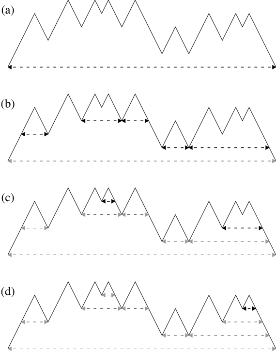
Figure 5: The drawing of baselines in a charge complex to determine its particle content. The small arrows indicate how to divide the $j$-th baseline into zeroth baselines of smaller complexes. (a) Drawing of the zeroth baseline. (b) Drawing of the first baseline. (c) Drawing of the second baseline. (d) Drawing of the third baseline.

    The result of this trivial step is shown in figure 5a for a typical charge complex.

  • Start from the highest point of the complex. If there is more than one highest point, start from the left-most highest point. Move down to the right of the peak along the contour of the complex till its endpoint. (The point were the next complex starts.) If a local minimum is reached, i.e., the contour of the complex starts going up again, we draw a dashed line from this local minimum to the right, until we cross the contour of the complex. At that point we move further down along the contour. If another minimum occurs we repeat the above, et cetera.

    We do exactly the same, now starting from the same left-most highest point but moving down to the left. If a local minimum is reached we draw a dashed line to the left and continue our movement down when the dashed line intersects the contour of the complex.

    The result of the above procedure is shown in figure 5b. The total of dashed line segments drawn in this step is called the first baseline.

  • We now view the first baseline as the zeroth baseline of smaller complexes. Let there be $L$ such smaller complexes. We then divide the first baseline into $L$ pieces by marking the begin- and endpoint of these complexes by arrows pointing to the left and right, respectively, see figure 5b.

    Either these complexes consist of a single particle (complexes with one maximum and consequently no local minima), or they are again complexes in the true sense of the word. In the latter case, we repeat the procedure of drawing dashed lines, again starting from the left-most highest point.

    The result of this third round of drawing dashed lines is shown in figure 5c. The total of dashed line drawn in this step is called the second baseline. Again this baseline is divided into pieces, marking yet smaller complexes.

  • We repeat the above procedure of drawing and cutting up higher order baselines iteratively. That is, we view the $j$-th baseline as the zeroth baseline of yet smaller objects, we draw arrows accordingly and, if some of these smaller complexes have more than one maximum, we start drawing the $(j+1)$-th baseline.

    Since the highest point of the complex is always less than $r-1$, the iteration terminates within $r-2$ steps (including the drawing of the zeroth baseline). In the case of figure 5, we are done in four iterative steps, figure 5d being the final result.

  • Given the complex with all the baselines we can read of its particle content straight away. First of all, according to R2, each peak corresponds to a particle. To determine its charge we move down vertically from its peak till me meet the zeroth baseline relative to this particle, i.e., we move down till we first intersect a baseline. The height of the peak minus the height of the baseline at the intersection point is its charge. In the example of figure 5d, we thus get $(n_{1},n_{2},\ldots)=(2,5,1,0,1,0,0,\ldots)$.

• Clearly we now determine the content of a given configuration as the sum of the particle content of all its complexes.

We note that in solving the problem of determining the particle content of a configuration we have actually localized each individual particle. Hence we can start moving the particles to the right to obtain the minimal configuration. We perform this motion in exactly the opposite order as described under M1-M6. Since our rules of motion are reversible (left-right invariant) we have consequently proven our assertion that each configuration can be obtained from a minimal configuration following the previously described rules.

A final ingredient needed in the Fermi gas is the actual Boltzmann weight of a given charge configuration. Given this we can try to compute the partition function. Before we describe this missing piece of information, let us first compute the total number of configurations keeping the particle content fixed, as this naturally leads us to introduce some final notation needed. Consider the particle of charge $j$ as shown in figure 6. We denote the left-most point of the particle its origin, and its right-most point its endpoint. All points $1,2,\ldots,2j-1$ will be referred to as interior points of the particle. Let us now ask the question in how many ways $I(j,k)$ this particle and the particle with charge $k<j$ shown in the same figure, can form a charge complex. Clearly, (see also figure 2), we can place the origin of the particle with charge $k$ at the following interior points of the particle of charge $j$:

$$2j-1,2j,\ldots,j+k.$$ (3.2)

Similarly, we can place the endpoint of the particle at the following interior points:

$$1,2,\ldots,j-k.$$ (3.3)

If we now remark that, according to rule R3, placing the origin at $j+k$ gives the same configuration as placing the endpoint at $j-k$, (see figure 2c and c’) we have a total of

$$I(j,k)=2j-2k-1$$ (3.4)

ways to form a complex of charge $j+k$.

This prepares us to answer the combinatorial question raised above. The number of ways to move the particles with charge $r-3$ to the left, starting from the minimal configuration, is

$$\sum_{k_{1}=0}^{2n_{r-2}}\sum_{k_{2}=0}^{k_{1}}\ldots\sum_{k_{n_{r-3}}=0}^{k_{n_{r-3}-1}}1=\left(2n_{r-2}+n_{r-3}\atop n_{r-3}\right),$$ (3.5)

since $I(r-3,r-4)=1$, and since we can position a particle not only in the interior of a larger particle as a charge complex, but also in between two larger particles as a separate unbound particle.

Similarly, the number of ways to move the particles with charge $r-4$ to the left is

$$\sum_{k_{1}=0}^{4n_{r-2}+2n_{r-3}}\sum_{k_{2}=0}^{k_{1}}\ldots\sum_{k_{n_{r-4}}=0}^{k_{n_{r-4}-1}}1=\left(4n_{r-2}+2n_{r-3}+n_{r-4}\atop n_{r-4}\right),$$ (3.6)

since $I(r-2,r-4)=3$ and $I(r-3,r-4)=1$. In the general case with particles of charge $j$ we obtain

$$\sum_{k_{1}=0}^{2(r-2-j)n_{r-2}+\ldots+4n_{j+2}+2n_{j+1}}\sum_{k_{2}=0}^{k_{1}}\ldots\sum_{k_{n_{j}}=0}^{k_{n_{j}-1}}1$$ (3.7)

$$\qquad\qquad\qquad\qquad=\left(2(r-2-j)n_{r-2}+\ldots+4n_{j+2}+2n_{j+1}+n_{j}\atop n_{j}\right),$$

as $I(r-2,j)=2(r-2-j)-1,\ldots,I(j+1,j)=1$. Of course the above calculation is rather clumsy, and we could have written the binomial answers straight away. As we later need the $q$-analogues of (3.5)-(3.7) we nevertheless thought it instructive to present the result in the above written form.

Collecting the above results we get for the total number of configurations $Z$ with fixed particle content $n_{1},n_{2}\ldots n_{r-2}$,

$$Z(n_{1},n_{2},\ldots,n_{r-2})=\prod_{j=1}^{r-3}\left(2\sum_{k=0}^{r-3-j}(r-2-j-k)n_{r-2-k}+n_{j}\atop n_{j}\right).$$ (3.8)

In turn summing over different particle content, computing the number of configurations $\Xi_{m}$ in a grand-canonical setting, we get

$$\Xi_{m}=\left.\sum_{n_{1},n_{2},\ldots,n_{r-2}\geq 0}\right.^{\!\!\!\!\!\!\!\!\!\!\!\!\!\!\!\!\!{}^{\prime}}\qquad Z(n_{1},n_{2},\ldots,n_{r-2}),$$ (3.9)

where the prime over the sum indicates the restriction (3.1), i.e., we sum over particle numbers keeping the size of the system fixed.

This last result suggests in fact to eliminate one degree of freedom. To do so we introduce the variables $m_{j}$ as the number of antiparticles of charge $-j$,

$$m_{j}=2n_{j+1}+4n_{j+2}+\ldots+2(r-2-j)n_{r-2},\qquad j=1,\ldots,r-2.$$ (3.10)

From this we see that antiparticles of charge $-(r-2)$ are absent, and hence we can eliminate the dependence on the particles of charge $r-2$. Using the vector notation $\vec{m}=(m_{1},m_{2},\ldots,m_{r-3})^{T}$, $\vec{n}=(n_{1},n_{2},\ldots,n_{r-3})^{T}$ and $(\vec{\mbox{e}}_{1})_{j}=\delta_{1,j}$, and denoting the incidence matrix of the A_r-3 Dynkin diagram as $\cal I$, we find

$$\vec{m}+\vec{n}=\frac{1}{2}\left({\cal I}\>\vec{m}+m\>\vec{\mbox{e}}_{1}\right),$$ (3.11)

and

$$\Xi_{m}=\left.\sum\right.^{{}^{\prime}}\;\prod_{j=1}^{r-3}\left(m_{j}+n_{j}\atop m_{j}\right).$$ (3.12)

Here the sum is over all (integer) solutions to the constraint equation (3.11), where the prime denotes the restriction to even antiparticle numbers $m_{j}$, as follows from (3.10). Equation (3.11), relating the variables $n_{j}$ to the new variables $m_{j}$, originates from the work on fermionic sums by Berkovich [12]. As we will see in section 5, it also appears in the context of TBA.

3.2 Computation of the partition function

We now finally come to the actual definition of the Boltzmann weight of a charge configuration, and to the calculation of the grand-canonical partition function.

Let us return to the charge configuration of figure 3. Clearly, at each (integer) point $x$ $(x=1,\ldots,m-1)$ of the lattice there are four possibilities for the contour of the configuration. We either have a straight line going up or down, or there is a cusp corresponding to a (local) minimum or maximum. We now assign an energy $E(x)$ to each site $x$ of the lattice by

$$-\beta E(x)=\left\{\begin{array}[]{ll}\frac{1}{2}x\log q&\mbox{if the contour at position $x$ is a straight line}\\ 0&\mbox{if the contour at position $x$ is a cusp.}\end{array}\right.$$ (3.13)

Clearly, with this definition the groundstate of the model is given by the state with only particles of charge 1. For given, fixed particle content, the energy is minimized by ordering the particles to form a minimal configuration.

The remainder of this subsection is devoted to the computation of the grand-canonical partition function of our Fermi gas,

$$\Xi_{m}(q)=\sum_{\mbox{\scriptsize particle content}}Z(n_{1},\ldots,n_{r-2};q),$$ (3.14)

with the partition function of fixed particle content given by

$$Z(n_{1},\ldots,n_{r-2};q)=\sum_{\mbox{\scriptsize charge configurations}}\mbox{e}^{\displaystyle-\beta\sum_{k=1}^{m-1}E(k)}.$$ (3.15)

To compute $Z$ we follow a procedure similar to that employed in the section 3.1. First we consider the minimal configuration, and from that we obtain all other configurations with equal content by carrying out the steps M1-M6. The only extra input will be that changing the position of a particle changes the energy of a configuration.

To compute the energy of a minimal configuration we proceed as follows. The energy of a particle with charge $j$, with its origin at position $x$ is

$$-\beta E(j,x)=\frac{1}{2}\log q\sum_{k=1,\;k\neq j}^{2j-1}(k+x)=(j+x)(j-1)\log q$$ (3.16)

Hence, for the minimal configuration with content $n_{1},\ldots,n_{r-2}$ we compute

$$-\beta E_{\mbox{\scriptsize min}} = \log q\sum_{j=1}^{r-2}\sum_{\ell=1}^{n_{j}}E\left(j,2j(\ell-1)+2\sum_{k=j+1}^{r-2}k\,n_{k}\right)$$

$$= \log q\sum_{j=1}^{r-2}(j-1)n_{j}\left(j\,n_{j}+2\sum_{k=j+1}^{r-2}k\,n_{k}\right)$$

$$= \log q\sum_{j=1}^{r-3}\sum_{k=1}^{r-3}n_{j+1}\,A_{j,k}\,n_{k+1},$$

with matrix $A$ defined as

$$A_{j,k}=\left\{\begin{array}[]{ll}j(k+1)&j\leq k\\ A_{k,j}&j>k.\end{array}\right.$$ (3.18)

Writing this in favour of the occupation numbers of antiparticles $m_{j}$ defined in (3.10), we can simplify to

$$\mbox{e}^{\displaystyle-\beta E_{\mbox{\scriptsize min}}}=q^{\displaystyle{\textstyle{1\over 4}}\>\vec{m}^{T}C\>\vec{m}},$$ (3.19)

where $C$ denotes the Cartan matrix of the simply-laced Lie algebra A_r-3.

As before, all other states with the same content $n_{1},\ldots,n_{r-2}$ are obtained from the minimal configuration by moving particles to the left following M1-M6. The combinatorics of this rearranging of particles has been considered in section 3.1. What has not yet been worked out is the increase of energy associated with the leftward motion of a particle. Since we move one particle at a time, we only have to calculate the energy increase of the movement of a particle of charge $k$, relative to a charge complex with charge $j>k$ positioned immediately to the left of this particle. Possibly the simplest way to go about is to first view the complex and the particle as one single complex with charge $j+k$. Suppose that relative to the origin of this complex we have (local) minima and maxima of the contour at $0<x_{1}<y_{1}<x_{2}<y_{2}<\ldots<x_{n-1}<y_{n-1}<x_{n}<2k+2j$, labelling minima by $y$ and maxima by $x$. Note that the simplest possible scenario; the complex of charge $j$ consisting of a single particle, corresponds to $n=2$. The total weight of the complex relative to its own origin is thus

$$\sum_{\begin{array}[]{c}\ell=1\\ \ell\neq x_{i},y_{i}\end{array}}^{2j+2k-1}q^{k/2}.$$ (3.20)

Now start moving the particle with charge $k$ one step to the left, like shown in figure 2. This results in a decrease of both $y_{n-1}$ and $x_{n}$ by 1. The weight increase of this step is hence a factor

$$\frac{q^{(y_{n-1}+x_{n}+2)/2}}{q^{(y_{n-1}+x_{n})/2}}=q.$$ (3.21)

Taking another step to the left, again leads to a decrease of $y_{n-1}$ and $x_{n}$ by 1 and we pick up another factor $q$. This process can be repeated until $y_{n-1}-x_{n-1}=x_{n}-y_{n-1}$, corresponding to the situation that the maxima at $x_{n}$ and $x_{n-1}$ have equal height (see figure 2c). From then on moving the particle a single step leads to a decrease of $x_{n-1}$ and $y_{n-1}$ by 1. However, this still leads to an increase by a single factor $q$, and we are led to conclude that each step of particle $k$ trough the complex yields an extra factor $q$.

With this result we can simply carry out the $q$-analogue of the previous subsection. To do so we repeatedly make use of the identity [29]

$$\sum_{k_{1}=0}^{N}\sum_{k_{2}=0}^{k_{1}}\ldots\sum_{k_{M}=0}^{k_{M-1}}q^{k_{1}+k_{2}+\ldots+k_{M}}=\left[N+M\atop M\right]_{q}.$$ (3.22)

First we start moving the particles of charge $r-3$ by (3.22) this gives a Boltzmann factor

$$\sum_{k_{1}=0}^{2n_{r-2}}\sum_{k_{2}=0}^{k_{1}}\ldots\sum_{k_{n_{r-3}}=0}^{k_{n_{r-3}-1}}q^{k_{1}+k_{2}+\ldots+k_{n_{r-3}}}=\left[2n_{r-2}+n_{r-3}\atop n_{r-3}\right]_{q}=\left[n_{r-3}+m_{r-3}\atop m_{r-3}\right]_{q}.$$ (3.23)

Similarly, moving the particles with charge $r-4$ to the left results in

$$\sum_{k_{1}=0}^{4n_{r-2}+2n_{r-3}}\sum_{k_{2}=0}^{k_{1}}\ldots\sum_{k_{n_{r-4}}=0}^{k_{n_{r-4}-1}}q^{k_{1}+k_{2}+\ldots+k_{n_{r-4}}}=\left[4n_{r-2}+2n_{r-3}+n_{r-4}\atop n_{r-4}\right]_{q}=\left[n_{r-4}+m_{r-4}\atop m_{r-4}\right]_{q}.$$ (3.24)

In the general case of particles with charge $j$ we end up with the contribution

$$\sum_{k_{1}=0}^{2(r-2-j)n_{r-2}+\ldots+4n_{j+2}+2n_{j+1}}\sum_{k_{2}=0}^{k_{1}}\ldots\sum_{k_{n_{j}}=0}^{k_{n_{j}-1}}q^{k_{1}+k_{2}+\ldots+k_{n_{j}}}$$ (3.25)

$$\qquad\qquad=\left[2(r-2-j)n_{r-2}+\ldots+4n_{j+2}+2n_{j+1}+n_{j}\atop n_{j}\right]_{q}=\left[n_{j}+m_{j}\atop m_{j}\right]_{q}.$$

From the results (3.23)-(3.25) and (3.19) we obtain an expression for the partition function $Z$ as

$$Z(n_{1},n_{2},\ldots,n_{r-2};q)=q^{\textstyle\frac{1}{4}\>\vec{m}^{T}C\>\vec{m}}\prod_{j=1}^{r-3}\left[m_{j}+n_{j}\atop m_{j}\right]_{q},$$ (3.26)

with equations (3.10) and (3.11) relating the antiparticle numbers $m_{j}$ to the particle numbers $n_{j}$. We can finally end this section by stating the result for the grand-canonical partition function,

$$\Xi_{m}(q)=\sum_{\mbox{\scriptsize particle content}}Z(n_{1},n_{2},\ldots,n_{r-2};q)=\left.\sum\right.^{{}^{\prime}}\;q^{\textstyle\frac{1}{4}\>\vec{m}^{T}C\>\vec{m}}\prod_{j=1}^{r-3}\left[m_{j}+n_{j}\atop m_{j}\right]_{q},$$ (3.27)

where, as in (3.12), the second sum is over all solutions to (3.11) with each entry of $\vec{m}$ being even.

3.3 Mapping of configuration sums onto Fermi gas partition function

To show that the result (3.27) is indeed the evaluation of (2.15) with $a=b=1$ and $c=2$, we fix the spins $\sigma_{j}\in\{1,2,\ldots,r-1\}$ such that $|\sigma_{j+1}-\sigma_{j}|=1$ for all $j$, and such that $\sigma_{0}=\sigma_{m}=1,\;\sigma_{m+1}=2$. We call such a sequence $(\sigma_{0},\sigma_{1},\ldots,\sigma_{m+1})$ admissible. Next we plot $\sigma_{j}$ as a function of $j$ and interpolate between $(j,\sigma_{j})$ and $(j+1,\sigma_{j+1})$ by a straight line. We call the graph thus obtained the contour of $(\sigma_{0},\ldots,\sigma_{m+1})$. A typical contour of an admissible sequence of sigma’s is shown in figure 7. From the definition (2.15) of the configuration sums we see that a straight line segment through $(j,\sigma_{j})$, corresponding to $|\sigma_{j-1}-\sigma_{j+1}|=2$, yields a factor $q^{j/2}$. The total weight of an admissible sequence can therefore be written as

$$\mbox{e}^{\displaystyle-\beta\sum_{j=1}^{m-1}E(j)}$$ (3.28)

where the energy function $E(j)$ is precisely that of the Fermi gas given by equation (3.13). Since summing over all admissible sequences corresponds to summing over all contours, which in turn corresponds to summing over all charge configuration, we have established the desired equivalence.

We note that particle-like interpretations of admissible contours (or paths) have been previously formulated for the minimal conformal series M$(2,k)$ in refs. [31-33].

The above equivalence also explains the defining rules R1 and R3. From (2.15) we have to count each admissible sequence of spins just once. However, interchanging two identical particles leads to the same contour, and would therefore lead to multiple counting of one and the same admissible sequence. Similarly we have to impose R3 to avoid overcounting of admissible sequences.

At the same time the mapping explains why the particular choice of $X_{m}(1,1,2)$ is simplest to evaluate using the fermionic technique. If for e.g., we take $a>1$, we have to introduce a particle, which, in separated unbound form, would have a profile of a single straight line going down. This boundary particle has a (fractional) charge of $(a-1)/2$. Similarly, when $b=c-1>1$ we need a boundary particle of charge $b/2$ with profile of a straight line going up. These particles are in contrast with the particles introduced so far, which have origin and endpoint of equal height. Since the motion of a (bulk)particle through a boundary particle is very different from that defined in R2 on page R2, the general $X_{m}(a,b,c)$ case becomes quite complicated and technical. For this reason the computation of all one-dimensional configuration sums will be deferred to part II.

4 Polynomial and Rogers–Ramanujan type identities

Since the bosonic and the fermionic method to evaluate the configuration sum $X_{m}(1,1,2)$ yield rather different type of expressions, we can of course combine results to find some nontrivial identities. Setting $a=b=1$ and $c=2$ in (2.22), substituting (3.11) into (3.27), and replacing $m$ by $2m$, yields

$$\sum_{\begin{array}[]{c}\scriptstyle m_{1},\ldots,m_{r-3}\geq 0\\ \scriptstyle\vec{m}\in 2\mbox{\scriptsize\sf Z}\!\!\mbox{\scriptsize\sf Z}^{r-3}\end{array}}q^{{\textstyle{1\over 4}}\>\textstyle\vec{m}^{T}C\>\vec{m}}\prod_{j=1}^{r-3}\left[{\textstyle{1\over 2}}({\cal I}\>\vec{m})_{j}+m\delta_{j,1}\atop m_{j}\right]_{q}$$ (4.4)

$$\qquad=\sum_{j=-\infty}^{\infty}\left\{q^{r(r-1)j^{2}+j}\left[2m\atop m-rj\right]_{q}-q^{r(r-1)j^{2}+(2r-1)j+1}\left[2m\atop m-1-rj\right]_{q}\right\}.$$

These identities are precisely the polynomial identities for $X_{2m}(1,1,2)$ as conjectured by Melzer in ref. [10]. A different proof of (4.4) has been published by Berkovich [12]. In his proof Berkovich has shown that a larger class of fermionic expressions, corresponding to all $X_{m}(1,b,b\pm 1)$ solves the same recurrences (2.19) as the bosonic expressions (2.22) of ABF. To establish this, elegant generalizations of the decompositions (2.23) for the $q$-binomials were used. One of the great merits of the recursive proof of ref. [12] is that it proves a whole set of fermionic expressions at the same time, and that complications with the boundary for general $X_{m}(a,b,c)$ are avoided [34]. On the other hand, the proof as given in this paper has the advantage of providing detailed information relating BA solutions (see next section), admissible sequences of spins occurring in the CTM calculation, charge configurations of the Fermi gas and actual terms within the sum on the left-hand side of (4.4).

In taking the $m\to\infty$ limit of (4.4), using $\lim_{m\to\infty}\left[{\textstyle{m\atop k}}\right]_{q}=1/(q)_{k}$ and $\lim_{m\to\infty}\left[{\textstyle{2m\atop m}}\right]_{q}=1/(q)_{\infty}$, the following Rogers–Ramanujan type identities for the $X_{1,1}^{(r-1,r)}(q)$ Virasoro characters arise:

$$\sum_{\begin{array}[]{c}\scriptstyle m_{1},\ldots,m_{r-3}\geq m_{r-2}\equiv 0\\ \scriptstyle\vec{m}\in 2\mbox{\scriptsize\sf Z}\!\!\mbox{\scriptsize\sf Z}^{r-3}\end{array}}\frac{q^{{\textstyle{1\over 4}}\>\textstyle\vec{m}^{T}C\>\vec{m}}}{(q)_{m_{1}}}\prod_{j=2}^{r-3}\left[{\textstyle{1\over 2}}(m_{j-1}+m_{j+1})\atop m_{j}\right]_{q}$$ (4.8)

$$\qquad\qquad\qquad\qquad\qquad=\frac{1}{(q)_{\infty}}\sum_{j=-\infty}^{\infty}\left\{q^{r(r-1)j^{2}+j}-q^{r(r-1)j^{2}+(2r-1)j+1}\right\}.$$

These identities were first conjectured by the Stony Brook group in ref. [11].

To obtain Rogers–Ramanujan type identities for the branching functions of the $\;\>\mbox{\sf Z}\mbox{\sf Z}\,_{r-2}$ parafermion conformal field theories of ref. [35], we replace $q$ by $1/q$ in (4.4) and again let $m\to\infty$. This results in

$$\sum_{\begin{array}[]{c}\scriptstyle m_{1},\ldots,m_{r-3}\geq 0\\ \scriptstyle(C^{-1}\vec{m})_{r-3}\in\mbox{\scriptsize\sf Z}\!\!\mbox{\scriptsize\sf Z}\end{array}}\frac{q^{\textstyle\vec{m}^{T}C^{-1}\>\vec{m}}}{(q)_{m_{1}}\ldots(q)_{m_{r-3}}}$$ (4.12)

$$\qquad\qquad\qquad=\frac{q^{-{\textstyle{(r-3)(r-2)\over 24r}}}}{[(q)_{\infty}]^{r-3}}\sum_{\alpha\in Q}\sum_{w\in W}\mbox{sgn}(w)\;q^{\displaystyle{\textstyle{1\over 2}}r(r-1)\left|\alpha-\frac{r\rho-(r-1)w(\rho)}{r(r-1)}\right|^{2}}\;,$$

with $Q$ the root lattice, $W$ the Weyl group and $\rho$ the Weyl vector of A_r-3. We note that the left-hand side of these identities are the expressions for the branching functions obtained by Lepowsky and Primc [36]. To derive the above we have used the level-rank equivalence between the $(r-1)$-state ABF model in regime III and the level-2 A_r-3 Jimbo-Miwa-Okado model in regime II [17], to rewrite the SU(2) type right-hand side of (4.4) into an SU($r-2$) type form [24] (see also the discussion in ref. [25]). For $r=4$ we note that (4.8) and (4.12) coincide.

5 CTM versus TBA

The reader familiar with the TBA computations for the ABF model of Bazhanov and Reshetikhin (BR) [4], will have noticed the many similarities between the TBA and the Fermi gas. This section serves to indeed show the mathematical equivalence between the fermionic CTM calculations of section 3 and the TBA calculations of ref. [4].

First let us recall the Bethe Ansatz equations for the ABF model [4, 5]

$$\omega^{2}\left(\frac{\vartheta_{1}(\frac{1}{2}\lambda+\,\mbox{i}\,\alpha_{j})}{\vartheta_{1}(\frac{1}{2}\lambda-\,\mbox{i}\,\alpha_{j})}\right)^{m}=-\prod_{k=1}^{m/2}\frac{\vartheta_{1}(\,\mbox{i}\,\alpha_{j}-\,\mbox{i}\,\alpha_{k}+\lambda)}{\vartheta_{1}(\,\mbox{i}\,\alpha_{j}-\,\mbox{i}\,\alpha_{k}-\lambda)},\qquad j=1,\ldots,{\textstyle{1\over 2}}m.$$ (5.1)

Here $\omega=\exp(\,\mbox{i}\,\ell\lambda),$ $\ell=1,\ldots,r-1$, $\lambda=\pi/r$ and each set of roots $\{\alpha_{1},\ldots,\alpha_{m/2}\}$ yields an eigenvalue $\Lambda(u)$ of the row-to-row transfer matrix.

Based on exact information for the cases $r=3$ (trivial 2-state model) and $r=4$ (Ising model), and on a numerical investigation for other $r$ values, BR formulated the following string hypothesis: For $m\to\infty$ all solutions to the BAE consist of sets of strings, with the allowed string types given by

$$\alpha_{\mu}^{(j)}=\alpha^{(j)}-\frac{\,\mbox{i}\,\pi}{2r}(j+1-2\mu)\qquad\mu=1,\ldots,j;\qquad j=1,\ldots,r-2,$$ (5.2)

where $\mu$ labels the $j$ roots within a string and $j$ the different types of strings. The real variable $\alpha^{(j)}$ is the string center.

As described in the introduction, we define our finitized model by assuming the string hypothesis to be correct for finite $m$. Let $n_{j}$ denote the number of strings of type $j$. Then, since the total number of roots in a solution equals ${\textstyle{1\over 2}}m$, we have the completeness relation

$$\sum_{j=1}^{r-2}j\,n_{j}={\textstyle{1\over 2}}m.$$ (5.3)

We note this is exactly the completeness relation (3.1) for the particle numbers of the Fermi gas.

Substituting the hypothesis into the finite $m$ BAE, a set of reduced equations is obtained which only involve the string centers. Carrying out the standard TBA procedures [4, 37, 21], the reduced equations yield the following set of constraint equations for the number of strings $n_{j}$ and the number of holes $m_{j}$ (counting the missing Takahashi numbers):

$$m\,b_{j}=m_{j}+\sum_{k=1}^{r-2}B_{j,k}\,n_{k},$$ (5.4)

with

$$B_{j,k}=\left\{\begin{array}[]{ll}\frac{\displaystyle 2(r-j)k}{\displaystyle r}&j\geq k\\ B_{k,j}&j<k\end{array}\right.,\qquad\qquad b_{j}=\frac{r-j}{r}.$$ (5.5)

Following BR we set $j=r-2$ in (5.4) to find $m_{r-2}=0$. Now eliminating $n_{r-2}$ yields precisely the constraint equation (3.11), and we conclude that we can identify the strings (holes) of type $j$ with the particles (antiparticles) of charge $j$ $(-j)$ of the Fermi gas. In other words, with each solution to the BAE for the finitized model corresponds a configuration of the Fermi gas, and vice versa. We remark here that we can in fact easily establish a bijection between Bethe Ansatz solutions and Coulomb gas configurations. So, for e.g., minimal configurations in the Fermi gas correspond to solutions without holes, and the leftward motion of a particle with charge $j$ corresponds to shifting the Takahashi numbers $I^{(j)}$ by “inserting” numbers $\tilde{I}^{(j)}$ corresponding to the creation of holes. Using the map from the Fermi gas configurations to the configuration sums, we have in fact a bijection between admissible sequences of spins $(\sigma_{1},\ldots,\sigma_{m+1})$ and solutions to the Bethe Ansatz equations labelled by their Takahashi numbers. In this context we should mention that several authors [37, 19, 12, 21] have indeed conjectured and/or computed the total number of solutions to the Bethe equations to be expression (3.12), here counting the number of charge configurations in the Fermi gas.

To further obtain the equations of TBA, we first let $m\to\infty$ in the Fermi gas partition function (3.27), and then take the limit $q\to 1^{-}$. This procedure, developed in refs. [38, 39], is equivalent to computing the $T\to 0$ asymptotics of the entropy in TBA. Writing $\lim_{m\to\infty}\Xi_{m}(q)=\sum_{k}a_{k}q^{k}$, we have the asymptotics

$$\log a_{k}\sim\sqrt{3\pi\left.\frac{S(T)}{T}\right|_{T=0}}\quad.$$ (5.6)

Computing $a_{k}$ by steepest descend gives us [15]

$$S(T)=-\frac{8\,T}{\pi}\sum_{j=1}^{r-3}[L(\xi_{j})-L(\eta_{j})]+o(T),$$ (5.7)

with $L$ the Rogers dilogarithm function [40]

$$L(z)=\frac{1}{2}\int_{0}^{z}\left[\frac{\log(1-\zeta)}{\zeta}+\frac{\log\zeta}{1-\zeta}\right]\mbox{d}\zeta.$$ (5.8)

The numbers $\xi_{j}$ follow from the TBA equations [4],

$$2\log(1-\xi_{j})=\sum_{k=1}^{r-3}C_{j,k}\,\log(\xi_{k}),$$ (5.9)

which arise here as the conditions for the saddle point. The $\eta_{j+1}$ follow from the TBA equations with $r$ replaced by $r-1$, and $\eta_{1}=1$.

Using the identity [41]

$$\sum_{j=1}^{r-3}[L(\xi_{j})-L(\eta_{j})]=-\frac{\pi^{2}}{6}\left(1-\frac{6}{r(r-1)}\right),$$ (5.10)

we finally get

$$\left.\frac{S(T)}{T}\right|_{T=0}=\frac{4\pi}{3}\left(1-\frac{6}{r(r-1)}\right),$$ (5.11)

in accordance with the TBA result of BR. From this last result the central charge of the ABF models can be read off as [42]

$$c=1-\frac{6}{r(r-1)}.$$ (5.12)

To conclude this section, we wish to make a comment on the TBA calculations of BR as carried out in ref. [4]. One of the shortcomings of their calculation is the failure to also derive results for the scaling dimensions of the ABF model. However, from the equivalence between the Fermi gas and the TBA approach, it is clear that the constraint equations (3.11) which follow from the string hypothesis (5.2) only describe the vacuum or groundstate sector of the model. As argued before, to compute other configuration sums than $X_{m}(1,1,2)$, (which corresponds to computing scaling dimensions) additional boundary particles have to be introduced on top of the Fermi gas. These extra particles result in a modification of the constraint equations (3.11). We therefore believe that the string hypothesis as formulated by BR is incomplete and does not describe all solutions to the BAE. Indeed, the total number of eigenvalues of the row-to-row transfer matrix of the ABF model exceeds the number of configurations of the Fermi gas. The fractional structure of the additional boundary particles needed for the general configuration sums, seems to suggest the existence of half-strings, which have roots in the upper or lower part of the complex plane only.

6 Summary and discussion

In this paper we have presented a new method for computing the one-dimensional configuration sums of the ABF model in regime III. Our approach, based on the interpretation of the configuration sums as the grand-canonical partition function of a one-dimensional gas of charged fermions, results in polynomial expressions of fermionic type. This opposed to the bosonic polynomials obtained by employing the recurrence method of Andrews, Baxter and Forrester [9]. Combining both bosonic and fermionic techniques leads to a proof of Melzer’s polynomial identities [10], different from the recursive proof by Berkovich [12]. In taking the thermodynamic limit, this also proofs the Rogers–Ramanujan identities for unitary minimal Virasoro characters as conjectured by Kedem et al. [11]. Since our fermionic method is mathematically equivalent to the thermodynamic Bethe Ansatz calculations for the ABF model of Bazhanov and Reshetikhin [4], we have established a unification of the corner transfer matrix and of the TBA technique. Here it is to be noted that in our calculations the particle content of the model follows without making the usual string hypothesis characterizing TBA calculations.

Although we have applied our method to the simplest possible configuration sum of the ABF model, the other sums can be computed be introducing additional boundary particles to the Fermi gas. The details of this procedure will be treated in part II of this paper [44]. What is more, our method is by no means restricted to the ABF model, and we believe that all restricted solid-on-solid models for which the TBA program has been carried out [4, 5, 6, 45, 46] admit a fermionic computation of their configuration sums. We thus hope that our approach leads to proofs of the many polynomial and Rogers–Ramanujan identities conjectured in the recent literature [16, 11, 24, 26].

We also note that our Fermi gas formulation of the ABF configuration sums can be reformulated to obtain a partition theoretic proof of Melzer’s identities. Such a proof corresponds to establishing a bijection between partitions with prescribed hook differences [47] and charge configurations of the Fermi gas. Work on this bijection is currently in progress in collaboration with O. Foda [48].

Finally, it would be extremely interesting to connect the approach to fermionic character representations of Bouwknegt et al. [49-51] using Yangian symmetries, and of Georgiev using vertex operators [52], to that of this paper.

Figure 1: A possible charge configuration of the Coulomb gas for $r\geq 7$.

Figure 2: The movement of a particle of charge $k$ through a particle of charge $j>k$. According to rule R3 the configurations in figure c and c’ are to be identified. The dashed lines are the baselines as described on page 8. We note that the procedure for drawing the baselines in fact rules out possibility c’ thus avoiding overcounting of configurations.

Figure 3: A typical charge configuration in which some of the particles have formed charge complexes.

Figure 4: The construction of the charge configuration of figure 3 out of a minimal configuration by carrying out the steps described under M1-M6.

Figure 6: Particles of charge $j$ and $k$ with labelling of begin-, end- and interior points.

Figure 7: A contour of a typical admissible sequence of spins $(\sigma_{0},\sigma_{1},\ldots,\sigma_{m+1})$.

References

- [1] C. N. Yang and C. P. Yang, J. Math. Phys. 10:1115 (1969).
- [2] M. Takahashi, Prog. Theor. Phys. 46:401 (1971).
- [3] M. Takahashi and M. Suzuki, Prog. Theor. Phys. 48:2187 (1972).
- [4] V. V. Bazhanov and N. Yu Reshetikhin, Int. J. Mod. Phys. A 4:115 (1989).
- [5] V. V. Bazhanov and N. Yu Reshetikhin, J. Phys. A: Math. Gen. 23:1477 (1990).
- [6] V. V. Bazhanov and N. Yu Reshetikhin, Prog. Theor. Phys. 102:301 (1990).
- [7] R. J. Baxter, Exactly solved models in statistical mechanics (Academic Press, London, 1982).
- [8] G. Albertini, S. Dasmahapatra and B. M. McCoy, Int. J. Mod. Phys. A 7, Suppl. 1A:1 (1992).
- [9] G. E. Andrews, R. J. Baxter and P. J. Forrester, J. Stat. Phys. 35:193 (1984).
- [10] E. Melzer, Int. J. Mod. Phys. A 9:1115 (1994).
- [11] R. Kedem, T. R. Klassen, B. M. McCoy and E. Melzer, Phys. Lett. 304B:263 (1993).
- [12] A. Berkovich, Nucl. Phys. B 431:315 (1994).
- [13] R. Kedem and B. M. McCoy, J. Stat. Phys. 71:883 (1993).
- [14] S. Dasmahapatra, R. Kedem, B. M. McCoy and E. Melzer, J. Stat. Phys. 74:239 (1994).
- [15] S. Dasmahapatra, R. Kedem, T. R. Klassen, B. M. McCoy and E. Melzer, Int. J. Mod. Phys. B 7:3617 (1993).
- [16] R. Kedem, T. R. Klassen, B. M. McCoy and E. Melzer, Phys. Lett. 307B:68 (1993).
- [17] M. Jimbo, T. Miwa and M. Okado, Nucl. Phys. B 300 [FS22]:74 (1988).
- [18] A. Kuniba, T. Nakanishi and J. Suzuki, Mod. Phys. Lett. A 8:1649 (1993).
- [19] S. Dasmahapatra, String hypothesis and characters of coset CFT’s preprint ICTP IC/93/91, hep-th/9305024.
- [20] E. Melzer, Lett. Math. Phys. 31:233 (1994).
- [21] S. Dasmahapatra, On State Counting and Characters preprint CMPS 94-103, hep-th/9404116.
- [22] O. Foda and Y.-H. Quano, Polynomial identities of the Rogers–Ramanujan type preprint University of Melbourne No. 25-94, hep-th/9407191.
- [23] S. O. Warnaar and P. A. Pearce, J. Phys. A: Math. Gen. 27:L891 (1994).
- [24] S. O. Warnaar and P. A. Pearce, A-D-E Polynomial and Rogers–Ramanujan Identities, preprint University of Melbourne No. 41-94, hep-th/9411009.
- [25] A. Berkovich and B. M. McCoy, Continued Fractions and Fermionic Representations for Characters of Minimal Models, preprint BONN-TH-94-28, ITPSB 94-060, hep-th/9412030.
- [26] E. Melzer, Supersymmetric Analogs of the Gordon–Andrews Identities, and related TBA Systems, preprint TAUP 2211-94, hep-th/9412154.
- [27] D. A. Huse, Phys. Rev. Lett. 49:1121 (1982).
- [28] R. J. Baxter, J. Stat. Phys 26:427 (1981).
- [29] G. E. Andrews, The Theory of Partitions (Addison-Wesley, Reading, Massachusetts, 1976).
- [30] A. Rocha-Caridi, in Vertex Operators in Mathematics and Physics, eds. J. Lepowsky, S. Mandelstam and I. M. Singer (Springer, Berlin, 1985).
- [31] D. Bressoud, Lecture Notes in Math. 1395:140 (1987).
- [32] J. Kellendonk, M. Rösgen and R. Varnhagen, Int. J. Mod Phys. A 9:1009 (1994).
- [33] M. Rösgen and R. Varnhagen, Steps towards Lattice Virasoro Algebras: su(1,1) preprint BONN-TH-94-23, hep-th/9501005.
- [34] A. Berkovich, private communication.
- [35] A. B. Zamolodchikov and V. A. Fateev, Sov. Phys. JETP 62:215 (1985).
- [36] J. Lepowsky and M. Primc, Structure of the standard modules for the affine Lie algebra A Contemporary Mathematics, 46 (AMS, Providence, 1985).
- [37] A. Berkovich, C. Gomez and G. Sierra, Nucl. Phys. B 415:681 (1994).
- [38] B. Richmond and G. Szekeres, J. Austral. Math. Soc. (A) 31:362 (1981).
- [39] W. Nahm, A. Recknagel and M. Terhoeven, Mod. Phys. Lett. A 8:1835 (1993).
- [40] L. Lewin, Polylogarithms and Associated Functions (Elsevier, Amsterdam, 1981).
- [41] A. N. Kirillov and N. Yu. Reshetikhin, J. Sov. Math. 52:3156 (1990).
- [42] I. Affleck, Phys. Rev. Lett. 56:746 (1986).
- [43] V. V. Bazhanov, S. L. Lukyanov, A. B. Zamolodchikov, Integrable Structure of Conformal Field Theory, Quantum KdV Theory and Thermodynamic Bethe Ansatz, preprint CLNS 94/1316, hep-th/9412229.
- [44] S. O. Warnaar, Fermionic solution of the Andrews-Baxter-Forrester model II: proof of Melzer’s polynomial identities, in preparation.
- [45] A. Kuniba, Nucl. Phys. B 389:209 (1993).
- [46] V. V. Bazhanov, B. Nienhuis and S. O. Warnaar, Phys. Lett. 322B:198 (1994).
- [47] G. E. Andrews, R. J. Baxter, D. M. Bressoud, W. J. Burge, P. J. Forrester and G. Viennot, Europ. J. Comb. 8:341 (1987).
- [48] O. Foda and S. O. Warnaar, Bijective proof of Melzer’s polynomial identities: the case, preprint University of Melbourne No. 03-95.
- [49] P. Bouwknegt, A. W. W. Ludwig and K. Schoutens, Phys. Lett. 338B:448 (1994).
- [50] P. Bouwknegt, A. W. W. Ludwig and K. Schoutens, Spinon basis for higher level SU(2) WZW models, preprint USC-94/20, hep-th/9412108.
- [51] P. Bouwknegt, A. W. W. Ludwig and K. Schoutens, Affine and Yangian symmetries in conformal field theory, preprint USC-94/21, hep-th/9412199.
- [52] G. Georgiev, Combinatorial construction of modules for infinite-dimensional Lie algebras, I. Principal subspace, preprint Rutgers University, hep-th/9412054.