Correlation Functions in Matrix Models
Modified by Wormhole Terms

Abstract

We calculate correlation functions in matrix models modified by trace-squared terms. First we study scaling operators in modified one-matrix models and find that their correlation functions satisfy modified Virasoro constraints. Then we turn to dressed order parameters in minimal models and show that their correlators satisfy Goulian-Li formulae continued to negative Liouville dressing exponents. Our calculations provide additional support for the idea that the modified matrix models contain operators with the negative branch of gravitational dressing.

1 Introduction

In recent literature some effort has been devoted to studying the large $N$ matrix models modified by trace-squared terms  [?,?,?,?,?,?,?,?]. In the one-matrix models, for instance, one may add terms like $g({\rm Tr\,}\Phi^{4})^{2}$ to the conventional matrix potential of the form $N{\rm Tr\,}V(\Phi)$.

Discretized random surfaces appear in the Feynman graph expansion of the matrix models, and the vertex corresponding to the trace-squared term may be thought of as an identification between a pair of ordinary plaquettes. If the two plaquettes belong to otherwise disconnected random surfaces, then this identification introduces a tiny “neck” into the geometry; if they belong to the same connected component, then the identification attaches a microscopic handle. These two types of effects are familiar consequences of the Euclidean wormholes, which were widely explored in the four-dimensional quantum gravity. Thus, trace-squared terms are a convenient trick for adding wormholes to the random surface geometry, with the correct combinatorics emerging automatically. Actually, wormholes are known to be abundant already in conventional random surface theories with no trace-squared terms  [?,?,?]. Therefore, turning on the coupling $g$ does not introduce any new types of geometry into the path integral, but simply increases the weight of microscopic wormhole configurations. For example, in the sum over surfaces of genus zero there are geometries corresponding to trees of smooth spheres glued pairwise at single plaquettes, and increasing $g$ enhances their weight. It is not surprising, therefore, that a small increase in $g$ does not change the universal properties of the model. If, however, $g$ is fine-tuned to a finite positive value $g_{t}$, then the universality class of the large area behavior changes. For pure gravity ($c=0$) the string susceptibility exponent jumps from $-1/2$ for $g<g_{t}$ to $1/3$ for $g=g_{t}$. This is the simplest example of a matrix model where new critical behavior occurs due to fine-tuned wormhole weights.

Further work has revealed that, more generally, as the trace-squared coupling is increased to a critical value $g_{t}$, the string susceptibility exponent jumps from some negative value $\gamma$, found in a conventional matrix model, to a positive value

$$\bar{\gamma}={\gamma\over\gamma-1}\ .$$ (1.1)

Essentially equivalent results have been obtained without using matrix models, on the basis of direct combinatorial analysis  [?]. For a long time the positive values of string susceptibility exponent seemed very puzzling. Recently, however, a simple continuum explanation of these critical behaviors was proposed in ref.  [?].

For all the conventional matrix models describing $(p,q)$ minimal models coupled to gravity, the correct scaling follows from the Liouville action of the form

$$S_{L} = {1\over 8\pi}\int{\rm d}^{2}\sigma\,\left((\partial_{\mu}\phi)^{2}-Q\hat{R}\phi+tO_{\min}{\rm e}^{\alpha_{+}\phi}\right)\ ,$$

$$\alpha_{+} = {1\over 2\sqrt{3}}\left(\sqrt{1-c+24h_{\min}}-\sqrt{25-c}\right)=-{p+q-1\over\sqrt{2pq}}\ ,$$ (1.2)

where $O_{\min}$ is the matter primary field of the lowest dimension. A simple calculation reveals that the string susceptibility exponent is given by

$$\gamma=2+{Q\over\alpha_{+}}\ ,$$ (1.3)

where $Q=\sqrt{25-c\over 3}$. In ref.  [?] it was argued that the effect of fine-tuning the touching interaction is to replace the positively dressed Liouville potential by the negatively dressed one,

$$S_{L} = {1\over 8\pi}\int{\rm d}^{2}\sigma\,\left((\partial_{\mu}\phi)^{2}-Q\hat{R}\phi+\bar{t}O_{\min}{\rm e}^{\alpha_{-}\phi}\right)\ ,$$

$$\alpha_{-} = -{1\over 2\sqrt{3}}\left(\sqrt{1-c+24h_{\min}}+\sqrt{25-c}\right)=-{p+q+1\over\sqrt{2pq}}\ .$$ (1.4)

Now the string susceptibility exponent is found to be

$$\bar{\gamma}=2+{Q\over\alpha_{-}}={\gamma\over\gamma-1}\ ,$$ (1.5)

in agreement with the matrix model results. The intuitive reason for the change of the branch of gravitational dressing is that the microscopic wormholes alter the ultraviolet (large $\phi$) behavior of the theory. A priori, there are two independent solutions to the string equations of motion, corresponding to the two choices of dressing. The linear combination that appears in the theory is selected by the boundary conditions, and by fine-tuning the boundary conditions at large $\phi$ we have changed the string background.

A more complete understanding of the modified matrix models was recently found in ref.  [?]. As the trace-squared coupling is set to $g_{t}$ one finds the following non-perturbative relation

$${\rm e}^{\bar{F}(\bar{t};t_{1},t_{2},\ldots,t_{n})}=\int_{-\infty}^{\infty}{\rm d}t\,{\rm e}^{t\bar{t}+F(t;t_{1},t_{2},\ldots,t_{n})}\ ,$$ (1.6)

where $\bar{F}$ and $F$ are the universal parts of the modified and conventional free energies, respectively. As indicated in eqs. (1) and (1), $t$ is the lowest dimension coupling in the conventional action and $\bar{t}$ is the corresponding coupling in the modified action; $t_{i}$ are coupling constants corresponding to other operators. Evaluating the integral in (1.6) in saddle-point expansion, we may generate the genus expansion of $\bar{F}$ in terms of the known genus expansion of $F$. This gives a concise prescription for calculating universal correlation functions in modified matrix models, which will be used extensively in this paper.

A further result of ref.  [?] is that, by changing the type of trace-squared terms, it is possible to introduce integrations over other couplings $t_{i}$. For example, if $t_{1}$ is the coupling constant for a matrix model scaling operator $O_{1}$, then by adding $g_{1}O_{1}^{2}$ to the matrix action and fine-tuning $g_{1}$, we obtain a model where

$${\rm e}^{\bar{F}(t;\bar{t}_{1},t_{2},\ldots,t_{n})}=\int_{-\infty}^{\infty}{\rm d}t_{1}\,{\rm e}^{t_{1}\bar{t}_{1}+F(t;t_{1},t_{2},\ldots,t_{n})}\ .$$ (1.7)

The dependence of $\bar{F}$ on $\bar{t}_{1}$ indicates that the gravitational dimension of $O_{1}$ has changed from its conventional value $d$ to

$$\bar{d}=\gamma-d$$ (1.8)

(the string susceptibility exponent remains unchanged). Remarkably, this change of dimension is again reproduced in Liouville theory by a mere change of the branch of gravitational dressing. Namely, if the operator is dressed by ${\rm e}^{\beta_{\pm}\phi}$ then

$$d=1-{\beta_{+}\over\alpha_{+}},\qquad\qquad\bar{d}=1-{\beta_{-}\over\alpha_{+}}\ .$$

The relation (1.8) follows from $\beta_{+}+\beta_{-}=-Q$.

By applying integral transformations (1.6) and (1.7) sequentially to any subset of coupling constants, we can construct a matrix model where the scaling dimensions of all the corresponding operators correspond to picking the negative branch of Liouville dressing. It appears that we have found a whole new class of matrix models which serve as exact solutions of a new class of Liouville theories, those involving some number of negatively dressed operators. The purpose of this paper is to use the new matrix models to extract some information about the negatively dressed operators and to compare it, if possible, with direct continuum arguments.

In section 2 we analyze the correlation functions of macroscopic loop operators $\bar{w}(\ell)$ in modified one-matrix models. Using eq. (1.6) to implement the change of dressing of $O_{\min}$, we calculate the loop correlators on a sphere and find agreement with the results of refs.  [?,?]. Correlation functions of the scaling operators $\bar{\sigma}_{n}$ may be read off from the expansion of $\bar{w}(\ell)$ in powers of $\ell$. In addition to the basic operator $\bar{\sigma}_{0}$ which by definition has gravitational dimension 0, we find operators $\bar{\sigma}_{n}$, $n>0$, of dimensions $\bar{\gamma}(n+1)$. Remarkably, there is no operator of dimension $\bar{\gamma}$ which in the Liouville language would correspond to $O_{\min}{\rm e}^{\alpha_{+}\phi}$. This is not a coincidence: operator $O_{\min}{\rm e}^{\alpha_{-}\phi}$ already appears in the theory, and a simultaneous appearance of $O_{\min}{\rm e}^{\alpha_{+}\phi}$ would signify a doubling of the spectrum that is unacceptable on general grounds.

The dependence of $\bar{F}$ on $t_{n}$, the coupling constants for $\bar{\sigma}_{n}$, can be found from the general formula (1.6) (an explicit derivation of this fact for this particular system appears in Appendix A). From the fact that ${\rm e}^{F}$ obeys the Virasoro constraints, it follows that ${\rm e}^{\bar{F}}$ obeys modified Virasoro constraints, obtained from the conventional ones by replacing

$$t\rightarrow{\partial\over\partial\bar{t}}\ ,\qquad\qquad{\partial\over\partial t}\rightarrow-\bar{t}\ .$$ (1.9)

We discuss the Virasoro constraints and the recursion relations they imply among the correlation functions in section 3.

In section 4 we check formula (1.7) for transformation of scaling operators in the context of one-matrix models. For this formula to apply to gravitational descendants, a class of leading analytic terms must vanish in their conventional correlation functions. We check this vanishing for some specific examples.

In section 5 we use eq. (1.6) and formulae for the spherical two- and three- point correlators of positively dressed $c<1$ order parameters to calculate correlators involving the negatively dressed order parameters. We find simple results which agree with a straightforward analytic continuation in the Goulian-Li formulae  [?]. As a further check, we carry out similar analysis for the $c=1$ theory up to the four-point function which is, fortunately, known explicitly.

2 Scaling Operators and Macroscopic Loops

In this section we investigate the correlation functions of scaling operators in the modified multicritical one-matrix models  [?,?],

$$Z_{k}=\int\,{\cal D}\Phi\,{\rm e}^{-N\left({\rm Tr\,}V_{k}(\Phi)+(c_{2}-\lambda){\rm Tr\,}\Phi^{4}-{g\over 2N}({\rm Tr\,}\Phi^{4})^{2}\right)}.$$ (2.1)

The critical potential of the $k$th model with $g=0$ is

$$V_{k}(\Phi)=\sum_{i=1}^{k}c_{i}\,\Phi^{2i}\ ,$$ (2.2)

where $c_{i}$ have been determined in ref.  [?].

The correlation functions of the scaling operators for $g=0$ have been studied in ref.  [?]. The scaling operators are given by linear combinations of traces of powers of $\Phi$,

$$\sigma_{n}=\sum_{i=1}^{n+1}g_{i}^{(n)}{\rm Tr\,}\Phi^{2i}\ ,\qquad n=0,1,2,\dots\ .$$ (2.3)

The coefficients $g_{i}^{(n)}$ are chosen so that the correlation functions of $\sigma_{n}$’s on the sphere scale as  [?]:

$$\langle\sigma_{1}\dots\sigma_{p}\rangle\sim t^{2-\gamma+\sum_{n}(d_{n}-1)}\ ,$$ (2.4)

where $t\sim(c_{2}-\lambda)N^{2/(2-\gamma)}$, and $d_{n}=-n\gamma$ is the gravitational dimension of the operator $\sigma_{n}$.

This analysis can be extended to the $g\neq 0$ case. For the fine-tuned $g=g_{t}$, in addition to the dimension $0$ operator, $\bar{\sigma}_{0}={\rm Tr\,}\Phi^{2}$, one finds a set of “modified” scaling operators

$$\bar{\sigma}_{n}=\sum_{i=1}^{n+1}\bar{g}_{i}^{(n)}{\rm Tr\,}\Phi^{2i}\ ,\qquad n=1,2,3,\dots\ ,$$ (2.5)

with gravitational dimensions $\bar{d}_{n}=(n+1)\bar{\gamma}$. The correlation functions of these new operators on the sphere are given by

$$\langle\bar{\sigma}_{1}\dots\bar{\sigma}_{p}\rangle\sim\bar{t}^{\,2-\bar{\gamma}+\sum_{n}(\bar{d}_{n}-1)}\ ,$$ (2.6)

where $\bar{t}\sim(\lambda_{c}-\lambda)N^{2/(2-\bar{\gamma})}$. There are two interesting features of these results we want to emphasize. First, the coefficients $\bar{g}_{i}^{(n)}$ in (2.5) are equal to the coefficients $g_{i}^{(n)}$ in (2.3) for all $i$ except $i=2$. A general expression for $\bar{g}_{2}^{(n)}$ in the $k$th multicritical model is given in Appendix A. Second, there is no operator of dimension $\bar{\gamma}$. This provides additional argument in favor of Liouville interpretation of the modified matrix models  [?]. In Liouville theory such an operator would correspond to $O_{\min}{\rm e}^{\alpha_{+}\phi}$ which is not acceptable. Namely, by choosing the negative branch of dressing we already have operator $O_{\min}{\rm e}^{\alpha_{-}\phi}$ in the theory, and the existence of the operator $O_{\min}{\rm e}^{\alpha_{+}\phi}$ would mean a doubling of the spectrum.

In Appendix A we carefully derive eq. (1.6) which generalizes the relation between the universal parts of modified and conventional free energies in the presence of perturbations of the multicritical potentials. This result allows us to calculate arbitrary correlation function of $\bar{\sigma}_{n}$’s for any genus once the corresponding correlation functions of $\sigma_{n}$’s are known.

It is actually more convenient to consider the macroscopic loop operator, $w(\ell)$, which contains the complete information about correlation functions of scaling operators $\sigma_{n}$’s in a compact form,

$$w(\ell)=\sum_{n=0}^{\infty}\ {\ell^{n+1/2}\over\Gamma(n+3/2)}\ \sigma_{n}\ .$$ (2.7)

Let us assume that $t_{i}$’s in eq. (1.6) are couplings to macroscopic loops $w(\ell_{i})$, and denote them by $r_{i}$. Then we have

$$\langle w(\ell_{1})\dots w(\ell_{p})\rangle={\partial^{p}\over\partial r_{1}\dots\partial r_{p}}\,F(t;r_{i})\ ,$$ (2.8)

and

$$\langle\bar{w}(\ell_{1})\dots\bar{w}(\ell_{p})\rangle={\partial^{p}\over\partial r_{1}\dots\partial r_{p}}\,\bar{F}(\bar{t};r_{i})\ .$$ (2.9)

We now show how correlation functions in the modified models (2.9) can be systematically calculated in terms of those in the conventional $c<1$ models (2.8).

Let us first consider the correlators on the sphere. In this case eq. (1.6) can be written as Legendre transform

$$\bar{F}(\bar{t};r_{i})=t\bar{t}+F(t;r_{i})\ ,$$ (2.10)

where the r.h.s. is evaluated at the saddle-point $t_{s}(\bar{t}\,)$, given by the solution of equation

$$\bar{t}=-{\partial F(t;r_{i})\over\partial t}\ .$$ (2.11)

By simply taking derivatives of (2.10), and using the chain rule, one finds for the one-loop,

$$\langle\bar{w}(\ell)\rangle_{0}(\bar{t}\,)=\langle w(\ell)\rangle_{0}\bigg{|}_{t=t_{s}(\bar{t}\,)}\ ,$$ (2.12)

two-loops,

$$\langle\bar{w}(\ell_{1})\bar{w}(\ell_{2})\rangle_{0}(\bar{t}\,)=\left\{\langle w(\ell_{1})w(\ell_{2})\rangle_{0}-{\langle w(\ell_{1})P\rangle_{0}\langle Pw(\ell_{2})\rangle_{0}\over\langle PP\rangle_{0}}\right\}\Bigg{|}_{t=t(\bar{t}\,)}\ ,$$ (2.13)

three-loops,

$$\langle\bar{w}(\ell_{1})\bar{w}(\ell_{2})\bar{w}(\ell_{3})\rangle_{0}(\bar{t}\,)=\Biggl{\{}\langle w(\ell_{1})w(\ell_{2})w(\ell_{3})\rangle_{0}-{\langle w(\ell_{1})w(\ell_{2})P\rangle_{0}\langle Pw(\ell_{3})\rangle_{0}\over\langle PP\rangle_{0}}$$

$$\qquad-\ {\langle w(\ell_{1})w(\ell_{3})P\rangle_{0}\langle Pw(\ell_{2})\rangle_{0}\over\langle PP\rangle_{0}}-{\langle w(\ell_{2})w(\ell_{3})P\rangle_{0}\langle Pw(\ell_{1})\rangle_{0}\over\langle PP\rangle_{0}}$$

$$\qquad+\ {\langle w(\ell_{1})PP\rangle_{0}\langle Pw(\ell_{2})\rangle_{0}\langle Pw(\ell_{3})\rangle_{0}\over(\langle PP\rangle_{0})^{2}}+{\langle w(\ell_{2})PP\rangle_{0}\langle Pw(\ell_{3})\rangle_{0}\langle Pw(\ell_{1})\rangle_{0}\over(\langle PP\rangle_{0})^{2}}$$

$$\qquad+\ {\langle w(\ell_{3})PP\rangle_{0}\langle Pw(\ell_{1})\rangle_{0}\langle Pw(\ell_{2})\rangle_{0}\over(\langle PP\rangle_{0})^{2}}$$

$$\qquad-\ {\langle w(\ell_{1})P\rangle_{0}\langle w(\ell_{2})P\rangle_{0}\langle w(\ell_{3})P\rangle_{0}\langle PPP\rangle_{0}\over(\langle PP\rangle_{0})^{3}}\Biggr{\}}\Bigg{|}_{t=t(\bar{t}\,)}\ ,$$ (2.14)

and so on. In the above expressions subscript $0$ denotes the genus of the surface and $P$ is the puncture operator. Using the known results for the loop correlators when $g=0$  [?,?] one easily checks that our results (2.12), (2.13) and (2) agree with the direct calculations of loop correlators in refs.  [?,?].

For example, for the $k=2$ model on has explicitly:

$$\langle\bar{w}(\ell)\rangle = {1\over\ell^{5/2}}\,\left(1+\ell\bar{t}^{\,1/3}\right){\rm e}^{-\ell\bar{t}^{\,1/3}}\ ,$$

$$\langle\bar{w}(\ell_{1})\bar{w}(\ell_{2})\rangle = {1\over 2}\,{1\over\sqrt{\ell_{1}\ell_{2}}}\,\left({\ell_{1}\ell_{2}\over\ell_{1}+\ell_{2}}+\bar{t}^{\,-1/3}\right)\,{\rm e}^{-(\ell_{1}+\ell_{2})\bar{t}^{\,1/3}}\ ,$$

$$\langle\bar{w}(\ell_{1})\bar{w}(\ell_{2})\bar{w}(\ell_{3})\rangle = {1\over 4}\,{1\over\sqrt{\ell_{1}\ell_{2}\ell_{3}}}\,\Bigl{(}\ell_{1}\ell_{2}\ell_{3}\bar{t}^{\,-1/3}+(\ell_{1}\ell_{2}+\ell_{1}\ell_{3}+\ell_{2}\ell_{3})\bar{t}^{\,-2/3}$$ (2.15)

$$+ (\ell_{1}+\ell_{2}+\ell_{3})\bar{t}^{\,-1}+\bar{t}^{\,-4/3}\Bigr{)}\ {\rm e}^{-(\ell_{1}+\ell_{2}+\ell_{3})\bar{t}^{\,1/3}}\ .$$

Expanding $\langle\bar{w}(\ell)\rangle$ in powers of $\ell$, one finds that the power $\sqrt{\ell}$ is missing, which is related to the absence of the dimension $\bar{\gamma}$ operator. Similarly, in the expansion of $\langle\bar{w}(\ell_{1})\bar{w}(\ell_{2})\rangle$ there are no terms with $\sqrt{\ell}_{1}$ or $\sqrt{\ell}_{2}$, etc. Thus, instead of (2.7) we may write

$$\bar{w}(\ell)={1\over\sqrt{\ell}}\,\bar{\sigma}_{0}+\sum_{n=1}^{\infty}\ {\ell^{n+1/2}\over\Gamma(n+3/2)}\ \bar{\sigma}_{n}\ .$$ (2.16)

This reflects the fact that the new puncture operator comes from analytic terms in the conventional model, while the conventional puncture operator becomes analytic.

Note that the relation (2.10) between loop correlators in modified and conventional matrix models is the same as the relation between the generating functions of connected and one-particle irreducible Green’s functions. This analogy suggests a simple diagrammatic relation between the two sets of correlators.

Let us now extend the above analysis to surfaces of arbitrary genus. The saddle-point expansion of eq. (1.6) generates the complete genus expansion. It is, however, more convenient to formulate a set of graphical rules (“Feynman rules”)

Figure 1: Graphical rules for constructing correlation functions in the modified matrix models in terms of those in the conventional models.

which allow us to relate correlation functions in two models in a simple and geometrically transparent way. Expanding the exponent in the integrand of eq. (1.6) around the saddle point, $t=t_{s}$, we have,

$${\rm e}^{\bar{F}}=\int{\rm d}t\,{\rm exp}\,\left\{{t_{s}\bar{t}\over\kappa}+{\bar{t}\over\kappa}\Delta t+F(t_{s})+{1\over\kappa}\langle P\rangle\Delta t+\sum_{n\geq 2}{1\over n!}\,{1\over\kappa}\,\langle P^{n}\rangle(\Delta t)^{n}\right\},$$ (2.17)

where

$$\Delta t\equiv t-t_{s}\,,\qquad{1\over\kappa}\,\langle P^{n}\rangle\equiv F^{(n)}(t_{s})\ ,$$

and we have exhibited explicit dependence on the string coupling constant, $\kappa$. The saddle point is determined by

$$\bar{t}+\langle P\rangle=0\ ,$$ (2.18)

where $\langle P\rangle$ is the exact one-point correlation function of the puncture operator. Since we are eventually interested in the expansion of ${\rm e}^{\bar{F}}$ in powers of $\kappa$, it is most convenient to solve eq. (2.18) on the sphere,

$$\bar{t}+\langle P\rangle_{0}=0\ ,$$ (2.19)

and introduce explicit tadpole terms for surfaces of genus $g\geq 1$. Similarly, the propagator which we read off the quadratic part in eq. (2.17), $-\kappa/\langle PP\rangle$, depends on $\kappa$ in a complicated way,

$$-{\kappa\over\langle PP\rangle} = -{\kappa\over\sum_{g\geq 0}\kappa^{g}\langle PP\rangle_{g}}=-{\kappa\over\langle PP\rangle_{0}}\Biggl{\{}1-\sum_{g\geq 1}\kappa^{g}{\langle PP\rangle_{g}\over\langle PP\rangle_{0}}$$ (2.20)

$$+ \sum_{g_{1},g_{2}\geq 1}\kappa^{g_{1}+g_{2}}{\langle PP\rangle_{g_{1}}\langle PP\rangle_{g_{2}}\over(\langle PP\rangle_{0})^{2}}+\dots\Biggr{\}}\ .$$

Therefore, we choose as a propagator $-\kappa/\langle PP\rangle_{0}$, and take higher-genus mass insertion terms as vertices. The complete list of graphical rules is shown in fig. 1.

As an example, we show the one-loop correlator on the torus ($g=1$) in fig. 2. The corresponding analytical expression reads:

$$\langle\bar{w}(\ell)\rangle_{1}=\langle w(\ell)\rangle_{1}-{\langle P\rangle_{1}\langle w(\ell)P\rangle_{0}\over\langle PP\rangle_{0}}-{1\over 2}\,{\langle w(\ell)PP\rangle_{0}\over\langle PP\rangle_{0}}+{1\over 2}\,{\langle w(\ell)P\rangle_{0}\langle PPP\rangle_{0}\over(\langle PP\rangle_{0})^{2}}\ .$$ (2.21)

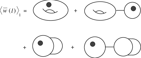
Figure 2: One-loop correlator on the torus.

The reduction formulae do not work for correlation functions involving puncture operator. Instead, one uses the chain rule which follows from eq. (2.19):

$$\langle\bar{P}^{n}\cdots\rangle={\partial^{n}\over\partial\bar{t}^{n}}\,\langle\cdots\rangle=\left({\partial t_{s}\over\partial\bar{t}}\,{\partial\over\partial t_{s}}\right)^{n}=\left(-{1\over\langle PP\rangle_{0}}\,{\partial\over\partial t_{s}}\right)^{n}\ \langle\cdots\rangle\ ,$$ (2.22)

with particular cases

$$\langle\bar{P}\rangle_{0}=\kappa{\partial\over\partial\bar{t}}\,\bar{F}_{0}={\partial\over\partial\bar{t}}\,\Bigl{(}\bar{t}t_{s}+F_{0}(t_{s})\Bigr{)}=t_{s}=\bar{t}^{\,1-\bar{\gamma}}\ ,$$ (2.23)

and

$$\langle\bar{P}\bar{P}\rangle_{0}=-{1\over\langle PP\rangle_{0}}\ .$$ (2.24)

A higher genus example is the one-punctured torus:

$$\langle\bar{P}\rangle_{1}={\partial\over\partial\bar{t}}\,\bar{F}_{1}=-{\langle P\rangle_{1}\over\langle PP\rangle_{0}}+{1\over 2}\,{\langle PPP\rangle_{0}\over\langle PP\rangle_{0}}\ .$$ (2.25)

3 Virasoro Constraints and Recursion Relations

One of the most important mathematical properties of the $c<1$ matrix models is the existence of Virasoro constraints on the partition function (or appropriate generalizations for multi-matrix models). These constraints are equivalent to the loop equations and are related to the integrability property of these models, both on the lattice and in the continuum. When expressed in terms of correlators of local scaling operators, they take the form of recursion relations identical to those defining topological two-dimensional gravity. A nice geometrical picture arises at the multicritical points with $\gamma_{k}=-1/k$: all correlators of scaling operators $\sigma_{m}$ with $m>k-2$ reduce to contact terms at the boundaries of moduli space and can be solved in terms of the correlators of $\sigma_{m}$ with $m<k-1$. This defines the notion of gravitational primaries and descendants, a gravitational version of relevant and irrelevant perturbations of the critical point.

The Virasoro constraints in the continuum take the form  [?,?] (defining $t_{0}\equiv t$):

$$L_{n}Z(t_{0},\{t\})=0\ ,\quad n\geq-1\ ,$$ (3.1)

where $\{t\}=t_{1},t_{2},\dots$, and $Z={\rm e}^{F}$ is the disconnected sum over continuous surfaces. The differential operators $L_{n}$ are given by

$$L_{-1} = \sum_{m\geq 1}\left(m+{1\over 2}\right)t_{m}{\partial\over\partial t_{m-1}}+{t_{0}^{2}\over 8\kappa}\ ,$$

$$L_{0} = \sum_{m\geq 0}\left(m+{1\over 2}\right)t_{m}{\partial\over\partial t_{m}}+{1\over 16}\ ,$$

$$L_{n} = \sum_{m\geq 0}\left(m+{1\over 2}\right)t_{m}{\partial\over\partial t_{m+n}}+{\kappa\over 2}\sum_{m=1}^{n}{\partial^{2}\over\partial t_{m-1}\partial t_{n-m}}\ ,$$ (3.2)

where we made explicit the dependence on $\kappa$, the string loop expansion parameter. These operators satisfy a centerless Virasoro algebra

$$[L_{n},L_{m}]=(n-m)L_{n+m}\ .$$ (3.3)

In the modified matrix models, the partition function (and in general any disconnected correlator) is defined in terms of the corresponding object in the standard matrix model by the Laplace transform

$${\bar{Z}}({\bar{t}_{0}},\{t\})=\int{\rm d}t_{0}\,{\rm e}^{t_{0}{\bar{t}_{0}}/\kappa}Z(t_{0},\{t\})\equiv{\cal L}[Z]\ .$$ (3.4)

This formula makes sense as the saddle point or genus expansion and, as was discussed in the previous section, any correlation function of loops or scaling operators in models of “touching” surfaces may be decomposed into sums of products of correlators of conventional models. It is then clear that the conventional recursion relations imply certain modified recursion relations in the new models, perhaps with a similar topological interpretation. In fact, such relations follow immediately from (3.4) if we define a set of modified Virasoro operators by the operator identity

$$\bar{L}_{n}{\cal L}={\cal L}L_{n}\ ,$$ (3.5)

thus satisfying

$${\bar{L}}_{n}\,{\bar{Z}}({\bar{t}}_{0},\{t\})=0\ ,\quad n\geq-1\ .$$ (3.6)

The new operators are related to those in (3) by the transformations

$$t_{0}\rightarrow\kappa{\partial\over\partial{\bar{t}}_{0}}\ ,\qquad{\partial\over\partial t_{0}}\rightarrow-{\bar{t}_{0}\over\kappa}\ .$$ (3.7)

One can explicitly check that the $\bar{L}_{n}$ operators so defined satisfy the same Virasoro algebra as $L_{n}$. A simple proof of this fact follows from the abstract Fock representation introduced in ref.  [?]. The Virasoro operators (3) can be interpreted in terms of the energy-momentum tensor of a twisted scalar field on the circle, with mode expansion

$$\partial\phi(z)=\sum_{n}\alpha_{n+{1\over 2}}z^{-n-3/2}\ ,$$ (3.8)

under the following substitutions for $n\geq 0$:

$$\alpha_{-n-{1\over 2}}={1\over\sqrt{\kappa}}\left(n+{1\over 2}\right)t_{n}\ ,\qquad\alpha_{n+{1\over 2}}=\sqrt{\kappa}{\partial\over\partial t_{n}}\ .$$ (3.9)

It is easy to see that the Fock space representantion of the modified Virasoro operators is linearly related to the previous one, $\bar{\alpha}_{n+1/2}=\alpha_{n+1/2}$ for $n\neq 0,1$ and $\bar{\alpha}_{1/2}=-2\alpha_{-1/2}$, $\bar{\alpha}_{-1/2}={1\over 2}\alpha_{1/2}$. In fact, it is a Bogoliubov transformation, since it conserves the canonical algebra

$$[\alpha_{n+{1\over 2}},\alpha_{m-{1\over 2}}]=[\bar{\alpha}_{n+{1\over 2}},\bar{\alpha}_{m-{1\over 2}}]=\left(n+{1\over 2}\right)\delta_{n+m,0}$$ (3.10)

from which one derives the Virasoro algebra (3.3) for the $\bar{L}_{n}$ operators.

Recursion relations are easily obtained starting from the general identity:

$$\prod_{j\in S}{\partial\over\partial t_{j}}\left({\rm e}^{-\bar{F}}\,\bar{L}_{n}\,{\rm e}^{\bar{F}}\right)=0\ ,$$ (3.11)

expanded in powers of the string coupling at the $k$th multicritical point, $t_{n}=-\delta_{n,k}/(2k+1)$, $n\geq 1$, with string susceptibility $\bar{\gamma}_{k}=1/(k+1)$. Let us consider for simplicity the case in which there is no puncture operator $\bar{\sigma}_{0}=\bar{P}$ in the set $S$, and use the notation $\bar{\sigma}_{S}\equiv\prod_{S}\bar{\sigma}_{j}$. Neglecting some analytic terms in the couplings, the $L_{-1}$ or puncture equation takes the form:

$$\langle\bar{\sigma}_{k-1}\bar{\sigma}_{S}\rangle_{g}=\sum_{j\in S}(2j+1)\langle\bar{\sigma}_{j-1}\bar{\sigma}_{S-j}\rangle_{g}+{1\over 4}\langle\bar{P}\bar{P}\bar{\sigma}_{S}\rangle_{g-1}+{1\over 8}\sum_{X\cup Y}\sum_{g_{1}+g_{2}=g}\langle\bar{\sigma}_{X}\bar{P}\rangle_{g_{1}}\langle\bar{P}\bar{\sigma}_{Y}\rangle_{g_{2}}\ .$$ (3.12)

The first term on the r.h.s. represents operator contact terms and is identical to the conventional counterpart. However, in the modified model we have additional factorization terms from the contribution of the puncture operator at the boundaries of moduli space, where a genus $g$ surface degenerates into two $g_{1}+g_{2}=g$ surfaces or a $g-1$ surface by pinching a handle.

The $L_{0}$ or dilaton equation is identical to the conventional one, up to a sign flip of the bulk term, proportional to $\bar{t}_{0}$:

$$\langle\bar{\sigma}_{k}\bar{\sigma}_{S}\rangle_{g}=\sum_{j\in S}(2j+1)\langle\bar{\sigma}_{j}\bar{\sigma}_{S-j}\rangle_{g}-\bar{t}_{0}\langle\bar{P}\bar{\sigma}_{S}\rangle_{g}\ .$$ (3.13)

It is interesting that this equation is insensitive to the puncture factorization. The higher $n\geq 1$ equations take the following form:

$$\langle\bar{\sigma}_{k+n}\bar{\sigma}_{S}\rangle_{g} = \sum_{j\in S}(2j+1)\langle\bar{\sigma}_{j+n}\bar{\sigma}_{S-j}\rangle_{g}-2\bar{t}_{0}(1-\delta_{n,1})\langle\bar{\sigma}_{n-1}\bar{\sigma}_{S}\rangle_{g}$$ (3.14)

$$+ \langle\bar{P}\bar{\sigma}_{n}\bar{\sigma}_{S}\rangle_{g-1}+\sum_{m=2}^{n-1}\langle\bar{\sigma}_{m-1}\bar{\sigma}_{n-m}\bar{\sigma}_{S}\rangle_{g-1}$$

$$+ {1\over 2}\sum_{X\cup Y}\sum_{g_{1}+g_{2}=g}\left(\langle\bar{\sigma}_{X}\bar{P}\rangle_{g_{1}}\langle\bar{\sigma}_{n}\bar{\sigma}_{Y}\rangle_{g_{2}}+\sum_{m=2}^{n-1}\langle\bar{\sigma}_{X}\bar{\sigma}_{m-1}\rangle_{g_{1}}\langle\bar{\sigma}_{n-m}\bar{\sigma}_{Y}\rangle_{g_{2}}\right).$$

Again, the operator contact term as well as the factorization terms not involving the puncture operator are identical to the conventional case. The factorization for the puncture is different though: it comes with an extra factor of $1/2$, and the conjugated operator at the degeneration neck is $\bar{\sigma}_{n}$ instead of $\bar{\sigma}_{n-1}$. The bulk term is also slightly different.

These equations are still recursion relations for the gravitational descendants, in the usual sense, and can be derived from the corresponding relations in the conventional models using the diagrammatic method explained in the previous section. This represents a non-trivial check of both the recursion relations and the diagrammatic rules for touching surfaces, due to the complicated pattern of cancellations involved. For this reason it is perhaps surprising that the final result is so similar to the conventional case, with only some modifications in the way the new puncture operator enters in factorization diagrams and bulk terms. We interpret this fact as evidence for an underlying topological field theory description, involving only slight changes from the usual one, perhaps similar to the change of dressing branches, advocated for the Liouville model. Presumably, the rôle of the pure topological point, $k=1$, is played here by the pure polymer phase with $\bar{\gamma}_{1}=1/2$.

To conclude this section, we remark that one can also write integrated forms of the $L_{-1}$ and $L_{0}$ equations acting on loops, measuring boundary lengths and overall dilatations. To this end, we simply insert the loop operator

$$\bar{w}(\ell)={1\over\sqrt{\ell}}{\partial\over\partial\bar{t}_{0}}+\sum_{n\geq 1}{\ell^{n+1/2}\over\Gamma(n+3/2)}{\partial\over\partial t_{n}}$$ (3.15)

on the left hand side of eq. (3.11).

We find some differences with respect to the conventional models. The dilaton operator, which at the $k$th critical point is $\bar{\sigma}_{k}$, satisfies

$${1\over 2}\langle\bar{\sigma}_{k}\bar{w}(\ell)\rangle=\left(-{1\over 2}\bar{t}_{0}{\partial\over\partial\bar{t}_{0}}+\ell{\partial\over\partial\ell}\right)\langle\bar{w}(\ell)\rangle\ .$$ (3.16)

Comparing with the conventional models, the sign of the bulk term is flipped. In the modified models we find additional non-local terms associated with the new puncture contributions to the $L_{-1}$ constraint, as well as an inhomogeneus term, proportional to the one-puncture function,

$${1\over 2}\langle\bar{\sigma}_{k-1}\bar{w}(\ell)\rangle=\ell\langle\bar{w}(\ell)\rangle-\sqrt{\ell}\langle\bar{P}\rangle+{1\over 8}\left(\kappa\langle\bar{P}\bar{P}\bar{w}(\ell)\rangle+2\langle\bar{P}\rangle\langle\bar{P}\bar{w}(\ell)\rangle\right)\ ,$$ (3.17)

where we have neglected some analytic terms. Thus, it seems that a local boundary operator is absent in the modified models. ($\sigma_{k-1}$ acts as a boundary operator in the conventional models due to the relation ${1\over 2}\langle\sigma_{k-1}w(\ell)\rangle=\ell\langle w(\ell)\rangle$.) There are interesting generalizations of the above exercise. For example, one may consider $W$-constraints for modified multi-matrix models. Also, other operators can be tuned as wormhole sources. In the most general case one has a multiple Laplace transform and still a Bogoliubov transformation in the Fock space representation.

4 Changing Gravitational Dimensions

In the previous sections we studied modified one-matrix models with the simplest type of trace squared term, $({\rm Tr\,}\Phi^{4})^{2}$. We showed that the effect of this term is to change the branch of gravitational dressing of the lowest dimension operator in the theory, which corresponds to coupling constant $t$. In this section we check that more complicated trace-squared terms alter the gravitational dimensions of other scaling operators. In particular, we check in detail that formula (1.7), first derived in ref.  [?], applies to gravitational descendants.

Although our approach is general, we focus for simplicity on the $k=2$ one-matrix model, whose matrix potential is

$$S_{0}(\Phi)=N{\rm Tr\,}({1\over 2}\Phi^{2}-\lambda\Phi^{4})\ .$$ (4.1)

The continuum limit is achieved as $\Delta=\lambda_{c}-\lambda\rightarrow 0$. It is convenient to introduce the first scaling operator of the form

$$\sigma_{1}=N{\rm Tr\,}\left(\Phi^{2}-{1\over 12}\Phi^{4}\right)-N^{2}(1-16\Delta-2304\Delta^{2})\ .$$ (4.2)

This operator has gravitational dimension $d=1/2$, and its connected genus zero correlation functions are given by

$$\langle\sigma_{1}\rangle=N^{2}{\cal O}(\Delta^{5/2})\ ,$$

$$\langle\sigma_{1}\sigma_{1}\rangle=N^{2}({4\over 3}-1024\sqrt{3}\Delta^{3/2}+{\cal O}(\Delta^{2}))\ ,$$

$$\langle\sigma_{1}\sigma_{1}\sigma_{1}\rangle=N^{2}(1536\Delta+{\cal O}(\Delta^{3/2}))\ ,$$

$$\langle\sigma_{1}\sigma_{1}\sigma_{1}\sigma_{1}\rangle=N^{2}(-768\sqrt{3}\Delta^{1/2}+{\cal O}(\Delta))\ ,\ {\rm etc.}$$ (4.3)

The purpose of the $\Phi$-independent term in $\sigma_{1}$ is to remove a non-universal analytic term from the one-point function. Apart from this it has no effect.

Now we consider a modified model with the action

$$S_{0}(\Phi)-\tau_{1}\sigma_{1}-{g\over 2N^{2}}(\sigma_{1})^{2}\ ,$$ (4.4)

where we have introduced coupling constant $\tau_{1}$ in order to study correlation functions of $\sigma_{1}$. Its partition function may be written as

$$Z\sim\int_{-\infty}^{\infty}{\rm d}v\,{\rm e}^{-{N^{2}v^{2}\over 2g}}\int{\cal D}\Phi\,{\rm e}^{-S_{0}+(v+\tau_{1})\sigma_{1}}\ .$$ (4.5)

Defining a shifted variable $u=v+\tau_{1}$, we perform the matrix integral first and reduce the modified free energy to

$$\bar{F}=F_{0}(t)+\log\int{\rm d}u\,{\rm e}^{f(u)}\ ,$$

$$f(u)=-{N^{2}\over 2g}(u^{2}-2u\tau_{1}+\tau_{1}^{2})+{4\over 3}N^{2}u^{2}+F_{1}(t,t_{1})\ ,$$ (4.6)

where the scaling variables $t$ and $t_{1}$ are defined through

$$t\sim\Delta N^{2/(2-\gamma)}\ ,\qquad\qquad t_{1}=uN^{2(1-d)/(2-\gamma)}\ .$$ (4.7)

In this specific case $\gamma=-1/2$ and $d=1/2$. Of crucial importance is the fact the $F_{1}$ depends only on the scaling variables and has the form

$$F_{1}(t,t_{1})=\sum_{n=2}^{\infty}a_{n}t_{1}^{n}t^{(5-n)/2}\ ,$$ (4.8)

where $a_{n}$ are constants (the first three of them may be read off eq. (4)). This follows from miraculous vanishing of certain potentially harmful non-universal terms in eq. (4). For example, had the three-point function of $\sigma_{1}$ started with a non-universal term of order $\Delta^{0}$, eq. (4.8) would not be valid!

If we now set $g=3/8$ and introduce the scaling variable

$$\bar{t}_{1}={8\over 3}\tau_{1}N^{2(1-\bar{d})/(2-\gamma)}\ ,$$ (4.9)

we arrive at the following expression for the universal part of the modified free energy,

$$\bar{F}(t,\bar{t}_{1})=\log\int_{-\infty}^{\infty}{\rm d}t_{1}\,{\rm e}^{t_{1}\bar{t}_{1}+F(t,t_{1})}\ ,$$ (4.10)

Here $F(t,t_{1})$ is the universal part of the conventional sum over surfaces. Thus, we find that the gravitational dimension of $\sigma_{1}$ has changed from $d=1/2$ to $\bar{d}=\gamma-d=-1$. This provides a counterexample to the claim of ref.  [?] that eq. (1.7) applies only to operators with $d\leq(1+\gamma)/3$.

While in ref.  [?] eq. (1.7) was derived for gravitational primary fields, we have just checked it for a gravitational descendant. Our example shows that these operators have to be defined in such a way that their correlation functions do not contain certain non-universal contributions. We believe that this is in fact always possible. As further evidence, we present results for the dilaton operator,

$$\sigma_{2}=N{\rm Tr\,}\left(2\Phi^{2}-{1\over 3}\Phi^{4}+{1\over 60}\Phi^{6}\right)-N^{2}\left({8\over 5}-{64\over 5}\Delta\right).$$ (4.11)

This operator has gravitational dimension $d=1$, and its connected genus zero correlation functions are given by

$$\langle\sigma_{2}\rangle\sim N^{2}\Delta^{5/2}\ ,$$

$$\langle\sigma_{2}\sigma_{2}\rangle=N^{2}({32\over 15}+{\cal O}(\Delta^{5/2}))\ ,$$

$$\langle\sigma_{2}\sigma_{2}\sigma_{2}\rangle\sim N^{2}\Delta^{5/2}\ ,$$

$$\langle\sigma_{2}\sigma_{2}\sigma_{2}\sigma_{2}\rangle\sim N^{2}\Delta^{5/2}\ ,\ {\rm etc.}$$ (4.12)

Once again, the unwanted non-universal terms vanish! Repeating the steps carried out for $\sigma_{1}$, we may now establish the validity of (1.7) for $\sigma_{2}$. This relation, and the change of gravitational dimension it implies, appear to be completely general.

5 Correlators of Dressed Primary Fields

In the previous section we studied correlation functions of gravitational descendants in modified one-matrix models. In this section we turn to gravitationally dressed primary fields. Although our approach is general, we mostly discuss some simple special cases: genus zero two- and three-point functions of the order parameter fields in unitary minimal models coupled to gravity, as well as the four-point function for $c=1$. We find that the correlators in modified matrix models agree with those of negatively dressed operators in Liouville theory, provided that the latter are obtained with the simplest plausible analytic continuation prescription. Although a far better understanding of the Liouville theory calculations is desirable, we feel that our findings suggest a general pattern for interpreting the modified matrix models in terms of the negatively dressed operators.

The starting point for our calculations is the relation (1.7) between the genus zero free energy $\bar{F}$ of the modified matrix model and that of the original matrix model, $F$:

$$\bar{F}(\bar{t}_{1},\bar{t}_{2},...)=\sum_{i}t_{i}\bar{t}_{i}+F(t_{1},t_{2},...),\qquad\qquad{\partial F\over\partial t_{j}}=-\bar{t}_{j}\ ,$$ (5.1)

where $t_{i}$ and $\bar{t}_{i}$ represent the coupling constants by which the model is perturbed (it is implicit that $F$ and $\bar{F}$ also depend on the basic coupling constant $t$, which appears in the Liouville action). Since $t_{i}$ correspond to dressed primary fields, $F$ has the expansion

$$F(t_{i})={1\over 2}\Delta_{i}t_{i}^{2}+{1\over 6}c_{ijk}t^{i}t^{j}t^{k}+{1\over 24}d_{ijkl}t^{i}t^{j}t^{k}t^{l}+\dots$$ (5.2)

where $\Delta_{i},c_{ijk},d_{ijkl}$ are the ordinary two-, three- and four-point functions. $\bar{F}$ in (5.1) can be evaluated order by order in the $\bar{t}_{i}$ by expanding $t_{i}\bar{t}_{i}+F(t_{i})$ around the saddle point.

Let us begin by discussing the two- and three-point functions. First assume that there is only one parameter $t_{i}$. Then the Legendre transform fixes $t_{i}$ at

$$t_{i0}=-{1\over\Delta_{i}}\bar{t}_{i}-{c_{iii}\over 2\Delta_{i}^{3}}\bar{t}_{i}^{\,2}+\dots$$ (5.3)

The genus zero part of $\bar{F}$ is just the value of $t_{i}\bar{t}_{i}+F(t_{i})$ at $t_{i0}$. One finds in this case

$$\bar{F}(\bar{t}_{i})={1\over 2}\Delta_{\bar{\imath}}\bar{t}_{i}^{\,2}+{1\over 6}c_{\bar{\imath}\bar{\imath}\bar{\imath}}\bar{t}_{i}^{\,3}+\dots$$ (5.4)

with modified two- and three-point functions

$$\Delta_{\bar{\imath}}=-{1\over\Delta_{i}}\ ,\qquad c_{\bar{\imath}\bar{\imath}\bar{\imath}}=-{c_{iii}\over\Delta_{i}^{3}}\ .$$ (5.5)

Next, assume that there are two parameters $t_{i},t_{k}$ and one wants to modify one of them, i.e., one wants to find $\bar{F}(\bar{t}_{i},t_{k})$ to cubic order. Now the saddle point is at

$$t_{i0}=\left(-{1\over\Delta_{i}}+{c_{iik}\over 3\Delta_{i}^{2}}t_{k}\right)\bar{t}_{i}+\dots$$ (5.6)

In this case,

$$\bar{F}(\bar{t}_{i},t_{k})={1\over 2}\Delta_{\bar{\imath}}\bar{t}_{i}^{\,2}+{1\over 2}\Delta_{k}t_{k}^{2}+{1\over 6}c_{\bar{\imath}\bar{\imath}k}\bar{t}^{i}\bar{t}^{i}t^{k}+{1\over 6}c_{\bar{\imath}kk}\bar{t}^{i}t^{k}t^{k}+\dots$$ (5.7)

with

$$\Delta_{\bar{\imath}}=-{1\over\Delta_{i}}\ ,\qquad c_{\bar{\imath}\bar{\imath}k}=+{c_{iik}\over\Delta_{i}^{2}}\ ,\qquad c_{\bar{\imath}kk}=-{c_{ikk}\over\Delta_{i}}\ .$$ (5.8)

The generalization is straightforward: each time we Legendre transform from $t_{i}$ to $\bar{t}_{i}$ the two- and three-point functions change according to

$$\Delta_{i}\rightarrow\Delta_{\bar{\imath}}=-{1\over\Delta_{i}}\ ,\qquad c_{ijk}\rightarrow c_{\bar{\imath}jk}=-{c_{ijk}\over\Delta_{i}}\ .$$ (5.9)

The absolute values of the correlators are normalization dependent, so it is useful to define the normalization independent quantity as in ref.  [?]:

$$X_{ijk}={c_{ijk}^{2}\over\Delta_{i}\Delta_{j}\Delta_{k}}F\ ,$$ (5.10)

where $F$ is the free energy evaluated at $t_{i}=0$. One easily sees from eq. (5.9) that $X$ has a simple property: it just switches sign each time one of the external operators is modified, i.e.

$$X_{\bar{\imath}jk}=-X_{ijk}\ ,\qquad X_{\bar{\imath}\bar{\jmath}k}=X_{ijk}\ ,\qquad X_{\bar{\imath}\bar{\jmath}\bar{k}}=-X_{ijk}\ .$$ (5.11)

Let us compare this behavior with what one would expect from Liouville theory, if the modified matrix model operators $\bar{\cal O}_{i}$ were identified with the negatively dressed operators. Consider the $q$th minimal model with central charge

$$c=1-{6\over q(q+1)}\ ,$$

coupled to gravity. The gravitationally dressed operators on the diagonal of the Kac table are

$${\cal O}_{i}=\psi_{r_{i},r_{i}}\,{\rm e}^{\beta_{i}^{+}\phi}\ ,\qquad\qquad\bar{\cal O}_{i}=\psi_{r_{i},r_{i}}\,{\rm e}^{\beta_{i}^{-}\phi}\ ,$$ (5.12)

with

$$\beta_{i}^{\pm}=-{Q\over 2}\pm\omega_{i}\ ,\qquad\omega_{i}={r_{i}\over{\sqrt{2q(q+1)}}}\ .$$

We note that switching from the $\beta_{i}^{+}$ to the $\beta_{i}^{-}$ dressing corresponds to continuing $r_{i}\rightarrow-r_{i}$. The dressed unity $e^{\alpha_{+}\phi}$ corresponds to the puncture operator with $r_{i}=1$. As shown in section 2, if we Legendre transform with respect to the cosmological constant $t$, as in eq. (2.10), we find a new theory with Liouville potential $e^{\alpha_{-}\phi}$.

First, note that the scaling behavior of the modified correlators (5.5) and (5.8) is that of operators with the $\beta^{-}_{i}$ dressing. This has already been noted in ref.  [?] and in section 4. Next, let us compare the coefficients. Consider the quantities $X_{ijk}$, defined in (5.10). They can be derived from the fact that the three-point function of the properly normalized operators can be written as  [?]

$$\langle{\cal O}_{i}{\cal O}_{j}{\cal O}_{k}\rangle=t^{-{Q\over\alpha_{+}}-{\beta_{i}^{+}+\beta_{j}^{+}+\beta_{k}^{+}\over\alpha_{+}}}\ .$$ (5.13)

Since insertions of the puncture operator $P$ are produced by $-\partial_{t}$, we can infer from (5.13) and from the scaling behavior the two-point function and the partition function:

$$-\partial_{t}\langle{\cal O}_{k}{\cal O}_{k}\rangle=\langle P{\cal O}_{k}{\cal O}_{k}\rangle=t^{-{Q\over\alpha_{+}}-2{\beta_{k}^{+}\over\alpha_{+}}-1}\ \ \Rightarrow\ \ \langle{\cal O}_{k}{\cal O}_{k}\rangle={\alpha_{+}\over Q+2\beta_{k}^{+}}\,t^{-{Q\over\alpha_{+}}-2{\beta_{k}^{+}\over\alpha_{+}}}\ ,$$ (5.14)

and

$$\partial_{t}^{2}F=\langle PP\rangle={\alpha_{+}\over Q+2\alpha_{+}}t^{-{Q\over\alpha_{+}}-2}\ \ \Rightarrow\ \ F={1\over{Q\over\alpha_{+}}({Q\over\alpha_{+}}+1)({Q\over\alpha_{+}}+2)}\,t^{-{Q\over\alpha_{+}}}\ .$$ (5.15)

We thus obtain

$$X_{ijk}={\langle{\cal O}_{i}{\cal O}_{j}{\cal O}_{k}\rangle^{2}F\over\langle{\cal O}_{i}{\cal O}_{i}\rangle\langle{\cal O}_{j}{\cal O}_{j}\rangle\langle{\cal O}_{k}{\cal O}_{k}\rangle}={(Q+2\beta_{i}^{+})(Q+2\beta_{j}^{+})(Q+2\beta_{k}^{+})\over Q(Q+\alpha_{+})(Q+2\alpha_{+})}\sim r_{i}r_{j}r_{k}\ .$$ (5.16)

This is the result of Goulian and Li  [?]. In order to calculate $X_{\bar{\imath}jk}$ we assume that it is given by the above equation with $\beta^{+}$ replaced by $\beta^{-}$. This procedure is consistent with all the tricks used in the Liouville theory calculations  [?]. The result is remarkably simple: $X_{\bar{\imath}jk}=-X_{ijk}$, in agreement with (5.11). In general, $X_{ijk}$ simply switches sign each time one of the Liouville dressings is modified from $\beta^{+}$ to $\beta^{-}$. It appears that we have found an explanation for the changes of sign caused by Legendre transform (5.1). Remarkably, they have the same effect on correlation functions as changes in the sign of the Liouville energies.

Equally remarkable is the effect on (5.16) of Legendre transforming with respect to the cosmological constant $t$ only, as in eq. (2.10). In this modified matrix model we find

$$\bar{F}={1\over{Q\over\alpha_{+}}({Q\over\alpha_{+}}+2)}\,(C\bar{t}\,)^{-{Q\over\alpha_{-}}}\ ,$$ (5.17)

where $C=({Q\over\alpha_{+}}+1)({Q\over\alpha_{+}}+2)$. Correlation functions of order parameters other than the puncture become “one-puncture irreducible” and may be computed using the same rules as in eqs. (2.12)–(2). The modifications are trivial because one-point functions vanish, and we arrive at

$$\langle{\cal O}_{k}{\cal O}_{k}\rangle={\alpha_{+}\over Q+2\beta_{k}^{+}}\,(C\bar{t}\,)^{-{Q\over\alpha_{-}}-2{\beta_{k}^{+}\over\alpha_{-}}}\ ,$$

$$\langle{\cal O}_{i}{\cal O}_{j}{\cal O}_{k}\rangle=(C\bar{t}\,)^{-{Q\over\alpha_{-}}-{\beta_{i}^{+}+\beta_{j}^{+}+\beta_{k}^{+}\over\alpha_{-}}}\ .$$ (5.18)

This leads to

$$\bar{X}_{ijk} = {\langle{\cal O}_{i}{\cal O}_{j}{\cal O}_{k}\rangle^{2}\bar{F}\over\langle{\cal O}_{i}{\cal O}_{i}\rangle\langle{\cal O}_{j}{\cal O}_{j}\rangle\langle{\cal O}_{k}{\cal O}_{k}\rangle}={(Q+2\beta_{i}^{+})(Q+2\beta_{j}^{+})(Q+2\beta_{k}^{+})\over Q\alpha_{+}(Q+2\alpha_{+})}$$ (5.19)

$$= {(Q+2\beta_{i}^{+})(Q+2\beta_{j}^{+})(Q+2\beta_{k}^{+})\over Q(Q+\alpha_{-})(Q+2\alpha_{-})}\ .$$

Thus, the sole effect of the Legendre transform with respect to $t$ is to replace $\alpha_{+}$ by $\alpha_{-}$ in eq. (5.16)! This precisely agrees with the idea that the dressing of the Liouville potential has changed from $e^{\alpha_{+}\phi}$ to $e^{\alpha_{-}\phi}$.

To generalize our observations to the four-point function, it is useful to note that the relation between $F(t_{i})$ and $\bar{F}(\bar{t}_{i})$ is the same as that between $W(j)$, the generating function of the connected diagrams, and $S(\phi)$, the effective action,

$${\rm e}^{S(\phi)}=\int{\rm d}j\ {\rm e}^{j\phi+W(j)}\ .$$ (5.20)

At tree level $S(\phi)$ is identical to the generating function $\Gamma(\phi)$ of one-particle irreducible diagrams. Based on this analogy, we can graphically represent the relation between modified correlators (black circles) and original correlators (white circles) in terms of Feynman diagrams. Let us illustrate this with some examples:

One indeed recognizes formulae (5.5) in the first two lines (A), (B). Example (C) refers to the four-point function Legendre transformed only with respect to a coupling corresponding to an operator appearing in the intermediate state (the couplings corresponding to external legs remain untouched). This changes the value of the four-point function according to

$$d_{ijkl}\rightarrow d_{ijkl}-c_{ijm}{1\over\Delta_{m}}c_{mkl}.$$ (5.21)

The implications of this are quite significant. In the language of Liouville theory, we have not modified the action, nor have we modified any of the operators entering the four-point function. Nevertheless, the value of the correlator changed. A similar effect was observed in  [?] in the course of calculating the genus one free enegy: it changed in response to changing the dressing of any operator, even though the Liouville action remained untouched. This suggests a remarkable subtlety in the continuum Liouville calculations, related perhaps to contributions from boundaries of moduli spaces.

In figure (D) we show a simpler example where a four-point function is Legendre transformed only with respect to a coupling corresponding to an external state, so that

$$d_{\bar{\imath}jkl}=-{1\over\Delta_{i}}d_{ijkl}\ .$$ (5.22)

Finally, in example (E) we demonstrate the most general transformation of the four-point function under the Legendre transform of some set of coupling constants,

$$d_{\bar{\imath}\bar{\jmath}\bar{k}\bar{l}}={d_{ijkl}\over\Delta_{i}\Delta_{j}\Delta_{k}\Delta_{l}}-\left\{\sum_{m}{1\over\Delta_{i}}{1\over\Delta_{j}}c_{ijm}{1\over\Delta_{m}}c_{mkl}{1\over\Delta_{k}}{1\over\Delta_{l}}+\hbox{crossing terms}\right\}.$$ (5.23)

The sum over $m$ runs over all intermediate operators whose coupling constants are Legendre transformed.

The above discussion suggests that it is useful to introduce the normalization independent quantity

$$X_{ijkl}={1\over\Delta_{i}\Delta_{j}\Delta_{k}\Delta_{l}}\left\{d_{ijkl}-{1\over 2}\left(\sum_{m}c_{ijm}{1\over\Delta_{m}}c_{mkl}+\hbox{crossing terms}\right)\right\}^{2}\ F\ .$$ (5.24)

(Note the factor $1/2$ in comparing with (5.23) and (5.21).) Here, the sum over $m$ runs over all operators. Using (5.9), (5.21) and (5.22) we establish that $X$ is invariant under the Legendre transform with respect to any intermediate operator, but switches sign each time an external operator is transformed.

Let us compare this with the behavior of correlation functions in $c=1$ theory coupled to gravity. We introduce positively and negatively dressed tachyon operators,

$$V_{q}={\Gamma(1+|q|)\over\Gamma(1-|q|)}\int{\rm d}^{2}\sigma\,{\rm e}^{iqX+(-2+|q|)\phi}\ ,\qquad\bar{V}_{q}={\Gamma(1-|q|)\over\Gamma(1+|q|)}\int{\rm d}^{2}\sigma\,{\rm e}^{iqX+(-2-|q|)\phi}\ ,$$ (5.25)

normalized to remove the usual external leg factors from the correlation functions. For the two-, three-, and four-point functions of positively dressed operators in the conventional Liouville theory we have  [?]

$$\Delta_{q_{i}}=-{1\over|q_{i}|}t^{|q_{i}|}\ ,\qquad c_{q_{1}q_{2}q_{3}}=\delta(\sum_{i}q_{i})t^{-1+(|q_{1}|+|q_{2}|+|q_{3}|)/2}\ ,$$

$$d_{q_{1}q_{2}q_{3}q_{4}}=\delta(\sum_{i}q_{i})t^{-2+(|q_{1}|+|q_{2}|+|q_{3}|+|q_{4}|)/2}\left(1-{|q_{1}+q_{2}|\over 2}-{|q_{1}+q_{3}|\over 2}-{|q_{1}+q_{4}|\over 2}\right).~{}~{}~{}$$ (5.26)

We may now modify the theory as in example (C), by changing the dressing of the operator with momentum $q_{1}+q_{2}$. We assume that this flips the sign of the Liouville energy corresponding to this state appearing in the intermediate channel, and the resulting four-point function is

$$d_{q_{1}q_{2}q_{3}q_{4}}=\delta(\sum_{i}q_{i})t^{-2+(|q_{1}|+|q_{2}|+|q_{3}|+|q_{4}|)/2}\left(1+{|q_{1}+q_{2}|\over 2}-{|q_{1}+q_{3}|\over 2}-{|q_{1}+q_{4}|\over 2}\right)\ .$$ (5.27)

Similarly, the change of dressing of the $q_{1}+q_{3}$ operator changes the sign of the corresponding term in the four-point function, etc. It is easy to check, though, that the quantity $X_{ijkl}$, defined in (5.24), is invariant under these changes. In fact,

$$X_{q_{1}q_{2}q_{3}q_{4}}=|q_{1}||q_{2}||q_{3}||q_{4}|\ .$$ (5.28)

A change of dressing of one of the external operators is implemented by $|q_{i}|\rightarrow-|q_{i}|$, which indeed flips the sign of $X$. These properties of $X_{q_{1}q_{2}q_{3}q_{4}}$, found with plausible assumptions about Liouville theory, are in complete agreement with our calculations in modified matrix model. All other normalization independent quantities involving three- and four-point functions can be built from (5.10) and (5.24). The correlators of modified operators thus agree with the correlators of negatively dressed operators, up to possible rescalings of the operators. We expect that this agreement extends to higher-point functions.

It is interesting that behind the four-point function, which is quite complex, we have uncovered a more fundamental object, $X_{q_{1}q_{2}q_{3}q_{4}}$, which transforms very simply under changes of the Liouville dressing. It would be interesting to check if such simpler objects can be defined for higher-point functions. Construction of such objects is reminiscent of the work of Di Francesco and Kutasov  [?] who built the $c=1$ correlators in terms of more elementary “vertices”. Perhaps such objects hold the key to a better understanding of the Liouville calculations.

6 Conclusion

The recently improved understanding of the modified matrix models with fine-tuned wormhole weights opens the possibility of many new insights into random surfaces. In this paper we have calculated some of the simplest modified correlation functions, and there are many possible generalizations of our work. It is remarkable that our calculations, which on a sphere reduce to Legendre transforms, have a hidden relation to operators with the negative branch of Liouville dressing. We hope that more progress will come from a deeper understanding of this effect.

Appendix A ppendix A

In this appendix we give a careful derivation of the fundamental formula relating the continuum one-matrix models and corresponding modified models:

$${\rm e}^{\bar{F}(\bar{t},\{t\})}=\int{\rm d}t\,\,{\rm e}^{t\bar{t}+F(t,\{t\})}$$ (A.1)

where $\{t\}=\{t_{1},t_{2},\dots\}$ are couplings to scaling operators around a particular critical point. Apparently the scaling operators $\sigma_{n}$ conjugate to $t_{n}$, $n\geq 1$ are spectators in the continuum formula (A.1), so that we can extend it to any correlator without punctures

$$\langle\bar{\sigma}_{i_{1}}\dots\bar{\sigma}_{i_{s}}\rangle_{\rm disconn.}=\int{\rm d}t\,\,{\rm e}^{t\bar{t}}\langle\sigma_{i_{1}}\dots\sigma_{i_{s}}\rangle_{\rm disconn.}\ .$$ (A.2)

However, it turns out that the matrix model proof of (A.1) involves some subtleties, due to the fact that the $discrete$ scaling operators in the old and the modified models are not exactly the same.

Let us consider a perturbation of the $k$th multicritical modified matrix model of the form (we use even potentials for simplicity):

$$Z_{k}[\lambda,g,\{\bar{\tau}\}]=\int\,{\cal D}\Phi\,{\rm e}^{-N\left({\rm Tr\,}V_{k}(\Phi)+(c_{2}-\lambda){\rm Tr\,}\Phi^{4}-{g\over 2N}({\rm Tr\,}\Phi^{4})^{2}+\sum_{n\geq 1}\bar{\tau}_{n}\bar{\sigma}_{n}\right)}.$$ (A.3)

The multicritical potential is identical to the one of the conventional model,

$$V_{k}(\Phi)=\sum_{p\geq 1}c_{p}\,\Phi^{2p}\ ,$$ (A.4)

and $\lambda$ is the bare cosmological constant. The bare scaling operators have the general form

$$\bar{\sigma}_{n}=\sum_{p\geq 1}\bar{g}_{p}^{(n)}{\rm Tr\,}\Phi^{2p}\ .$$ (A.5)

The coefficients $\bar{g}_{p}^{(n)}$ can be explicitly computed in this model, because the planar limit is solvable. Let us review the main points involved in the solution (see ref.  [?]).

All planar properties can be extracted from the eigenvalue density. In the one-cut phase it is given by

$$\rho(x)={1\over 2\pi}\sum_{m,k\geq 0}(m+k+1)A_{k}(R){\tilde{g}}_{m+k+1}x^{m}\sqrt{R-x^{2}}\ ,$$ (A.6)

with the definitions

$${\tilde{g}}_{p}=c_{p}+\bar{\tau}\cdot\bar{g}_{p}-g\Bigl{\langle}{1\over N}\,{\rm Tr\,}\Phi^{4}\Bigr{\rangle}\,\delta_{p,2}\ ,$$ (A.7)

$$A_{k}(R)={2k\choose k}\left({R\over 4}\right)^{k}\ .$$ (A.8)

Since $\tilde{g}_{p}$ depends on the ${\rm Tr\,}\Phi^{4}$ condensate we are led to a self-consistent problem given by the equation

$$\Bigl{\langle}{1\over N}\,{\rm Tr\,}\Phi^{4}\Bigr{\rangle}=\int{\rm d}x\,\rho(x)\,x^{4}\ .$$ (A.9)

Fortunately, for the model at hand the condensate enters only linearly in this equation, and we can solve explicitly for the feedback. The final answer for the cosmological constant as a function of the eigenvalue endpoint is

$$\lambda(R)=-{1\over 2A_{2}^{2}}\left(1+gA_{2}^{2}-\sum_{p\geq 1}pA_{p}\left(1-{p-2\over p+2}gA_{2}^{2}\right)(c_{p}-c_{2}+\bar{\tau}\cdot\bar{g}_{p})\right)\ .$$ (A.10)

Also, the string susceptibility is given by

$$\chi={{\rm d}\over{\rm d}\lambda}\Bigl{\langle}{1\over N}\,{\rm Tr\,}\Phi^{4}\Bigr{\rangle}={A_{2}^{2}\over 1-gA_{2}^{2}}\ .$$ (A.11)

For $\bar{\tau}=0$ a critical point with positive susceptibility exponent $\bar{\gamma}_{k}={1\over k+1}$ occurs at $R_{c}$ when

$$\chi\sim(R-R_{c})^{-1}\qquad{\rm and}\qquad\lambda(R)\sim\lambda(R_{c})+C(R-R_{c})^{k+1}\ .$$ (A.12)

If we set $R_{c}=8$, then the critical value of $g$ is $g_{c}=1/576$. Scaling operators are defined as deformations of eq. (A.12) which do not shift the location of the critical point $g_{c}$ and $\lambda(R_{c})$. This is an important requirement because, in the end we want the couplings $\bar{\tau}$ to act as sources, and non-universal dependence on $\bar{\tau}$ through the value of the critical point invalidates the scaling property. As a result, scaling operators (already in conventional matrix models) involve one more tuning than the multicritical potentials.

From eq. (A.10) we find the critical conditions for the coefficients of $\bar{\sigma}_{n}$, $n\geq 1$:

$$\lambda_{n}(R)={1\over 2A_{2}^{2}}\sum_{p\geq 1}pA_{p}\left(1-{p-2\over p+2}gA_{2}^{2}\right)\bar{g}_{p}^{(n)}\,\,\sim\,\,(R-8)^{n+\alpha}\ ,$$ (A.13)

where $\alpha$ is a positive integer. In the conventional models $g=0$ and $\alpha=0$. Remarkably, $\alpha=1$ in the modified models. Indeed, the derivative of (A.13) is

$${{\rm d}\lambda_{n}\over{\rm d}R}=-{1-gA_{2}^{2}\over 2A_{2}R}\sum_{p\geq 1}p(p-2)A_{p}\bar{g}_{p}^{(n)}\sim(R-8)^{n+\alpha-1}\ .$$ (A.14)

At the critical points with positive $\bar{\gamma}$ we have $g=1/576$, $1-gA_{2}^{2}\sim R-8$ and $\lambda_{n}(R)$ is at least quadratic in $R-8$ for $n\geq 1$. This shift is ultimately responsible for the absence of a scaling operator with dimension $\bar{\gamma}_{k}$. From (A.14) we also see that the scaling operators in the modified model differ from those at $g=0$ only in the coefficient of ${\rm Tr\,}\Phi^{4}$ which does not enter (A.14), and is determined from (A.13) by requiring stability of the critical point. The final result is

$$\bar{\sigma}_{n}=\sigma_{n}+\delta g_{2}^{(n)}\,{\rm Tr\,}\Phi^{4}\ ,$$ (A.15)

where $\sigma_{n}$ is the conventional bare scaling operator, and

$$\delta g_{2}^{(n)}={1\over 48}\sum_{p}{p(p-2)\over p+2}{2p\choose p}2^{p}\bar{g}_{p}^{(n)}\ ,$$ (A.16)

with a spectrum of gravitational dimensions at the $k$th critical point:

$$d(\bar{\sigma}_{n})=(n+1)\bar{\gamma}_{k}={n+1\over k+1}\ .$$ (A.17)

We see that the bare operators in the two phases are different by a shift of the ${\rm Tr\,}\Phi^{4}$ term. Alternatively, we can work with the same deformations and a shifted cosmological constant $\lambda\rightarrow\lambda+\bar{\tau}\cdot\delta g_{2}$. It turns out that the required redefinition of $\lambda$ ensures the delicate balance of non-universal terms needed for the scaling of formula (A.1).

Setting $\bar{\tau}_{n}=\tau_{n}$ we write

$$\bar{\tau}\cdot\bar{\sigma}=\tau\cdot\sigma+\tau\cdot\delta g_{2}{\rm Tr\,}\Phi^{4}$$ (A.18)

and, following ref.  [?] we introduce the Gaussian representation

$$Z_{k}[g,\lambda,\{\tau\}]={N\over\sqrt{2\pi g}}\int_{-\infty}^{+\infty}{\rm d}x\,{\rm e}^{-{N^{2}\over 2g}(\lambda+\tau\cdot\delta g_{2}-c_{2}-x)^{2}}Z_{k}[g=0,c_{2}-x,\{\tau\}]\ .$$ (A.19)

Note that $Z_{k}$ in the integrand is the partition function of the $k$-th multicritical model, deformed by the conventional scaling operators. Next we separate the non-universal (analytic in $x$) terms on the sphere

$${\rm log}Z_{k}[g=0,c_{2}-x,\{\tau\}]=N^{2}\left(-a_{1}^{\{\tau\}}\,x+{1\over 2}a_{2}^{\{\tau\}}\,x^{2}\right)+F(x,\{\tau\},N^{2})\ .$$ (A.20)

The $\tau$ dependence of the coefficients $a_{1},a_{2}$ can be extracted from the previously studied planar solution

$$a_{2}^{\{\tau\}}={{\rm d}\over{\rm d}\lambda}\Bigl{\langle}{1\over N}\,{\rm Tr\,}\Phi^{4}\Bigr{\rangle}(g=0,\lambda=c_{2})={4\choose 2}^{2}\left({R_{c}\over 4}\right)^{2}=576\ .$$ (A.21)

Note that $a_{2}=576$ independently of $\tau_{n}$. On the other hand, $a_{1}$ depends linearly on $\tau$:

$$a_{1}^{\{\tau\}}=\Bigl{\langle}{1\over N}{\rm Tr\,}\Phi^{4}\Bigr{\rangle}(g=0,\lambda=c_{2})=a_{1}(\tau=0)+576\,\tau\cdot\delta g_{2}=a_{1}+a_{2}\,\tau\cdot\delta g_{2}\ .$$ (A.22)

Finally, we can write the Laplace transform, ready for scaling

$$Z_{k}[g,\lambda,\{\tau\}]={\rm const.}\times\int_{-\infty}^{+\infty}{\rm d}x\,e^{N^{2}a_{2}x\Delta+F(x,\{\tau\},N^{2})}\ ,$$ (A.23)

where $\Delta$ is given by

$$\Delta=\lambda-\lambda_{c}=\lambda-c_{2}+\tau\cdot\delta g_{2}-{a_{1}^{\{\tau\}}\over a_{2}}=\lambda-c_{2}-{a_{1}\over a_{2}}\ ,$$ (A.24)

and the scaling variable $\Delta$ is independent of the scaling deformations $\tau_{n}$. As a result, we can safely take derivatives in $\tau_{n}$ to obtain a discrete version of (A.2). We see that the slight difference between $\bar{\sigma}_{n}$ and $\sigma_{n}$ ensures the stability of the critical point $\lambda_{c}$ under such deformations. Formula (A.1) follows then from the scaling

$$x\sim t\,N^{2\over\gamma-2}\ ,\qquad\Delta\sim\bar{t}\,N^{2\over\bar{\gamma}-2}\ ,\qquad\tau_{n}\sim t_{n}\,N^{2\gamma n\over\gamma-2}$$ (A.25)

with ${1\over 2-\gamma}+{1\over 2-\bar{\gamma}}=1$.

References

• [1] S. R. Das, A. Dhar, A. M. Sengupta, and S. R. Wadia, Mod. Phys. Lett. A5 (1990) 1041.
• [2] L. Alvarez-Gaumé, J. L. Barbon and Č. Crnković, Nucl. Phys. B394 (1993) 383 [hep-th/9208026].
• [3] G. Korchemsky, Mod. Phys. Lett. A7 (1992) 3081; Phys. Lett. B296 (1992) 323 [hep-th/9206088].
• [4] F. Sugino and O. Tsuchiya, Critical behavior in $c=1$ matrix model with branching interactions, UT-Komaba preprint 94-4 [hep-th/9403089].
• [5] S. Gubser and I. R. Klebanov, Phys. Lett. B340 (1994) 35 [hep-th 9407014].
• [6] I. R. Klebanov, Touching random surfaces and Liouville gravity, Princeton preprint PUPT-1486 [hep-th/9407167], to appear in Phys. Rev. D.
• [7] I. R. Klebanov and A. Hashimoto, Non-perturbative solution of matrix models modified by trace-squared terms, Princeton preprint PUPT-1498 [hep-th/9409064], to appear in Nucl. Phys. B.
• [8] H. Shirokura, Modification of matrix models by square terms of scaling operators, Preprint OU-HET 208 [hep-th/9412227].
• [9] M. Agishtein and A. A. Migdal, Nucl. Phys. B350 (1991) 690.
• [10] S. Jain and S. Mathur, Phys. Lett. B286 (1992) 239 [hep-th/9204017].
• [11] H. Kawai, N. Kawamoto, T. Mogami, and Y. Watabiki, Phys. Lett. B306 (1993) 19 [hep-th/9302133];
S. S. Gubser and I. R. Klebanov, Nucl. Phys. B416 (1994) 827 [hep-th/9310098].
• [12] B. Durhuus, Nucl. Phys. B426 (1994) 203 [hep-th/9402052];
J. Ambjørn, Barriers in quantum gravity, in String Theory, Gauge Theory and Quantum Gravity ’93, Proc. Trieste Spring School 1993, eds. R. Dijkgraaf, I. Klebanov, K. S. Narain and S. Randjbar-Daemi (World Scientific, Singapore, 1994) [hep-th/9408129];
J. Ambjørn, B. Durhuus and T. Jonsson, Mod. Phys. Lett. A9 (1994) 1221 [hep-th/9401137].
• [13] M. Goulian and M. Li, Phys. Rev. Lett. 66 (1991) 2051.
• [14] D. J. Gross and A. A. Migdal, Phys. Rev. Lett. 64 (1990) 717;
M. R. Douglas and S. H. Shenker, Nucl. Phys. B335 (1990) 635;
E. Brézin and V. Kazakov, Phys. Lett. B236 (1990) 144.
• [15] D. J. Gross and A. A. Migdal, Nucl. Phys. B340 (1990) 333;
T. Banks, M. R. Douglas, N. Seiberg and S. H. Shenker, Phys. Lett. B238 (1990) 279.
• [16] G. Moore, N. Seiberg and M. Staudacher, Nucl. Phys. B362 (1991) 665.
• [17] R. Dijkgraaf, H. Verlinde and E. Verlinde, Nucl. Phys. B348 (1991) 435.
• [18] M. Fukuma, H. Kawai and R. Nakayama, Int. J. Mod. Phys. A6 (1991) 1385.
• [19] P. Di Francesco and D. Kutasov, Phys. Lett. B261 (1991) 385.
• [20] P. Di Francesco and D. Kutasov, Nucl. Phys. B375 (1992) 119 [hep-th/9109005].
• [21] See I. R. Klebanov, String theory in two dimensions, in String Theory and Quantum Gravity ’91, Proc. Trieste Spring School 1991, eds. J. Harvey et. al. (World Scientific, Singapore, 1992), [hep-th/9108019], and references therein.