TIT-HEP-275

KEK-TH-423

UT-Komaba/94-22

December 1994   

Two–loop Renormalization in Quantum Gravity near Two Dimensions

Toshiaki Aida¹⁾, Yoshihisa Kitazawa¹⁾, Jun Nishimura²⁾and Asato Tsuchiya^3)
1) Department of Physics, Tokyo Institute of Technology,

Oh-okayama, Meguro-ku, Tokyo 152, Japan
²⁾ National Laboratory for High Energy Physics (KEK),
Tsukuba, Ibaraki 305, Japan
³⁾ Institute of Physics, University of Tokyo,

Komaba, Meguro-ku, Tokyo 153, Japan

We study two–loop renormalization in $(2+\epsilon)$–dimensional quantum gravity. As a first step towards the full calculation, we concentrate on the divergences which are proportional to the number of matter fields. We calculate the $\beta$ functions and show how the nonlocal divergences as well as the infrared divergences cancel among the diagrams. Although the formalism includes a subtlety concerning the general covariance due to the dynamics of the conformal mode, we find that the renormalization group allows the existence of a fixed point which possesses the general covariance. Our results strongly suggest that we can construct a consistent theory of quantum gravity by the $\epsilon$ expansion around two dimensions.

1 Introduction

Quantum gravity beyond two dimensions may be renormalizable in the $2+\epsilon$ expansion approach. The remarkable point is that we find the short distance fixed point in the renormalization group for proper matter contents. Therefore the gravitational interaction may not become uncontrollably strong at short distance in quantum theory [1, 2, 3, 4, 5]. Let us consider the matter scattering due to gravitation. Since the gravitational coupling constant (Newton’s constant) has a dimension, the cross section grows at short distance and ultimately exceeds the unitarity bound. On the other hand, we can define the dimensionless gravitational coupling constant $G$ by introducing the renormalization scale $\mu$ in quantum theory. If the dimensionless gravitational coupling constant $G$ possesses a short distance fixed point, the unitarity problem can be overcome since the cross section at the momentum scale $p^{2}=\mu^{2}$ is $f(G(\mu))/{\mu^{2}}$ where $f$ is a calculable function of $G$, on dimensional grounds.

Needless to say, unitarity might be broken by other sources such as black holes in quantum gravity and there might be a real paradox here. We hope to address these questions also in the $2+\epsilon$ expansion of quantum gravity. Although a consistent quantum theory of gravitation may require more than local field theory such as superstring in four dimensions, we should not forget this simpler possibility. At least we can learn lessons of quantum gravity in this simple setting in low dimensions. This approach is also useful to study two–dimensional quantum gravity and string theory [6, 7, 8].

As is widely perceived, the renormalization group is one of the most powerful tool to study quantum field theory. In quantum gravity, we need to examine the meaning of the renormalization group carefully since the spacetime distance itself fluctuates. Let us consider the Einstein action in $D=2+\epsilon$ dimensions

$$\int\mbox{d}^{D}x{1\over G_{0}}\sqrt{g}R,$$ (1.1)

where $G_{0}$ is the gravitational coupling constant.

We parametrize the metric $g_{\mu\nu}$ as $g_{\mu\nu}=\tilde{g}_{\mu\nu}\mbox{e}^{-\phi}$ where $\phi$ is the conformal mode of the metric. $\tilde{g}_{\mu\nu}$ can be parametrized by a traceless symmetric tensor $h_{\mu\nu}$ as $\tilde{g}_{\mu\nu}=(\mbox{e}^{h})_{\mu\nu}$. We further introduce the dimensionless gravitational coupling constant $G$ by introducing the renormalization scale $\mu$ by ${1\over{G_{0}}}={{{\mu}^{\epsilon}}\over G}$. In this parametrization, our action becomes

$$\int\mbox{d}^{D}x{{{\mu}^{\epsilon}}\over G}\mbox{e}^{-{\epsilon\over 2}\phi}\left(\tilde{R}-{{\epsilon(D-1)}\over 4}\tilde{g}^{\mu\nu}\partial_{\mu}\phi\partial_{\nu}\phi\right),$$ (1.2)

where $\tilde{R}$ is the scalar curvature made out of $\tilde{g}_{\mu\nu}$. We note the similarity of this action to the nonlinear sigma model

$$\int\mbox{d}^{D}x{{{\mu}^{\epsilon}}\over F}\mbox{e}^{-{\epsilon\over 2}\phi}\partial_{\mu}\vec{n}\cdot\partial^{\mu}\vec{n}.$$ (1.3)

Since $\tilde{R}$ involves two derivatives, it is analogous to the kinetic term of the nonlinear sigma model. $F$ is the coupling constant for the $\vec{n}$ field and $G$ is that for the $h_{\mu\nu}$ field. The physical length scale is set by the line element $ds^{2}=\mbox{e}^{-\phi}dx_{\mu}dx^{\mu}$. If we scale the length as $ds^{2}\rightarrow\lambda^{2}ds^{2}$, the coupling constant changes as ${1\over F}\rightarrow{{\lambda^{\epsilon}}\over F}$ and ${1\over G}\rightarrow{{\lambda^{\epsilon}}\over G}$ respectively. In this sense the coupling constants grow canonically at short distance in both theories. However we can choose the renormalization scale $\mu$ such that $\mu\lambda=1$ and consider the running coupling constants. If the running coupling constants possess the short distance fixed points, the theory is under control.

The novel feature of quantum gravity is that the zero mode of the $\phi$ field sets the scale of the metric and hence the scale of the length. In fact the zero mode is determined by the classical solution of the theory. For example the scale of the metric expands with time in our universe. Therefore we can take the constant mode of $\phi$ to be the present scale factor of the metric. Since the definite combination ${\mu}^{\epsilon}\mbox{e}^{-{\epsilon\over 2}\phi}$ appears in the action, it is most advantageous to choose the renormalization scale $\mu$ to compensate the scale factor of the metric (or the constant mode of $\phi$). It is analogous to choose the renormalization scale to match the momentum scale of the relevant scattering in the conventional field theory problem. In this way the renormalization scale of the dimensionless gravitational coupling constant $G(\mu)$ is related to the scale factor of the metric. In particular, large renormalization scale is relevant at short distance physics.

We need to consider all possible values of the constant mode of $\phi$ for the whole theory since we are integrating over it. Therefore we consider the whole renormalization group trajectory as the whole quantum theory of gravitation. Such an idea satisfies the independence of the theory from the scale factor of a particular metric. In our universe, the scale factor of the metric can be identified with time. In this interpretation of the renormalization group in quantum gravity, we may say that the renormalization scale is identified with time. The renormalization group evolution is hence naturally related to the time evolution in quantum gravity.

In this paper we study the two–loop renormalization of Einstein gravity coupled to $c$ copies of scalar fields in the conformally invariant way with the action

$${\mu^{\epsilon}\over G}\int\mbox{d}^{D}x\sqrt{g}\left\{R\left(1-{\epsilon\over{8(D-1)}}\varphi^{2}_{i}\right)+{1\over 2}g^{\mu\nu}\partial_{\mu}\varphi_{i}\partial_{\nu}\varphi_{i}\right\},$$ (1.4)

where $i$ runs from $1$ to $c$. This action can be rewritten as

$${\mu^{\epsilon}\over G}\int\mbox{d}^{D}x\sqrt{\hat{g}}\left[\tilde{R}\left\{\left(1+{1\over 2}\sqrt{\epsilon\over{2(D-1)}}\psi\right)^{2}-{\epsilon\over{8(D-1)}}\varphi^{2}_{i}\right\}-{1\over 2}\tilde{g}^{\mu\nu}\partial_{\mu}\psi\partial_{\nu}\psi+{1\over 2}\tilde{g}^{\mu\nu}\partial_{\mu}\varphi_{i}\partial_{\nu}\varphi_{i}\right],$$ (1.5)

where we have reparametrized the conformal mode as $\mbox{e}^{-{\epsilon\phi\over 4}}=\lambda^{\epsilon\over 2}\left(1+{1\over 2}\sqrt{\epsilon\over{2(D-1)}}\psi\right)$ in order to make the kinetic term of $\psi$ canonical. The $\lambda$ factor can be cancelled by choosing the appropriate renormalization scale $\mu$. In this way we can get rid of the $1\over\epsilon$ pole of the conformal mode propagator. Note that the conformal mode $\psi$ can be viewed as another conformally coupled scalar field in this parametrization. Therefore we can quantize the theory treating the conformal mode as a matter field coupled in the conformally invariant way. In such a quantization procedure it is important to keep the conformal invariance. Since it is well known that the conformal anomaly arises in quantum field theory, we need to modify the tree action to cancel the quantum conformal anomaly.

It has been proposed to generalize the action in the following form which possesses the manifest volume–preserving diffeomorphism invariance [4, 5]

$${\mu^{\epsilon}\over G}\int\mbox{d}^{D}x\sqrt{\hat{g}}\left\{\tilde{R}L(\psi,\varphi_{i})-{1\over 2}\tilde{g}^{\mu\nu}\partial_{\mu}\psi\partial_{\nu}\psi+{1\over 2}\tilde{g}^{\mu\nu}\partial_{\mu}\varphi_{i}\partial_{\nu}\varphi_{i}\right\},$$ (1.6)

where $L=1+a\psi+b(\psi^{2}-\varphi_{i}^{2})$. It has been shown that the theory is renormalizable to the one–loop level and the $\beta$ functions of the couplings are found to be

$$\beta_{G}=\epsilon G-AG^{2},\;\beta_{a}=-{AG\over 2}a,\;\beta_{b}=0,$$ (1.7)

where $A={25-c\over{24\pi}}$. The Einstein action is the infrared fixed point with $G=0,a=\sqrt{\epsilon\over{2(D-1)}}$ and $b={\epsilon\over{8(D-1)}}$. The theory possesses the short distance fixed point with $G={\epsilon\over A},a=0$ and $b={\epsilon\over{8(D-1)}}$. The conformal anomaly is shown to be cancelled out on the whole renormalization group trajectory.

It is important to perform the two–loop renormalization of the theory. It serves to establish the validity of the $2+\epsilon$ expansion in quantum gravity by showing that the higher order corrections can be computed systematically. However the two–loop calculations in quantum gravity is a formidable task due to the proliferation of diagrams and tensor indices. Therefore we have decided to calculate the two–loop counterterms which are proportional to the number of matter fields (the central charge) first. In this paper we report the result of such a calculation. Since the number of scalar fields we couple to gravity is a free parameter, the counterterms must be of the renormalizable form. They further must satisfy the requirement from the general covariance. Therefore this calculation serves as a check of the $2+\epsilon$ expansion approach.

This paper is organized as follows. In section 2, we briefly review the one–loop renormalization of the action (1.6) . In section 3, we explain our two–loop calculation of the counterterms. In section 4, we state the results of our calculation. In section 5, we compute the $\beta$ functions and check the general covariance at the ultraviolet fixed point. We discuss the physical implications and draw conclusions in section 6.

2 Brief Review on the One–loop Renormalization

We utilize the background field method to compute the effective action. The generating functional for the connected Green’s functions in the field theory is

$$\mbox{e}^{-W[J]}=\int{\cal D}\varphi~{}\exp(-S-J\cdot\varphi),$$ (2.1)

where $S$ is the action and $J\cdot\varphi\equiv\int\mbox{d}^{D}x~{}J(x)\varphi(x)$. $\varphi$ denotes a collection of fields in the theory. In this paper the metric is taken to be Euclidean since the Euclidean rotation from the Minkowski metric is straightforward within the perturbation theory.

The effective action is obtained by the Legendre transform

$$\Gamma[\langle\varphi\rangle]=W[J]-J\cdot\langle\varphi\rangle,$$ (2.2)

where $\langle\varphi(x)\rangle={{\delta W[J]}\over{\delta J(x)}}$. Therefore the effective action is

$$\mbox{e}^{-\Gamma[\langle\varphi\rangle]}=\int{\cal D}\tilde{\varphi}{}~{}\exp\left(-S[\langle\varphi\rangle+\tilde{\varphi}]+{{\delta\Gamma[\langle\varphi\rangle]}\over{\delta\langle\varphi\rangle}}\cdot\tilde{\varphi}\right),$$ (2.3)

where $\tilde{\varphi}=\varphi-\langle\varphi\rangle$ since $J=-{{\delta\Gamma}\over{\delta\langle\varphi\rangle}}$. The effective action can be expanded in terms of $\hbar$ as

$$\Gamma=S+\hbar\Gamma^{(1)}+\hbar^{2}\Gamma^{(2)}+\cdots.$$ (2.4)

Hence we can compute the effective action by expanding the action $S$ around the background $\langle\varphi\rangle$ and dropping the linear terms in $\tilde{\varphi}$. Namely the effective action is the sum of the one–particle irreducible diagrams with respect to $\tilde{\varphi}$.

In our context, we decompose the fields into the backgrounds and the quantum fields as $\varphi_{i}\rightarrow\hat{\varphi}_{i}+\varphi_{i}$, $\psi\rightarrow\hat{\psi}+\psi$ and $\tilde{g}_{\mu\nu}=\hat{g}_{\mu\rho}(\mbox{e}^{h})^{\rho}_{~{}\nu}$, where $h^{\mu}_{~{}\nu}$ is a traceless symmetric tensor. The effective action can be computed by summing the one–particle irreducible diagrams with respect to the quantum fields $\varphi_{i}$, $\psi$ and $h^{\mu}_{~{}\nu}$.

The crucial local gauge invariance (general covariance) of the action (1.6) in this parametrization is

$$\delta\tilde{g}_{\mu\nu} = \partial_{\mu}\epsilon^{\rho}\tilde{g}_{\rho\nu}+\tilde{g}_{\mu\rho}\partial_{\nu}\epsilon^{\rho}+\epsilon^{\rho}\partial_{\rho}\tilde{g}_{\mu\nu}-{2\over D}\partial_{\rho}\epsilon^{\rho}\tilde{g}_{\mu\nu},$$

$$\delta\psi = \epsilon^{\rho}\partial_{\rho}\psi+(D-1){{\partial L}\over{\partial\psi}}{2\over D}\partial_{\rho}\epsilon^{\rho},$$

$$\delta\varphi_{i} = \epsilon^{\rho}\partial_{\rho}\varphi_{i}-(D-1){{\partial L}\over{\partial\varphi_{i}}}{2\over D}\partial_{\rho}\epsilon^{\rho}.$$ (2.5)

In addition to expanding the action around the background fields, we need to fix the gauge invariance (2.5) in order to perform the functional integration. We adopt the following background gauge.

$${1\over 2}L\left(\nabla^{\mu}h_{\mu\nu}-{{\partial_{\nu}L}\over L}\right)\left(\nabla_{\rho}h^{\rho\nu}-{{\partial^{\nu}L}\over L}\right).$$ (2.6)

Throughout this paper the tensor indices are raised and lowered by the background metric and the covariant derivatives are taken with respect to the background metric. We also add the corresponding ghost terms

$$\nabla_{\mu}\bar{\eta}_{\nu}\nabla^{\mu}\eta^{\nu}+\hat{R}_{\nu}^{\mu}\bar{\eta}_{\mu}\eta^{\nu}-{{\partial_{\nu}L}\over L}(\nabla^{\mu}\bar{\eta}_{\mu})\eta^{\nu}+\cdots.$$ (2.7)

The background gauge has the advantage to keep the manifest general covariance with respect to the background metric.

The one–loop counterterm of this theory is evaluated to be

$$-{A\over\epsilon}\int\mbox{d}^{D}x\sqrt{\hat{g}}\tilde{R}.$$ (2.8)

The resulting $\beta$ functions are quoted in (1.7). The conformal anomaly of the theory is found to be

$$\left[\epsilon L-AG-2(D-1)\left\{\left({{\partial L}\over{\partial\psi}}\right)^{2}-\left({{\partial L}\over{\partial\varphi_{i}}}\right)^{2}\right\}\right]\tilde{R}$$ (2.9)

$$- {1\over 4}\left\{\epsilon-4(D-1){{\partial^{2}L}\over{\partial\psi^{2}}}\right\}\partial_{\mu}\psi\partial^{\mu}\psi$$

$$+ {1\over 4}\left\{\epsilon+4(D-1){{\partial^{2}L}\over{\partial\varphi_{i}^{2}}}\right\}\partial_{\mu}\varphi_{i}\partial^{\mu}\varphi^{i}.$$

It has been shown that the conformal anomaly vanishes along the renormalization group trajectory. Note that the conformal invariance is crucial to restore the general covariance from the action which possesses only the volume–preserving diffeomorphism invariance. Therefore the general covariance is also maintained along the renormalization group trajectory.

We are particularly interested in the short distance fixed point of the renormalization group. At the fixed point the tree action is

$${\mu^{\epsilon}\over G}\int\mbox{d}^{D}x\sqrt{\hat{g}}\left\{\tilde{R}L(X_{i})+{1\over 2}\tilde{g}^{\mu\nu}\partial_{\mu}X_{i}\partial_{\nu}X^{i}\right\},$$ (2.10)

where $L=1-bX_{i}X^{i}$. $X_{i}$ denotes the $\psi$ and $\varphi_{i}$ fields ($X_{0}=\psi$) and $X_{i}X^{i}=-\psi^{2}+\sum_{j=1}^{c}{\varphi_{j}}^{2}$. This action possesses the $Z_{2}$ symmetry $X_{i}\rightarrow-X_{i}$. The enhancement of the symmetry may be due to the fact that we are expanding the theory around the symmetric vacuum in which the expectation value of the metric vanishes. In this paper, we compute the two–loop counterterms which are proportional to the number of scalar fields $c$. We compute the counterterms at the fixed point where further simplification takes place due to the $Z_{2}$ symmetry. Note that the conformal mode $\psi$ is just another matter field at the fixed point. Therefore the conformal mode contribution can be included by the replacement $c\rightarrow c+1$. One of the difficulties of the $2+\epsilon$ expansion is the treatment of the conformal mode due to the kinematical (${1\over\epsilon}$) pole in the propagator before the reformulation of the theory. Our calculation certainly addresses this question. However it turns out that this problem is no more difficult than to quantize matter fields.

In the renormalization program, the counterterms at the $n$-th loop level are local if the theory is renormalized at the ($n-1$)-th loop level, since all the subdivergences are already subtracted. Therefore the two–loop level renormalizability of the theory at the fixed point is already guaranteed by the previous work [5], where all the one–loop subdiagrams which appear in the two–loop diagrams are subtracted. In fact we show that the theory is renormalizable by adding local counterterms in the leading order of $c$ to the two–loop level. We further demonstrate that these counterterms can be chosen to respect the general covariance by having the conformal anomaly vanish at the fixed point.

3 Calculation of Two–loop Counterterms

As is seen in the previous section, the one–loop bare action is

$$\frac{\mu^{\epsilon}}{G}\int\mbox{d}^{D}x\sqrt{\hat{g}}\left\{\tilde{R}L(X)+\frac{1}{2}\eta^{ij}\tilde{g}^{\mu\nu}\partial_{\mu}X_{i}\partial_{\nu}X_{j}-\frac{AG}{\epsilon}\tilde{R}\right\},$$ (3.1)

where $X=(\psi,\varphi_{i})$ and $\eta^{ij}=\mbox{diag}(-1,1,\cdots,1)$. Paying attention to the ultraviolet fixed point, we set

$$L(X)=1-\frac{1}{2}\epsilon b\eta^{ij}X_{i}X_{j},$$ (3.2)

where we have replaced $b$ of the previous section with $\epsilon b/2$ to show the $\epsilon$ factor explicitly. The $Z_{2}$ symmetry of the fixed point action is preserved also in the two–loop calculations. As a first step towards the complete two–loop renormalization, we evaluate only those counterterms which are proportional to the number of matter fields in this paper.

As in the one–loop calculation, we expand the fields around the backgrounds as $\tilde{g}_{\mu\nu}=\hat{g}_{\mu\rho}{(\mbox{e}^{h})}^{\rho}_{\ \nu}$, $X_{i}\rightarrow\hat{X_{i}}+X_{i}$ and employ the background gauge. We adopt the same gauge fixing term (2.6) as in the one–loop case, which is not renormalized at the one–loop level. The ghost action (2.7) is used also in this case. In the two–loop calculations, we have to expand the action, in general, up to the fourth order of the quantum fields ($h_{\mu\nu}$, $X_{i}$ and ghosts). However, since we compute the counterterms proportional to the number of matter fields, we need only the three– and four–point vertices which are quadratic with respect to the $X_{i}$ fields.

We expand the one–loop bare action (3.1), the gauge fixing term (2.6) and the ghost action (2.7) around the background fields to a sufficient order as is explained above. Here we exploit the formula

$$\tilde{R} = \hat{R}-h^{\mu}_{\ \nu}\hat{R}^{\nu}_{\ \mu}-\nabla_{\mu}\nabla_{\nu}h^{\mu\nu}+\frac{1}{4}\nabla_{\rho}h^{\mu}_{\ \nu}\nabla^{\rho}h^{\nu}_{\ \mu}$$ (3.3)

$$+\frac{1}{2}\hat{R}^{\sigma}_{\mu\nu\rho}h^{\rho}_{\ \sigma}h^{\mu\nu}-\frac{1}{2}\nabla_{\nu}h^{\nu}_{\ \mu}\nabla_{\rho}h^{\rho\mu}+\nabla_{\mu}(h^{\mu}_{\ \nu}\nabla^{\rho}h^{\nu}_{\ \rho})+O(h^{3}).$$

The background metric is expanded around the flat one as

$$\hat{g}_{\mu\nu}=\delta_{\mu\nu}+\hat{h}_{\mu\nu},$$ (3.4)

where $\delta^{\mu\nu}\hat{h}_{\mu\nu}=0$ can be assumed for simplicity without loss of generality. The propagators of the quantum fields are defined on the flat metric. One finds that the kinetic term for the $h_{\mu\nu}$ field is given by $\frac{1}{4}L(\hat{X})\nabla_{\rho}h^{\mu}_{\ \nu}\nabla^{\rho}h^{\nu}_{\ \mu}$. In order to make it canonical, we have to divide the $h_{\mu\nu}$ field by $\sqrt{L(\hat{X})}$. Further, we redefine the $h_{\mu\nu}$ field as a traceless symmetric tensor on the flat metric. Thus we are lead to define the $H_{\mu\nu}$ field through

$$h^{\mu\nu}=\frac{1}{\sqrt{L(\hat{X})}}T^{\mu\nu\lambda\rho}H_{\lambda\rho},$$ (3.5)

$$\delta^{\mu\nu}H_{\mu\nu}=0,$$ (3.6)

where $T^{\mu\nu\lambda\rho}$ is defined as

$$T^{\mu\nu\lambda\rho}=\frac{1}{2}\left(\hat{g}^{\mu\lambda}\hat{g}^{\nu\rho}+\hat{g}^{\mu\rho}\hat{g}^{\nu\lambda}-\frac{2}{D}\hat{g}^{\mu\nu}\hat{g}^{\lambda\rho}\right).$$ (3.7)

After this prescription, we obtain the propagators and the vertices for the $H_{\mu\nu}$, $X_{i}$ and ghost fields which are required in our calculation, as follows.

propagators

$$\langle H_{\mu\nu}(p)H_{\lambda\rho}(-p)\rangle=\frac{1}{p^{2}}P_{\mu\nu\lambda\rho}$$ (3.8)

$$\langle X_{i}(p)X_{j}(-p)\rangle=\frac{\eta_{ij}}{p^{2}}$$ (3.9)

$$\langle\eta_{\mu}(p)\bar{\eta_{\nu}}(-p)\rangle=\frac{\delta_{\mu\nu}}{p^{2}}$$ (3.10)

Here $P_{\mu\nu\lambda\rho}$ is defined as

$$P_{\mu\nu\lambda\rho}=\delta_{\mu\lambda}\delta_{\nu\rho}+\delta_{\mu\rho}\delta_{\nu\lambda}-\frac{2}{D}\delta_{\mu\nu}\delta_{\lambda\rho}.$$ (3.11)

In the following, the index $i$ of the $X_{i}$–field is omitted and $L$ is equal to $1-\frac{1}{2}\epsilon b\hat{X}_{i}\hat{X}^{i}$.

two–point vertices

$$K_{1}^{\mu\nu\lambda\rho\alpha\beta}\partial_{\alpha}H_{\mu\nu}\partial_{\beta}H_{\lambda\rho} :$$

$$K_{1}^{\mu\nu\lambda\rho\alpha\beta} = \frac{1}{4}\sqrt{\hat{g}}T^{\mu\nu\lambda\rho}\hat{g}^{\alpha\beta}-\frac{1}{8}P^{\mu\nu\lambda\rho}\delta^{\alpha\beta}$$ (3.12)

$$K_{2}^{\mu\nu\lambda\rho\alpha}H_{\mu\nu}\partial_{\alpha}H_{\lambda\rho} :$$

$$K_{2}^{\mu\nu\lambda\rho\alpha} = -\frac{i}{4L}\epsilon b\sqrt{\hat{g}}\hat{X}\partial_{\beta}\hat{X}T^{\mu\nu\lambda\rho}\hat{g}^{\alpha\beta}+i\sqrt{\hat{g}}\hat{g}^{\alpha\beta}T^{\gamma\nu\lambda\rho}{\hat{\Gamma}}^{\mu}_{\beta\gamma}$$ (3.13)

$$-i\frac{1}{L}\epsilon b\sqrt{\hat{g}}\hat{X}\partial_{\gamma}\hat{X}T_{\beta}^{\ \gamma\mu\nu}T^{\beta\alpha\lambda\rho}$$

$$K_{3}^{\mu\nu\lambda\rho}H_{\mu\nu}H_{\lambda\rho} :$$

$$K_{3}^{\mu\nu\lambda\rho} = \frac{1}{4L}\epsilon b\sqrt{\hat{g}}\hat{X}\partial_{\gamma}\hat{X}T^{\mu\nu\alpha\rho}\hat{g}^{\beta\gamma}\hat{\Gamma}^{\lambda}_{\alpha\beta}+\frac{1}{L}\epsilon b\sqrt{\hat{g}}\hat{X}\partial_{\delta}\hat{X}T_{\gamma}^{\ \delta\mu\nu}T^{\beta\gamma\alpha\rho}\hat{\Gamma}^{\lambda}_{\alpha\beta}$$ (3.14)

$$+\frac{1}{4L}\epsilon b\sqrt{\hat{g}}\hat{X}\partial_{\gamma}\hat{X}T^{\lambda\rho\alpha\nu}\hat{g}^{\beta\gamma}\hat{\Gamma}^{\mu}_{\alpha\beta}+\frac{1}{L}\epsilon b\sqrt{\hat{g}}\hat{X}\partial_{\delta}\hat{X}T_{\gamma}^{\ \delta\lambda\rho}T^{\beta\gamma\alpha\nu}\hat{\Gamma}^{\mu}_{\alpha\beta}$$

$$-\sqrt{\hat{g}}T^{\alpha\nu\delta\rho}\hat{g}^{\beta\gamma}\hat{\Gamma}^{\mu}_{\alpha\beta}\hat{\Gamma}^{\lambda}_{\gamma\delta}-\frac{1}{2}\sqrt{\hat{g}}\hat{R}^{\alpha}_{\beta\gamma\delta}T_{\alpha}^{\ \delta\mu\nu}T^{\beta\gamma\lambda\rho}$$

$$-\frac{1}{4L}\sqrt{\hat{g}}\partial_{\alpha}\hat{X}\partial_{\beta}\hat{X}T_{\gamma}^{\ \alpha\mu\nu}T^{\beta\gamma\lambda\rho}$$

$$K_{4}^{\mu\nu\alpha}H_{\mu\nu}\partial_{\alpha}X :$$

$$K_{4}^{\mu\nu\alpha} = i\frac{1}{\sqrt{L}}\sqrt{\hat{g}}\partial_{\beta}\hat{X}T^{\alpha\beta\mu\nu}$$ (3.15)

$$K_{5}^{\mu\nu}H_{\mu\nu}X :$$

$$K_{5}^{\mu\nu} = -\frac{1}{\sqrt{L}}\epsilon b\sqrt{\hat{g}}\hat{X}\hat{R}_{\alpha\beta}T^{\alpha\beta\mu\nu}$$ (3.16)

$$K_{6}^{\alpha\beta}\partial_{\alpha}X\partial_{\beta}X :$$

$$K_{6}^{\alpha\beta} = \frac{1}{2}(\sqrt{\hat{g}}\hat{g}^{\alpha\beta}-\delta^{\alpha\beta})$$ (3.17)

$$K_{7}X^{2} :$$

$$K_{7} = \frac{1}{2}\epsilon b\sqrt{\hat{g}}\hat{R}$$ (3.18)

$$\tilde{K}_{1}^{\mu\nu\lambda\rho\alpha\beta}\partial_{\alpha}H_{\mu\nu}\partial_{\beta}H_{\lambda\rho} :$$

$$\tilde{K}_{1}^{\mu\nu\lambda\rho\alpha\beta} = -\frac{AG}{\epsilon}\left(\frac{1}{4L}\sqrt{\hat{g}}T^{\mu\nu\lambda\rho}\hat{g}^{\alpha\beta}-\frac{1}{2L}\sqrt{\hat{g}}T_{\gamma}^{\ \alpha\mu\nu}T^{\gamma\beta\lambda\rho}\right)$$ (3.19)

$$\tilde{K}_{2}^{\mu\nu\lambda\rho\alpha}H_{\mu\nu}\partial_{\alpha}H_{\lambda\rho} :$$

$$\tilde{K}_{2}^{\mu\nu\lambda\rho\alpha} = -\frac{AG}{\epsilon}\left(-\frac{i}{4L^{2}}\epsilon b\sqrt{\hat{g}}\hat{X}\partial_{\beta}\hat{X}T^{\mu\nu\lambda\rho}\hat{g}^{\alpha\beta}+i\frac{1}{L}\sqrt{\hat{g}}T^{\gamma\nu\lambda\rho}\hat{g}^{\alpha\beta}\hat{\Gamma}^{\mu}_{\beta\gamma}\right.$$ (3.20)

$$\left.-i\frac{2}{L}\sqrt{\hat{g}}T^{\gamma\beta\delta\nu}T_{\beta}^{\ \alpha\lambda\rho}\hat{\Gamma}^{\mu}_{\gamma\delta}+\frac{i}{2L^{2}}\epsilon b\sqrt{\hat{g}}\hat{X}\partial_{\beta}\hat{X}T_{\gamma}^{\ \beta\mu\nu}T^{\alpha\gamma\lambda\rho}\right)$$

$$\tilde{K}_{3}^{\mu\nu\lambda\rho}H_{\mu\nu}H_{\lambda\rho} :$$

$$\tilde{K}_{3}^{\mu\nu\lambda\rho} = -\frac{AG}{\epsilon}\left(\frac{1}{4L^{2}}\epsilon b\sqrt{\hat{g}}\hat{X}\partial_{\gamma}\hat{X}T^{\mu\nu\alpha\rho}\hat{g}^{\beta\gamma}\hat{\Gamma}^{\lambda}_{\alpha\beta}-\frac{1}{2L^{2}}\epsilon b\sqrt{\hat{g}}\hat{X}\partial_{\delta}\hat{X}T_{\gamma}^{\ \delta\mu\nu}T^{\gamma\beta\alpha\rho}\hat{\Gamma}^{\lambda}_{\alpha\beta}\right.$$ (3.21)

$$+\frac{1}{4L^{2}}\epsilon b\sqrt{\hat{g}}\hat{X}\partial_{\gamma}\hat{X}T^{\lambda\rho\alpha\nu}\hat{g}^{\beta\gamma}\hat{\Gamma}^{\mu}_{\alpha\beta}-\frac{1}{2L^{2}}\epsilon b\sqrt{\hat{g}}\hat{X}\partial_{\delta}\hat{X}T_{\gamma}^{\ \delta\lambda\rho}T^{\gamma\beta\alpha\nu}\hat{\Gamma}^{\mu}_{\alpha\beta}$$

$$-\frac{1}{L}\sqrt{\hat{g}}T^{\alpha\nu\delta\rho}\hat{g}^{\beta\gamma}\hat{\Gamma}^{\mu}_{\alpha\beta}\hat{\Gamma}^{\lambda}_{\gamma\delta}-\frac{1}{2L}\sqrt{\hat{g}}\hat{R}^{\alpha}_{\beta\gamma\delta}T_{\alpha}^{\ \delta\mu\nu}T^{\beta\gamma\lambda\rho}$$

$$\left.+\frac{2}{L}\sqrt{\hat{g}}T_{\alpha}^{\ \beta\gamma\nu}T^{\delta\alpha\eta\rho}\hat{\Gamma}^{\mu}_{\beta\gamma}\hat{\Gamma}^{\lambda}_{\delta\eta}\right)$$

$$\bar{K}_{1}^{\mu\nu\alpha\beta}\partial_{\alpha}\bar{\eta}_{\mu}\partial_{\beta}\eta_{\nu} :$$

$$\bar{K}_{1}^{\mu\nu\alpha\beta} = \sqrt{\hat{g}}\hat{g}^{\mu\nu}\hat{g}^{\alpha\beta}-\delta^{\mu\nu}\delta^{\alpha\beta}$$ (3.22)

$$\bar{K}_{2}^{\mu\nu\alpha}\partial_{\alpha}\bar{\eta}_{\mu}\eta_{\nu} :$$

$$\bar{K}_{2}^{\mu\nu\alpha} = i\sqrt{\hat{g}}\hat{g}^{\alpha\beta}\hat{g}^{\mu\gamma}\hat{\Gamma}^{\nu}_{\beta\gamma}$$ (3.23)

$$\bar{K}_{3}^{\mu\nu\alpha}\bar{\eta}_{\mu}\partial_{\alpha}\eta_{\nu} :$$

$$\bar{K}_{3}^{\mu\nu\alpha} = i\sqrt{\hat{g}}\hat{g}^{\alpha\beta}\hat{g}^{\nu\gamma}\hat{\Gamma}^{\mu}_{\beta\gamma}$$ (3.24)

$$\bar{K}_{4}^{\mu\nu}\bar{\eta}_{\mu}\eta_{\nu} :$$

$$\bar{K}_{4}^{\mu\nu} = -\sqrt{\hat{g}}\hat{g}^{\alpha\beta}\hat{g}^{\gamma\delta}\hat{\Gamma}^{\mu}_{\alpha\gamma}\hat{\Gamma}^{\nu}_{\beta\delta}-\sqrt{\hat{g}}\hat{R}^{\mu\nu}$$ (3.25)

three–point vertices

$$V_{1}^{\mu\nu\alpha\beta}H_{\mu\nu}\partial_{\alpha}X\partial_{\beta}X :$$

$$V_{1}^{\mu\nu\alpha\beta} = -\frac{1}{2\sqrt{L}}\sqrt{\hat{g}}T^{\mu\nu\alpha\beta}$$ (3.26)

$$V_{2}^{\mu\nu}H_{\mu\nu}X^{2} :$$

$$V_{2}^{\mu\nu} = -\frac{1}{2\sqrt{L}}\epsilon b\sqrt{\hat{g}}\hat{R}_{\alpha\beta}T^{\mu\nu\alpha\beta}$$ (3.27)

four–point vertices

$$W_{1}^{\mu\nu\lambda\rho\alpha\beta}\partial_{\alpha}H_{\mu\nu}\partial_{\beta}H_{\lambda\rho}X^{2} :$$

$$W_{1}^{\mu\nu\lambda\rho\alpha\beta} = -\frac{1}{8L}\epsilon b\sqrt{\hat{g}}T^{\mu\nu\lambda\rho}\hat{g}^{\alpha\beta}$$ (3.28)

$$W_{2}^{\mu\nu\lambda\rho\alpha\beta}H_{\mu\nu}\partial_{\alpha}H_{\lambda\rho}X\partial_{\beta}X :$$

$$W_{2}^{\mu\nu\lambda\rho\alpha\beta} = \frac{1}{L}\epsilon b\sqrt{\hat{g}}T_{\gamma}^{\ \beta\mu\nu}T^{\gamma\alpha\lambda\rho}$$ (3.29)

$$W_{3}^{\mu\nu\lambda\rho\alpha\beta}H_{\mu\nu}H_{\lambda\rho}\partial_{\alpha}X\partial_{\beta}X :$$

$$W_{3}^{\mu\nu\lambda\rho\alpha\beta} = \frac{1}{8L}\sqrt{\hat{g}}(T_{\gamma}^{\ \alpha\mu\nu}T^{\gamma\beta\lambda\rho}+T_{\gamma}^{\ \beta\mu\nu}T^{\gamma\alpha\lambda\rho})$$ (3.30)

$$W_{4}^{\mu\nu\lambda\rho\alpha}H_{\mu\nu}\partial_{\alpha}H_{\lambda\rho}X^{2} :$$

$$W_{4}^{\mu\nu\lambda\rho\alpha} = -i\frac{1}{2L}\epsilon b\sqrt{\hat{g}}T^{\beta\nu\lambda\rho}\hat{g}^{\alpha\gamma}\hat{\Gamma}^{\mu}_{\beta\gamma}$$ (3.31)

$$W_{5}^{\mu\nu\lambda\rho\alpha}H_{\mu\nu}H_{\lambda\rho}X\partial_{\alpha}X :$$

$$W_{5}^{\mu\nu\lambda\rho\alpha} = i\frac{1}{L}\epsilon b\sqrt{\hat{g}}T_{\delta}^{\ \alpha\mu\nu}T^{\delta\beta\gamma\rho}\hat{\Gamma}^{\lambda}_{\beta\gamma}$$ (3.32)

$$+i\frac{1}{L}\epsilon b\sqrt{\hat{g}}T_{\delta}^{\ \alpha\lambda\rho}T^{\delta\beta\gamma\nu}\hat{\Gamma}^{\mu}_{\beta\gamma}$$

$$W_{6}^{\mu\nu\lambda\rho}H_{\mu\nu}H_{\lambda\rho}X^{2} :$$

$$W_{6}^{\mu\nu\lambda\rho} = \frac{1}{2L}\epsilon b\sqrt{\hat{g}}T^{\alpha\nu\delta\rho}\hat{g}^{\beta\gamma}\hat{\Gamma}^{\mu}_{\alpha\beta}\hat{\Gamma}^{\lambda}_{\gamma\delta}$$ (3.33)

$$+\frac{1}{4L}\epsilon b\sqrt{\hat{g}}\hat{R}^{\alpha}_{\beta\gamma\delta}T_{\alpha}^{\ \delta\mu\nu}T^{\beta\gamma\lambda\rho}$$

$$\bar{W}_{1}^{\mu\nu\alpha\beta}\partial_{\alpha}\bar{\eta}_{\mu}\eta_{\nu}X\partial_{\beta}X :$$

$$\bar{W}_{1}^{\mu\nu\alpha\beta} = \epsilon b\sqrt{\hat{g}}\hat{g}^{\mu\alpha}\hat{g}^{\nu\beta}$$ (3.34)

$$\bar{W}_{2}^{\mu\nu\alpha}\bar{\eta}_{\mu}\eta_{\nu}X\partial_{\alpha}X :$$

$$\bar{W}_{2}^{\mu\nu\alpha} = -\epsilon b\sqrt{\hat{g}}\hat{g}^{\beta\gamma}\hat{g}^{\nu\alpha}\hat{\Gamma}^{\mu}_{\beta\gamma}$$ (3.35)

In the forthcoming figures which represent the Feynman diagrams, the wavy lines and the solid lines represent the propagators of the $H_{\mu\nu}$ and $X_{i}$ fields respectively. The dots denote the derivatives and the circle with the vertical line represents the one–loop counterterm insertion.

To determine the counterterms, we make use of the manifest general covariance with respect to the background metric $\hat{g}_{\mu\nu}$. We keep the contributions of the appropriate order in $\hat{h}_{\mu\nu}$ in the calculation of the diagrams and read off the general covariant forms from the results.

Our strategy of the calculation is as follows. Firstly, we set $\hat{h}_{\mu\nu}=0$ and evaluate the divergences proportional to $\partial_{\mu}\hat{X}_{i}\partial_{\mu}\hat{X}^{i}/2$ to determine the counterterm for $\tilde{g}^{\mu\nu}\partial_{\mu}X_{i}\partial_{\nu}X^{i}/2$. Secondly, we calculate the diagrams which are of the first order in $\hat{h}_{\mu\nu}$. We subtract from the results the $O(\hat{h})$ contributions coming from the term $\hat{g}^{\mu\nu}\partial_{\mu}\hat{X}_{i}\partial_{\nu}\hat{X}^{i}/2$ which are derived in the first step. Exploiting $\sqrt{\hat{g}}\hat{R}=-\partial_{\mu}\partial_{\nu}\hat{h}_{\mu\nu}+O(\hat{h}^{2})$, we obtain the counterterm for the $X$–dependent part of $\tilde{R}L(X)$. Finally, we compute the diagrams which are of the second order in $\hat{h}_{\mu\nu}$ after setting $\hat{X}_{i}=0$. By making use of the relation

$$\int\mbox{d}^{D}x\sqrt{\hat{g}}\hat{R}=\int\mbox{d}^{D}x\left(\frac{1}{4}\partial_{\mu}\hat{h}_{\lambda\rho}\partial_{\mu}\hat{h}_{\lambda\rho}-\frac{1}{2}\partial_{\mu}\hat{h}_{\mu\nu}\partial_{\rho}\hat{h}_{\rho\nu}\right)+O(\hat{h}^{3}),$$ (3.36)

we fix the counterterm for $\tilde{R}$.

In order to renormalize the theory up to the two–loop level, we have to make sure that the two–loop divergences are local. It is possible to do so only if we subtract the subdivergences of the one–loop subdiagrams in the two–loop diagrams properly. The one–loop renormalization of the quantum fields shows that the only one–loop counterterm proportional to $c$ is ${c\over 24\pi\epsilon}\tilde{R}$ . This means that the subdivergences should arise only from the matter subloops connected to the quantum $H_{\mu\nu}$ or the background $\hat{h}_{\mu\nu}$ lines. Keeping this point in mind, we can classify all the diagrams into groups, each of which gives local divergences.

Also we comment on a subtlety in calculating the short distance divergences in two–loop diagrams; namely the subdiagrams containing the $H_{\mu\nu}$ propagators, in general, cause infrared divergences. In order to regularize them, we introduce a mass term in the $H_{\mu\nu}$ propagator as $\frac{1}{p^{2}}\rightarrow\frac{1}{p^{2}+m^{2}}$. We take the $m\rightarrow 0$ limit after extracting the $\frac{1}{\epsilon}\log(\frac{m^{2}}{k^{2}})$ type divergences. As is seen later, such divergences cancel out among the diagrams and do not appear in the final results. Therefore the short distance divergences are separated from the infrared divergences and there are no mixed divergences.

4 Results for Two–loop Counterterms

In this section, we calculate the two–loop divergences in the effective action following the strategy described in the previous section and show the results in detail. The two–loop counterterms are readily obtained by the replacements $\hat{X}_{i}\rightarrow X_{i}$ and $\hat{g}_{\mu\nu}\rightarrow\tilde{g}_{\mu\nu}$ in the two–loop divergences.

4.1 Divergences for $\hat{g}^{\mu\nu}\partial_{\mu}\hat{X}_{i}\partial_{\nu}\hat{X}^{i}$

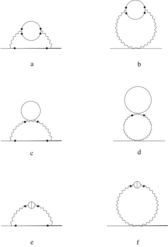
Figure 1: Diagrams  for  $\partial_{\mu}\hat{X}_{i}\partial_{\mu}\hat{X}^{i}$

In order to evaluate the divergences for the kinetic term of $\hat{X}_{i}$ , we have to consider six diagrams (Fig.1), where $\hat{h}_{\mu\nu}$ is set to be equal to zero. The results are obtained in the form

$$\frac{cG}{(4\pi)^{2}}\alpha\int\mbox{d}^{D}x\frac{1}{2}\partial_{\mu}\hat{X}_{i}\partial_{\mu}\hat{X}^{i},$$ (4.1)

and the coefficient $\alpha$ for each diagram is shown in Table 1. We can see that each of the diagrams gives a local single–pole divergence and has no infrared divergence. The final result is written in the covariant form as

$$\frac{cG}{(4\pi)^{2}}\biggl{(}-{1\over 8\epsilon}\biggr{)}\int\mbox{d}^{D}x\sqrt{\hat{g}}\hat{g}^{\mu\nu}\frac{1}{2}\partial_{\mu}\hat{X}_{i}\partial_{\nu}\hat{X}^{i}.$$ (4.2)

4.2 Divergences for $\hat{R}\ \hat{X}_{i}\hat{X}^{i}$

We write down all the diagrams which are of the first order in $\hat{h}_{\mu\nu}$ and subtract from them the contributions of $\hat{g}^{\mu\nu}\partial_{\mu}\hat{X}_{i}\partial_{\nu}\hat{X}^{i}$. Thus we obtain thirty–three diagrams, which is found to give the divergences of the form $\hat{R}\ \hat{X}_{i}\hat{X}^{i}$. Note here that since all the diagrams include a vertex proportional to $\epsilon b$, there is in principle neither nonlocal nor infrared divergence, though one may have a local single–pole divergence in general. We can, therefore, conclude that the theory is renormalizable with $L=1-{1\over 2}\epsilon bX_{i}X^{i}$ up to the two–loop level, though arbitrary polynomials of $X_{i}X^{i}$ may appear in $L$ at higher orders. A concrete calculation shows that only five diagrams provide nontrivial contributions, which cancel among them. Thus, as a result, we find no divergences for $\hat{R}\ \hat{X}_{i}\hat{X}^{i}$.

4.3 Divergences for $\hat{R}$

We set $\hat{X}_{i}=0$ and evaluate the two–point functions of $\hat{h}_{\mu\nu}$. The diagrams we have to calculate are classified into two categories. The first one consists of forty–one diagrams, which contain a vertex proportional to $\epsilon b$ and give only a local single–pole divergence in general. Among them, there are four diagrams with the ghost loop and each of them is found to give no contribution. As for the remaining thirty–seven diagrams, our calculation shows that all the nonvanishing contributions cancel among the diagrams.

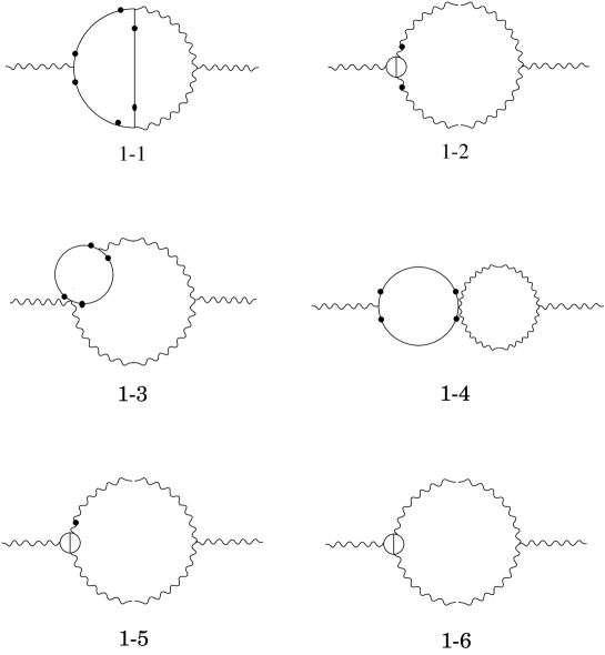
Figure 2: Diagrams  of  Group  1

The other category is a set of forty–three diagrams which possess no overall $\epsilon b$ factor and are able to give nonlocal as well as infrared divergences. We classify them into the thirteen groups (Fig.2–Fig.14), such that the contribution from each of them becomes local.

Groups $1,\ 2$ and $3$, as well as Group 5 to 11, are topologically the same, but differ in the vertices connected to the external $\hat{h}_{\mu\nu}$ lines. Except for Group 13, the one–loop counterterm insertion cancels the subdivergence from the matter subloop. On the other hand, the two diagrams of Group $13$ contain the subdiagrams which are the two–point functions of the matter fields at the one–loop level. As is seen in the one–loop calculation, the divergent contributions from these subdiagrams cancel each other, which implies that Group $13$ gives a local divergence without one–loop counterterm insertions. The calculations of the diagrams with the same topology as the diagram $1-1$ are carried out by the method presented in ref. [9].

We summarize the results for each of the Groups in Tables $2$ to $14$. We obtain generally the divergences in the momentum space as

$$\frac{cG}{(4\pi)^{2}}\int\frac{\mbox{d}^{D}k}{{(2\pi)}^{D}}\biggl{\{}Ak_{\mu}k_{\nu}\hat{h}(k)_{\mu\lambda}\hat{h}(-k)_{\nu\lambda}+Bk^{2}\hat{h}(k)_{\mu\nu}\hat{h}(-k)_{\mu\nu}$$ (4.3)

$$~{}~{}~{}~{}~{}~{}~{}~{}~{}~{}~{}~{}~{}~{}~{}~{}~{}~{}~{}~{}~{}+C\frac{1}{k^{2}}k_{\mu}k_{\nu}\hat{h}(k)_{\mu\nu}k_{\lambda}k_{\rho}\hat{h}(-k)_{\lambda\rho}\biggr{\}}.$$

The coefficients $A$, $B$ and $C$ are shown in the Tables. The $\rho$ and $\sigma$ in the Tables are defined as,

$$\rho=\log\left(\frac{k^{2}}{4\pi}\right),$$

$$\sigma=\log\left(\frac{m^{2}}{k^{2}}\right).$$

We can see that in the total of each of the Groups, $\rho$ and $\sigma$ do not appear and $C$ is equal to zero . This means that the nonlocal divergences as well as the infrared divergences in the $\frac{1}{\epsilon}$ pole cancel among the diagrams within each of the Groups. We also collect the total results of the Groups in Table $15$ and sum them up in the total. The double–pole singularity does vanish in the final result although it remains in each Group generically. From the relation between $A$ and $B$ in the final result and the formula (3.36), we can verify the preservation of the general covariance with respect to the background, which serves as a check of our calculation. The final result for the divergent contribution is found to be

$$\frac{cG}{{(4\pi)}^{2}}\frac{5}{24\epsilon}\int\mbox{d}^{D}x\sqrt{\hat{g}}\hat{R}.$$ (4.4)

5 Conformal Invariance and the Ultraviolet Fixed Point

In the previous section, we have calculated the divergences in the effective action and determined the counterterms by the background field method. The bare action can be written as

$$S_{0} = \int\mbox{d}^{D}x\sqrt{\hat{g}}\frac{\mu^{\epsilon}}{G}\left\{\left(1-\frac{25-c}{6\epsilon}\hat{G}+\frac{5c}{24\epsilon}\hat{G}^{2}\right)\tilde{R}\right.$$ (5.1)

$$~{}~{}~{}~{}~{}~{}~{}~{}~{}~{}~{}~{}~{}~{}~{}~{}~{}~{}~{}-\frac{1}{2}(\epsilon b-w\hat{G}^{2}b)X_{i}X^{i}\tilde{R}$$

$$~{}~{}~{}~{}~{}~{}~{}~{}~{}~{}~{}~{}~{}~{}~{}~{}~{}~{}~{}\left.+\frac{1}{2}\left(1-\frac{c}{8\epsilon}\hat{G}^{2}\right)\tilde{g}^{\mu\nu}\partial_{\mu}X_{i}\partial_{\nu}X^{i}\right\},$$

where $\hat{G}$ is equal to $G/4\pi$. We have introduced a parameter $w$ , which corresponds to a finite renormalization of the coupling $X_{i}X^{i}\tilde{R}$. Although it can be taken arbitrary as far as the divergence of the theory is concerned, we have to keep it since the corresponding tree–level coupling constant is $O(\epsilon)$.

We parametrize the bare action as

$$S_{0}=\frac{1}{G_{0}}\int\mbox{d}^{D}x\sqrt{\hat{g}}\left\{\left(1-\frac{1}{2}\epsilon b_{0}X_{0i}X_{0}^{~{}i}\right)\tilde{R}+\frac{1}{2}\tilde{g}^{\mu\nu}\partial_{\mu}X_{0i}\partial_{\nu}X_{0}^{~{}i}\right\},$$ (5.2)

which gives the following relations between the bare quantities and the renormalized quantities.

$$\frac{1}{G_{0}} = \frac{\mu^{\epsilon}}{G}\left(1-\frac{25-c}{6\epsilon}\hat{G}+\frac{5c}{24\epsilon}\hat{G}^{2}\right),$$ (5.3)

$$\epsilon b_{0} = \epsilon b+\left(\frac{c}{8}-w\right)\hat{G}^{2}b.$$ (5.4)

Using these relations, the $\beta$ functions can be obtained as

$$\beta_{G} = G\left(\epsilon-\frac{25-c}{6}\hat{G}+\frac{5c}{12}\hat{G}^{2}\right),$$ (5.5)

$$\beta_{b} = \left(2w-\frac{c}{4}\right)\hat{G}^{2}b.$$ (5.6)

The absence of the double pole at the two–loop level in (5.3) follows from the finiteness of $\beta_{G}$ just like in the Yang-Mills theory with the background gauge [10]. The absence of the single pole in (5.4) is also required for the the finiteness of $\beta_{b}$. This coupling constant always has an $\epsilon$ factor suppression due to the symmetry under the constant shift of the $X_{i}$ fields. One finds, in the expression for $\beta_{b}$, that the free parameter $w$ is relevant to the physics of the system. As we see in the following, this ambiguity will be fixed when we impose the general covariance on the bare action.

Since we have maintained only the volume–preserving diffeomorphism, we have to impose the conformal invariance on the bare action so that the theory is generally covariant. We consider the conformal transformation

$$\delta\tilde{g}_{\mu\nu} = \tilde{g}_{\mu\nu}\delta\rho,$$ (5.7)

$$\delta X_{0i} = (D-1)\frac{\partial L_{0}}{\partial X_{0}^{~{}i}}\delta\rho,$$ (5.8)

where $L_{0}=1-\frac{1}{2}\epsilon b_{0}X_{0i}X_{0}^{~{}i}$. Under this transformation, the bare action transforms as

$$\delta S_{0} = \int\mbox{d}^{D}x\sqrt{\hat{g}}\frac{\mu^{\epsilon}}{2G}\left[\left\{\epsilon-\frac{25-c}{6}\hat{G}+\frac{5c}{24}\hat{G}^{2}\right\}\tilde{R}\right.$$ (5.9)

$$-\frac{1}{2}\left\{\epsilon(\epsilon b-w\hat{G}^{2}b)-4(D-1)(\epsilon b-w\hat{G}^{2}b)\left(\epsilon-w\hat{G}^{2}+\frac{c}{8}\hat{G}^{2}\right)b\right\}X_{i}X^{i}\tilde{R}$$

$$+\left.\frac{1}{2}\left\{\epsilon\left(1-\frac{c}{8\epsilon}\hat{G}^{2}\right)-4(D-1)(\epsilon b-w\hat{G}^{2}b)\right\}\partial_{\mu}X_{i}\partial^{\mu}X^{i}\right]\delta\rho.$$

When we consider symmetry at the quantum level within the counterterm formalism, we have to replace the operators in (5.9) with the corresponding renormalized operators [11, 12, 13].

In order to define the renormalized operator for $X_{i}X^{i}\tilde{R}$, we differentiate the bare action with respect to the finite parameter $b$

$$\int\mbox{d}^{D}x\sqrt{\hat{g}}(X_{i}X^{i}\tilde{R})_{r}\equiv-\frac{2G}{\epsilon\mu^{\epsilon}}\frac{\partial S_{0}}{\partial b}=\left(1-\frac{w\hat{G}^{2}}{\epsilon}\right)\int\mbox{d}^{D}x\sqrt{\hat{g}}X_{i}X^{i}\tilde{R}.$$ (5.10)

We need to translate this relation into the local one, where, in general, one may have some total derivative terms. We note, however, that a complete set of operators can be written without total derivative terms by making use of the equations of motion [13]. We can, therefore, define the renormalized operator $(X_{i}X^{i}\tilde{R})_{r}$ as

$$(X_{i}X^{i}\tilde{R})_{r}=\left(1-\frac{w\hat{G}^{2}}{\epsilon}\right)X_{i}X^{i}\tilde{R}.$$ (5.11)

The same reasoning holds in the case of the other operators, which we omit to mention in the following.

The renormalized operator for $\partial_{\mu}X_{i}\partial^{\mu}X^{i}$ can be obtained by introducing a parameter “$f$” in front of the tree–level kinetic term of $X_{i}$ and keep track of the parameter in the divergent diagrams. The propagator of $X_{i}$ is multiplied by a factor $\frac{1}{f}$ and the vertices which originate from the kinetic term of $X_{i}$ are multiplied by a factor $f$. One finds that all the diagrams corresponding to the renormalization of the kinetic term are multiplied by a factor $f$ and the other diagrams remain the same. This implies that the renormalized operator for $\partial_{\mu}X_{i}\partial^{\mu}X^{i}$ can be defined through

$$\partial_{\mu}X_{i}\partial^{\mu}X^{i}=\left(1+\frac{c\hat{G}^{2}}{8\epsilon}\right)(\partial_{\mu}X_{i}\partial^{\mu}X^{i})_{r}.$$ (5.12)

Finally the renormalized operator for $\tilde{R}$ can be obtained as follows. We renormalize $X_{i}$ so that the only $G$ dependence comes from the coefficient of $\tilde{R}$ . Also we have to perform the wave function renormalization in order to avoid picking up unphysical contributions from the kinetic term of $X_{i}$. Thus we define

$$Y_{i}=\sqrt{\frac{1}{G}\left(1-\frac{c}{8\epsilon}\hat{G}^{2}\right)}X_{i},$$ (5.13)

and rewrite the action in terms of $Y_{i}$ as

$$S_{0}(G,Y_{i}) = \int\mbox{d}^{D}x\sqrt{\hat{g}}\mu^{\epsilon}\left[\frac{1}{G}\left(1-\frac{25-c}{6\epsilon}\hat{G}+\frac{5c}{24\epsilon}\hat{G}^{2}\right)\tilde{R}\right.$$ (5.14)

$$~{}~{}~{}~{}~{}~{}~{}~{}~{}~{}~{}~{}~{}~{}~{}~{}~{}-\frac{1}{2}\left(\epsilon b-w\hat{G}^{2}b+\frac{c}{8}\hat{G}^{2}b\right)Y_{i}Y^{i}\tilde{R}$$

$$~{}~{}~{}~{}~{}~{}~{}~{}~{}~{}~{}~{}~{}~{}~{}~{}~{}\left.+\frac{1}{2}\partial_{\mu}Y_{i}\partial^{\mu}Y^{i}\right].$$

By differentiating the above bare action with respect to $1/G$, we can obtain the renormalized operator for $\tilde{R}$ as

$$(\tilde{R})_{r}=\left(1-\frac{5c}{24\epsilon}\hat{G}^{2}\right)\tilde{R}-\left(w\hat{G}^{2}b-\frac{c}{8}\hat{G}^{2}b\right)X_{i}X^{i}\tilde{R}.$$ (5.15)

Using eqs. (5.11), (5.12) and (5.15), the conformal anomaly (5.9) can be written in terms of the renormalized operators as

$$\int\mbox{d}^{D}x\sqrt{\hat{g}}\frac{\mu^{\epsilon}}{2G}\left[\left\{\epsilon-\frac{25-c}{6}\hat{G}+\frac{5c}{12}\hat{G}^{2}\right\}(\tilde{R})_{r}\right.$$

$$~{}~{}~{}~{}~{}~{}~{}~{}~{}-\frac{1}{2}\epsilon b\left\{\epsilon-4(D-1)\left(\epsilon b-w\hat{G}^{2}b+\frac{c}{8}\hat{G}^{2}b\right)-2\left(w\hat{G}^{2}-\frac{c}{8}\hat{G}^{2}\right)\right\}(X_{i}X^{i}\tilde{R})_{r}$$

$$~{}~{}~{}~{}~{}~{}~{}~{}~{}-\left.\frac{1}{2}\left\{\epsilon-4(D-1)\left(\epsilon b-w\hat{G}^{2}b+\frac{c}{8}\hat{G}^{2}b\right)\right\}(\partial_{\mu}X_{i}\partial^{\mu}X^{i})_{r}\right]\delta\rho.$$ (5.16)

This result is reasonable since each term includes the expression for the $\beta$ function. At the ultraviolet fixed point, where the $\beta$ functions vanish, the conformal anomaly vanishes if and only if the fixed–point value of $b$ is given by

$$b=b^{\ast}=\frac{1}{4(D-1)}.$$ (5.17)

This is the same as the one–loop result. In order that this nonvanishing fixed–point value of $b$ may be realized, the coefficient $(2w-c/4)$ in the $\beta$ function of $b$ should vanish. Thus the free parameter $w$ should be chosen to be $\frac{c}{8}$ to the leading order of $c$. Note also that the fixed–point value of $b$ coincides with the value of $b$ that corresponds to the classical Einstein gravity. This is consistent with the one–loop result where it has been shown that the $\beta$ function of $b$ remains zero throughout the renormalization group trajectory from the ultraviolet fixed point to the infrared fixed point which corresponds to Einstein gravity.

6 Summary and Discussion

The recent progress in two-dimensional quantum gravity has provided us with an example of a consistent field theory with the general covariance. It is natural for us to hope that we can formulate quantum gravity near two dimensions by using the $\epsilon$ expansion. It has been discovered, however, that special care should be taken when we impose the general covariance on the theory in the renormalization procedure. It is because the general covariance inevitably relates the large scale physics to the short distance physics. This feature is not easy to reconcile with the idea of the renormalized field theory, where we consider the physics at a fixed scale.

Putting it in a slightly different way, the subtlety arises from the fact that in quantum gravity we integrate over the metric which serves to set the physical scale. We, therefore, have to consider all length scale at once. However in field theory, we need to introduce the short distance cutoff in some form, which inevitably breaks the general covariance. The conformal anomaly may be a manifestation of such difficulties. The oversubtraction problem [3, 4] and the conformal anomaly are the different faces of the same coin. In this sense we are dealing with a generic problem in quantum gravity which is not specific to the Einstein gravity near two dimensions.

The strategy adopted in ref. [5] was to take the tree action to be the most general one that is invariant under the volume–preserving diffeomorphism and to impose the full general covariance by choosing a renormalization group trajectory on which the conformal anomaly vanishes. At the one–loop level it has been shown that there exists such a trajectory which starts from an ultraviolet fixed point and flows into the classical Einstein gravity in the infrared limit. However, it is certainly nontrivial whether this idea works to all orders of the $\epsilon$ expansion. It is, therefore, desirable to see how it goes at the two–loop level. The results we have obtained in this paper are very encouraging. Although the conformal anomaly inevitably arises in quantum field theory, it is a short distance effect and always local. Therefore we should be able to cancel it by changing the coupling constants in the theory. Based on these reasonings, we expect that this program will succeed.

In this paper, we have studied two–loop renormalization imposing the $Z_{2}$ symmetry on the system. We have calculated the divergences proportional to the number of matter fields and examined how the nonlocal divergences as well as the infrared divergences in the $\frac{1}{\epsilon}$ pole cancel among the diagrams. It has been shown that the conformal anomaly vanishes at the ultraviolet fixed point when we choose the finite renormalization properly. This ensures the existence of the ultraviolet fixed point which possesses the general covariance up to the two–loop level in the leading order of $c$. We have to work out similar calculations without imposing the $Z_{2}$ symmetry on the system in order to examine the general covariance on the renormalization group trajectory that flows into the classical Einstein gravity. It seems also important for us to perform the full calculation of the two–loop renormalization without restricting ourselves to the leading matter contribution. We hope that we can eventually calculate physical quantities such as the critical exponents, which may be calculable also in numerical simulations of three or four dimensional quantum gravity in future.

We would like to thank H. Kawai and M. Ninomiya for stimulating discussion. Tremendous amount of tensor calculation involved in this work has been done with the aid of MathTensor, a software designed for symbolic manipulations in tensor analysis. It is our pleasure to acknowledge S. Christensen of MathSolution Inc. for his kind advice concerning the usage of this powerful tool.

Diagram	$a$	$b$	$c$	$d$	$e$	$f$	Total
$\alpha$	$0$	$\frac{1}{8\epsilon}$	$\frac{2b}{\epsilon}$	$-\frac{2b}{\epsilon}$	$-\frac{1}{12\epsilon}$	$-\frac{1}{6\epsilon}$	$-\frac{1}{8\epsilon}$

Table 1: The divergences for $\partial_{\mu}\hat{X}_{i}\partial_{\mu}\hat{X}^{i}$

Diagram	$A$	$B$	$C$
$1-1$	$-\frac{1}{4\epsilon^{2}}+(\frac{13}{48}-\frac{\gamma}{4}-\frac{\rho}{4}-\sigma)\frac{1}{\epsilon}$	$\frac{1}{8\epsilon^{2}}+(-\frac{13}{96}+\frac{\gamma}{8}+\frac{\rho}{8}+\frac{\sigma}{2})\frac{1}{\epsilon}$	$0$
$1-2$	$\frac{1}{2\epsilon^{2}}+(-\frac{4}{3}+\frac{\gamma}{4}+\frac{\rho}{4})\frac{1}{\epsilon}$	$-\frac{1}{4\epsilon^{2}}+(\frac{2}{3}-\frac{\gamma}{8}-\frac{\rho}{8})\frac{1}{\epsilon}$	$0$
$1-3$	$(\frac{13}{12}+\frac{\sigma}{3})\frac{1}{\epsilon}$	$(-\frac{13}{24}-\frac{\sigma}{6})\frac{1}{\epsilon}$	$0$
$1-4$	$\frac{\sigma}{2\epsilon}$	$-\frac{\sigma}{4\epsilon}$	$0$
$1-5$	$-\frac{\sigma}{2\epsilon}$	$\frac{\sigma}{4\epsilon}$	$\frac{\sigma}{3\epsilon}$
$1-6$	$\frac{2\sigma}{3\epsilon}$	$-\frac{\sigma}{3\epsilon}$	$-\frac{\sigma}{3\epsilon}$
Total	$\frac{1}{4\epsilon^{2}}+\frac{1}{48\epsilon}$	$-\frac{1}{8\epsilon^{2}}-\frac{1}{96\epsilon}$	$0$

Table 2: The results for Group $1$

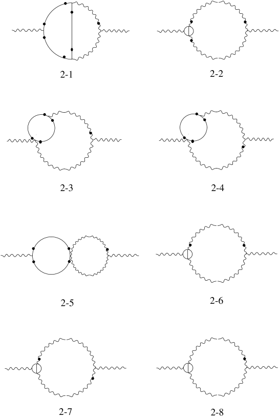
Figure 3: Diagrams  of  Group  2

Diagram	$A$	$B$	$C$
$2-1$	$-\frac{1}{4\epsilon^{2}}+(\frac{5}{16}-\frac{\gamma}{4}-\frac{\rho}{4})\frac{1}{\epsilon}$	$\frac{1}{8\epsilon^{2}}+(-\frac{7}{32}+\frac{\gamma}{8}+\frac{\rho}{8})\frac{1}{\epsilon}$	$0$
$2-2$	$-\frac{5}{6\epsilon^{2}}+(\frac{5}{12}-\frac{5\gamma}{12}-\frac{5\rho}{12})\frac{1}{\epsilon}$	$\frac{5}{12\epsilon^{2}}+(-\frac{1}{12}+\frac{5\gamma}{24}+\frac{5\rho}{24})\frac{1}{\epsilon}$	$0$
$2-3$	$\frac{1}{4\epsilon^{2}}+(-\frac{7}{48}+\frac{\gamma}{4}+\frac{\rho}{4}+\frac{\sigma}{2})\frac{1}{\epsilon}$	$-\frac{1}{8\epsilon^{2}}+(\frac{13}{96}-\frac{\gamma}{8}-\frac{\rho}{8}-\frac{\sigma}{4})\frac{1}{\epsilon}$	$0$
$2-4$	$-\frac{1}{4\epsilon^{2}}+(\frac{31}{48}-\frac{\gamma}{4}-\frac{\rho}{4})\frac{1}{\epsilon}$	$\frac{1}{8\epsilon^{2}}+(-\frac{37}{96}+\frac{\gamma}{8}+\frac{\rho}{8})\frac{1}{\epsilon}$	$0$
$2-5$	$0$	$0$	$0$
$2-6$	$\frac{2}{3\epsilon^{2}}+(-\frac{1}{6}+\frac{\gamma}{3}+\frac{\rho}{3})\frac{1}{\epsilon}$	$-\frac{1}{3\epsilon^{2}}+(\frac{1}{8}-\frac{\gamma}{6}-\frac{\rho}{6})\frac{1}{\epsilon}$	$0$
$2-7$	$\frac{2}{3\epsilon^{2}}+(-\frac{5}{6}+\frac{\gamma}{3}+\frac{\rho}{3})\frac{1}{\epsilon}$	$-\frac{1}{3\epsilon^{2}}+(\frac{11}{24}-\frac{\gamma}{6}-\frac{\rho}{6})\frac{1}{\epsilon}$	$0$
$2-8$	$-\frac{\sigma}{2\epsilon}$	$\frac{\sigma}{4\epsilon}$	$0$
Total	$\frac{1}{4\epsilon^{2}}+\frac{11}{48\epsilon}$	$-\frac{1}{8\epsilon^{2}}+\frac{1}{32\epsilon}$	$0$

Table 3: The results for Group $2$

Figure 4: Diagrams  of  Group  3

Diagram	$A$	$B$	$C$
$3-1$	$\frac{19}{24\epsilon}$	$-\frac{11}{24\epsilon}$	$0$
$3-2$	$\frac{11}{36\epsilon}$	$-\frac{5}{18\epsilon}$	$0$
$3-3$	$\frac{1}{2\epsilon^{2}}+(-\frac{4}{3}+\frac{\gamma}{2}+\frac{\rho}{2})\frac{1}{\epsilon}$	$-\frac{1}{4\epsilon^{2}}+(\frac{19}{24}-\frac{\gamma}{4}-\frac{\rho}{4})\frac{1}{\epsilon}$	$0$
$3-4$	$-\frac{1}{2\epsilon}$	$\frac{1}{4\epsilon}$	$0$
$3-5$	$\frac{2}{3\epsilon}$	$-\frac{1}{3\epsilon}$	$\frac{1}{6\epsilon}$
$3-6$	$-\frac{1}{\epsilon^{2}}+(\frac{1}{3}-\frac{\gamma}{2}-\frac{\rho}{2})\frac{1}{\epsilon}$	$\frac{1}{2\epsilon^{2}}+(-\frac{1}{6}+\frac{\gamma}{4}+\frac{\rho}{4})\frac{1}{\epsilon}$	$-\frac{1}{6\epsilon}$
Total	$-\frac{1}{2\epsilon^{2}}+\frac{19}{72\epsilon}$	$\frac{1}{4\epsilon^{2}}-\frac{7}{36\epsilon}$	$0$

Table 4: The results for Group $3$

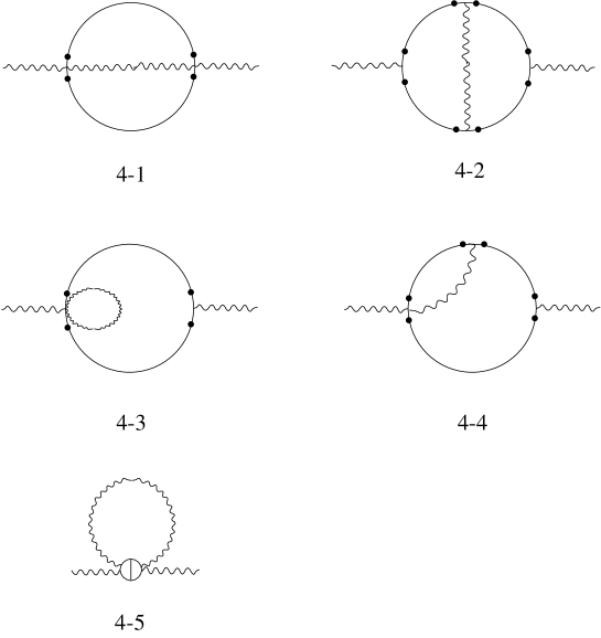
Figure 5: Diagrams  of  Group  4

Diagram	$A$	$B$	$C$
$4-1$	$-\frac{1}{2\epsilon^{2}}+(\frac{13}{24}-\frac{\gamma}{2}-\frac{\rho}{2}-\frac{\sigma}{2})\frac{1}{\epsilon}$	$\frac{1}{8\epsilon^{2}}+(-\frac{19}{48}+\frac{\gamma}{8}+\frac{\rho}{8}+\frac{\sigma}{8})\frac{1}{\epsilon}$	$0$
$4-2$	$\frac{1}{4\epsilon^{2}}+(-\frac{1}{16}+\frac{\gamma}{4}+\frac{\rho}{4}+\frac{\sigma}{4})\frac{1}{\epsilon}$	$-\frac{1}{4\epsilon^{2}}+(\frac{1}{32}-\frac{\gamma}{4}-\frac{\rho}{4}-\frac{\sigma}{4})\frac{1}{\epsilon}$	$0$
$4-3$	$\frac{1}{3\epsilon^{2}}+(\frac{11}{36}+\frac{\gamma}{3}+\frac{\rho}{3}+\frac{\sigma}{6})\frac{1}{\epsilon}$	$-\frac{1}{6\epsilon^{2}}+(-\frac{11}{72}-\frac{\gamma}{6}-\frac{\rho}{6}-\frac{\sigma}{12})\frac{1}{\epsilon}$	$-\frac{1}{6\epsilon}$
$4-4$	$-\frac{1}{3\epsilon^{2}}+(-\frac{13}{72}-\frac{\gamma}{3}-\frac{\rho}{3}-\frac{\sigma}{6})\frac{1}{\epsilon}$	$\frac{5}{12\epsilon^{2}}+(\frac{31}{144}+\frac{5\gamma}{12}+\frac{5\rho}{12}+\frac{\sigma}{3})\frac{1}{\epsilon}$	$\frac{1}{6\epsilon}$
$4-5$	$\frac{1}{2\epsilon^{2}}+(-\frac{7}{8}+\frac{\gamma}{4}+\frac{\rho}{4}+\frac{\sigma}{4})\frac{1}{\epsilon}$	$-\frac{1}{4\epsilon^{2}}+(\frac{19}{48}-\frac{\gamma}{8}-\frac{\rho}{8}-\frac{\sigma}{8})\frac{1}{\epsilon}$	$0$
Total	$\frac{1}{4\epsilon^{2}}-\frac{13}{48\epsilon}$	$-\frac{1}{8\epsilon^{2}}+\frac{3}{32\epsilon}$	$0$

Table 5: The results for Group $4$

Figure 6: Diagrams  of  Group  5

Diagram	$A$	$B$	$C$
$5-1$	$-\frac{1}{8\epsilon^{2}}+(\frac{13}{32}-\frac{\gamma}{8}-\frac{\rho}{8})\frac{1}{\epsilon}$	$\frac{1}{16\epsilon^{2}}+(-\frac{19}{64}+\frac{\gamma}{16}+\frac{\rho}{16})\frac{1}{\epsilon}$	$0$
$5-2$	$\frac{1}{4\epsilon^{2}}+(-\frac{17}{36}+\frac{\gamma}{8}+\frac{\rho}{8})\frac{1}{\epsilon}$	$-\frac{1}{8\epsilon^{2}}+(\frac{61}{144}-\frac{\gamma}{16}-\frac{\rho}{16})\frac{1}{\epsilon}$	$0$
Total	$\frac{1}{8\epsilon^{2}}-\frac{19}{288\epsilon}$	$-\frac{1}{16\epsilon^{2}}+\frac{73}{576\epsilon}$	$0$

Table 6: The results for Group $5$

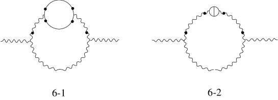
Figure 7: Diagrams  of  Group  6

Diagram	$A$	$B$	$C$
$6-1$	$(-\frac{13}{192}-\frac{\sigma}{8})\frac{1}{\epsilon}$	$(\frac{7}{384}+\frac{\sigma}{16})\frac{1}{\epsilon}$	$0$
$6-2$	$(\frac{1}{48}+\frac{\sigma}{8})\frac{1}{\epsilon}$	$-\frac{\sigma}{16}$	$0$
Total	$-\frac{3}{64\epsilon}$	$\frac{7}{384\epsilon}$	$0$

Table 7: The results for Group $6$

Figure 8: Diagrams  of  Group  7

Diagram	$A$	$B$	$C$
$7-1$	$\frac{11}{192\epsilon}$	$-\frac{29}{384\epsilon}$	$0$
$7-2$	$-\frac{5}{48\epsilon}$	$\frac{1}{8\epsilon}$	$0$
Total	$-\frac{3}{64\epsilon}$	$\frac{19}{384\epsilon}$	$0$

Table 8: The results for Group $7$

Figure 9: Diagrams  of  Group  8

Diagram	$A$	$B$	$C$
$8-1$	$\frac{1}{8\epsilon^{2}}+(-\frac{13}{48}+\frac{\gamma}{8}+\frac{\rho}{8})\frac{1}{\epsilon}$	$-\frac{1}{16\epsilon^{2}}+(\frac{5}{48}-\frac{\gamma}{16}-\frac{\rho}{16})\frac{1}{\epsilon}$	$0$
$8-2$	$-\frac{1}{4\epsilon^{2}}+(\frac{5}{24}-\frac{\gamma}{8}-\frac{\rho}{8})\frac{1}{\epsilon}$	$\frac{1}{8\epsilon^{2}}+(-\frac{1}{12}+\frac{\gamma}{16}+\frac{\rho}{16})\frac{1}{\epsilon}$	$0$
Total	$-\frac{1}{8\epsilon^{2}}-\frac{1}{16\epsilon}$	$\frac{1}{16\epsilon^{2}}+\frac{1}{48\epsilon}$	$0$

Table 9: The results for Group $8$

  

Figure 10: Diagrams  of  Group  9

Diagram	$A$	$B$	$C$
$9-1$	$\frac{1}{4\epsilon^{2}}+(-\frac{25}{16}+\frac{\gamma}{4}+\frac{\rho}{4})\frac{1}{\epsilon}$	$-\frac{1}{8\epsilon^{2}}+(\frac{25}{32}-\frac{\gamma}{8}-\frac{\rho}{8})\frac{1}{\epsilon}$	$0$
$9-2$	$-\frac{1}{2\epsilon^{2}}+(\frac{5}{3}-\frac{\gamma}{4}-\frac{\rho}{4})\frac{1}{\epsilon}$	$\frac{1}{4\epsilon^{2}}+(-\frac{5}{6}+\frac{\gamma}{8}+\frac{\rho}{8})\frac{1}{\epsilon}$	$0$
Total	$-\frac{1}{4\epsilon^{2}}+\frac{5}{48\epsilon}$	$\frac{1}{8\epsilon^{2}}-\frac{5}{96\epsilon}$	$0$

Table 10: The results for Group $9$

Figure 11: Diagrams  of  Group  10

Diagram	$A$	$B$	$C$
$10-1$	$-\frac{1}{8\epsilon^{2}}+(\frac{13}{32}-\frac{\gamma}{8}-\frac{\rho}{8})\frac{1}{\epsilon}$	$\frac{1}{16\epsilon^{2}}+(-\frac{11}{64}+\frac{\gamma}{16}+\frac{\rho}{16})\frac{1}{\epsilon}$	$0$
$10-2$	$\frac{1}{4\epsilon^{2}}+(-\frac{11}{24}+\frac{\gamma}{8}+\frac{\rho}{8})\frac{1}{\epsilon}$	$-\frac{1}{8\epsilon^{2}}+(\frac{1}{6}-\frac{\gamma}{16}-\frac{\rho}{16})\frac{1}{\epsilon}$	$0$
Total	$\frac{1}{8\epsilon^{2}}-\frac{5}{96\epsilon}$	$-\frac{1}{16\epsilon^{2}}-\frac{1}{192\epsilon}$	$0$

Table 11: The results for Group $10$

Figure 12: Diagrams  of  Group  11

Diagram	$A$	$B$	$C$
$11-1$	$\frac{1}{8\epsilon^{2}}+(-\frac{13}{32}+\frac{\gamma}{8}+\frac{\rho}{8})\frac{1}{\epsilon}$	$-\frac{1}{16\epsilon^{2}}+(\frac{19}{64}-\frac{\gamma}{16}-\frac{\rho}{16})\frac{1}{\epsilon}$	$0$
$11-2$	$-\frac{1}{4\epsilon^{2}}+(\frac{11}{24}-\frac{\gamma}{8}-\frac{\rho}{8})\frac{1}{\epsilon}$	$\frac{1}{8\epsilon^{2}}+(-\frac{5}{12}+\frac{\gamma}{16}+\frac{\rho}{16})\frac{1}{\epsilon}$	$0$
Total	$-\frac{1}{8\epsilon^{2}}+\frac{5}{96\epsilon}$	$\frac{1}{16\epsilon^{2}}-\frac{23}{192\epsilon}$	$0$

Table 12: The results for Group $11$

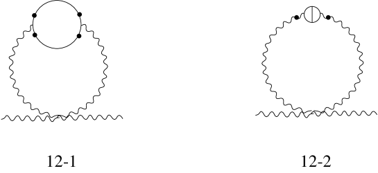
Figure 13: Diagrams  of  Group  12

Diagram	$A$	$B$	$C$
$12-1$	$\frac{5}{16\epsilon}$	$-\frac{3}{32\epsilon}$	$0$
$12-2$	$-\frac{5}{12\epsilon}$	$\frac{1}{8\epsilon}$	$0$
Total	$-\frac{5}{48\epsilon}$	$\frac{1}{32\epsilon}$	$0$

Table 13: The results for Group $12$

Figure 14: Diagrams  of  Group  13

Diagram	$A$	$B$	$C$
$13-1$	$\frac{1}{3\epsilon^{2}}+(-\frac{23}{72}+\frac{\gamma}{3}+\frac{\rho}{3}+\frac{\sigma}{6})\frac{1}{\epsilon}$	$-\frac{1}{6\epsilon^{2}}+(\frac{23}{144}-\frac{\gamma}{6}-\frac{\rho}{6}-\frac{\sigma}{12})\frac{1}{\epsilon}$	$-\frac{1}{6\epsilon}$
$13-2$	$-\frac{1}{3\epsilon^{2}}+(\frac{7}{36}-\frac{\gamma}{3}-\frac{\rho}{3}-\frac{\sigma}{6})\frac{1}{\epsilon}$	$\frac{1}{6\epsilon^{2}}+(-\frac{7}{72}+\frac{\gamma}{6}+\frac{\rho}{6}+\frac{\sigma}{12})\frac{1}{\epsilon}$	$\frac{1}{6\epsilon}$
Total	$-\frac{1}{8\epsilon}$	$\frac{1}{16\epsilon}$	$0$

Table 14: The results for Group $13$

Group	$A$	$B$
$1$	${1\over 4\epsilon^{2}}+{1\over 48\epsilon}$	$-{1\over 8\epsilon^{2}}-{1\over 96\epsilon}$
$2$	${1\over 4\epsilon^{2}}+{11\over 48\epsilon}$	$-{1\over 8\epsilon^{2}}+{1\over 32\epsilon}$
$3$	$-{1\over 2\epsilon^{2}}+{19\over 72\epsilon}$	${1\over 4\epsilon^{2}}-{7\over 36\epsilon}$
$4$	${1\over 4\epsilon^{2}}-{13\over 48\epsilon}$	$-{1\over 8\epsilon^{2}}+{3\over 32\epsilon}$
$5$	${1\over 8\epsilon^{2}}-{19\over 288\epsilon}$	$-{1\over 16\epsilon^{2}}+{73\over 576\epsilon}$
$6$	$-{3\over 64\epsilon}$	${7\over 384\epsilon}$
$7$	$-{3\over 64\epsilon}$	${19\over 384\epsilon}$
$8$	$-{1\over 8\epsilon^{2}}-{1\over 16\epsilon}$	${1\over 16\epsilon^{2}}+{1\over 48\epsilon}$
$9$	$-{1\over 4\epsilon^{2}}+{5\over 48\epsilon}$	${1\over 8\epsilon^{2}}-{5\over 96\epsilon}$
$10$	${1\over 8\epsilon^{2}}-{5\over 96\epsilon}$	$-{1\over 16\epsilon^{2}}-{1\over 192\epsilon}$
$11$	$-{1\over 8\epsilon^{2}}+{5\over 96\epsilon}$	${1\over 16\epsilon^{2}}-{23\over 192\epsilon}$
$12$	$-{5\over 48\epsilon}$	${1\over 32\epsilon}$
$13$	$-{1\over 8\epsilon}$	${1\over 16\epsilon}$
Total	$-{5\over 48\epsilon}$	${5\over 96\epsilon}$

Table 15: Divergences for $\hat{R}$

References

-
[1]
S. Weinberg, in General Relativity, an Einstein Centenary
Survey, eds. S.W. Hawking and W. Israel (Cambridge
University Press, 1979).
R. Gastmans, R. Kallosh and C. Truffin, Nucl. Phys. B133 (1978) 417.
S.M. Christensen and M.J. Duff, Phys. Lett. B79 (1978) 213. - [2] H. Kawai and M. Ninomiya, Nucl. Phys. B336 (1990)115.
- [3] H. Kawai, Y. Kitazawa and M. Ninomiya, Nucl. Phys. B393(1993) 280.
- [4] H. Kawai, Y. Kitazawa and M. Ninomiya, Nucl. Phys. B404 (1993) 684.
- [5] T. Aida, Y. Kitazawa, H. Kawai and M. Ninomiya, Nucl. Phys. B427 (1994) 158.
- [6] J. Nishimura, S. Tamura and A. Tsuchiya, UT-664,ICRR-Report-308-94-1,UT-Komaba/94-2, to appear in Int. J. Mod. Phys. A.
- [7] J. Nishimura, S. Tamura and A. Tsuchiya, KEK-TH-394,ICRR-Report-318-94-13,UT-Komaba/94-11, to appear in Mod. Phys. Lett. A.
-
[8]
S.-I. Kojima, N. Sakai and Y. Tanii, TIT preprint, TIT-HEP-238,
November 1993, hep-th 9311045.
Y. Tanii, S.-I. Kojima and N. Sakai, Phys. Lett. B322 (1994) 59. - [9] C. Itzykson and J.-B. Zuber, ”Quantum Field Theory” (McGraw-Hill, Inc., 1980) p. 415
- [10] L.F. Abbott, Nucl. Phys. B185 (1981) 189.
- [11] C.G. Callan, D. Friedan, E.J. Martinec and M.J. Perry, Nucl. Phys. B262 (1985) 593.
- [12] E.S. Fradkin and A.A. Tseytlin, Nucl. Phys. B261 (1985) 1.
- [13] A.A. Tseytlin, Nucl. Phys. B294 (1987) 383.