NSF-ITP-94-97

hep-th/9411028

ABSTRACT

Lectures presented at the 1994 Les Houches Summer School “Fluctuating Geometries in Statistical Mechanics and Field Theory.” The first part is an introduction to conformal field theory and string perturbation theory. The second part deals with the search for a deeper answer to the question posed in the title.

While I was planning these lectures I happened to reread Ken Wilson’s account of his early work[2], and was struck by the parallel between string theory today and quantum field theory thirty years ago. Then, as now, one had a good technical control over the perturbation theory but little else. Wilson saw himself as asking the question “What is quantum field theory?” I found it enjoyable and inspiring to read about the various models he studied and approximations he tried (he refers to “clutching at straws”) before he found the simple and powerful answer, that the theory is to be organized scale-by-scale rather than graph-by-graph. That understanding made it possible to answer both problems of principle, such as how quantum field theory is to be defined beyond perturbation theory, and practical problems, such as how to determine the ground states and phases of quantum field theories.

In string theory today we have these same kinds of problems, and I think there is good reason to expect that an equally powerful organizing principle remains to be found. There are many reasons, as I will touch upon later, to believe that string theory is the correct unification of gravity, quantum mechanics, and particle physics. It is implicit, then, that the theory actually exists, and ‘exists’ does not mean just perturbation theory. The nature of the organizing principle is at this point quite open, and may be very different from what we are used to in quantum field theory.

One can ask whether the situation today in string theory is really as favorable as it was for field theory in the early 60’s. It is difficult to know. Then, of course, we had many more experiments to tell us how quantum field theories actually behave. To offset that, we have today more experience and greater mathematical sophistication. As an optimist, I make an encouraging interpretation of the history, that many of the key advances in field theory—Wilson’s renormalization group, the discovery of spontaneously broken gauge symmetry as the theory of the electroweak interaction, the discovery of general relativity itself—were carried out largely by study of simple model systems and limiting behaviors, and by considerations of internal consistency. These same tools are available in string theory today.

My lectures divide into two parts—an introduction to string theory as we now understand it, and a look at attempts to go further. For the introduction, I obviously cannot in five lectures cover the whole of superstring theory. Given time limitations, and given the broad range of interests among the students, I will try to focus on general principles. I will begin with conformal field theory (2.5 lectures), which of course has condensed matter applications as well as being the central tool in string theory. Section 2 (2.5 lectures) introduces string theory itself. Section 3 (1 lecture), on dualities and equivalences, covers the steadily increasing evidence that what appear to be different string theories are in many cases different ground states of a single theory. Section 4 (1 lecture) addresses the question of whether ‘string field theory’ is the organizing principle we seek. In section 5 (2 lectures) I discuss matrix models, exactly solvable string theories in low spacetime dimensions.

I should emphasize that this is a survey of many subjects rather than a review of any single subject (for example $R$-duality, on which I spend half a lecture, was the subject of a recent review [3] with nearly 300 references). I made an effort to choose references which will be useful to the student—a combination of reviews, some original references, and some interesting recent papers.

1 Conformal Field Theory

Much of the material in this lecture, especially the first part, is standard and can be found in many reviews. The 1988 Les Houches lectures by Ginsparg [4] and Cardy [5] focus on conformal field theory, the latter with emphasis on applications in statistical mechanics. Introductions to string theory with emphasis on conformal field theory can be found in refs. [6]-[10]. There are a number of recent books on string theory, though often with less emphasis on conformal techniques [11]-[15] as well as a book [16] and reprint collection [17] on conformal field theory and statistical mechanics. Those who are in no great hurry will eventually find an expanded version of these lectures in ref. [18]. Finally I should mention the seminal papers [19] and [20].

1.1 The Operator Product Expansion

The operator product expansion (OPE) plays a central role in this subject. I will introduce it using the example of a free scalar field in two dimensions, $X(\sigma^{1},\sigma^{2})$. I will focus on two dimensions because this is the case that will be of interest for the string, and I will refer to these two dimensions as ‘space’ though later they will be the string world-sheet and space will be something else. The action is

$$S=\frac{1}{8\pi}\int d^{2}\sigma\,\Bigl{\{}(\partial_{1}X)^{2}+(\partial_{2}X)^{2}\Bigr{\}}.$$ (1.1.1)

The normalization of the field $X$ (and so the action) is for later convenience. To be specific I have taken two Euclidean dimensions, but almost everything, at least until we get to nontrivial topologies, can be continued immediately to the Minkowski case $\sigma^{2}\to-i\sigma^{0}$. Expectation values are defined by the functional integral

$$<{\cal F}[X]>\ =\ \int[dX]\,e^{-S}{\cal F}[X],$$ (1.1.2)

where ${\cal F}[X]$ is any functional of $X$, such as a product of local operators.

It is very convenient to adopt complex coordinates

$$z=\sigma^{1}+i\sigma^{2},\qquad\bar{z}=\sigma^{1}-i\sigma^{2}.$$ (1.1.3)

Define also

$$\partial_{z}=\frac{1}{2}(\partial_{1}-i\partial_{2}),\qquad\partial_{\bar{z}}=\frac{1}{2}(\partial_{1}+i\partial_{2}).$$ (1.1.4)

These have the properties $\partial_{z}z=1$, $\partial_{z}\bar{z}=0$, and so on. Note also that $d^{2}z=2d\sigma^{1}d\sigma^{2}$ from the Jacobian, and that $\int d^{2}z\,\delta^{2}(z,\bar{z})=1$. I will further abbreviate $\partial_{z}$ to $\partial$ and $\partial_{\bar{z}}$ to $\bar{\partial}$ when this will not be ambiguous. For a general vector, define as above

$$v^{z}=v^{1}+iv^{2},\qquad v^{\bar{z}}=v^{1}-iv^{2},\qquad v_{z}=\frac{1}{2}(v^{1}-iv^{2}),\qquad v_{\bar{z}}=\frac{1}{2}(v^{1}+iv^{2}).$$ (1.1.5)

For the indices 1, 2 the metric is the identity and we do not distinguish between upper and lower, while the complex indices are raised and lowered with

$$g_{z\bar{z}}=g_{\bar{z}z}=\frac{1}{2},\qquad g_{zz}=g_{\bar{z}\bar{z}}=0,\qquad g^{z\bar{z}}=g^{\bar{z}z}=2,\qquad g^{zz}=g^{\bar{z}\bar{z}}=0$$ (1.1.6)

The action is then

$$S=\frac{1}{4\pi}\int d^{2}z\,\partial X\bar{\partial}X,$$ (1.1.7)

and the equation of motion is

$$\partial\bar{\partial}X(z,\bar{z})=0.$$ (1.1.8)

The notation $X(z,\bar{z})$ may seem redundant, since the value of $z$ determines the value of $\bar{z}$, but it is useful to reserve the notation $f(z)$ for fields whose equation of motion makes them analytic in $z$. For example, it follows at once from the equation of motion (1.1.8) that $\partial X$ is analytic and that $\bar{\partial}X$ is antianalytic (analytic in $\bar{z}$), hence the notations $\partial X(z)$ and $\bar{\partial}X(\bar{z})$. Notice that under the Minkowski continuation, an analytic field becomes left-moving, a function only of $\sigma^{0}+\sigma^{1}$, while an antianalytic field becomes right-moving, a function only of $\sigma^{0}-\sigma^{1}$.

Now, using the property of path integrals that the integral of a total derivative is zero, we have

$$0 = \int[dX]\,\frac{\delta}{\delta X(z,\bar{z})}\Bigl{\{}e^{-S}X(z^{\prime},\bar{z}^{\prime})\Bigr{\}}$$ (1.1.9)

$$= \int[dX]\,e^{-S}\Bigl{\{}\delta^{2}(z-z^{\prime},\bar{z}-\bar{z}^{\prime})+\frac{1}{2\pi}\partial_{z}\partial_{\bar{z}}X(z,\bar{z})X(z^{\prime},\bar{z}^{\prime})\Bigr{\}}$$

$$= <\delta^{2}(z-z^{\prime},\bar{z}-\bar{z}^{\prime})>+\frac{1}{2\pi}\partial_{z}\partial_{\bar{z}}<X(z,\bar{z})X(z^{\prime},\bar{z}^{\prime})>$$

That is, the equation of motion holds except at coincident points. Now, the same calculation goes through if we have arbitrary additional insertions ‘$\ldots$’ in the path integral, as long as no other fields are at $(z,\bar{z})$ or $(z^{\prime},\bar{z}^{\prime})$:

$$\frac{1}{2\pi}\partial_{z}\partial_{\bar{z}}<X(z,\bar{z})X(z^{\prime},\bar{z}^{\prime})\ldots>\ =\ -<\delta^{2}(z-z^{\prime},\bar{z}-\bar{z}^{\prime})\ldots>.$$ (1.1.10)

A relation which holds in this sense will simply be written

$$\frac{1}{2\pi}\partial_{z}\partial_{\bar{z}}X(z,\bar{z})X(z^{\prime},\bar{z}^{\prime})=-\delta^{2}(z-z^{\prime},\bar{z}-\bar{z}^{\prime}),$$ (1.1.11)

and will be called an operator equation. One can think of the additional fields ‘$\ldots$’ as preparing arbitrary initial and final states, so if one cuts the path integral open to make an Hamiltonian description, an operator equation is simply one which holds for arbitrary matrix elements. Note also that because of the way the path integral is constructed from iterated time slices, any product of fields in the path integral goes over to a time-ordered product in the Hamiltonian form. In the Hamiltonian formalism, the delta-function in eq. (1.1.11) comes from the differentiation of the time-ordering.

Now we define a very useful combinatorial tool, normal ordering:

$${:\!X(z,\bar{z})X(z^{\prime},\bar{z}^{\prime})\!:}\ \equiv\ X(z,\bar{z})X(z^{\prime},\bar{z}^{\prime})+\ln|z-z^{\prime}|^{2}.$$ (1.1.12)

The logarithm satisfies the equation of motion (1.1.11) with the opposite sign (the action was normalized such that this log would have coefficient 1), so that by construction

$$\partial_{z}\partial_{\bar{z}}{:\!X(z,\bar{z})X(z^{\prime},\bar{z}^{\prime})\!:}=0.$$ (1.1.13)

That is, the normal ordered product satisfies the naive equation of motion. This implies that the normal ordered product is locally the sum of an analytic and antianalytic function (a standard result from complex analysis). Thus it can be Taylor expanded, and so from the definition (1.1.12) we have (putting one operator at the origin for convenience)

$$X(z,\bar{z})X(0,0)=-\ln|z|^{2}\ +:\!X^{2}(0,0)\!:+\ z:\!X\partial X(0,0)\!:+\ \bar{z}:\!X\bar{\partial}X(0,0)\!:+\ldots\ .$$ (1.1.14)

This is an operator equation, in the same sense as the preceding equations.

Eq. (1.1.14) is our first example of an operator product expansion. For a general expectation value involving $X(z,\bar{z})X(0,0)$ and other fields, it gives the small-$z$ behavior as a sum of terms, each of which is a known function of $z$ times the expectation values of a single local operator. For a general field theory, denote a complete set of local operators for a field theory by ${\cal A}_{i}$. The OPE then takes the general form

$${\cal A}_{i}(z,\bar{z}){\cal A}_{j}(0,0)=\sum_{k}c^{k}\!_{ij}(z,\bar{z}){\cal A}_{k}(0,0).$$ (1.1.15)

Later in section 1 I will give a simple derivation of the OPE (1.1.15), and of a rather broad generalization of it. OPE’s are frequently used in particle and condensed matter physics as asymptotic expansions, the first few terms giving the dominant behavior at small $z$. However, I will argue that, at least in conformally invariant theories, the OPE is actually a convergent series. The radius of convergence is given by the distance to the nearest other operator in the path integral. Because of this the coefficient functions $c^{k}\!_{ij}(z,\bar{z})$, which as we will see must satisfy various further conditions, will enable us to reconstruct the entire field theory.
Exercise: The expectation value $<X(z_{1},\bar{z}_{1})X(z_{2},\bar{z}_{2})X(z_{3},\bar{z}_{3})X(z_{4},\bar{z}_{4})>$ is given by the sum over all Wick contractions with the propagator $-\ln|z_{i}-z_{j}|^{2}$. Compare the asymptotics as $z_{1}\to z_{2}$ from the OPE (1.1.14) with the asymptotics of the exact expression. Verify that the expansion in $z_{1}-z_{2}$ has the stated radius of convergence.

The various operators on the right-hand side of the OPE (1.1.14) involve products of fields at the same point. Usually in quantum field theory such a product is divergent and must be appropriately cut off and renormalized, but here the normal ordering renders it well-defined. Normal ordering is thus a convenient way to define composite operators in free field theory. It is of little use in most interacting field theories, because these have additional divergences from interaction vertices approaching the composite operator or one another. But many of the conformal field theories that we will be interested in are free, and many others can be related to free field theories, so it will be worthwhile to develop normal ordering somewhat further.

For products of more than 2 fields the definition (1.1.12) can be extended iteratively,

$${:\!X(z,\bar{z})X(z_{1},\bar{z}_{1})\ldots X(z_{n},\bar{z}_{n})\!:}\ \equiv\ X(z,\bar{z})\,\,{:\!X(z_{1},\bar{z}_{1})\ldots X(z_{n},\bar{z}_{n})\!:}$$ (1.1.16)

$$\qquad\qquad+\ \Bigl{\{}\ln|z-z_{1}|^{2}:\!X(z_{2},\bar{z}_{2})\ldots X(z_{n},\bar{z}_{n})\!:\ +\ (n-1){\rm\ permutations}\Bigr{\}},$$

contracting each pair (omitting the pair and subtracting $-\ln|z-z_{i}|^{2}$). This has the same properties as before: the equation of motion holds inside the normal ordering, and so the normal-ordered product is smooth. (Exercise: Show this. The simplest argument I have found is inductive, and uses the definition twice to pull both $X(z,\bar{z})$ and $X(z_{1},\bar{z}_{1})$ out of the normal ordering.)

The definition (1.1.16) can be written more formally as

$$:\!X(z,\bar{z}){\cal F}[X]\!:\ =X(z,\bar{z}):\!{\cal F}[X]\!:+\int d^{2}z^{\prime}\,\ln|z-z^{\prime}|^{2}\frac{\delta}{\delta X(z^{\prime},\bar{z}^{\prime})}:\!{\cal F}[X]\!:,$$ (1.1.17)

for an arbitrary functional ${\cal F}[X]$, the integral over the functional derivative producing all contractions. Finally, the definition of normal ordering can be written in a closed form by the same strategy,

$$:\!{\cal F}[X]\!:\ =\exp\biggl{\{}\frac{1}{2}\int d^{2}z\,d^{2}z^{\prime}\,\ln|z-z^{\prime}|^{2}\frac{\delta}{\delta X(z,\bar{z})}\frac{\delta}{\delta X(z^{\prime},\bar{z}^{\prime})}\biggr{\}}{\cal F}[X].$$ (1.1.18)

The exponential sums over all ways of contracting zero, one, two, or more pairs. The operator product of two normal ordered operators can be represented compactly as

$$:\!{\cal F}[X]\!:\,\,:\!{\cal G}[X]\!:\ =\exp\biggl{\{}-\int d^{2}z^{\prime}\,d^{2}z^{\prime\prime}\,\ln|z^{\prime}-z^{\prime\prime}|^{2}\frac{\delta_{F}}{\delta X(z^{\prime},\bar{z}^{\prime})}\frac{\delta_{G}}{\delta X(z^{\prime\prime},\bar{z}^{\prime\prime})}\biggr{\}}:\!{\cal F}[X]\,{\cal G}[X]\!:,$$ (1.1.19)

where $\delta_{F}$ and $\delta_{G}$ act only on the fields in ${\cal F}$ and ${\cal G}$ respectively. The expressions $:\!{\cal F}[X]\!:\,:\!{\cal G}[X]\!:$ and $:\!{\cal F}[X]\,{\cal G}[X]\!:$ differ by the contractions between one field from ${\cal F}$ and one field from ${\cal G}$, which are then restored by the exponential. Now, for ${\cal F}$ a local operator at $z_{1}$ and ${\cal G}$ a local operator at $z_{2}$, we can expand in $z_{1}-z_{2}$ inside the normal ordering on the right to generate the OPE. For example, one finds

$$:\!e^{ik_{1}X(z,\bar{z})}\!:\,\,:\!e^{ik_{2}X(0,0)}\!: = |z|^{2k_{1}k_{2}}:\!e^{ik_{1}X(z,\bar{z})+ik_{2}X(0,0)}\!:$$ (1.1.20)

$$\sim |z|^{2k_{1}k_{2}}:\!e^{i(k_{1}+k_{2})X(0,0)}\!:\ ,$$

since each contraction gives $k_{1}k_{2}\ln|z|^{2}$ and the contractions exponentiate. Exponential operators will be quite useful to us. Another example is

$$\partial X(z,\bar{z})\,:\!e^{ikX(0,0)}\!:\ \sim\ -\frac{ik}{z}:\!e^{ikX(0,0)}\!:\ ,$$ (1.1.21)

coming from a single contraction.

1.2 Ward Identities

The action (1.1.7) has a number of important symmetries, in particular conformal invariance. Let us first derive the Ward identities for a general symmetry. Suppose we have fields $\phi_{\alpha}(\sigma)$ with some action $S[\phi]$, and a symmetry

$$\phi^{\prime}_{\alpha}(\sigma)=\phi_{\alpha}(\sigma)+\epsilon\delta\phi_{\alpha}(\sigma).$$ (1.2.1)

That is, the product of the path integral measure and the weight $e^{-S}$ is invariant. For a path integral with general insertion ${\cal F}[\phi]$, make the change of variables (1.2.1). The invariance of the integral under change of variables, and the invariance of the measure times $e^{-S}$, give

$$0\ =\ \int d^{2}\sigma\,\sum_{\alpha}<\delta\phi_{\alpha}(\sigma)\frac{\delta}{\delta\phi_{\alpha}(\sigma)}{\cal F}[\phi]>\ \equiv\ <\delta{\cal F}[\phi]>.$$ (1.2.2)

This simply states that the general expectation value is invariant under the symmetry.

We can derive additional information from the symmetry: the existence of a conserved current (Noether’s theorem), and Ward identities for the expectation values of the current. Consider the following change of variables,

$$\phi^{\prime}_{\alpha}(\sigma)=\phi_{\alpha}(\sigma)+\epsilon\rho(\sigma)\delta\phi_{\alpha}(\sigma).$$ (1.2.3)

This is not a symmetry, the transformation law being altered by the inclusion of an arbitrary function $\rho(\sigma)$. The path integral measure times $e^{-S}$ would be invariant if $\rho$ were a constant, so its variation must be proportional to the gradient $\partial_{a}\rho$. Making the change of variables (1.2.3) in the path integral thus gives

$$0 = \int[d\phi^{\prime}]\,e^{-S[\phi^{\prime}]}-\int[d\phi]\,e^{-S[\phi]}$$ (1.2.4)

$$= \frac{i\epsilon}{2\pi}\int[d\phi]\,e^{-S[\phi]}\int d^{2}\sigma\,j^{a}(\sigma)\partial_{a}\rho(\sigma).$$

The unknown coefficient $j^{a}(\sigma)$ comes from the variation of the measure and the action, both of which are local, and so it must be a local function of the fields and their derivatives. Taking the function $\rho$ to be nonzero only in a small region allows us to integrate by parts; also, the identity (1.2.4) remains valid if we add arbitrary distant insertions ‘$\ldots$’. We thus derive

$$\partial_{a}j^{a}=0$$ (1.2.5)

as an operator equation. This is Noether’s theorem.
Exercise: Use this to derive the classical Noether theorem in the form usually found in textbooks. That is, assume that $S[\phi]=\int d^{2}\sigma\,L(\phi(\sigma),\partial_{a}\phi(\sigma))$ and ignore the variation of the measure. Invariance of the action implies that the variation of the Lagrangian density is a total derivative, $\delta L=\epsilon\partial_{\mu}K^{\mu}$ under a symmetry transformation (1.2.1). Then the classical result is

$$j^{\mu}=2\pi i\Biggl{(}\frac{\partial L}{\partial\phi_{\alpha,\mu}}\delta\phi_{\alpha}-K^{\mu}\Biggr{)}.$$ (1.2.6)

The extra factor of $2\pi i$ is conventional in conformal field theory. The derivation we have given is the quantum version of Noether’s theorem, and assumes that the path integral can in fact be defined in a way consistent with the symmetry.

Now to derive the Ward identity, take any closed contour $C$, and let $\rho(\sigma)=1$ inside $C$ and 0 outside C. Also, include in the path integral some general local operator ${\cal A}(z_{0},\bar{z}_{0})$ at a point $z_{0}$ inside $C$, and the usual distant insertions ‘$\ldots$’. Proceeding as above we obtain the operator relation

$$\frac{1}{2\pi}\oint_{C}(d\sigma^{2}j^{1}-d\sigma^{1}j^{2})\,{\cal A}(z_{0},\bar{z}_{0})\ =\ -i\delta{\cal A}(z_{0},\bar{z}_{0}).$$ (1.2.7)

This relates the integral of the current around any operator to the variation of the operator. In complex coordinates, the left-hand side is

$$\frac{1}{2\pi i}\oint_{C}(dz\,j-d\bar{z}\,\bar{j})\,{\cal A}(z_{0},\bar{z}_{0}),$$ (1.2.8)

where the contour runs counterclockwise and we abbreviate $j_{z}$ to $j$ and $j_{\bar{z}}$ to $\bar{j}$. Finally, in conformal field theory it is usually the case that $j$ is analytic and $\bar{j}$ antianalytic, except for singularities at the other fields, so that the integral (1.2.8) just picks out the residues. Thus,

$$-i\delta{\cal A}(z_{0},\bar{z}_{0})\ =\ {\rm Res}_{z\to z_{0}}\,j(z){\cal A}(z_{0},\bar{z}_{0})+{\rm\overline{Res}}_{\bar{z}\to\bar{z}_{0}}\,\bar{j}(\bar{z}){\cal A}(z_{0},\bar{z}_{0}).$$ (1.2.9)

Here ‘Res’ and ‘$\overline{\rm Res}$’ pick out the coefficients of $(z-z_{0})^{-1}$ and $(\bar{z}-\bar{z}_{0})^{-1}$ respectively. This form of the Ward identity is particularly convenient in CFT.

It is important to note that Noether’s theorem and the Ward identity are local properties that do not depend on whatever boundary conditions we might have far away, not even whether the latter are invariant under the symmetry. In particular, since the function $\rho(\sigma)$ is nonzero only in the interior of $C$, the symmetry transformation need only be defined there.

1.3 Conformal Invariance

Systems at a critical point are invariant under overall rescalings of space, $z\to z^{\prime}=az$; if the system is also rotationally invariant, $a$ can be complex. These transformations rescale the metric,

$$ds^{2}\ =\ d\sigma^{a}d\sigma^{a}\ =\ dzd\bar{z}\quad\to\quad dz^{\prime}d\bar{z}^{\prime}\ =\ |a|^{2}ds^{2}.$$ (1.3.1)

Under fairly broad conditions, a scale invariant system will also be invariant under the larger symmetry of conformal transformations, which also will play a central role in string theory. These are transformations $z\to z^{\prime}(z,\bar{z})$ which rescale the metric by a position-dependent factor:

$$ds^{2}\to\Omega^{2}(z,\bar{z})ds^{2}.$$ (1.3.2)

Such a transformation will leave invariant ratios of lengths of infinitesimal vectors located at the same point, and so also angles between them. In complex coordinates, it is easy to see that this requires that $z^{\prime}$ be an analytic function of $z$,

$$z^{\prime}=f(z),\qquad\bar{z}^{\prime}=\bar{f}(\bar{z}).$$ (1.3.3)

A theory with this invariance is termed a conformal field theory (CFT).

The free action (1.1.7) is conformally invariant with $X$ transforming as a scalar,

$$X^{\prime}(z^{\prime},\bar{z}^{\prime})=X(z,\bar{z}),$$ (1.3.4)

the transformation of $d^{2}z$ offsetting that of the derivatives. For an infinitesimal transformation, $z^{\prime}=z+\epsilon g(z)$, we have $\delta X=-g(z)\partial X-\bar{g}(\bar{z})\bar{\partial}X$, and Noether’s theorem gives the current

$$j(z)=ig(z)T(z),\qquad\bar{j}(\bar{z})=i\bar{g}(\bar{z})\tilde{T}(\bar{z}),$$ (1.3.5)

where

$$T(z)=-\frac{1}{2}:\!\partial X\partial X\!:,\qquad\tilde{T}(\bar{z})=-\frac{1}{2}:\!\bar{\partial}X\bar{\partial}X\!:\ .$$ (1.3.6)

Because $g(z)$ and $\bar{g}(\bar{z})$ are linearly independent, both terms in the divergence $\bar{\partial}j-\partial\bar{j}$ must vanish independently,

$$\bar{\partial}j\ =\ \partial\bar{j}\ =\ 0,$$ (1.3.7)

as is indeed the case. The Noether current for a rigid translation is the energy-momentum tensor, $j_{a}=iT_{ab}\delta\sigma^{b}$ (the $i$ from CFT conventions), so we have

$$T_{zz}=T(z),\qquad T_{\bar{z}\bar{z}}=\tilde{T}(\bar{z}),\qquad T_{z\bar{z}}=T_{\bar{z}z}=0.$$ (1.3.8)

With the vanishing of $T_{z\bar{z}}=T_{\bar{z}z}$, the conservation law $\partial_{a}T^{a}\!_{b}=0$ implies that $T_{zz}$ is analytic and $T_{\bar{z}\bar{z}}$ is antianalytic; this is a general result in CFT. By the way, $T_{zz}$ and $T_{\bar{z}\bar{z}}$ are in no sense conjugate to one another (we will see, for example, that in they act on completely different sets of oscillator modes), so I use a tilde rather than a bar on $\tilde{T}$. The transformation of $X$, with the Ward identity (1.2.9), implies the operator product

$$T(z)X(0)=\frac{1}{z}\partial X(0)+{\rm analytic},\qquad\tilde{T}(\bar{z})X(0)=\frac{1}{\bar{z}}\bar{\partial}X(0)+{\rm analytic}.$$ (1.3.9)

This is readily verified from the specific form (1.3.6), and one could have used it to derive the form of $T$.

For a general operator $\cal A$, the variation under rigid translation is just $-\delta\sigma^{a}\partial_{a}{\cal A}$, which determines the $1/z$ term in the $T{\cal A}$ OPE. We usually deal with operators which are eigenstates of the rigid rescaling plus rotation $z^{\prime}=az$:

$${\cal A}^{\prime}(z^{\prime},\bar{z}^{\prime})\ =\ a^{-h}\bar{a}^{-\tilde{h}}{\cal A}(z,\bar{z}).$$ (1.3.10)

The $(h,\tilde{h})$ are the weights of ${\cal A}$. The sum $h+\tilde{h}$ is the dimension of $\cal A$, determining its behavior under scaling, while $h-\tilde{h}$ is the spin, determining its behavior under rotations. The Ward identity then gives part of the OPE,

$$T(z){\cal A}(0,0)\ =\ \ldots+\frac{h}{z^{2}}{\cal A}(0,0)+\frac{1}{z}\partial{\cal A}(0,0)+\ldots$$ (1.3.11)

and similarly for $\tilde{T}$. A special case is a tensor or primary operator ${\cal O}$, which transforms under general conformal transformations as

$${\cal O}^{\prime}(z^{\prime},\bar{z}^{\prime})\ =\ (\partial_{z}z^{\prime})^{-h}(\partial_{\bar{z}}\bar{z}^{\prime})^{-\tilde{h}}{\cal O}(z,\bar{z}).$$ (1.3.12)

This is equivalent to the OPE

$$T(z){\cal O}(0,0)=\frac{h}{z^{2}}{\cal O}(0,0)+\frac{1}{z}\partial{\cal O}(0,0)+\ldots\ ,$$ (1.3.13)

the more singular terms in the general OPE (1.3.11) being absent. In the free $X$ CFT, one can check that $\partial X$ is a tensor of weight $(1,0)$, $\bar{\partial}X$ a tensor of weight $(0,1)$, and $:\!e^{ikX}\!:$ a tensor of weight $\frac{1}{2}k^{2}$, while $\partial^{2}X$ has weight $(2,0)$ but is not a tensor.

For the energy-momentum tensor with itself one finds for the free $X$ theory

$$T(z)T(0)=\frac{1}{2z^{4}}+\frac{2}{z^{2}}T(0)+\frac{1}{z}\partial T(0)+{\rm analytic},$$ (1.3.14)

and similarly for $\tilde{T}$, so this is not a tensor. Rather, the OPE (1.3.14) implies the transformation law

$$\delta T(z)=\frac{1}{12}\partial^{3}_{z}g(z)-2\partial_{z}g(z)T(z)-g(z)\partial_{z}T(z).$$ (1.3.15)

More generally, the $TT$ OPE in any CFT is of the form

$$T(z)T(0)=\frac{c}{2z^{4}}+\frac{2}{z^{2}}T(0)+\frac{1}{z}\partial T(0)+{\rm analytic},$$ (1.3.16)

with $c$ a constant known as the central charge. The central charge of a free boson is 1; for $D$ free bosons it is $D$. The finite form of the transformation law (1.3.15) is

$$(\partial_{z}z^{\prime})^{2}T^{\prime}(z^{\prime})=T(z)+\frac{c}{12}\{z^{\prime},z\},$$ (1.3.17)

where $\{f,z\}$ denotes the Schwarzian derivative,

$$\{f,z\}=\frac{2\partial_{z}^{3}f\partial_{z}f-3\partial_{z}^{2}f\partial_{z}^{2}f}{2\partial_{z}f\partial_{z}f}.$$ (1.3.18)

The corresponding form holds for $\tilde{T}$, possibly with a different central charge $\tilde{c}$.

1.4 Mode Expansions

For an analytic or antianalytic operator we can make a Laurent expansion,

$$T(z)=\sum_{m=-\infty}^{\infty}\frac{L_{m}}{z^{m+2}},\qquad\tilde{T}(\bar{z})=\sum_{m=-\infty}^{\infty}\frac{\tilde{L}_{m}}{\bar{z}^{m+2}}.$$ (1.4.1)

The Laurent coefficients, known as the Virasoro generators, are given by the contour integrals

$$L_{m}=\oint_{C}\frac{dz}{2\pi i}\,z^{m+1}T(z),\qquad\tilde{L}_{m}=-\oint_{C}\frac{d\bar{z}}{2\pi i}\,\bar{z}^{m+1}\tilde{T}(\bar{z}),$$ (1.4.2)

where $C$ is any contour encircling the origin. This expansion has a simple and important interpretation [21]. Defining any monotonic time variable, one can slice open a path integral along the constant-time curves to recover a Hamiltonian description. In particular, let ‘time’ be $\ln|z|$, running radially outward from $z=0$. This may seem odd, but is quite natural in CFT—in terms of the conformally equivalent coordinate $w$ defined $z=e^{-iw}$, an annular region around $z=0$ becomes a cylinder, with Im$(w)$ being the time and Re$(w)$ being a spatial coordinate with periodicity 2$\pi$. Thus, the radial time slicing is equivalent to quantizing the CFT on a finite periodic space; this is what will eventually be interpreted as the quantization of a closed string. The ‘$+2$’s in the exponents (1.4.1) come from the conformal transformation of $T$, so that in the $w$ frame $m$ just denotes the Fourier mode; for an analytic field of weight $h$ this becomes ‘$+h$’.

In the Hamiltonian form, the Virasoro generators become operators in the ordinary sense. Since by analyticity the integrals (1.4.2) are independent of $C$, they are actually conserved charges, the charges associated with the conformal transformations. It is an important fact that the OPE of currents determines the algebra of the corresponding charges. Consider charges $Q_{i}$, $i=1,2$:

$$Q_{i}\{C\}=\oint_{C}\frac{dz}{2\pi i}j_{i}.$$ (1.4.3)

Then we have

$$Q_{1}\{C_{1}\}Q_{2}\{C_{2}\}-Q_{1}\{C_{3}\}Q_{2}\{C_{2}\}=[Q_{1},Q_{2}]\{C_{2}\}$$ (1.4.4)

The charges on the left are defined by the contours shown in fig. 1a; when we slice open the path integral, operators are time-ordered, so the difference of contours generates the commutator.

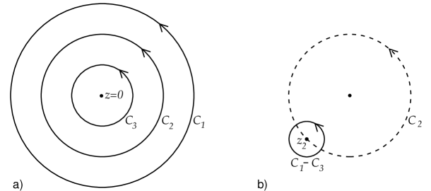
Figure 1: a) Contours centered on $z=0$. b) For given $z_{2}$ on contour $C_{2}$, contour $C_{1}-C_{3}$ is contracted.

Now, for a given point $z_{2}$ on the contour $C_{2}$, we can deform the difference of the $C_{1}$ and $C_{3}$ contours as shown in fig. 1b, with the result

$$[Q_{1},Q_{2}]\{C_{2}\}=\oint_{C_{2}}\frac{dz_{2}}{2\pi i}\,{\rm Res}_{z\to z_{2}}\,j_{1}(z)j_{2}(z_{2})$$ (1.4.5)

Applying this to the Virasoro generators gives the Virasoro algebra,

$$[L_{m},L_{n}]=(m-n)L_{m+n}+\frac{c}{12}(m^{3}-m)\delta_{m+n,0}.$$ (1.4.6)

The $\tilde{L}_{m}$ satisfy the same algebra with central charge $\tilde{c}$. For the Laurent coefficients of an analytic tensor field ${\cal O}$ of weight $(h,0)$, one finds from the OPE (1.3.13) the commutator

$$[L_{m},{\cal O}_{n}]=([h-1]m-n){\cal O}_{m+n}.$$ (1.4.7)

Note that commutation with $L_{0}$ is diagonal and proportional to $-n$. Modes ${\cal O}_{n}$ for $n>0$ reduce $L_{0}$ and are termed lowering operators, while modes ${\cal O}_{n}$ for $n<0$ increase $L_{0}$ and are termed raising operators. From the OPE (1.3.13) and the definitions, we see that a tensor operator is annihilated by all the lowering operators,

$$L_{n}\cdot{\cal O}=0,\quad n>0.$$ (1.4.8)

For an arbitrary operator, it follows from the OPE (1.3.11) that

$$L_{0}\cdot{\cal A}=h{\cal A},\qquad\tilde{L}_{0}\cdot{\cal A}=\tilde{h}{\cal A},\qquad L_{-1}\cdot{\cal A}=\partial{\cal A},\qquad\tilde{L}_{-1}\cdot{\cal A}=\bar{\partial}{\cal A}.$$ (1.4.9)

Note that $L_{0}+\tilde{L}_{0}$ is the generator of scale transformations, or in other words of radial time translations. It differs from the Hamiltonian $H$ of the cylindrical $w$ coordinate system by an additive constant from the non-tensor behavior of $T$,

$$H=L_{0}+\tilde{L}_{0}-\frac{c+\tilde{c}}{24}.$$ (1.4.10)

Similarly, $L_{0}-\tilde{L}_{0}$ measures the spin, and is equal to the spatial translation generator in the $w$ frame, up to an additive constant.

For the free $X$ CFT, the Noether current of translations is $(i\partial X(z),i\bar{\partial}X(\bar{z}))$. Again, the components are separately analytic and antianalytic, which signifies the existence of an enlarged symmetry $X\to X+y(z)+\bar{y}(\bar{z})$. Define the modes

$$i\partial X(z)=\sum_{m=-\infty}^{\infty}\frac{\alpha_{m}}{z^{m+1}},\qquad i\bar{\partial}X(\bar{z})=\sum_{m=-\infty}^{\infty}\frac{\tilde{\alpha}_{m}}{\bar{z}^{m+1}}.$$ (1.4.11)

From the OPE

$$i\partial X(z)\,i\partial X(0)=\frac{1}{z^{2}}+{\rm analytic},$$ (1.4.12)

we have the algebra

$$[\alpha_{m},\alpha_{n}]=m\delta_{m+n,0},$$ (1.4.13)

and the same for $\tilde{\alpha}_{m}$. As expected for a free field, this is a harmonic oscillator algebra for each mode; in terms of the usual raising and lowering operators $\alpha_{m}\sim\sqrt{m}a$, $\alpha_{-m}\sim\sqrt{m}a^{\dagger}$. To generate the whole spectrum we start from a state $|0,k\rangle$ which is annihilated by the $m>0$ operators and is an eigenvector of the $m=0$ operators,

$$\alpha_{m}|0,k\rangle=\tilde{\alpha}_{m}|0,k\rangle=0,\ \ m>0,\qquad\alpha_{0}|0,k\rangle=\tilde{\alpha}_{0}|0,k\rangle=k|0,k\rangle\ .$$ (1.4.14)

The rest of the spectrum is generated by the raising operators $\alpha_{m}$ and $\tilde{\alpha}_{m}$ for $m<0$. Note that the eigenvalues of $\alpha_{0}$ and $\tilde{\alpha}_{0}$ must be equal because $X$ is single valued, $\oint(dz\,\partial X+d\bar{z}\,\bar{\partial}X)=0$; later we will relax this.

Inserting the expansion (1.4.11) into $T(z)$ and comparing with the Laurent expansion gives

$$L_{m}\sim\frac{1}{2}\sum_{n=-\infty}^{\infty}\alpha_{n}\alpha_{m-n}.$$ (1.4.15)

However, we must be careful about operator ordering. The Virasoro generators were defined in terms of the normal ordering (1.1.12), while for the mode expansion it is most convenient to use a different ordering, in which all raising operators are to the left of the lowering operators. Both of these procedures are generally referred to as normal ordering, but they are in general different, so we might refer to the first as ‘conformal normal ordering’ and the latter as ‘creation-annihilation normal ordering.’ Since conformal normal order is our usual method, we will simply refer to it as normal ordering. We could develop a dictionary between these, but there are several ways to take a short-cut. Only for $m=0$ do non-commuting operators appear together, so we must have

$$L_{0} = \frac{1}{2}\alpha_{0}^{2}+\sum_{n=1}^{\infty}\alpha_{-n}\alpha_{n}+A$$

$$L_{m} = \frac{1}{2}\sum_{n=-\infty}^{\infty}\alpha_{n}\alpha_{m-n},\qquad m\neq 0.$$ (1.4.16)

for some constant $A$. Now use the Virasoro algebra as follows

$$(L_{1}L_{-1}-L_{-1}L_{1})|0,0\rangle\ =\ 2L_{0}|0,0\rangle\ =\ 2A|0,0\rangle.$$ (1.4.17)

All terms on the left have $\alpha_{m}$ with $m\geq 0$ acting on $|0,0\rangle$ and so must vanish; thus,

$$A=0.$$ (1.4.18)

Thus, a general state

$$\alpha_{-m_{1}}\ldots\alpha_{-m_{p}}\tilde{\alpha}_{-m^{\prime}_{1}}\ldots\tilde{\alpha}_{-m^{\prime}_{q}}|0,k\rangle$$ (1.4.19)

has

$$L_{0}=\frac{1}{2}k^{2}+{\sf L},\qquad\tilde{L}_{0}=\frac{1}{2}k^{2}+{\sf\tilde{L}}$$ (1.4.20)

where the levels ${\sf L}$, ${\sf\tilde{L}}$ are the total oscillator excitation numbers,

$${\sf L}=m_{1}+\ldots+m_{p},\qquad{\sf\tilde{L}}=m^{\prime}_{1}+\ldots+m^{\prime}_{q}.$$ (1.4.21)

One needs to calculate the normal ordering constant $A$ often, so the following heuristic-but-correct rules are useful:
1. Add the zero point energies, $\frac{1}{2}\omega$ for each bosonic mode and $-\frac{1}{2}\omega$ for each fermionic.
2. One encounters divergent sums of the form $\sum_{n=1}^{\infty}(n-\theta)$, the $\theta$ arising when one considers nontrivial periodicity conditions. Define this to be

$$\sum_{n=1}^{\infty}(n-\theta)=\frac{1}{24}-\frac{1}{8}(2\theta-1)^{2}.$$ (1.4.22)

I will not try to justify this, but it is the value given by any conformally invariant renormalization.
3. The above is correct in the cylindrical $w$ coordinate, but for $L_{0}$ we must add the non-tensor correction $c/24$.
For the free boson, the modes are integer so we get one-half of the sum (1.4.22) for $\theta=0$, that is $-\frac{1}{24}$, after step 2. This is just offset by the correction in step 3. The zero-point sum in step 2 is a Casimir energy, from the finite spatial size. For a system of physical size $l$ we must scale $H$ by $2\pi/l$, giving (including the left-movers) the correct Casimir energy $-\pi/6l$. For antiperiodic scalars one gets the sum with $\theta=\frac{1}{2}$ and Casimir energy $\pi/12l$.

To get the mode expansion for $X$, integrate the Laurent expansions (1.4.11). Define first

$$X_{L}(z)=x_{L}-i\alpha_{0}\ln z+i\sum_{m\neq 0}\frac{\alpha_{m}}{mz^{m}},\qquad X_{R}(\bar{z})=x_{R}-i\tilde{\alpha}_{0}\ln\bar{z}+i\sum_{m\neq 0}\frac{\tilde{\alpha}_{m}}{m\bar{z}^{m}},$$ (1.4.23)

with

$$[x_{L},\alpha_{0}]=[x_{R},\tilde{\alpha}_{0}]=i.$$ (1.4.24)

These give

$$X_{L}(z)X_{L}(z^{\prime})=-\ln(z-z^{\prime})+{\rm analytic},\qquad X_{R}(\bar{z})X_{R}(\bar{z}^{\prime})=-\ln(\bar{z}-\bar{z}^{\prime})+{\rm analytic}.$$ (1.4.25)

Actually, these only hold modulo $i\pi$ as one can check, but we will not dwell on this. In any case we are for the present only interested in the sum,

$$X(z,\bar{z})=X_{L}(z)+X_{R}(\bar{z}),$$ (1.4.26)

for which the OPE $X(z,\bar{z})X(0,0)\sim-\ln|z|^{2}$ is unambiguous.

1.5 States and Operators

Radial quantization gives rise to a natural isomorphism between the state space of the CFT, in a periodic spatial dimension, and the space of local operators. Consider the path integral with a local operator ${\cal A}$ at the origin, no other operators inside the unit circle $|z|=1$, and unspecified operators and boundary conditions outside. Cutting open the path integral on the unit circle represents the path integral as an inner product $\langle\psi_{\rm out}|\psi_{\rm in}\rangle$, where $|\psi_{\rm in}\rangle$ is the incoming state produced by the path integral at $|z|<1$ and $|\psi_{\rm out}\rangle$ is the outgoing state produced by the path integral at $|z|>1$. More explicitly, separate the path integral over fields $\phi$ into an integral over the fields outside the circle, inside the circle, and on the circle itself; call these last $\phi_{B}$. The outside integral produces a result $\psi_{\rm out}(\phi_{B})$, and the inside integral a result $\psi_{\rm in}(\phi_{B})$, leaving

$$\int[d\phi_{B}]\,\psi_{\rm out}(\phi_{B})\psi_{\rm in}(\phi_{B})\ .$$ (1.5.1)

The incoming state depends on $\cal A$, so we denote it more explicitly as $|\psi_{\cal A}\rangle$. This is the mapping from operators to states. That is, integrating over the fields on the unit disk, with fixed boundary values $\phi_{B}$ and with an operator $\cal A$ at the origin, produces a result $\psi_{\cal A}(\phi_{B})$, which is a state in the Schrodinger representation. The mapping from operators to states is given by the path integral on the unit disk. To see the inverse, take a state $|\psi\rangle$ to be an eigenstate of $L_{0}$ and $\tilde{L}_{0}$. Since $L_{0}+\tilde{L}_{0}$ is the radial Hamiltonian, inserting $|\psi\rangle$ on the unit circle is equivalent to inserting $r^{-L_{0}-\tilde{L}_{0}}|\psi\rangle$ on a circle of radius $r$. Taking $r$ to be infinitesimal defines a local operator which is equivalent to $|\psi\rangle$ on the unit circle.
Exercise: This all sounds a bit abstract, so here is a calculation one can do explicitly. The ground state of the free scalar is $e^{-\sum_{m=1}^{\infty}mX_{m}X_{-m}/2}$, where $X_{m}$ are the Fourier modes of $X$ on the circle. Derive this by canonical quantization of the modes, writing them in terms of $X_{m}$ and $\partial/\partial X_{m}$. Obtain it also by evaluating the path integral on the unit disk with $X$ fixed on the boundary and no operator insertions. Thus the ground state corresponds to the unit operator.

Usually one does not actually evaluate a path integral as above, but uses indirect arguments. Note that if $Q$ is any conserved charge, the state $Q|\psi_{\cal A}\rangle$ corresponds to the operator $Q\cdot{\cal A}$, as shown in fig. 2.

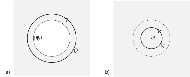
Figure 2: a) World-sheet (shaded) with state $|\psi_{\cal A}\rangle$ on the boundary circle, acted upon by $Q$. b) Equivalent picture: the unit disk with operator ${\cal A}$ has been sewn in along the dotted line, and $Q$ contracted around the operator.

Now, in the free theory consider the case that ${\cal A}$ is the unit operator and let

$$Q=\alpha_{m}=\oint_{C}\frac{dz}{2\pi}z^{m}\partial X,\qquad m\geq 0.$$ (1.5.2)

With no operators inside the disk, $\partial X$ is analytic and the integral vanishes for $m\geq 0$. Thus, $\alpha_{m}|\psi_{1}\rangle=0$, $m\geq 0$, which establishes

$$1\ \leftrightarrow\ |0,0\rangle$$ (1.5.3)

as found directly in the exercise. Proceeding as above one finds

$$:\!e^{ikX}\!:\ \leftrightarrow\ |0,k\rangle,$$ (1.5.4)

and for the raising operators, evaluating the contour integral (1.5.2) for $m<0$ gives

$$i\frac{1}{(k-1)!}\partial^{k}X\ \leftrightarrow\ \alpha_{-k},\quad k\geq 1\ ,$$ (1.5.5)

and in parallel for the tilded modes. That is, the state obtained by acting with raising operators on (1.5.4) is given by the product of the exponential with the corresponding derivatives of $X$; the product automatically comes out normal ordered.

The state corresponding to a tensor field ${\cal O}$ satisfies

$$L_{m}|\psi_{\cal O}\rangle=0,\qquad m>0.$$ (1.5.6)

This is known as a highest weight or primary state. For almost all purposes one is interested in highest-weight representations of the Virasoro algebra, built by acting on a given highest weight state with the $L_{m}$, $m<0$.

The state-operator mapping gives a simple derivation of the OPE, shown in fig. 3.

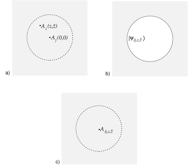
Figure 3: a) World-sheet with two local operators. b) Integration over fields on the interior of the disk produces boundary state $|\psi_{ij,z,\bar{z}}\rangle$. c) Sewing in a disk with the corresponding local operator. Expanding in operators of definite weight gives the OPE.

Consider the product ${\cal A}_{i}(z,\bar{z}){\cal A}_{j}(0,0)$, $|z|<1$. Integrating the fields inside the unit circle generates a state on the unit circle, which we might call $|\psi_{ij,z,\bar{z}}\rangle$. Expand in a complete set,

$$|\psi_{ij,z,\bar{z}}\rangle=\sum_{k}c^{k}\!_{ij}(z,\bar{z})|\psi_{k}\rangle.$$ (1.5.7)

Finally use the mapping to replace $|\psi_{k}\rangle$ on the unit circle with ${\cal A}_{k}$ at the origin, giving the general OPE (1.1.15). The claimed convergence is just the usual convergence of a complete set in quantum mechanics. The construction is possible as long as there are no other operators with $|z^{\prime}|\leq|z|$, so that we can cut on a circle of radius $|z|+\epsilon$.

Incidentally, applying a rigid rotation and scaling to both sides of the general OPE determines the $z$-dependence of the coefficient functions,

$${\cal A}_{i}(z,\bar{z}){\cal A}_{j}(0,0)=\sum_{k}z^{h_{k}-h_{i}-h_{j}}{\bar{z}}^{\tilde{h}_{k}-\tilde{h}_{i}-\tilde{h}_{j}}c^{k}\!_{ij}{\cal A}_{k}(0,0).$$ (1.5.8)

From the full conformal symmetry one learns much more: all the $c^{k}\!_{ij}$ are determined in terms of those of the primary fields.

For three operators, ${\cal A}_{i}(0){\cal A}_{j}(1){\cal A}_{k}(z)$, the regions of convergence of the $z\to 0$ and $z\to 1$ OPE’s ($|z|<1$ and $|1-z|<1$) overlap. The coefficient of ${\cal A}_{m}$ in the triple product can then be written as a sum involving $c^{l}\!_{ik}c^{m}\!_{lj}$ or as a sum involving $c^{l}\!_{jk}c^{m}\!_{li}$. Associativity requires these sums to be equal; this is represented schematically in fig. 4.

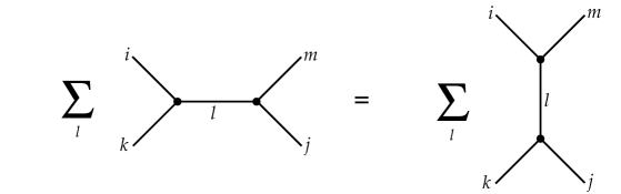
Figure 4: Schematic picture of OPE associativity.

A unitary CFT is one that has a positive inner product $\langle\!\langle\ |\ \rangle$; the double bracket is to distinguish it from a different inner product to be defined later. Also, it is required that $L_{m}^{\dagger}=L_{-m}$, $\tilde{L}_{m}^{\dagger}=\tilde{L}_{-m}$. The $X$ CFT is unitary with

$$\langle\!\langle 0,k|0,k^{\prime}\rangle=2\pi\delta(k-k^{\prime})$$ (1.5.9)

and $\alpha_{m}^{\dagger}=\alpha_{-m}$, $\tilde{\alpha}_{m}^{\dagger}=\tilde{\alpha}_{-m}$; this implicitly defines the inner product of all higher states. Unitary CFT’s are highly constrained; I will derive here a few of the basic results, and mention others later.

The first constraint is that any state in a unitary highest weight representation must have $h,\tilde{h}\geq 0$. Consider first the highest weight state itself, $|{\cal O}\rangle$. The Virasoro algebra gives

$$2h_{\cal O}\langle\!\langle{\cal O}|{\cal O}\rangle=2\langle\!\langle{\cal O}|L_{0}|{\cal O}\rangle=\langle\!\langle{\cal O}|[L_{1},L_{-1}]|{\cal O}\rangle=\|L_{-1}|{\cal O}\rangle\|^{2}\geq 0,$$ (1.5.10)

so $h_{\cal O}\geq 0$. All other states in the representation, obtained by acting with the raising generators, have higher weight so the result follows. It also follows that if $h_{\cal O}=0$ then $L_{-1}\cdot{\cal O}=\tilde{L}_{-1}\cdot{\cal O}$. The relation (1.4.9) thus implies that $\cal O$ is independent of position; general principle of quantum field theory then require $\cal O$ to be a $c$-number. That is, the unit operator is the only (0,0) operator. In a similar way, one finds that an operator in a unitary CFT is analytic if and only if $\tilde{h}=0$, and antianalytic if and only if $h=0$.
Exercise: Using the above argument with the commutator $[L_{n},L_{-n}]$, show that $c,\tilde{c}\geq 0$ in a unitary CFT. In fact, the only CFT with $c=0$ is the trivial one, $L_{n}=0$.

1.6 Other CFT’s

Now we describe briefly several other CFT’s of interest. The first is given by the same action (1.1.7) as the earlier $X$ theory, but with energy-momentum tensor [22]

$$T(z)=-\frac{1}{2}:\!\partial X\partial X\!:+\,\frac{Q}{2}\partial^{2}X,\qquad\tilde{T}(\bar{z})=-\frac{1}{2}:\!\bar{\partial}X\bar{\partial}X\!:+\,\frac{Q}{2}\bar{\partial}^{2}X.$$ (1.6.1)

The $TT$ operator product is still of the general form (1.3.16), but now has central charge $c=1+3Q^{2}$. The change in $T$ means that $X$ is no longer a scalar,

$$\delta X=-(g\partial X+\bar{g}\bar{\partial}X)-\frac{Q}{2}(\partial g+\bar{\partial}\bar{g}).$$ (1.6.2)

Exponentials $:\!e^{ikX}\!:$ are still tensors, but with weight $\frac{1}{2}(k^{2}+ikQ)$. One notable change is in the state-operator mapping. The translation current $j=i\partial X$ is no longer a tensor, $\delta j=-g\partial j-j\partial g-iQ\partial^{2}g/2$. The finite form is

$$(\partial_{z}z^{\prime})j_{z^{\prime}}(z^{\prime})=j_{z}(z)-\frac{iQ}{2}\frac{\partial^{2}_{z}z^{\prime}}{\partial_{z}z^{\prime}}.$$ (1.6.3)

Applied to the cylinder frame $z^{\prime}=w=i\ln z$ this gives

$$\frac{1}{2\pi i}\int dw\,j_{w}=\alpha_{0}+\frac{iQ}{2}.$$ (1.6.4)

Thus a state $|0,k\rangle$ which whose canonical momentum (defined on the left) is $k$ corresponds to the operator

$$:\!e^{ikX+QX/2}\!:\ .$$ (1.6.5)

Note that $i\alpha_{0}$ just picks out the exponent of the operator, so $\alpha_{0}=k-iQ/2$.

The mode expansion of the $m\neq 0$ generators is

$$L_{m}=\frac{1}{2}\sum_{n=-\infty}^{\infty}\alpha_{n}\alpha_{m-n}+\frac{iQ}{2}(m+1)\alpha_{m},\qquad m\neq 0,$$ (1.6.6)

the last term coming from the $\partial^{2}X$ term in $T$. For $m=0$ the result is

$$L_{0} = \frac{1}{8}(2\alpha_{0}+iQ)^{2}+\frac{Q^{2}}{8}+\sum_{n=1}^{\infty}\alpha^{\mu}_{-n}\alpha_{\mu,n}$$ (1.6.7)

$$= \frac{1}{2}k^{2}+\frac{Q^{2}}{8}+\sum_{n=1}^{\infty}\alpha^{\mu}_{-n}\alpha_{\mu,n}.$$

The constant in the first line can be obtained from the $z^{-2}$ term in the OPE of $T$ with the vertex operator (1.6.5); this is a quick way to derive or to check normal-ordering constants. In the second line, expressed in terms of the ‘canonical’ momentum $k$ it agrees with our heuristic rules.

This CFT has a number of applications in string theory, some of which we will encounter. Let me also mention a slight variation,

$$T(z)=-\frac{1}{2}:\!\partial X\partial X\!:+\,i\frac{\kappa}{2}\partial^{2}X,\qquad\tilde{T}(\bar{z})=-\frac{1}{2}:\!\bar{\partial}X\bar{\partial}X\!:-\,i\frac{\kappa}{2}\bar{\partial}^{2}X,$$ (1.6.8)

with central charge $c=1-3\kappa^{2}$. With the earlier transformation (1.6.2), the variation of $X$ contains a constant piece under rigid scale transformations ($g$ a real constant). In other words, one can regard $X$ as the Goldstone boson of spontaneously broken scale invariance. For the theory (1.6.8), the variation of $X$ contains a constant piece under rigid rotations ($g$ an imaginary constant), and $X$ is the Goldstone boson of spontaneously broken rotational invariance. This is not directly relevant to string theory (the $i$ in the energy-momentum tensor makes the theory non-unitary) but occurs for real membranes (where the unitarity condition is not relevant because both dimensions are spatial). In particular the CFT (1.6.8) describes hexatic membranes, in which the rotational symmetry is broken to ${\bf Z}_{6}$. The unbroken discrete symmetry plays an indirect role in forbidding certain nonlinear couplings between the Goldstone boson $X$ and the membrane coordinates.

Another simple variation on the free boson is to make it periodic, but we leave this until section 3 where we will discuss some interesting features.

Another family of free CFT’s involves two anticommuting fields with action

$$S=\frac{1}{2\pi}\int d^{2}z\,\{b\bar{\partial}c+\tilde{b}\partial\tilde{c}\}.$$ (1.6.9)

The equations of motion are

$$\bar{\partial}c(z)=\bar{\partial}b(z)=\partial\tilde{c}(\bar{z})=\partial\tilde{b}(\bar{z})=0,$$ (1.6.10)

so the fields are respectively analytic and antianalytic. The operator products are readily found as before, with appropriate attention to the order of anticommuting variables,

$$b(z)c(0)\sim\frac{1}{z},\qquad c(z)b(0)\sim\frac{1}{z},\qquad\tilde{b}(\bar{z})\tilde{c}(0)\sim\frac{1}{\bar{z}},\qquad\tilde{c}(\bar{z})\tilde{b}(0)\sim\frac{1}{\bar{z}}.$$ (1.6.11)

We focus again on the analytic part; in fact the action (1.6.9) is a sum, and can be regarded as two independent CFT’s. The action is conformally invariant if $b$ is a $(\lambda,0)$ tensor, and $c$ a $(1-\lambda,0)$ tensor; by interchange of $b$ and $c$ we can assume $\lambda$ positive. The corresponding energy-momentum tensor is

$$T(z)=:\!(\partial b)c\!:-\lambda:\!\partial(bc)\!:\ .$$ (1.6.12)

One finds that the $TT$ OPE has the usual form with

$$c=-3(2\lambda-1)^{2}+1.$$ (1.6.13)

The fields have the usual Laurent expansions

$$b(z)=\sum_{m=-\infty}^{\infty}\frac{b_{m}}{z^{m+\lambda}},\qquad c(z)=\sum_{m=-\infty}^{\infty}\frac{c_{m}}{z^{m+1-\lambda}},$$ (1.6.14)

giving rise to the anticommutator

$$\{b_{m},c_{n}\}=\delta_{m+n,0}.$$ (1.6.15)

Also, $\{c_{m},c_{n}\}=\{b_{m},b_{n}\}=0$. Because of the $m=0$ modes there are two natural ground states, $|\!\uparrow\rangle$ and $|\!\downarrow\rangle$. Both are annihilated by $b_{m}$ and $c_{m}$ for $m>0$, while

$$b_{0}|\!\downarrow\rangle=0,\qquad c_{0}|\!\uparrow\rangle=0.$$ (1.6.16)

These are related $|\!\uparrow\rangle=c_{0}|\!\downarrow\rangle$, $|\!\downarrow\rangle=b_{0}|\!\uparrow\rangle$. With the antianalytic theory included, there are also the zero modes $\tilde{b}_{0}$ and $\tilde{c}_{0}$ and so four ground states—$|\!\downarrow\downarrow\rangle$, etc.

The Virasoro generators in terms of the modes are

$$L_{0} = \sum_{n=1}^{\infty}n(b_{-n}c_{n}+c_{-n}b_{n})\ -\ \frac{\lambda(\lambda-1)}{2}$$

$$L_{m} = \sum_{n=-\infty}^{\infty}\{\lambda m-n\}b_{n}c_{m-n},\quad m\neq 0\ .$$ (1.6.17)

The ordering constant is found as before. Two sets ($b$ and $c$) of integer anticommuting modes give $\frac{1}{12}$ at step 2, and the central charge correction then gives the result above.

The state-operator mapping is a little tricky. Let $\lambda$ be an integer, so that the Laurent expansion (1.6.14) has no branch cut. For the unit operator the fields are analytic at the origin, so

$$b_{m}|\psi_{1}\rangle=0,\quad m\geq 1-\lambda,\qquad c_{m}|\psi_{1}\rangle=0,\quad m\geq\lambda.$$ (1.6.18)

Thus, the unit state is in general not one of the ground states, but rather

$$|\psi_{1}\rangle=b_{-1}b_{-2}\ldots b_{1-\lambda}|\!\downarrow\rangle,$$ (1.6.19)

up to normalization. Also, we have the dictionary

$$b_{-m}\ \leftrightarrow\ \frac{1}{(m-\lambda)!}\partial^{m-\lambda}b,\qquad c_{-m}\ \leftrightarrow\ \frac{1}{(m+\lambda-1)!}\partial^{m+\lambda-1}c.$$ (1.6.20)

Thus we have, taking the value $\lambda=2$ which will be relevant later,

$$|\!\downarrow\rangle=c_{1}|\psi_{1}\rangle\ \leftrightarrow\ c,\qquad|\!\uparrow\rangle=c_{0}c_{1}|\psi_{1}\rangle\ \leftrightarrow\ \partial c\,c.$$ (1.6.21)

The $bc$ theory has a conserved current $j=\ :\!cb\!:$, called ghost number, which counts the number of $c$’s minus the number of $b$’s. In the cylindrical $w$ frame the vacua have average ghost number zero, so $-\frac{1}{2}$ for $|\!\downarrow\rangle$ and $+\frac{1}{2}$ for $|\!\uparrow\rangle$. The ghost numbers of the corresponding operators are $\lambda-1$ and $\lambda$, as we see from the example (1.6.21). As in the case of the momentum (1.6.4), the difference arises because the current is not a tensor.

For the special case $\lambda=\frac{1}{2}$, $b$ and $c$ have the same weight and the $bc$ system can be split in two in a conformally invariant way, $b=(\psi_{1}+i\psi_{2})/\sqrt{2}$, $c=(\psi_{1}-i\psi_{2})/\sqrt{2}$, and

$$S=\frac{1}{2\pi}\int d^{2}z\,b\bar{\partial}c=\frac{1}{4\pi}\int d^{2}z\,\Bigl{\{}\psi_{1}\bar{\partial}\psi_{1}+\psi_{2}\bar{\partial}\psi_{2}\Bigr{\}}.$$ (1.6.22)

Each $\psi$ theory has central charge $\frac{1}{2}$. The antianalytic theory separates in the same way. We will refer to these as Majorana (real) fermions, because it is a unitary CFT with $\psi_{m}^{\dagger}=\psi_{-m}$.

Another family of CFT’s differs from the $bc$ system only in that the fields commute. The action is

$$S=\frac{1}{2\pi}\int d^{2}z\,\beta\bar{\partial}\gamma\ .$$ (1.6.23)

The fields $\beta$ and $\gamma$ are analytic by the equations of motion; as usual there is a corresponding antianalytic theory. Because the statistics are changed, some signs in operator products are different,

$$\beta(z)\gamma(0)\sim-\frac{1}{z},\qquad\gamma(z)\beta(0)\sim\frac{1}{z}.$$ (1.6.24)

The action is conformally invariant with $\beta$ a weight $(\lambda,0)$ tensor and $\gamma$ a $(1-\lambda,0)$ tensor. The energy-momentum tensor is

$$T(z)=\ :\!(\partial\beta)\gamma\!:-\lambda:\!\partial(\beta\gamma)\!:\ .$$ (1.6.25)

The central charge has the opposite sign relative to the $bc$ system because of the changed statistics,

$$c=3(2\lambda-1)^{2}-1.$$ (1.6.26)

All of the above are free field theories. A simple interacting theory is the non-linear sigma model [23]-[25], consisting of $D$ scalars $X^{\mu}$ with a field-dependent kinetic term,

$$S=\frac{1}{4\pi}\int d^{2}z\,\Bigr{\{}G_{\mu\nu}(X)+iB_{\mu\nu}(X)\Bigl{\}}\partial X^{\mu}\bar{\partial}X^{\nu},$$ (1.6.27)

with $G_{\mu\nu}=G_{\nu\mu}$ and $B_{\mu\nu}=-B_{\nu\mu}$. Effectively the scalars define a curved field space, with $G_{\mu\nu}$ the metric on the space. The path integral is no longer gaussian, but when $G_{\mu\nu}(X)$ and $B_{\mu\nu}(X)$ are slowly varying the interactions are weak and there is a small parameter. The action is naively conformally invariant, but a one-loop calculation reveals an anomaly (obviously this is closely related to the $\beta$-function for rigid scale transformations),

$$T_{z\bar{z}}=\biggr{\{}-2{\bf R}_{\mu\nu}+\frac{1}{2}H_{\mu\sigma\rho}H_{\nu}\!^{\sigma\rho}+\nabla^{\sigma}H_{\sigma\mu\nu}\biggr{\}}\partial X^{\mu}\bar{\partial}X^{\nu}\ .$$ (1.6.28)

Here ${\bf R}_{\mu\nu}$ is the Ricci curvature built from $G_{\mu\nu}$ (I am using boldface to distinguish it from the two-dimensional curvature to appear later), $\nabla^{\sigma}$ denotes the covariant derivative in this metric, and

$$H_{\sigma\mu\nu}=\partial_{\sigma}B_{\mu\nu}+\partial_{\mu}B_{\nu\sigma}+\partial_{\nu}B_{\sigma\mu}.$$ (1.6.29)

To this order, any Ricci-flat space with $B_{\mu\nu}=0$ gives a CFT. At higher order these conditions receive corrections. Other solutions involve cancellations between terms in (1.6.28). A three dimensional example is the 3-sphere with a round metric of radius $r$, and with

$$H_{\sigma\mu\nu}=\frac{4q}{r^{3}}\epsilon_{\sigma\mu\nu}$$ (1.6.30)

proportional to the antisymmetric three-tensor. By symmetry, the first two terms in $T_{z\bar{z}}$ are proportional to $G_{\mu\nu}\partial X^{\mu}\bar{\partial}X^{\nu}$ and the third vanishes. Thus $T_{z\bar{z}}$ vanishes for an appropriate relation between the constants, $r^{4}=4q^{2}$. There is one subtlety. Locally the form (1.6.30) is compatible with the definition (1.6.29) but not globally. This configuration is the analog of a magnetic monopole, with the gauge potential $B_{\mu\nu}$ now having two indices and the field strength $H_{\sigma\mu\nu}$. Then $B_{\mu\nu}$ must have a ‘Dirac string’ singularity, which is invisible to the string if the field strength is appropriately quantized; I have normalized $q$ just such that it must be an integer. So this defines a discrete series of models. The one-loop correction to the central charge is $c=3-6/|q|+O(1/q^{2})$. The 3-sphere is the $SU(2)$ group space, and the theory just described is the $SU(2)$ Wess-Zumino-Witten (WZW) model [26]-[28] at level $q$. It can be generalized to any Lie group. Although this discussion is based on the one-loop approximation, which is accurate for large $r$ (small gradients) and so for large $q$, these models can also be constructed exactly, as will be discussed further shortly.

For $c<1$, it can be shown that unitary CFT’s can exist only at the special values [19], [29]

$$c=1-\frac{6}{m(m+1)},\qquad m=2,3,\ldots.$$ (1.6.31)

These are the unitary minimal models, and can be solved using conformal symmetry alone. The point is that for $c<1$ the representations are all degenerate, certain linear combinations of raising operators annihilating the highest weight state, which gives rise to differential equations for the expectation value of the corresponding tensor operator. These CFT’s have a $Z_{2}$ symmetry and $m-2$ relevant operators, and correspond to interesting critical systems: $m=3$ to the Ising model (note that $c=\frac{1}{2}$ corresponds to the free fermion), $m=4$ to the tricritical Ising model, $m=5$ to a multicritical $Z_{2}$ Ising model but also to the three-state Potts model, and so on.

This gives a survey of the main categories of conformal field theory, including some CFT’s that will be of specific interest to us later on. It is familiar that there are many equivalences between different two dimensional field theories. For example, the ordinary free boson is equivalent to a free fermion, which is the same as the $bc$ system at $\lambda=\frac{1}{2}$. The bosonization dictionary is

$$b\equiv\ :\!e^{iX}\!:\ ,\qquad c\equiv\ :\!e^{-iX}\!:\$$ (1.6.32)

In fact this extends to the general $bc$ and $X$ CFT’s, with complex $Q=i(1-2\lambda)$. The reader can check that the weights of $b$ and $c$, and the central charge, then match. There is also a rewriting of $\beta$ and $\gamma$ in terms of exponentials, which is more complicated but useful in the superstring. All of these subjects are covered in ref. [20]. As a further example, the level 1 $SU(2)$ WZW model, which we have described in terms of three bosons, can also be written in terms of a single free boson; the level 2 $SU(2)$ WZW model can be written in terms of three Majorana fermions; these will be explained further in the next section. The minimal models are related to the free $X$ theory with $Q$ such as to give the appropriate central charge [30], but this is somewhat indirect.

1.7 Other Algebras

The Virasoro algebra is just one of several important infinite dimensional algebras. Another is obtained from $T(z)$ plus any number of analytic $(1,0)$ tensors $j^{a}(z)$. The constraints obtained at the end of section 1.5 imply that if the algebra is to have unitary representations the $jj$ OPE can only take the form

$$j^{a}(z)j^{b}(0)\sim\frac{k^{ab}}{z^{2}}+i\frac{f^{ab}\!_{c}}{z}j^{c}(0).$$ (1.7.1)

The corresponding Laurent expansion is

$$j^{a}(z)=\sum_{m=-\infty}^{\infty}\frac{j^{a}_{m}}{z^{m+1}},$$ (1.7.2)

and the corresponding algebra

$$[j^{a}_{m},j^{b}_{n}]=mk^{ab}\delta_{m+n,0}+if^{ab}\!_{c}j^{c}_{m+n}.$$ (1.7.3)

This is known variously as a current algebra, an affine Lie algebra, or sometimes as a Kac-Moody algebra; for general references see [31], [27] and [28]. The $m=n=0$ modes form an ordinary Lie algebra $g$ with structure constants $f^{ab}\!_{c}$. The latter must therefore satisfy the Jacobi identity; another Jacobi identity implies that $k^{ab}$ is $g$-invariant. The energy-momentum tensor can be shown to separate into a piece built from the current (the Sugawara construction) and a piece commuting with the current. The CFT is thus a product of a part determined by the symmetry and a part independent of the symmetry.

For a single Abelian current we already have the example of the free $X$ theory. The next simplest case is $SU(2)$,

$$[j^{a}_{m},j^{b}_{n}]=mk\delta^{ab}\delta_{m+n,0}+i\sqrt{2}\epsilon^{abc}j^{c}_{m+n}.$$ (1.7.4)

The value of $k$ must be an integer, and non-negative in a unitary theory.
Exercise: Construct an $SU(2)$ algebra containing $(j^{1}+ij^{2})_{1}$ and $(j^{1}-ij^{2})_{-1}$, and use it to show that $k$ is an integer.
The Sugawara central charge is $c=3k/(k+2)$. The $SU(2)$ WZW model just discussed has $k=|q|$. The case $k=1$ can also be realized in terms of a single free scalar as

$$j^{1}=\sqrt{2}:\!\cos\sqrt{2}X\!:\ ,\qquad j^{2}=-\sqrt{2}:\!\sin\sqrt{2}X\!:\ ,\qquad j^{3}=i\partial X\ .$$ (1.7.5)

The case $k=2$ can also be realized in terms of three Majorana fermions, $j^{a}=i\epsilon^{abc}\psi^{b}\psi^{c}/\sqrt{2}$.

The energy momentum tensor together with a weight $(\frac{3}{2},0)$ tensor current (supercurrent) $T_{F}$ form the $N=1$ superconformal algebra [32], [33]. The $T_{F}T_{F}$ OPE is

$$T_{F}(z)T_{F}(0)\sim\frac{2c}{3z^{3}}+\frac{2}{z}T(0);$$ (1.7.6)

$TT_{F}$ has the usual tensor form (1.3.13). A simple realization is in terms of a free scalar $X$ and a Majorana fermion $\psi$,

$$T_{F}=iX\partial\psi,\qquad T=-\frac{1}{2}(:\!\partial X\partial X\!:+:\!\psi\partial\psi\!:\ ).$$ (1.7.7)

With the Laurent expansions

$$T_{F}(z)=\sum_{r=-\infty}^{\infty}\frac{G_{r}}{z^{r+3/2}},\qquad\psi(z)=\sum_{r=-\infty}^{\infty}\frac{\psi_{r}}{z^{r+1/2}},$$ (1.7.8)

the algebra is

$$\{G_{r},G_{s}\}=2L_{r+s}+\frac{c}{12}(4r^{2}-1)\delta_{r+s,0}\ .$$ (1.7.9)

The central charge must be the same is in the $TT$ OPE, by the Jacobi identity. Note that for $r$ running over integers, the fields (1.7.8) have branch cuts at the origin, but the corresponding fields in the cylindrical $w$ frame are periodic due to the tensor transformation $(\partial w/\partial z)^{h}$. This is the Ramond sector. Antiperiodic boundary conditions on $\psi$ and $T_{F}$ in the $w$ frame are also possible; this is the Neveu-Schwarz sector. All of the above goes through with $r$ running over integers-plus-$\frac{1}{2}$, and the fields in the $z$ frame are single valued in this sector.
Exercise: Work out the expansions of $L_{m}$ and $G_{r}$ in terms of the modes of $X$ and $\psi$. [Answer: the normal-ordering constant is $0$ in the Neveu-Schwarz sector and $\frac{1}{16}$ in the Ramond sector.]
The operators corresponding to Ramond-sector states thus produce branch cuts in the fermionic fields, and are known as spin fields. They are most easily described using bosonization. With two copies of the free representation (1.7.7), the bosonization is $(\psi^{1}\pm i\psi^{2})/\sqrt{2}=\ :\!e^{\pm iX}\!:\$. There are two Ramond ground states, which correspond to the operators $:\!e^{\pm iX/2}\!:$. Observe that this has the necessary branch cut with $\psi^{1}$, $\psi^{2}$, and also that its weight, $\frac{1}{8}=2\frac{1}{16}$, agrees with the exercise.

The energy-momentum tensor with two $(\frac{3}{2},0)$ tensors $T_{F}^{\pm}$ plus a $(1,0)$ current $j$ form the $N=2$ superconformal algebra [34]

$$T^{+}_{F}(z)T^{-}_{F}(0) \sim \frac{2c}{3z^{3}}+\frac{1}{z^{2}}j(0)+\frac{2}{z}T(0)+\frac{1}{2z}\partial j(0),$$

$$j(z)T^{\pm}_{F}(0) \sim \pm\frac{1}{z}T^{\pm}_{F}(0),$$ (1.7.10)

with $T_{F}^{+}T_{F}^{+}$ and $T_{F}^{-}T_{F}^{-}$ analytic. This can be generalized to $N$ supercurrents, leading to an algebra with weights $2,\frac{3}{2},\ldots,2-\frac{1}{2}N$. From the earlier discussion we see that there are no unitary representations for $N>4$. There is one $N=3$ algebra and two distinct $N=4$ algebras [34],[35].

These are the algebras which play a central role in string theory, but many others arise in various CFT’s. I will briefly discuss some higher-spin algebras, which have a number of interesting applications (for reviews of the various linear and nonlinear higher spin algebras see refs. [36],[37]). The free scalar action (1.1.7) actually has an enormous amount of symmetry, but let us in particular pick out

$$\delta X(z,\bar{z})=-\sum_{l=0}^{\infty}g_{l}(z)(\partial X(z))^{l+1},\qquad l=0,1,\ldots$$ (1.7.11)

The Noether currents

$$V^{l}(z)=-\frac{1}{l+2}:\!(\partial X(z))^{l+2}\!:$$ (1.7.12)

have spins $l+2$. Making the usual Laurent expansion, one finds the $w_{\infty}$ algebra

$$[V^{i}_{m},V^{j}_{n}]=\Bigl{(}[j+1]m-[i+1]n\Bigr{)}V^{i+j}_{m+n}.$$ (1.7.13)

The $l=0$ generators are just the usual Virasoro algebra. There are a number of related algebras. Adding in the $l=-1$ generators (which are just the modes of the translation current) defines the $w_{1+\infty}$ algebra. Another algebra with the same spin content as $w_{\infty}$ but a more complicated commutator is $W_{\infty}$; $w_{\infty}$ can be obtained as a limit (contraction) of $W_{\infty}$. These algebras have a simple and useful realization in terms of the classical and quantum mechanics of a particle in one dimension:

$$V^{i}_{m}\equiv\frac{1}{4}(p+x)^{i+m+1}(p-x)^{i-m+1}.$$ (1.7.14)

The Poisson bracket algebra of these is the wedge subalgebra ($m\leq i+1$) of $w_{\infty}$; the commutator algebra is the wedge subalgebra of $W_{\infty}$. In the literature one must beware of differing notations and conventions.

All of these algebras have supersymmetric extensions, with generators of half-integral spins. There are also various algebras with a finite number of higher weights. One family is $W_{N}$, closely related to $W_{\infty}$, with weights up to $N$. The commutator of two weight-3 currents in $W_{\infty}$ contains the weight-4 current. In $W_{3}$ this is not an independent current but the square of $T(z)$, so the algebra is nonlinear.

1.8 Riemann Surfaces

Thus far we have focussed on local properties, without regard to the global structure or boundary conditions. For string theory we will be interested in conformal field theories on closed manifolds. The appropriate manifold for a two-dimensional CFT to live on is a two-dimensional complex manifold, a Riemann surface. One can imagine this as being built up from patches, patch $i$ having a coordinate $z^{(i)}$ which runs over some portion of the complex plane. If patches $i$ and $j$ overlap, there is a relation between the coordinates,

$$z^{(j)}=f_{ij}(z^{(i)})$$ (1.8.1)

with $f_{ij}$ an analytic function. Two Riemann surfaces are equivalent if there is a mapping between them such that the coordinates on one are analytic functions of the coordinates on the other. This is entirely parallel to the definition of a differentiable manifold, but it has more structure—the manifold comes with a local notion of analyticity. Since in a CFT each field has a specific transformation law under analytic changes of coordinates, the transition function (1.8.1) is just the information needed to extend the field from patch to patch.

A simple example is the sphere, which we can imagine as built from two copies of the complex plane, with coordinates $z$ and $u$, with the mapping

$$u=-\frac{1}{z}.$$ (1.8.2)

The $z$ coordinate cannot quite cover the sphere, the point at infinity being missing. All Riemann surfaces with the topology of the sphere are equivalent. For future reference let us note that the sphere has a group of globally defined conformal transformations (conformal Killing transformations), which in the $z$ patch take

$$z^{\prime}=\frac{\alpha z+\beta}{\gamma z+\delta},$$ (1.8.3)

where $\alpha$, $\beta$, $\gamma$ and $\delta$ are complex parameters which can be chosen such that $\alpha\delta-\beta\gamma=1$. This is the Möbius group.

The next Riemann surface is the torus. Rather than build it from patches it is most convenient to describe it as in fig. 5 by taking a single copy $z$ of the complex plane and identifying points

$$z\ \cong\ z+2\pi\ \cong\ z+2\pi\tau,$$ (1.8.4)

producing a parallelogram-shaped region with opposite edges identified.

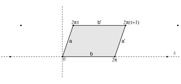
Figure 5: The torus by periodic identification of the complex plane. Points identified with the origin are indicated. Edges $a$ and $a^{\prime}$ are identified, as are edges $b$ and $b^{\prime}$.

Different values of $\tau$ in general define inequivalent Riemann surfaces; $\tau$ is known as a modulus for the complex structure on the torus. However, there are some equivalences: $\tau$, $-\tau$, $\tau+1$, and $-1/\tau$ generate the same group of transformations of the complex plane and so the same surface (to see the last of these, let $z=-z^{\prime}\tau$). So we may restrict to Im$(\tau)>0$ and moreover identify

$$\tau\sim\tau+1\sim-\frac{1}{\tau}.$$ (1.8.5)

These generate the modular group

$$\tau^{\prime}=\frac{a\tau+b}{c\tau+d},$$ (1.8.6)

where now $a$, $b$, $c$, $d$ are integers such that $ad-bc=1$. A fundamental region for this is given by $|\tau|\geq 1$, Re$(\tau)\leq\frac{1}{2}$, shown in fig. 6.

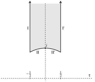
Figure 6: The standard fundamental region for the modulus $\tau$ of the torus. Identifying boundaries I and I^′, and II and II^′, produces the moduli space for the torus. Note that this is a closed space except for the limit Im$(\tau)\to\infty$.

This is the moduli space for the torus: every Riemann surface with this topology is equivalent to one with $\tau$ in this region. The torus also has a conformal Killing transformation, $z\to z+\alpha$.

Notice the similarity between the transformations (1.8.3) and (1.8.6), differing only in whether the parameters are complex numbers or integers. You can check that successive transformations compose like matrix multiplication, so these are the groups $SL(2,C)$ and $SL(2,Z)$ respectively ($2\times 2$ matrices of determinant one). We will meet $SL(2,Z)$ again in a different physical context.

Any closed oriented oriented two-dimensional surface can be obtained by adding $h$ handles to the sphere; $h$ is the genus. It is often useful to think of higher genus surfaces built up from lower via the plumbing fixture construction. This essential idea is developed in many places, but my lectures have been most influenced by the approach in refs [38]-[41]. Let $z^{(1)}$ and $z^{(2)}$ be coordinates in two patches, which may be on the same Riemann surface or on different Riemann surfaces. For complex $q$, cut out the circles $|z^{(1)}|,|z^{(2)}|<(1-\epsilon)|q|^{1/2}$ and identify points on the cut surfaces such that

$$z^{(1)}z^{(2)}=q,$$ (1.8.7)

as shown in fig. 7.

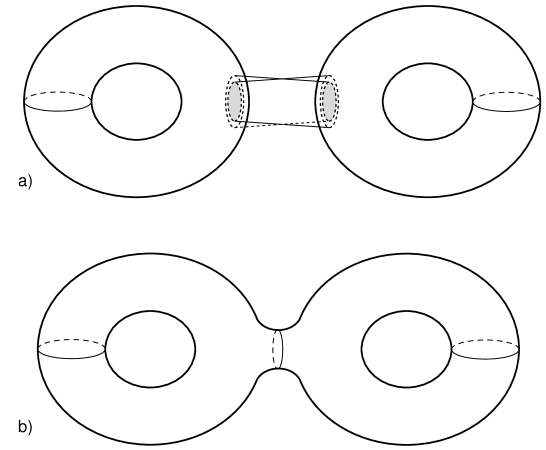
Figure 7: Plumbing fixture construction. Identifying annular regions as in (a) produces the sewn surface (b).

If $z^{(1)}$ and $z^{(2)}$ are on the same surface, this adds a handle. The genus-$h$ surface can be constructed from the sphere by applying this $h$ times. The number of complex parameters in the construction is $3h$, being $q$ and the position of each end for each handle, minus 3 from an overcounting due to the Möbius group, leaving $3h-3$ which is the correct number of complex moduli. An index theorem states that the number of complex moduli minus the number of conformal Killing transformations is $3h-3$, as we indeed have in each case.

Note that for $q<1$ the region between the circles $|z^{(1)}|=1$ and $|z^{(2)}|=1$ is conformal to the cylindrical region

$$0<{\rm Im}(w)<2\pi\ln(1/|q|),\qquad w\ \cong\ w+2\pi,$$ (1.8.8)

which becomes long in the limit $q\to 0$.

Just as conformal transformations can be described as the most general coordinate transformation which leave $dz$ invariant up to local multiplication, there is a geometric interpretation for the superconformal transformations. The $N=1$ algebra, for example, can be described in terms of a space with two ordinary and two anticommuting coordinates $(z,\bar{z},\theta,\bar{\theta})$ as the space of transformations which leave $dz+i\theta d\theta$ invariant up to local multiplication. Super-Riemann surfaces can be defined as above by patching. The genus-$h$ Riemann surface for $h\geq 2$ has $3h-3$ commuting and $2h-2$ anticommuting complex moduli.

1.9 CFT on Riemann Surfaces

On this large subject I will give here only a few examples and remarks that will be useful later. A tensor ${\cal O}$ of weight $(h,\tilde{h})$ transforms as ${\cal O}^{(u)}={\cal O}^{(z)}z^{2h}\bar{z}^{2\tilde{h}}$ from the $z$ to $u$ patch on the sphere. It must be smooth at $u=0$, so in the $z$ frame we have

$$<{\cal O}^{z}(z,\bar{z})\ldots>_{S_{2}}\ \sim\ z^{-2h}\bar{z}^{-2\tilde{h}},\qquad z\to\infty$$ (1.9.1)

An expectation value which illustrates this, and will be useful later, is (all operators implicitly in the $z$-frame unless noted)

$$<:\!e^{ik_{1}X(z_{1},\bar{z}_{1})}\!:\,:\!e^{ik_{2}X(z_{2},\bar{z}_{2})}\!:\,\ldots\,:\!e^{ik_{n}X(z_{n},\bar{z}_{n})}\!:>_{S_{2}}\ =2\pi\delta(k_{1}+\ldots+k_{n})\prod_{i<j}|z_{i}-z_{j}|^{2k_{i}k_{j}},$$ (1.9.2)

obtained but summing over all graphs with the propagator $-\ln|z_{i}-z_{j}|^{2}$. Using momentum conservation one finds the appropriate behavior $|z_{i}|^{-2k_{i}^{2}}$ as $z_{i}\to\infty$.

Another example involves the $bc$ system, specializing to the most important case $\lambda=2$. Consider an expectation value with some product of local operators, surrounded by a line integral

$$\frac{1}{2\pi i}\oint dzj_{z}$$ (1.9.3)

where $j=:\!cb\!:$. Contracting $C$ down around the operators and using the OPE gives $N_{c}-N_{b}$ for the contour integral, counting the total net ghost number of the operators. We have previously noted that $j$ is not a tensor, and one finds that the contour integral above is equal to

$$\frac{1}{2\pi i}\oint duj_{u}\ +\ 3.$$ (1.9.4)

Now, we can contract contour $C$ to zero in the $u$ patch, so it must be that $N_{c}-N_{b}=3$ for a nonvanishing correlator.
Exercise: Using the construction of the genus $h$ surface from the sphere vis $h$ plumbing fixtures, show that $N_{c}-N_{b}$ must be $3h-3$.
The simplest one is

$$<c(z_{1})c(z_{2})c(z_{3})\tilde{c}(z_{4})\tilde{c}(z_{5})\tilde{c}(z_{6})>_{S_{2}}=z_{12}z_{13}z_{23}\bar{z}_{45}\bar{z}_{46}\bar{z}_{56},$$ (1.9.5)

which is completely determined, except for normalization that we fix by hand, by the requirement that it be analytic, that it be odd under exchange of anticommuting fields, and that it go as $z_{i}^{2}$ or $\bar{z}_{i}^{2}$ at infinity, $c$ being weight $(-1,0)$ and $\tilde{c}$ being $(0,-1)$.

Now something more abstract: consider the general two-point function

$$<{\cal A}^{\prime}_{i}(\infty,\infty){\cal A}_{j}(0,0)>_{S_{2}}=\langle\psi_{i}|\psi_{j}\rangle={\cal G}_{ij}$$ (1.9.6)

where I use a slightly wrong notation: $(\infty,\infty)$ denotes the point $z=\infty$ ($u=0$) but the prime denote the $u$ frame for the operator. Recall the state-operator mapping. The operator ${\cal A}_{j}(0,0)$ is equivalent to removing the disk $|z|<1$ and inserting the state $|\psi_{j}\rangle$; the operator ${\cal A}^{\prime}_{i}(\infty,\infty)$ is equivalent to removing the disk $|u|<1$ ($|z|>1$) and inserting the state $|\psi_{j}\rangle$. All that is left of the sphere is the overlap of the two states. It is also useful to regard this as a metric ${\cal G}_{ij}$ on the space of operators, the Zamolodchikov metric. Note that the path integral (1.9.6) does not include conjugation, so if there is a Hermitean inner product $\langle\!\langle\ |\ \rangle$ these must be related

$$\langle\!\langle\psi_{i}|\psi_{j}\rangle=\langle\psi_{i}^{*}|\psi_{j}\rangle\ ,$$ (1.9.7)

where ^∗ is some operation of conjugation. For the free scalar theory, whose Hermitean inner product has already been given, ^∗ just takes $k\to-k$ and conjugates explicit complex numbers.

Similarly for the three-point function, the operator product expansion plus the definition (1.9.6) give

$$<{\cal A}^{\prime}_{i}(\infty,\infty){\cal A}_{k}(z,\bar{z}){\cal A}_{j}(0,0)>_{S_{2}}\,=\ \langle\psi_{i}|{\cal A}_{k}(z,\bar{z})|\psi_{j}\rangle$$

$$\qquad\qquad=z^{h_{l}-h_{k}-h_{j}}{\bar{z}}^{\tilde{h}_{l}-\tilde{h}_{k}-\tilde{h}_{j}}{\cal G}_{il}c^{l}\!_{kj}=z^{h_{l}-h_{k}-h_{j}}{\bar{z}}^{\tilde{h}_{l}-\tilde{h}_{k}-\tilde{h}_{j}}c_{ikj}.$$ (1.9.8)

This relates the three-point expectation value on the sphere to a matrix element and then to an OPE coefficient.

The torus has a simple canonical interpretation: propagate a state forward by $2\pi$Im$(\tau)$ and spatially by $2\pi$Re$(\tau)$ and then sum over all states, giving the partition function

$$<1>_{T_{2}(\tau)}\ =\ {\rm Tr}\Bigl{(}e^{2\pi i\tau(L_{0}-c/24)}e^{-2\pi i\bar{\tau}(\tilde{L}_{0}-\tilde{c}/24)}\Bigr{)},$$ (1.9.9)

where the additive constant is as in eq. (1.4.10). This must be invariant under the modular group. Let us point out just one interesting consequence [42]. In a unitary theory the operator of lowest weight is the $(0,0)$ unit operator, so

$$<1>_{T_{2}(\tau)}\ \sim\ e^{\pi(c+\tilde{c}){\rm Im}(\tau)/12},\qquad\tau\to i\infty.$$ (1.9.10)

The modular transformation $\tau\to-1/\tau$ then gives

$$<1>_{T_{2}(\tau)}\ \sim\ e^{\pi(c+\tilde{c})/12{\rm Im}(\tau)},\qquad\tau\to i0.$$ (1.9.11)

The latter partition function is dominated by the states of high weight and is a measure of the density of these states. We see that this is governed by the central charge, generalizing the result that $c$ counts free scalars.

We have described the general Riemann surface implicitly in terms of the plumbing fixture, and there is a corresponding construction for CFT’s on the surface (again, I follow refs. [19], [38]-[41]). Taking first $q=1$, sewing the path integrals together is equivalent to inserting a complete set of states. As shown in fig. 8, each can be replaced with a disk plus vertex operator.

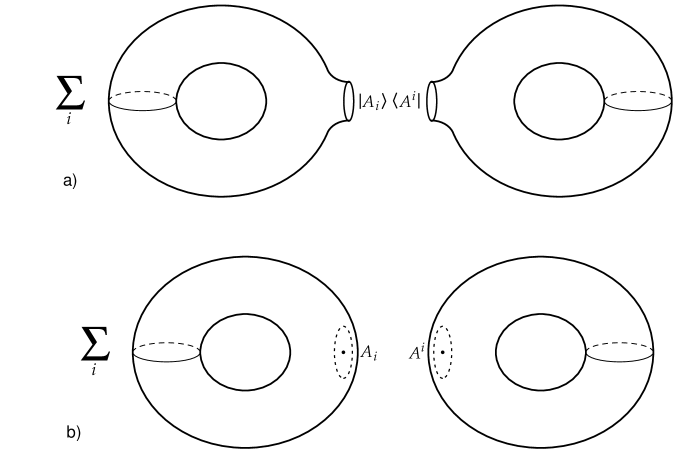
Figure 8: a) Path integral on sewn surface of fig. 7 written in terms of a sum over intermediate states. b) Each state replaced by disk with local operator.

Including the radial evolution for general $q$ we have

$$<\ldots_{1}\ldots_{2}>_{\cal M}\ =\sum_{ij}q^{-h_{i}}\bar{q}^{-\tilde{h}_{i}}<\ldots_{1}{\cal A}_{i}>_{{\cal M}_{1}}\ <\ldots_{2}{\cal A}^{i}>_{{\cal M}_{2}},$$ (1.9.12)

where ${\cal M}$ is sewn from ${\cal M}_{1,2}$, the operators are inserted at the origins of the $z^{(1,2)}$ frames, and indices are raised with the inverse of the metric (1.9.6).

By sewing in this way, an expectation value with any number of operators on a general genus surface can be related to the three-point function on the sphere. For example, fig. 9 shows three of the many ways to construct the genus-two surface with four operators.

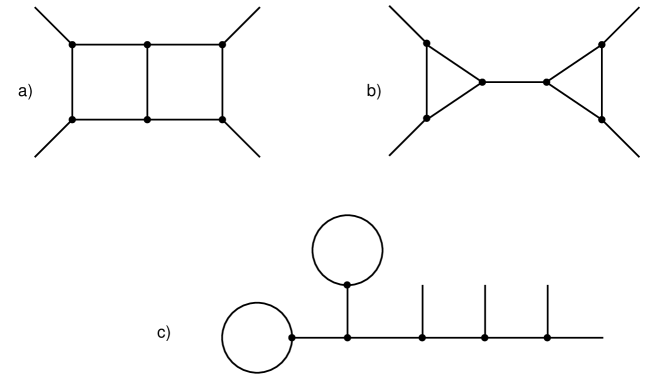
Figure 9: Some sewing constructions of the genus-two surface with four operators. Each vertex is a sphere with three operators, and each internal line represents the sewing construction.

There is one complex modulus $q$ for each handle, or 7 in all here, corresponding to the $3h-3=3$ moduli for the surface plus the positions of the four operators. As a consequence, the OPE coefficients $c_{ij}\!^{k}$ implicitly determine all expectation values, and two CFT’s with the same OPE (and same operator identified as $T(z)$) are the same. However, the $c_{ij}\!^{k}$ are not arbitrary because the various methods of constructing a given surface must agree. For example, the constructions of fig. 9a and 9b differ only by a single move described earlier corresponding to associativity of the OPE, and by further associativity moves one gets fig. 9c. The amplitudes must also be modular invariant. In fig. 9c we see that the amplitude has been factorized into a tree amplitude times one-loop one-point amplitudes, so modular invariance of the latter is sufficient. It can be shown generally that all constructions agree and are modular invariant given two conditions [41]: associativity of the OPE and modular invariance of the torus with one local operator (which constrains sums involving $c_{ij}\!^{j}$).

The classification of all CFT’s can thus be reduced to the algebraic problem of finding all sets $c_{ij}\!^{k}$ satisfying the constraints of conformal invariance plus these two conditions. This program, the conformal bootstrap [19], has been carried out only for cases where conformal invariance (or some extension thereof) is sufficient to reduce the number of independent $c_{ij}\!^{k}$ to a finite number—these are known as rational conformal field theories.

My description of higher-genus surfaces and the CFT’s on them has been rather implicit, using the sewing construction. This is well-suited for my purpose, which is to understand the general properties of amplitudes. For treatments from a more explicit point of view see refs. [43], [44].

Unoriented surfaces, and surfaces with boundary, are also of interest. In particular, CFT’s with boundary have many interesting condensed matter applications. I do not have time for a detailed discussion, but will make a few comments about boundaries. Taking coordinates such that the boundary is Im$(z)=0$ and the interior is Im$(z)>0$, the condition that the energy-momentum be conserved at the boundary is

$$T(z)=\tilde{T}(z),\qquad{\rm Im}(z)=0.$$ (1.9.13)

It is convenient to use the doubling trick, extending $T$ into the lower half-plane by defining

$$T(z)=\tilde{T}(\bar{z}),\qquad{\rm Im}(z)<0.$$ (1.9.14)

The boundary conditions plus conservation of $T$ and $\tilde{T}$ are all implied by the analyticity of the extended $T$. Then $T$ and $\tilde{T}$ together can be expanded in terms of a single Virasoro algebra, the first of equations (1.4.1). The doubling trick is also useful for free fields. For free scalar with Neumann boundary conditions, $\partial_{n}X=0$, the mode expansion is

$$X(z,\bar{z})=X_{L}(z)+X_{L}(\bar{z}),$$ (1.9.15)

with

$$X_{L}(z)=\frac{x}{2}+i\alpha_{0}\ln z-i\sum_{m\neq 0}\frac{\alpha_{m}}{mz^{m}}.$$ (1.9.16)

There is a factor of 2 difference from the earlier (1.4.23); with this, $x$ is the mean value of $X$ at time $|z|=1$. The commutator $[x,\alpha_{0}]$ is found to be $2i$, so $\alpha_{0}=2k$ where $k$ is the conjugate to $x$. The leading surfaces with boundary are the disk and annulus.

2 String Theory

2.1 Why Strings?

The main clue that leads us to string theory is the short-distance problem of quantum gravity. Figure 10 shows some process, say two particles propagating, and corrections due to one-graviton exchange and two-graviton exchange.

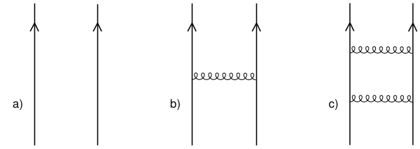
Figure 10: a) Two particles propagating freely. b) Correction from one-graviton exchange. c) Correction from two-graviton exchange.

The one graviton exchange is proportional to Newton’s constant $G_{\rm N}$, which with $\hbar=c=1$ has units of length² or mass^-2: $G_{\rm N}=M_{\rm P}^{-2}$ where the Planck mass $M_{\rm P}=1.2\times 10^{19}$GeV. The dimensionless ratio of the one-graviton correction to the original amplitude must then be of order $E^{2}/M_{\rm P}^{2}$, where $E$ is the characteristic energy of the process. This is thus an irrelevant coupling, growing weaker at long distance, and in particular is negligible at particle physics energies of hundreds of GeV. By the same token, the coupling grows stronger at high energy and at $E>M_{\rm P}$ perturbation theory breaks down. This shows up as the nonrenormalizability of the theory: the two-graviton correction (c) is of order

$$M_{\rm P}^{-4}\int^{\infty}dE^{\prime}E^{\prime 3}$$ (2.1.1)

where $E^{\prime}$ is the energy of the virtual intermediate state, and so diverges if the theory is extrapolated to arbitrarily high energies.

There are two main possibilities. The first is that the theory has a nontrivial ultraviolet fixed point and is fine at high energy, the divergences being an artifact of naive perturbation theory. The second is that there is new physics at some energy and the extrapolation of the low energy theory beyond this point is invalid.

The existence of a nontrivial fixed point is hard to determine. One of the usual tools, Monte Carlo simulation, is extremely difficult because of the need to retain coordinate invariance in the discretized theory. Expansion around the critical dimension $d=2$ indicates a nontrivial UV fixed point when gravity is coupled to certain kinds of matter, but it is impossible to say whether this persists to $d=4$.

The more common expectation, based in part on experience (such as the weak interaction), is that the nonrenormalizability indicates a breakdown of the theory, and that at short distances we will find a new theory in which the interaction is spread out in spacetime in some way that cuts off the divergence. At this point the condensed matter half of the audience is thinking, “OK, so put the thing on a lattice.” But it is not so easy. We know that Lorentz invariance holds to very good approximation in the low energy theory, and that means that if we spread the interaction in space we spread it in time as well, with consequent loss of causality or unitarity. Moreover we know that we have local coordinate invariance in nature—this makes it even harder to spread the interaction out without producing inconsistencies.

In fact, we know of only one way to spread out the gravitational interaction and cut off the divergence without spoiling the consistency of the theory. That way is string theory, in which the graviton and all other elementary particles are one-dimensional objects, strings, rather than points as in quantum field theory. Why this should work and not anything else is not at all obvious a priori, but as we develop the theory we will see that if we try to make a consistent Lorentz-invariant quantum theory of strings we are led inevitably to include gravity [46], [47], and that the short distance divergences of field theory are no longer present.

Perhaps we merely suffer from a lack of imagination, and there are many other consistent theories of gravity with a short-distance cutoff. But experience has shown that the divergence problems of quantum field theory are not easily resolved, so if we have even one solution we should take it very seriously. In the case of the weak interaction, for example, there is only one known way to spread out the nonrenormalizable four-fermi theory consistently. That way is spontaneously broken Yang-Mills theory, which did indeed turn out to be the correct theory of the weak interaction. Indeed, we are very fortunate that consistency turns out to be such a restrictive principle, since the unification of gravity with the other interactions takes place at such high energy, $M_{\rm P}$, that experimental tests will be difficult and indirect.

So what else do we find, if we pursue this idea? We find that string theory fits very nicely into the pre-existing picture of what physics beyond the Standard Model might look like. Besides gravity, string theory necessarily incorporates a number of previous unifying ideas (though sometimes in transmuted form): grand unification, Kaluza-Klein theory (unification via extra dimensions), supersymmetry and extended supersymmetry. Moreover it unifies these ideas in an elegant way, and resolves some of the problems which previously arose—most notably difficulties of obtaining chiral (parity-violating) gauge interactions and the renormalizability problem of Kaluza-Klein theory, which is even more severe than for four-dimensional gravity. Further, some of the simplest string theories [48] give rise to precisely the gauge groups and matter representations which previously arose in grand unification. Finally, the whole subject has a unity and structure far nicer than anything I have seen or expect to see in quantum field theory. So I am strongly of the opinion, and I think that almost all of those who have worked in the subject would agree, that string theory is at least a step toward the unification of gravity, quantum mechanics, and particle physics.

In this lecture and the next I will try to sketch our current understanding of the answer to the question posed in the title. Given limits of time and the nature of the audience, I will focus on broad dynamical issues, especially the mechanics by which string theory cuts off gravity in a consistent way. Most notably, spacetime supersymmetry and the superstring will be underemphasized.

There is one graph, fig. 11, that I want to show you before I launch into the introduction to string theory.

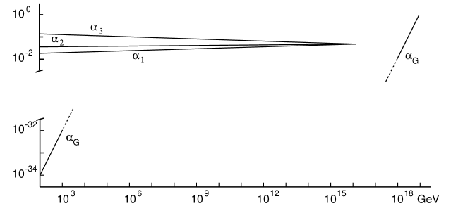
Figure 11: Energy dependence of dimensionless gauge couplings $\alpha_{1,2,3}$ (running logarithmically) and $\alpha_{\rm G}=E^{2}/M_{\rm P}^{2}$.

It shows how the three dimensionless gauge couplings and the dimensionless gravitational coupling $E^{2}/M_{\rm P}^{2}$ depend on energy. The gauge couplings evolve slowly (logarithmically); the big news of recent years is that in the minimal supersymmetric extension of the Standard Model they meet to high accuracy at a common scale, of order $10^{16}$GeV, giving evidence for supersymmetric grand unification [49]. The gravitational coupling starts much smaller but grows as a power and so is just a bit late for its meeting with the others, missing by two orders of magnitude or perhaps a little less. These extrapolations are sensitive to assumptions about the spectrum, so perhaps all four couplings meet at a single energy, a very grand unification. Or perhaps there is a small hierarchy of scales near the Planck scale. But the near meeting in this minimal extrapolation suggests that nature may have been kind and put little new physics between current energies and the Planck scale. With the thorough exploration of the weak interaction scale in coming years, and hopefully the discovery of supersymmetry, we will have several additional extrapolations of the same sort and so several handles on physics near the Planck scale. Also, proton decay reaches into the same region, and if we are lucky it will occur at a rate that will one day be seen.

2.2 String Basics

We want to describe the dynamics of one-dimensional objects. The first thing we need is an action, and the simplest that comes to mind is the Nambu-Goto action,

$$S = -\frac{1}{2\pi\alpha^{\prime}}(\mbox{Area of world-sheet})$$ (2.2.1)

$$= -\frac{1}{2\pi\alpha^{\prime}}\int d^{2}\sigma\,\sqrt{-\det\partial_{a}X^{\mu}\partial_{b}X_{\mu}}\ .$$

This generalizes the relativistic action for a point particle, which is minus the mass times the invariant length of the world-line. For a static string, this action reduces to minus the length of the string times the time interval times $1/2\pi\alpha^{\prime}$, so the latter is the string tension. Note that in the second line we are describing the world-sheet by $X^{\mu}(\sigma_{1},\sigma_{2})$, using a parameterization $\sigma^{a}$ of the world-sheet, but the action is independent of the choice of parameterization (world-sheet coordinate invariant). This will play an important role soon.

In quantum field theory we are familiar with a variety of one-dimensional objects—magnetic flux tubes in superconductors and other spontaneously broken gauge theories, color-electric flux tubes in QCD. Also, the classical statistical mechanics of membranes is given by a sum over two-dimensional surfaces, and so is closely related to the quantum-mechanical path integral for the string. In all of these cases the leading term in the action is the tension (2.2.1). But these are all composite objects, with a thickness, and so there will be higher-dimension terms in the action, such as a rigidity term, multiplied by powers of the thickness. The strings I am talking about, the ‘fundamental’ strings which give rise to gravity, are exactly one-dimensional objects, of zero thickness. Composite strings also have a large contact interaction when they intersect; fundamental strings do not. Fundamental strings are thus simpler than the various composite strings, simpler in particular than the hypothetical string theory of QCD. Nevertheless there has been a great deal of cross-fertilization between the theories of fundamental and composite strings.

It is useful to rewrite the action (2.2.1) in a form which removes the square root from the derivatives. Add a world-sheet metric $g_{ab}(\sigma)$ and let

$$S_{\rm P}=\frac{1}{4\pi\alpha^{\prime}}\int d^{2}\sigma\,\sqrt{g}g^{ab}\partial_{a}X^{\mu}\partial_{b}X_{\mu}\ ,$$ (2.2.2)

where $g=\det g_{ab}$. This is commonly known as the Polyakov action because he emphasized its virtues for quantization [50]. The equation of motion for the metric determines it up to a position-dependent normalization

$$g_{ab}\ \propto\ \partial_{a}X^{\mu}\partial_{b}X_{\mu};$$ (2.2.3)

inserting this back into the Polyakov action gives the Nambu action. Now, the Polyakov action makes sense for either a Lorentzian metric, signature $(-,+)$, or a Euclidean metric, signature $(+,+)$. Much of the development can be carried out in either case. These are presumably related by a contour rotation in the integration over metrics, since the light-cone quantization (Lorentzian) gives the same theory as the Euclidean Polyakov quantization that I will describe. The relation between path integrals over Lorentzian and Euclidean metrics is a complicated and confusing issue in four-dimensional gravity. It seems to work out simply in two dimensions, though I don’t have a simple explanation of why—the demonstration of the equivalence is rather roundabout [52]. Perhaps it is simply that there is enough gauge symmetry to remove the metric entirely. In any case I will take a Euclidean metric henceforth as defining the theory.

In addition to the two-dimensional coordinate invariance mentioned earlier (diff invariance for short),

$$X^{\prime}(\sigma^{\prime})=X(\sigma),\qquad\frac{\partial\sigma^{\prime a}}{\partial\sigma^{c}}\frac{\partial\sigma^{\prime b}}{\partial\sigma^{d}}g^{\prime}_{ab}(\sigma^{\prime})=g_{cd}(\sigma)\ ,$$ (2.2.4)

the Polyakov action has another local symmetry, Weyl invariance, position-dependent rescalings of the metric,

$$g^{\prime}_{ab}(\sigma)=e^{2\omega(\sigma)}g_{ab}(\sigma).$$ (2.2.5)

To proceed with the quantization we need to remove the redundancy from the local symmetries, to fix the gauge. Noting that the metric has three components and there are three local symmetries (two coordinates and the scale of the metric), it is natural to do this by conditions on the metric, setting

$$g_{ab}(\sigma)=\delta_{ab}.$$ (2.2.6)

This is always possible at least locally. The Polyakov action (2.2.2) then reduces to $D$ copies of the earlier scalar action (1.1.1), provided that we choose units such that $\alpha^{\prime}$, which has units of length-squared, is equal to 2.

It is not an accident that the gauge-fixed action is conformally invariant. Fixing the flat metric does not fully determine the local coordinate system. From the discussion of conformal invariance we know that if two coordinate systems are related by

$$\sigma^{\prime 1}+i\sigma^{\prime 2}=f(\sigma^{1}+i\sigma^{2})$$ (2.2.7)

for analytic $f$, the metric changes only by a position-dependent rescaling, so that a Weyl transformation restores it to its original form. In other words, the coordinate transformation (2.2.7) combined with the appropriate Weyl transformation leaves the metric in flat gauge and so is a conformal symmetry of the flat world-sheet action.

So the two-dimensional spacetime of the previous section is now the string world-sheet, while spacetime is the field space where the $X^{\mu}$ live, the target space of the map $X^{\mu}:$ world-sheet $\to$ spacetime.

2.3 The Spectrum

For a closed string, where the spatial coordinate $\sigma^{1}$ is periodic, we can immediately use the earlier results to write down the spectrum. We have $D$ sets of harmonic oscillators,

$$[\alpha^{\mu}_{m},\alpha^{\nu}_{n}]=m\delta_{m+n,0}\eta^{\mu\nu},\qquad[\tilde{\alpha}^{\mu}_{m},\tilde{\alpha}^{\nu}_{n}]=m\delta_{m+n,0}\eta^{\mu\nu},$$ (2.3.1)

the covariant generalization of the earlier commutator, as well as the $D$ momenta $\alpha^{\mu}_{0}=\tilde{\alpha}^{\mu}_{0}=k^{\mu}$. Starting from the states $|0,k\rangle$ which are annihilated by the $m<0$ modes, we build the spectrum by acting any number of times with the $m>0$ modes. By choice of conformal gauge, the string thus separates into a superposition of harmonic oscillators.

But there is one more point to deal with. The index $\mu$ on the oscillators (2.3.1) runs over $D$ values. A string stretched out in the $X^{1}$-direction should by able to oscillation in the $D-2$ transverse directions $\mu=2,\ldots,D-1$, but oscillation along the $X^{1}$-direction leaves the world-sheet unchanged—according to the earlier discussion it is just an oscillation of the parameterization $\sigma$. The same is true of oscillation in the $X^{0}$-direction. It is essential that this be true, because from the oscillator algebra we have the inner product

$$\langle\!\langle 0,k|\alpha^{\mu}_{1}\alpha^{\nu}_{-1}|0,k^{\prime}\rangle=(2\pi)^{D}\delta^{D}(k-k^{\prime})\eta^{\mu\nu}.$$ (2.3.2)

The timelike oscillation $\alpha^{\nu}_{0}|0,k^{\prime}\rangle$ thus has a negative norm and so had better not be in the Hilbert space of the theory.

The point is that when we fix $g_{ab}$ we lose the equations of motion we get from varying $g_{ab}$, and we have to restore them as constraints. Varying the metric gives

$$T_{ab}=0.$$ (2.3.3)

In fact $T_{z\bar{z}}$ vanishes as a consequence of the $X^{\mu}$ equation of motion, but $T_{zz}$ and $T_{\bar{z}\bar{z}}$ do not. The equation of motion does imply that if they vanish at one time they vanish for all times; this is a general feature of such missing equations of motion. Classically, then, we impose these equations on the initial values; quantum mechanically we impose them on the states. In either case the constraint is then preserved by the dynamics.

Later we will discuss a general and powerful way to implement the constraints, the BRST quantization, but it is useful to proceed first by a bit of trial and error (so-called old covariant quantization [53]). Going to the Laurent modes, we could try to impose $L_{n}|\psi\rangle=0$ for all $n$. But this is inconsistent with the Virasoro algebra, since it would imply that $0=[L_{m},L_{-m}]|\psi\rangle=\frac{c}{12}(m^{3}-m)|\psi\rangle$. Instead we require physical states to satisfy

$$(L_{0}-a)|\psi\rangle\ =\ (\tilde{L}_{0}-a)|\psi\rangle = 0$$

$$L_{n}|\psi\rangle\ =\ \tilde{L}_{n}|\psi\rangle = 0,\qquad n>0\ ,$$ (2.3.4)

allowing a possible ordering constant in the $L_{0}$ condition, which will turn out to be necessary. This implies that matrix elements of (2.3.3) between physical states vanish for all $n$,

$$\langle\psi|(L_{n}-a\delta_{n,0})|\psi^{\prime}\rangle=\langle\psi|(\tilde{L}_{n}-a\delta_{n,0})|\psi^{\prime}\rangle=0,$$ (2.3.5)

the $n<0$ generators annihilating the bra since $L_{-n}=L^{\dagger}_{n}$.

There is one more provision. A state of the form

$$L_{-n}|\chi\rangle+\tilde{L}_{-n}|\tilde{\chi}\rangle,\qquad n>0$$ (2.3.6)

for any $|\chi\rangle,|\tilde{\chi}\rangle$ is orthogonal to all physical states and so is called spurious. A physical state which is also spurious is called null. All physical amplitudes involving such a state vanish, so it is physically equivalent to the zero state. Thus we define an equivalence relation between physical states

$$|\psi\rangle\cong|\psi^{\prime}\rangle\ \ {\rm if}\ \ |\psi^{\prime}\rangle-|\psi\rangle=L_{-n}|\chi\rangle+\tilde{L}_{-n}|\tilde{\chi}\rangle.$$ (2.3.7)

The ‘observable’ Hilbert space is the set of equivalence classes, physical states modulo null states.

Let us see how this works for some of the lowest levels. We focus on the open string because it has only one set of modes. At the first level are the states $|0,k\rangle$, with all internal oscillators in their ground states. The physical state conditions (2.3.4) for $n>0$ all involve lowering operators and so hold. There remains

$$0=(L_{0}-a)|0,k\rangle=(2k^{2}-a)|0,k\rangle.$$ (2.3.8)

Thus we obtain a mass shell condition,

$$M^{2}=-k^{2}=-\frac{a}{2}\ \to\ -\frac{a}{2}\frac{2}{\alpha^{\prime}}=-\frac{a}{\alpha^{\prime}}.$$ (2.3.9)

where we have restored $\alpha^{\prime}$ by dimensional analysis.

At the next level the states are

$$|e,k\rangle=e_{\mu}\alpha^{\mu}_{-1}|0,k\rangle.$$ (2.3.10)

for some polarization vector $e_{\mu}$. The nontrivial physical state conditions are

$$0 = (L_{0}-a)|e,k\rangle\ =\ (2k^{2}+\alpha_{-1}\cdot\alpha_{1}-a)|e,k\rangle\ =\ (2k^{2}+1-a)|e,k\rangle$$

$$0 = L_{1}|e,k\rangle\ =\ 2k\cdot\alpha_{1}|e,k\rangle\ =\ 2k\cdot e|0,k\rangle.$$ (2.3.11)

These give a mass shell condition and a transversality condition on $e$,

$$M^{2}=-k^{2}=\frac{1-a}{\alpha^{\prime}},\qquad k\cdot e=0.$$ (2.3.12)

There is a spurious state,

$$L_{-1}|0,k\rangle=2k\cdot\alpha_{-1}|0,k\rangle.$$ (2.3.13)

Thus $|e,k\rangle$ is spurious for $e^{\mu}\ \propto k^{\mu}$. According to the conditions (2.3.12), this is physical, and so null, only if $k\cdot k=0$, which is the case only if $a=1$.

There are now three cases:
i) If $a<1$, the mass-squared is positive. Going to the rest frame, $k^{\mu}=(m,0,0,\ldots,0)$, the physical state condition $k\cdot e=0$ removes the negative norm timelike polarization and leaves the $D-1$ spacelike polarizations. There are no null states, and the spectrum consists of the $D-1$ positive-norm states of a massive vector particle.
ii) If $a=1$, the mass-squared is zero. Going to a frame in which $k^{\mu}=(\omega,\omega,0,0,\ldots,0)$, the physical states are $e^{\mu}\propto k^{\mu}$ plus the $D-2$ transverse polarizations $\mu=2,\ldots,D-1$. The state $e^{\mu}\propto k^{\mu}$ is null, leaving the $D-2$ positive-norm transverse states of a massless vector particle.
iii) If $a>1$, the mass-squared is negative and we can go to a frame $k^{\mu}=(0,k^{1},0,\ldots,0)$. The physical state condition removes a positive-norm spacelike polarization. There is no null state, so we are left with $D-2$ positive-norm spacelike polarizations and one negative-norm timelike polarization.

Case (iii) is obviously unacceptable, but either (i) or (ii) seem satisfactory so far. It is case (ii) that agrees with the BRST quantization, and also with the light-cone quantization, a different gauge in which the number of oscillators is reduced to $D-24$ from the start. In fact, there is no consistent way known to introduce interactions in case (i).

The result at the next level, states

$$f_{\mu}\alpha^{\mu}_{-2}|0,k\rangle+f_{\mu\nu}\alpha^{\mu}_{-1}\alpha^{\nu}_{-1}|0,k\rangle,$$ (2.3.14)

is quite interesting. It depends on the constant $a$ and also on the spacetime dimension $D$. If $a>1$ or $D>26$, there are negative-norm states. If $a\leq 1$ and $D\leq 26$ the OCQ spectrum has positive norm. For the particular case $a=1$ and $D=26$ the observable spectrum is the same as the BRST and light cone spectra; otherwise there are extra states. The derivation is left to the reader.

This pattern persists at all higher levels as well: the observable spectrum has only positive norm states provided $a\leq 1$ and $D\leq 26$, and if $a=1$ and $D=26$ it is the same as the BRST and light cone spectra. This is the no-ghost theorem for the spectrum. This is our first encounter with the critical dimension; later we will understand it more deeply.

For the value $a=1$, the second level is a massless vector particle, a gauge boson. This implies a spacetime gauge symmetry. In amplitudes this symmetry appears as spacetime (not world-sheet) Ward identities, to the effect that the unphysical polarization is not produced, and the amplitudes for equivalent polarizations $e^{\mu}\cong e^{\mu}+ck^{\mu}$ are equal. We will see how this works when we discuss interactions. Since null and unphysical states appear at all levels, this means that ordinary gauge symmetry is only one piece of some much large gauge symmetry in string theory. We will discuss the form of this later.

Notice also that for $a=1$ the lowest state (2.3.9) is a tachyon, $M^{2}=-1/\alpha^{\prime}$. Since the potential for a scalar field is $\frac{1}{2}M^{2}\varphi^{2}$, this means that the ground state is unstable. (One way to think about this is as resulting from the negative Casimir energy of the $X^{\mu}$’s.) We are using the bosonic string only as a toy model, and are indeed expanding around an unstable state. The superstring does not have a tachyon, though unfortunately time will not permit me in these lectures to give a detailed treatment of this.

The closed string spectrum is just the tensor product of two copies of the above, one right-moving and one left-moving. The lowest state $|0,k\rangle$ satisfies

$$M^{2}=-\frac{4a}{\alpha^{\prime}}.$$ (2.3.15)

The next level

$$|e,k\rangle=e_{\mu\nu}\alpha^{\mu}_{-1}\tilde{\alpha}^{\nu}_{-1}|0,k\rangle$$ (2.3.16)

satisfies

$$M^{2}=\frac{4(1-a)}{\alpha^{\prime}},\qquad k^{\mu}e_{\mu\nu}=k^{\nu}e_{\mu\nu}=0.$$ (2.3.17)

The correct values are again $a=1$, $D=26$, so these states are massless, and there are null states leading to the equivalence relation

$$e_{\mu\nu}\sim e_{\mu\nu}+k_{\mu}\zeta_{\nu}+\zeta^{\prime}_{\mu}k_{\nu}$$ (2.3.18)

with $k\cdot\zeta=k\cdot\zeta^{\prime}=0$. Again letting $k^{\mu}=(\omega,\omega,0,0,\ldots,0)$, a complete set of $(D-2)^{2}$ observable states is obtained from transverse $e_{\mu\nu}$, $\mu,\nu\in 2,\ldots,D-1$. This set can be decomposed under the $SO(D-2)$ transverse rotation group, into a traceless symmetric tensor, antisymmetric tensor and invariant. These are respectively the graviton, antisymmetric tensor, and dilaton. Again there are spacetime gauge invariances associated with the graviton and antisymmetric tensor.

2.4 The Weyl Anomaly

The fact that strings can be consistently quantized only in the critical dimension is due to an anomaly, a quantum violation of the local world-sheet symmetries. To see the anomaly, we will work in a more general gauge in which the gauge symmetry is used to fix the metric to some general form $g_{ab}(\sigma)$, not necessarily flat. The result should be independent of what $g_{ab}(\sigma)$ we choose; let us see if it is. I should warn you that the next lecture or so will get steadily more technical, but then things will get better again. I will try to highlight the main results that we will need later on.

We start by examining the path integral over $X^{\mu}$ in the fixed metric $g_{ab}$. The action is diff $\times$ Weyl invariant, but we have to define the path integration. It is easy to preserve the diff invariance. For example, expand $X^{\mu}(\sigma)$ in a complete set of eigenfunctions of the invariant Laplacian $\nabla^{2}$, and put a cutoff on the eigenvalues. Any cutoff will refer to world-sheet lengths, so the Weyl invariance is not automatically preserved and there may be a Weyl anomaly [54, 50]. We must check the Weyl invariance by explicit calculation. This is one virtue of the Polyakov action—any possible anomaly appears in the Weyl symmetry, which is somewhat easier to work with than an anomaly in the diff invariance.

Let us expand around the flat metric in the plane, $g_{ab}(\sigma)=\delta_{ab}+h_{ab}(\sigma)$. The variation of the action with respect to the metric is the energy-momentum tensor, so to second order in $h_{\bar{z}\bar{z}}$ the path integral is

$$<1>\stackrel{{\scriptstyle O(h^{2})}}{{=}}\frac{1}{8\pi^{2}}\int d^{2}z\,d^{2}z^{\prime}\,h_{\bar{z}\bar{z}}(z,\bar{z})h_{\bar{z}\bar{z}}(z^{\prime},\bar{z}^{\prime})<T_{zz}(z)T_{zz}(z^{\prime})>\ +\ {\rm local}.$$ (2.4.1)

The local term comes from the second order variation of the action; we will not need its explicit form. The expectation value is evaluated on the flat world-sheet, and from the OPE we know it to be

$$<T_{zz}(z)T_{zz}(z^{\prime})>\ =\frac{c}{2(z-z^{\prime})^{4}}=-\frac{c}{12}\partial_{z}^{4}\ln|z-z^{\prime}|^{2}=\frac{\pi c}{6}\partial_{z}^{4}(\partial_{z}\partial_{\bar{z}})^{-1}\delta^{2}(z-z^{\prime},\bar{z}-\bar{z}^{\prime}),$$ (2.4.2)

where $c=D$ for the $X$ theory. Thus the second order term (2.4.1) becomes

$$<1> \stackrel{{\scriptstyle O(h^{2})}}{{=}} \frac{c}{48\pi}\int d^{2}z\,d^{2}z^{\prime}\,\partial^{2}h_{\bar{z}\bar{z}}(z,\bar{z})\frac{1}{\partial\bar{\partial}}\partial^{2}h_{\bar{z}\bar{z}}(z^{\prime},\bar{z}^{\prime})$$ (2.4.3)

$$\to \frac{c}{96\pi}\int d^{2}\sigma\,d^{2}\sigma^{\prime}\,\sqrt{g}R(\sigma)\frac{1}{\nabla^{2}}(\sigma,\sigma^{\prime})\sqrt{g}R(\sigma^{\prime})\ .$$

The second line, using the curvature scalar built from $g_{ab}$, is the unique coordinate invariant form to order $h^{2}$ with the given nonlocal $(z-z^{\prime})^{-4}$ term. Now, under a Weyl transformation $g^{\prime}_{ab}=e^{2\omega}g_{ab}$, the curvature changes

$$\sqrt{g^{\prime}}R^{\prime}=\sqrt{g}R-2\nabla^{2}\omega.$$ (2.4.4)

Thus

$$\delta_{\rm Weyl}<1>\ \stackrel{{\scriptstyle O(h^{2})}}{{=}}\frac{c}{24\pi}<1>\int d^{2}\sigma\,\sqrt{g}R\delta\omega.$$ (2.4.5)

Although derived to second order in the background, the result (2.4.5) is in fact the full answer. Given that the Weyl variation must be local (since it comes from the violation of the symmetry by the cutoff) and that the theory is conformally invariant on the flat world-sheet, eq. (2.4.5) is the only possible form. This goes through for any CFT, so we have the result that if we put a CFT on a curved world-sheet the Weyl-dependence is determined entirely by the central charge of the flat world-sheet theory,

$$\delta_{\rm Weyl}\ln<\ldots>\ =\frac{c}{24\pi}\int d^{2}\sigma\,\sqrt{g}R\delta\omega,$$ (2.4.6)

where as usual the transformation properties of the insertions ‘$\ldots$’ are a separate issue. Also, we can integrate the Weyl anomaly to give the full result

$$<1>\ =\exp\biggl{\{}\frac{c}{96\pi}\int\!\int d\sigma\,d\sigma^{\prime}\,R\nabla^{-2}R\biggr{\}}.$$ (2.4.7)

To complete the determination of the Weyl anomaly we need to carry out the gauge fixing carefully, taking into account the Fadeev-Popov determinant. That is, we write the integral over metrics as in integral over the gauge group times a Jacobian, and divide by the gauge volume. Under a small diff $\times$ Weyl transformation, the change in the metric is

$$\delta g_{ab} = -(\nabla_{a}\delta\sigma_{b}+\nabla_{b}\delta\sigma_{a}-g_{ab}\nabla\cdot\delta\sigma)-g_{ab}(2\delta\omega+\nabla\cdot\delta\sigma)$$ (2.4.8)

$$= -(P_{1}\delta\sigma)_{ab}-2g_{ab}\delta\omega^{\prime}.$$

In the first line we have separated the variation into a traceless part and a part proportional to the metric. In the second line we have defined the differential operator $P_{1}$ taking vectors to traceless symmetric tensors, and absorbed the $\nabla\cdot\delta\sigma$ term in a shift of $\omega$. Short circuiting some formal steps that are parallel to the standard treatment of non-Abelian gauge theories, we get

$$\int[dg]\to\det(P_{1})V_{\rm diff\times Weyl}\ .$$ (2.4.9)

The $\delta\omega^{\prime}$ part being purely local gives a trivial Jacobian, equivalent to local counterterms. Thus,

$$\frac{1}{V_{\rm diff\times Weyl}}\int[dX\,dg]\,e^{-S_{\rm P}[g]}=\det(P_{1})\int[dX]\,e^{-S_{\rm P}}.$$ (2.4.10)

In order to expose the general structure of amplitudes it is useful to rewrite the determinant as a path integral over anticommuting Fadeev-Popov ghost fields. From the definition of Grassman integration we have

$$\int db\,dc\,e^{-bMc}=\int db\,dc\,(1-bMc)=M$$ (2.4.11)

for two anticommuting variables $b,c$. This generalizes to

$$\int{\textstyle\prod_{i}}(db_{i}\,dc_{i})\,e^{-b_{i}M_{ij}c_{j}}=\det M\ ,$$ (2.4.12)

as is evident by diagonalizing $M$. This applies to functional determinants as well, so the path integral (2.4.10) becomes

$$\int[dX\,db\,dc]\,e^{-S_{\rm P}-S_{\rm g}}$$ (2.4.13)

where

$$S_{\rm g}=\frac{1}{2\pi}\int d^{2}\sigma\,\sqrt{g}\,b^{ab}(P_{1}c)_{ab}.$$ (2.4.14)

To see the conformal transformation properties, consider a conformally flat metric

$$g_{ab}(\sigma)=e^{\phi(\sigma)}\delta_{ab}.$$ (2.4.15)

The action (2.4.14) becomes

$$S_{\rm g}=\frac{1}{2\pi}\int d^{2}z\,\Bigl{\{}b_{zz}\partial_{\bar{z}}c^{z}+b_{\bar{z}\bar{z}}\partial_{z}c^{\bar{z}}\Bigr{\}}.$$ (2.4.16)

We have used a convenient trick here. The metric (2.4.15) is not flat, so the covariant derivatives are nontrivial. But for the special case of a $z$ derivative acting on a tensor with only $\bar{z}$ indices, or vice versa, the covariant derivatives reduce to the ordinary ones. We have raised and lowered indices so as to take advantage of this. In the form (2.4.16) it is evident that the action is Weyl-invariant with $c^{z},c^{\bar{z}},b_{zz}$, and $b_{\bar{z}\bar{z}}$ neutral under the Weyl transform. The conformal transformation of these fields comes only from the coordinate transformation, so $c^{z}$ is a $(-1,0)$ tensor, $c^{\bar{z}}$ a $(0,-1)$ tensor, $b_{zz}$ a $(2,0)$ tensor, and $b_{\bar{z}\bar{z}}$ a $(0,2)$ tensor.

The ghosts thus are a $\lambda=2$ $bc$ system. Referring back to the earlier result (1.6.13), the ghost system has central charge $-26$. As we have seen, this determines the Weyl transformation properties, so for the combined $X$ and ghost system we have

$$\delta_{\rm Weyl}\ln<\ldots>\ =\frac{D-26}{24\pi}\int d^{2}\sigma\,\sqrt{g}R\delta\omega.$$ (2.4.17)

So the Weyl invariance is anomalous except in the critical dimension $D=26$ [50]!

Is there any possibility for making sense of the theory without Weyl invariance? One possibility is to make some choice for the scale factor of the metric, but there is no natural way to do this. For example, the rather natural choice $\sqrt{g}=1$ is not diff invariant and just moves the anomaly into that symmetry. The other possibility is to integrate over the scale factor—that is, to treat the theory as one that has only coordinate invariance, and use this to fix only two of the three components of the metric [50]. This is a rather large change in the theory, introducing a new degree of freedom. Such ‘non-critical’ string theories are of great interest, and we will return to them later.

For now, let us just point out the following. We can use the coordinate invariance to bring the metric to the form

$$g_{ab}(\sigma)=e^{\varphi(\sigma)}\hat{g}_{ab}(\sigma),$$ (2.4.18)

where $\varphi(\sigma)$ is to be integrated. Now, this theory has a ‘fake’ Weyl invariance, under which $g_{ab}$ is neutral but

$$\hat{g}_{ab}(\sigma)\to e^{2\omega(\sigma)}\hat{g}_{ab}(\sigma),\qquad\varphi(\sigma)\to\varphi(\sigma)-2\omega(\sigma).$$ (2.4.19)

But this is indistinguishable from a theory in which $\hat{g}_{ab}$ is the ‘real’ metric and $\varphi$ is another field. So we can regard this as a Weyl-invariant theory with an extra degree of freedom. Strominger and Verlinde will be interested in two-dimensional coordinate invariance without Weyl invariance, and will make use of this trick to use techniques from CFT. It is interesting to apply this to a theory whose Weyl-variation comes only from the central charge. Inserting the metric (2.4.18) into the action (2.4.3) and using the relation (2.4.4) gives the $\varphi$-dependent

$$\frac{c}{96\pi}\int d^{2}\sigma\sqrt{\hat{g}}\Bigl{\{}\hat{g}^{ab}\partial_{a}\varphi\partial_{b}\varphi+2\hat{R}\varphi\Bigl{\}}\ .\$$ (2.4.20)

The first term is the same as the action for one of the coordinates $X$, so this looks like an extra dimension. The second term is not translationally invariant, so it means that this theory may have some cosmological interpretation, but is not relevant to the translationally invariant surroundings that we find ourselves in.

It may seem odd that a theory without Weyl invariance can be regarded as having it. This is the first example of a general theme which will arise again, both on the world-sheet and in spacetime. This is that gauge invariance is in the end just a redundancy, though a useful one. We can always add redundant fields and sometimes it is useful to do so, as here where it will enable us to apply critical string methods to the noncritical string.

2.5 BRST Quantization

Representing the Fadeev-Popov determinant in terms of ghosts gives us an even larger Hilbert space, and we need to identify the observable states. This leads us to BRST quantization, which is a general method for quantizing systems with gauge symmetries and is indispensable for understanding the general structure of string amplitudes. One way to motivate it is to imagine some arbitrary small change in the gauge-fixing condition. Thus far we have taken a gauge in which $g_{ab}(\sigma)$ was fixed. That is, $g_{ab}(\sigma)-\overline{g}_{ab}(\sigma)=0$ for some fixed function $\overline{g}_{ab}(\sigma)$. In the previous section we in effect checked that the result was invariant under a Weyl transformation of $\overline{g}_{ab}$. But we could imagine a much more general change of gauge

$$g_{ab}(\sigma)-\overline{g}_{ab}(\sigma)-\delta F_{ab}(g,X)=0\ .$$ (2.5.1)

For example, the ‘manifestly unitary’ light-cone gauge places conditions on $X$ as well as $g_{ab}$; to interpolate between the conformal and light-cone gauges one would have to consider deformations of the form (2.5.1).

In order to derive the full invariance condition, it is useful to take a more general and abstract point of view. Consider a path integral with a local symmetry. The path integral fields are denoted $\phi_{i}$, which in the present case would be $X^{\mu}(\sigma)$ and $g_{ab}(\sigma)$. Here we use a very condensed notation where $i$ labels the field, the component, and also the coordinate $\sigma$. The gauge invariance is $\epsilon^{\alpha}\delta_{\alpha}$, where again $\alpha$ labels component and also coordinate. By assumption the gauge parameters $\epsilon^{\alpha}$ are real, since we can alway separate a complex parameter into its real and imaginary parts. The gauge transformations satisfy an algebra

$$[\delta_{\alpha},\delta_{\beta}]=f_{\alpha\beta}\!^{\gamma}\delta_{\gamma}.$$ (2.5.2)

Now fix the gauge by conditions

$$F^{A}(\phi)=0,$$ (2.5.3)

where again $A$ includes the coordinate. Following the usual Fadeev-Popov procedure, the path integral becomes

$$\int\frac{[d\phi_{i}]}{V_{\rm gauge}}\,e^{-S_{1}}\to\int[d\phi_{i}\,dB_{A}\,db_{A}\,dc^{\alpha}]\,e^{-S_{1}-S_{2}-S_{3}},$$ (2.5.4)

where $S_{1}$ is the original gauge invariant action, $S_{2}$ is the gauge-fixing action

$$S_{2}=iB_{A}F^{A}(\phi),$$ (2.5.5)

and $S_{3}$ is the Fadeev-Popov action

$$S_{3}=b_{A}c^{\alpha}\delta_{\alpha}F^{A}(\phi).$$ (2.5.6)

We have introduced the field $B_{A}$ to produce an integral representation of the gauge-fixing $\delta(F^{A})$.

There are two things to notice about this action. The first is that it is invariant under the Becchi-Rouet-Stora-Tyupin (BRST) transformation [58],

$$\delta_{\rm B}\phi_{i} = -i\epsilon c^{\alpha}\delta_{\alpha}\phi_{i},\qquad\delta_{\rm B}B_{A}\ =\ 0,$$

$$\delta_{\rm B}b_{A} = -\epsilon B^{A},\qquad\delta_{\rm B}c^{\alpha}\ =\ -\frac{i}{2}\epsilon c^{\beta}c^{\gamma}f_{\beta\gamma}\!^{\alpha}.$$ (2.5.7)

Note that the transformation mixes commuting and anticommuting objects, so that $\epsilon$ must be taken to be anticommuting. The original action $S_{1}$ is invariant by itself, because the action of $\delta_{\rm B}$ on $\phi_{i}$ is just a gauge transformation with parameter $c^{\alpha}$. The variation of $S_{2}$ cancels the variation of $b_{A}$ in $S_{3}$, while the variations of $\delta_{\alpha}F^{A}$ and $c^{\alpha}$ in $S_{3}$ cancel. The second key property is that

$$\delta_{\rm B}(b_{A}F^{A})=-i\epsilon(S_{2}+S_{3}).$$ (2.5.8)

Now consider a small local change $\delta F$ in the gauge-fixing condition. The change in the gauge-fixing and ghost actions gives

$$\epsilon\delta\langle\psi|\psi^{\prime}\rangle=-i\langle\psi|\delta_{\rm B}(b_{A}\delta F^{A})|\psi^{\prime}\rangle=\langle\psi|\{Q_{\rm B},b_{A}\delta F^{A}\}|\psi^{\prime}\rangle,$$ (2.5.9)

where we have written the BRST variation as an anticommutator with the corresponding conserved charge $Q_{\rm B}$. For physical states the amplitude must be independent of the gauge condition. In order that this hold for arbitrary $\delta F$, it must be that

$$Q_{\rm B}\mbox{$|\psi\rangle$}=Q_{\rm B}\mbox{$|\psi^{\prime}\rangle$}=0,$$ (2.5.10)

with $Q_{\rm B}^{\dagger}=Q_{\rm B}$. This is the essential condition: physical states must be BRST invariant.

There is one more key idea. In order to move around in the space of gauge choices, the BRST charge must remain conserved. Thus it must commute with the change in the Hamiltonian,

$$0 = [Q_{\rm B},\{Q_{\rm B},b_{A}\delta F^{A}\}]$$ (2.5.11)

$$= Q_{\rm B}^{2}b_{A}\delta F^{A}-Q_{\rm B}b_{A}\delta F^{A}Q_{\rm B}+Q_{\rm B}b_{A}\delta F^{A}Q_{\rm B}-b_{A}\delta F^{A}Q_{\rm B}^{2}$$

$$= [Q_{\rm B}^{2},b_{A}\delta F^{A}].$$

In order for this to vanish for general changes of gauge, we need

$$Q_{\rm B}^{2}=0.$$ (2.5.12)

That is, the BRST charge is nilpotent. You can check that acting twice with the BRST transformation (2.5.7) does indeed leave all fields invariant.

The nilpotence of $Q_{\rm B}$ has an important consequence. A state of the form

$$Q_{\rm B}\mbox{$|\chi\rangle$}$$ (2.5.13)

will be annihilated by $Q_{\rm B}$ for any $\chi$ and so is physical. However, it is orthogonal to all physical states including itself:

$$\mbox{$\langle\psi$}|\Bigl{(}Q_{\rm B}\mbox{$|\chi\rangle$}\Bigr{)}=\Bigr{(}\mbox{$\langle\psi$}|Q_{\rm B}\Bigr{)}\mbox{$|\chi\rangle$}=0$$ (2.5.14)

if $Q_{\rm B}\mbox{$|\psi\rangle$}=0$. All physical amplitudes involving such a null state thus vanish. Two physical states which differ by a null state,

$$\mbox{$|\psi^{\prime}\rangle$}=\mbox{$|\psi\rangle$}+Q_{\rm B}\mbox{$|\chi\rangle$}$$ (2.5.15)

will have the same inner products with all physical states and are therefore indistinguishable. So we again identify the observable Hilbert space as a set of equivalence classes, the cohomology of $Q_{\rm B}$. Following terminology from cohomology, a BRST-invariant state is also called closed, and a null state exact.

Applying this to string theory [59] gives the BRST transformation

$$\delta_{\rm B}X^{\mu}=i\epsilon(c\partial+\tilde{c}\bar{\partial})X^{\mu}$$

$$\delta_{\rm B}c=i\epsilon(c\partial+\tilde{c}\bar{\partial})c\qquad\delta_{B}\tilde{c}=i\epsilon(c\partial+\tilde{c}\bar{\partial})\tilde{c}$$

$$\delta_{\rm B}b=i\epsilon(T^{X}+T^{\rm g})\qquad\delta_{\rm B}\tilde{b}=\epsilon(\tilde{T}^{X}+\tilde{T}^{\rm g}),$$ (2.5.16)

where the energy-momentum tensor has been divided into matter and ghost parts. Noether’s theorem gives the BRST current

$$j_{\rm B}=cT^{X}+\frac{1}{2}:\!cT^{\rm g}\!:=cT^{X}+:\!bc\partial c\!:,$$ (2.5.17)

and correspondingly for $\bar{j}_{\rm B}$. (A total derivative can be added to make this a tensor.) This form is rather general: the $c$-ghost times the matter gauge current plus half the ghost gauge current.

Based on our previous experience, we expect that something will go wrong outside the critical dimension. The problem is with $Q_{\rm B}^{2}$. We can calculate this from the $j_{\rm B}j_{\rm B}$ OPE, but the following gives a slight shortcut. The OPE

$$j^{B}(z)b(0)\sim-\frac{1}{z^{2}}:\!bc(0)\!:+\frac{1}{z}(T^{X}(0)+T^{\rm g}(0))$$ (2.5.18)

gives the commutator for the corresponding charge,

$$\{Q_{\rm B},b_{m}\}=L^{X}_{m}+L^{\rm g}_{m}.$$ (2.5.19)

Exercise: Using this anticommutator and the Jacobi identity, show that $\{[Q_{\rm B},L^{X}_{m}+L^{\rm g}_{m}],b_{n}\}$ vanishes if and only if the total central charge $D-26$ vanishes. This implies in fact that $[Q_{\rm B},L^{X}_{m}+L^{\rm g}_{m}]=0$, because by ghost number any term in the commutator would have to contain at least one $c$ mode. Now extend this to $[\{Q_{\rm B},Q_{\rm B}\},b_{n}]$: it vanishes, and so also does $\{Q_{\rm B},Q_{\rm B}\}$, if and only if $D=26$.
So the Weyl anomaly shows up as an anomaly in the nilpotence $Q_{\rm B}^{2}=0$ [59], which is necessary for the consistency of the formalism.

To see how all the formalism works, let us look again at the lowest levels of the open string. There is one more condition that must be imposed on the states, namely

$$b_{0}|\psi\rangle=0.$$ (2.5.20)

The way I think about this is that when we work out the interactions later on we will find that the string propagator always includes a factor $b_{0}$, which projects onto states satisfying (2.5.20) because $b_{0}b_{0}=0$. Recalling the notation (1.6.16), this means that we are interested in states built with raising operators acting on the ghost vacuum $|\!\downarrow\rangle$. The condition (2.5.20) implies in turn that physical states satisfy

$$\{Q_{\rm B},b_{0}\}|\psi\rangle=(L^{X}_{0}+L^{\rm g}_{0})|\psi\rangle=0,$$ (2.5.21)

where $L^{X}_{0}+L^{\rm g}_{0}=2k^{2}+{\sf L}-1$, with ${\sf L}={\sf L}^{X}+{\sf L}^{\rm g}$ the total ghost plus $X$ excitation level, while the total normal ordering constant is taken from the earlier result (1.6.17). The condition (2.5.21) thus relates the mass of a string state to its level of excitation,

$$M^{2}=\frac{{\sf L}-1}{2}$$ (2.5.22)

In terms of the modes,

$$Q_{\rm B}=\sum_{n=-\infty}^{\infty}c_{n}L^{X}_{-n}+\sum_{m,n=-\infty}^{\infty}\frac{(m-n)}{2}(c_{m}c_{n}b_{-m-n})_{{}_{\it CA}}-c_{0}\ ,$$ (2.5.23)

where the subscript CA denotes creation-annihilation normal ordering. The $c_{0}$ term comes from the normal ordering constant in $L_{0}^{\rm g}$, as follows from $\{Q_{\rm B},b_{0}\}=L^{X}_{0}+L^{\rm g}_{0}$.

At the lowest level, ${\sf L}=0$, the states are $|\!\downarrow,0,k\rangle$, denoting the ghost vacuum, $X$ vacuum and momentum. Then

$$0=Q_{\rm B}|\!\downarrow,0,k\rangle=(2k^{2}-1)c^{0}|\!\downarrow,0,k\rangle,$$ (2.5.24)

giving the same mass shell condition as in the old covariant quantization. In this formalism, the constant $a=1$ is from the ghosts. There are there are no exact states at this level, so we have the same tachyon states as before.

At the next level, $N=1$, there are 26+2 states,

$$|\psi\rangle=(e\cdot\alpha_{-1}+\beta b_{-1}+\gamma c_{-1})|\!\downarrow,0,k\rangle,$$ (2.5.25)

depending on a 26-vector $e_{\mu}$ and two constants $\beta$ and $\gamma$. The BRST condition is

$$0=Q_{\rm B}\mbox{$|\psi\rangle$}=2(k^{2}c_{0}+k\cdot ec_{-1}+\beta k\cdot\alpha_{-1})|\!\downarrow,0,k\rangle,$$ (2.5.26)

so an invariant state satisfies $k^{2}=0$ and $k\cdot e=\beta=0$. There are $26$ linearly independent states left. A general $|\chi\rangle$ is of the same form (2.5.25) with constants $e^{\prime}_{\mu}$, $\beta^{\prime}$, $\gamma^{\prime}$, so the general BRST-exact state at this level, with $k^{2}=0$, is

$$Q_{\rm B}\mbox{$|\chi\rangle$}=2(k\cdot e^{\prime}c_{-1}+\beta^{\prime}k\cdot\alpha_{-1})|\!\downarrow,0,k\rangle.$$ (2.5.27)

Thus the ghost state $c_{-1}\mbox{$|0;k\rangle$}$ is BRST-exact, while the polarization is transverse with the equivalence relation $e_{\mu}\cong e_{\mu}+2\beta^{\prime}k_{\mu}$. This leaves the $24$ positive-norm states expected for a massless vector particle.
Exercise: Do the first massive level.

This pattern is general: with the ghosts there are $26+2$ oscillators at each level. The BRST condition eliminates two of these, and two others are exact, leaving $26-2$ oscillators. The BRST quantization is equivalent to the old covariant and light-cone quantizations [59], [60]. In fact, the BRST quantization reduces to the old covariant quantization if we consider only states where the ghosts are in their ground state. The no-ghost theorem states that every cohomology class includes a state of this form. The generalization to the closed string is again straightforward, with $k^{\mu}\to k^{\mu}/2.$

This derivation of the BRST formalism makes it look like a consequence of gauge fixing, but should be thought of as more fundamental. It carries the full information of the original gauge symmetry; in effect, we increase the redundancy of the theory by the addition of the ghosts, but the BRST principle then singles out the physical observables. When we try to generalize string theory, it is generally easiest to generalize it within the BRST formalism, rather than the locally invariant formalism.

It is worth noting that in most familiar circumstances, Ward identities are important but are only part of the story—one also has dynamics. But string theory has coordinate invariance, both on the world-sheet and in spacetime, so that time itself is a gauge degree of freedom. As a consequence the dynamics becomes part of the constraints. As an example, the mass shell condition (which is the Fourier transform of a Klein-Gordon equation in spacetime) arose from the physical state condition.

2.6 Generalizations

We have developed the importance of the Weyl invariance, and its relation to the central charge and the nilpotence of the BRST operator. Now we are in a position to state one answer to the question, “What is the most general consistent string theory?” We will restrict attention to theories for which the action for the embedding time takes the Polyakov form

$$-\frac{1}{8\pi}\int d^{2}\sigma\,\sqrt{g}g^{ab}\partial_{a}X^{0}\partial_{b}X^{0}\ .$$ (2.6.1)

That is, the theory is stationary, and (jumping ahead a bit) the spacetime metric has $G_{0\mu}=-\delta_{0\mu}$. Even in field theory, non-stationary situations are more complicated. There is no longer a distinguished zero-particle vacuum state, and the meaning of a ‘particle’ becomes ambiguous. This subject is much less developed in string theory, and I will avoid it here.

Now, the immediate problem is the one we have discussed, that the quantization of the action (2.6.1) leads to negative norm states, and we need the observable spectrum to have a positive norm. The general solution is simply stated: it depends only on the local symmetry, or BRST invariance, being preserved. That is, the no-ghost theorem holds if we replace the 25 spatial $X^{\mu}$ fields with any $(c,\tilde{c})=(25,25)$ unitary CFT. In particular, the calculation of $Q_{\rm B}^{2}$ goes precisely as before, with $T^{X}$ replaced by the $T$ of the CFT. The unitary condition is necessary because we do not want any other negative norm states besides those from $X^{0}$. Needless to say this generalization has something to do with the idea of compactifying some of the spatial dimensions, but we will discuss this in section 3. We have not yet described string interactions, but this is also the condition under which we can introduce consistent interactions (the CFT must satisfy the two conditions discussed earlier, OPE associativity and one-loop one-point modular invariance).

I should emphasize that all of these theories have tachyons. Whatever the spatial CFT is, it contains the unit operator. The state $|0,k^{0}\rangle$ from the $X^{0}$ theory times $|1\rangle$ from the spatial theory is in the physical spectrum for $1=L_{0}=-\frac{1}{2}(k^{0})^{2}$, which is unstable (tachyonic). To eliminate the tachyon we have to generalize in a different way, enlarging the world-sheet gauge symmetry. Everything that we have done generalizes readily to the $N=1$ superconformal algebra [32], [33]. A simple $N=1$-invariant extension of the bosonic string action uses $D$ copies of the theory (1.7.7),

$$S=\frac{1}{4\pi}\int d^{2}z\,\Bigl{\{}\partial X^{\mu}\bar{\partial}X_{\mu}+\psi^{\mu}\bar{\partial}\psi_{\mu}+\tilde{\psi}^{\mu}\partial\tilde{\psi}_{\mu}\Bigr{\}}\ .$$ (2.6.2)

To be precise this is $(1,1)$ supersymmetric, with one analytic and one antianalytic supercurrent. To build a BRST charge we need a $bc$ or $\beta\gamma$ theory for each gauge current, with the $b$ or $\beta$ ghost having the same weight and opposite statistics from the current. So in this case we need a $\lambda=2$ $bc$ system and a $\lambda=\frac{3}{2}$ $\beta\gamma$ system. The BRST current follows the same pattern as (2.5.17),

$$j_{\rm B}=cT^{X}+\gamma T^{X}_{F}+\frac{1}{2}:\!(cT^{\rm g}+\gamma T^{\rm g}_{F})\!:\ .$$ (2.6.3)

This is nilpotent in the critical dimension, which is again where the total central charge vanishes. The $\beta\gamma$ ghosts contribute $c=\tilde{c}=11$, while each $\psi^{\mu}$ contributes $\frac{1}{2}$, for

$$c=\tilde{c}=\frac{3}{2}D-26+11\ \Rightarrow\ D_{crit}=10.$$ (2.6.4)

Both the $\psi^{0}$ and $\alpha^{0}$ oscillators create negative norm states, which in the critical dimension are removed by the constraints. The spectrum is equivalent to the light-cone gauge, in which only $D-2$ transverse sets of modes remain. The same generalization as above can be made: replace the 9 spatial $X\psi$ theories with any $(c,\tilde{c})=(\frac{27}{2},\frac{27}{2})$ unitary $(1,1)$ super-CFT.

The details of the spectrum—constraints from modular invariance, the GSO projection, absence of tachyons, and spacetime supersymmetry—make a long story that we do not have time for. Let me just mention that in the Ramond sector (integer modes) the Ramond generator $G_{0}$ is

$$G_{0}=k_{\mu}\psi^{\mu}+\ldots,$$ (2.6.5)

terms with lowering operators being omitted, and

$$\{\psi^{\mu}_{0},\psi^{\nu}_{0}\}=\eta^{\mu\nu}.$$ (2.6.6)

The algebra (2.6.6) is the same as that of the Dirac matrices, and its unique representation is the $2^{D/2}$-dimensional Dirac spinor representation. The $G_{0}$ constraint then gives the Dirac equation, just as the $L_{0}$ constraint gave the Klein-Gordon equation.

The analytic and antianalytic constraint algebras need not be the same [61]. The $(1,0)$ heterotic string combines an analytic $N=1$ superconformal symmetry with antianalytic conformal symmetry. The ghosts have central charge $(c,\tilde{c})=(-15,-26)$. For $D=10$ the action (2.6.2) with $\tilde{\psi}$ omitted has central charge $(15,10)$, so an additional $(0,16)$ is needed from another unitary CFT. The constraints of modular invariance are strong, and the only solutions are an $E(8)\times E(8)$ or $SO(32)$ level 1 current algebra [61], [62]. The generalization is to combine the $(c,\tilde{c})=(\frac{3}{2},1)$ CFT from $\mu=0$ with the ghosts plus any $(c,\tilde{c})=(\frac{27}{2},25)$ theory with $(1,0)$ superconformal symmetry. This string is the most promising for a unified theory, the superconformal side eliminating the tachyon and producing spacetime supersymmetry, and the side with the current algebra giving rise to the gauge symmetries.

Moving on, the $N=2$ superconformal algebra needs $\lambda=2$ and $\lambda=1$ $bc$ systems plus two $\lambda=\frac{3}{2}$ $\beta\gamma$ systems for total central charge $-26-2+2\cdot 11=-6$. The basic free representation consists of one complex $X$ and one complex $\psi$ (= two real) for $c=3$, so the critical theory has two such representations. As usual the constraints remove two sets of modes, leaving in this case zero transverse dimensions. The only degree of freedom is a scalar from the center of mass motion of the string. Nevertheless, there is some interesting structure [63].

Higher-$N$ extended superconformal algebras have zero or negative critical dimension. These are the only possibilities as long as we are restricted to half-integer spins $\leq 2$. Both the fractional case [64] and the higher spin case [65] (particularly $W_{3}$) are under investigation. In the fractional case, the OPE has branch cuts so a projection is needed to get well-defined amplitudes. For both cases the product of two representations is not a representation, owing to the nonlocality in the fractional case and the nonlinearity in the $W_{3}$ case. This has made it hard to find theories with a spacetime interpretation, and also makes it hard to construct the BRST operator (since the ghosts and matter do not separate). For $W_{3}$, a theory with a spacetime interpretation has been found and the BRST operator constructed, but the result is disappointing: it turns out to be a special case of the bosonic string. So the theories described above are for now the most general known.

String theories are also distinguished by the world-sheet topologies allowed: closed only, or with boundaries, and oriented only, or unoriented also. Boundaries must be consistent with the constraint algebra, as in eq.(1.9.13) for the conformal case. In particular, the constraint algebra must be left-right symmetric, so that boundaries are not possible in the heterotic case. Unoriented surfaces are allowed only if the full world-sheet action is invariant under world-sheet parity (exchange of $z$ and $\bar{z}$). Theories without boundaries have closed strings only; theories with boundaries have both closed and open strings. There are no string theories with open strings alone—a surface with boundary can be cut open along a curve running from boundary to boundary, corresponding to open string intermediate states, or along a closed curve, corresponding to closed string intermediate states. Inclusion of unoriented surfaces has the effect of projecting the spectrum onto states of even parity.

2.7 Interactions

For composite strings, there are a variety of contact and long-range interactions. In the fundamental string, such interactions cannot be introduced without spoiling the local symmetries, and are not possible. The only interactions that are possible are those that are already contained in the sum over all surfaces. For example, fig. 12 shows a world-sheet in which one closed string splits into two, or the time-reversed process in which two join into one.

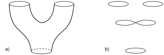
Figure 12: a) World-sheet of closed string splitting. b) Time slices of this process.

Figure 13 shows two strings scattering by exchange of one or two strings.

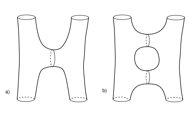
Figure 13: String analogs of fig. 10bc: closed strings scattering by exchange of one string (a) or two strings (b).

Since the string spectrum includes the graviton, these amplitude include the gravitational processes discussed earlier. But now there is no short-distance divergence because the interaction is spread out. I will be describing in somewhat more detail how this works.

Now it is perhaps time to mention an additional term that can appear in the Polyakov action. This is $\Phi_{0}\chi$, with $\Phi_{0}$ a parameter and

$$\chi=\frac{1}{4\pi}\int\sqrt{g}R,$$ (2.7.1)

$R$ again being the world-sheet curvature. This is not merely diff $\times$ Weyl invariant, it is topologically invariant. For a closed surface with $h$ handles $\chi$ is the Euler number $\chi=2-2h$. Adding a handle, as in going from the one-string to the two-string exchange in fig. 13, the path-integral weight $e^{-\Phi_{0}\chi}$ changes by $e^{2\Phi_{0}}$. So while this term does not affect anything local like the world-sheet equations of motion, it does affect the relative weights of surfaces of different topologies. Adding a handle is like adding two trilinear closed string interactions, so the closed string coupling $g_{\rm c}$ depends on $\Phi_{0}$ as $e^{\Phi_{0}}$. For world-sheets with boundaries, as in open string theory, diff $\times$ Weyl invariance requires also a surface term

$$\chi=\frac{1}{4\pi}\int d^{2}\sigma\,\sqrt{g}R+\frac{1}{2\pi}\int_{\rm boundary}ds\,k$$ (2.7.2)

where $k$ is the geodesic curvature of the boundary; in terms of the tangent and normal vectors, $k=t^{a}n_{b}\nabla_{a}t^{b}$. Again this is purely topological, $\Phi_{0}$ times the Euler number. For a compact surface with $h$ handles and $b$ boundaries the Euler number is $2-2h-b$. For the open string amplitudes analogous to fig. 13, with a pair of open strings exchanging one or two open strings, adding a strip increases $b$ by one and so the path integral weight changes by $e^{\Phi_{0}}$. Thus the coupling $g_{\rm o}$ of three open strings goes as $e^{\Phi_{0}/2}$. This will play an important role at a later point, so let me emphasize it: in theories with both open and closed strings, the couplings are related

$$g_{\rm c}\sim g_{\rm o}^{2}.$$ (2.7.3)

For both particle physicists and condensed matter physicists, the natural thing to try do at this point is to calculate a Green’s function, a propagator. Since we are talking about one-dimensional objects, this would be the amplitude to propagate from a given initial configuration to a given final configuration, the sum over all surfaces bounded by these two loops. However, while this seems like a very natural thing to do it is actually extremely hard to carry out consistent with the diff $\times$ Weyl invariance. One already sees this in that the physical state conditions require strings to be on-shell, $k^{2}=-m^{2}$. Any local source in spacetime would couple to all momenta, not just those on the mass shell. This should not be a surprise, because this theory has spacetime gravity, so we have to have observables which are spacetime coordinate-invariant. It is extremely clumsy to try to describe the position and shape of a loop in a coordinate-invariant way.

What can be easily defined in an invariant way is the S-matrix, for scattering from some set of incoming strings to some set of outgoing strings. Effectively the sources have been taken to infinity. Each of the external strings is a semi-infinite cylinder in a world-sheet coordinate $w$. We are familiar with the mapping $z=e^{-iw}$ which takes this to the interior of the disk, with $-i\infty$ mapped to the origin. As shown in fig. 14, this mapping leaves a compact surface. It may seem that I am being careless in identifying a long cylinder in spacetime with a long cylinder in the world-sheet coordinate, but we will see that long-distance propagation in spacetime in fact comes from the latter.

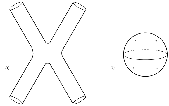
Figure 14: a) $2\to 2$ scattering process. b) Conformally equivalent picture, the cylinders reduced to small holes.

The source which creates the incoming or outgoing string state is then a local operator, known as a vertex operator ${\cal V}$. We are already familiar with the mapping between states and operators. Thus, the tachyon $|0,k\rangle$ with $k^{2}=2$ is created by ${\cal V}=e^{ik\cdot X}$, the graviton, antisymmetric tensor, and dilaton states $\alpha_{-1}^{\mu}\tilde{\alpha}_{-1}^{\nu}|0,k\rangle$ with $k^{2}=0$ are created by ${\cal V}=\partial X^{\mu}\bar{\partial}X^{\nu}e^{ik\cdot X}$, and so on.

In order to make the vertex operator diff-invariant we need to integrate over the world-sheet,

$$V=2e^{\Phi_{0}}\int d^{2}\sigma\,\sqrt{g}{\cal V}\ ,$$ (2.7.4)

where we have included the coupling constant. In flat gauge this becomes

$$e^{\Phi_{0}}\int d^{2}z\,{\cal V}\ .$$ (2.7.5)

Under conformal transformations the measure $d^{2}z$ transforms as a $(-1,-1)$ tensor, so conformal invariance requires that ${\cal V}$ be a $(1,1)$ tensor. This is precisely the OCQ physical state condition (2.3.4), which gives us a simple way to understand the value $a=1$: it makes ${\cal V}$ a (1,1) tensor.

We are led to the following expression for the S-matrix,

$${\sf S}=\sum_{\rm compact\atop topologies}e^{(n-\chi)\Phi_{0}}\int\frac{[dX\,dg]}{V_{\rm diff\times Weyl}}e^{-S_{\rm P}}\,\prod_{i=1}^{n}\int d^{2}\sigma_{i}\,{\cal V}_{i}\ .$$ (2.7.6)

The product runs over the vertex operators incoming and outgoing states, these being distinguished only by the sign of $k^{0}$. (For a general CFT $S_{\rm P}$ is replaced by the appropriate action). We now need to understand how gauge fixing works globally. Locally the number of metric degrees of freedom (three) matches the number of gauge degrees of freedom, but globally there is a small mismatch. In fact, the space of equivalence classes, metrics modulo diff $\times$ Weyl, is identical to a space described earlier in these lectures, the space of Riemann surfaces. Specifying the metric up to Weyl transformations singles out a family of complex coordinates, namely those in which the metric is proportional to $dzd\bar{z}$. This is the definition of a Riemann surface. In the opposite direction, given a Riemann surface we can construct a metric by taking $dzd\bar{z}$ in each patch and smoothing between patches (this can always be done). So this is an isomorphism.

For example, take for the torus the fixed coordinate region $0\leq\sigma^{1}\leq 2\pi$, $0\leq\sigma^{2}\leq 2\pi$ with periodic boundary conditions, so the metric is a doubly periodic function $g_{ab}(\sigma_{1},\sigma_{2})$. Then by coordinate transformations which preserve the periodicity and Weyl transformations we can bring the metric to the form

$$ds^{2}=|d\sigma^{1}+\tau d\sigma^{2}|^{2}\ .$$ (2.7.7)

for some $\tau$. These are the same metrics described earlier in terms of a fixed metric and $\tau$-dependent coordinate region. So after gauge-fixing we are left with an integral over the moduli space of Riemann surfaces, of complex dimension $0$ for $h=0$, 1 for $h=1$ and $3h-3$ for $h\geq 2$. For $h=0,1$ there is the further complication of conformal Killing vectors, gauge symmetries which remain after fixing the metric. These can be fixed by fixing the positions of some vertex operators, 3 at $h=0$ or $1$ at $h=1$. In all, if we have $n$ vertex operators on a genus $h$ surface, the total number of complex moduli (for the metric and the positions) is $3h+n-3$.

To carry out the Fadeev-Popov procedure we trade the original integral $[dg]\,\prod_{i}d^{2}\sigma_{i}$ for $[d\delta\sigma\,d\delta\omega]\,d\vec{t}\,\prod^{\prime}_{i}d^{2}\sigma_{i}$ where $\vec{t}$ are the moduli for the surface and the prime on the product denotes the omission of any fixed vertex operators. The Fadeev-Popov procedure can be carried out as before, giving a mixture of functional and finite-dimensional determinants, which again can be expressed in terms of a path integral over ghosts. I will quote here only the result. The S-matrix for $n$ external strings is given by a sum and path integral

$${\sf S}=\sum_{\rm compact\atop topologies}e^{(n-\chi)\Phi_{0}}\int[dX\,db\,dc]\,e^{-S_{\rm P}-S_{\rm g}}\ \ldots\ .$$ (2.7.8)

The insertions are of three types [20], [67], [9], [18]:
For each modulus (now divided into real parts $t^{r}$), the $b$-ghost insertion

$$\frac{1}{4\pi}\int d^{2}\sigma\,\sqrt{g}b^{ab}\frac{\partial g_{ab}}{\partial t^{r}}\ .$$ (2.7.9)

For each vertex operator which is fixed, the insertion

$$c\tilde{c}{\cal V}_{i}\ .$$ (2.7.10)

For each vertex operator which is integrated, the insertion

$$\int d^{2}\sigma\,\sqrt{g}{\cal V}_{i}\ .$$ (2.7.11)

This can also be expressed in terms of the data which define the Riemann surface, the transition functions. It is convenient to fix every vertex operator, put all the moduli in the transition functions. The vertex operators are then $c\tilde{c}{\cal V}_{i}$ as above, while the $b$-ghost insertions are

$$\frac{1}{2\pi i}\sum_{(mn)}\int_{C_{mn}}\biggl{\{}dz_{m}\frac{\partial f_{nm}}{\partial t^{r}}\biggr{|}_{z_{n}}b_{z_{m}z_{m}}-{d\bar{z}_{m}}\frac{\partial\bar{f}_{nm}}{\partial t^{r}}\biggr{|}_{z_{n}}b_{\bar{z}_{m}\bar{z}_{m}}\biggr{\}}\ ,$$ (2.7.12)

where the sum runs over all pairs of overlapping patches and the integral runs along any curve separating the patches.

Notice that for OCQ-type vertex operators the ghosts are in their vacuum state $|\!\downarrow\downarrow\rangle$, which translates into $c\tilde{c}$. So it is the fixed vertex operators which are given by the state-operator mapping. The integrated vertex operators can be understood as arising from the $b$-ghost insertions for the position. The insertion for translating a little patch containing the vertex operator is $\tilde{b}_{-1}b_{-1}$, giving

$$\tilde{b}_{-1}b_{-1}\cdot c\tilde{c}{\cal V}_{i}={\cal V}_{i}\ ,$$ (2.7.13)

which is the integrated form. The rules in terms of Riemann surfaces, by the way, apply to all BRST-invariant vertex operators, not just the OCQ-type.

2.8 Trees and Loops

To conclude this subject I work out one example and discuss some general principles. For four closed string tachyons on the sphere, fully fixing the gauge invariance leaves one position integrated and three fixed,

$${\sf S}(k_{1},k_{2},k_{3},k_{4})\ =\ e^{2\Phi_{0}}C_{S_{2}}\int d^{2}z_{4}$$ (2.8.1)

$$\qquad\qquad<\tilde{c}ce^{ik_{1}\cdot X}(z_{1},\bar{z}_{1})\,\tilde{c}ce^{ik_{2}\cdot X}(z_{2},\bar{z}_{2})\,\tilde{c}ce^{ik_{3}\cdot X}(z_{3},\bar{z}_{3})e^{ik_{4}\cdot X}(z_{4},\bar{z}_{4})>_{S_{2}},$$

where the integral runs over the complex plane, and $C_{S_{2}}$ is a numerical normalization factor for the path integral on the sphere. The expectation value can be obtained from our earlier results, giving

$${\sf S}(k_{1},k_{2},k_{3},k_{4}) = ie^{2\Phi_{0}}C_{S_{2}}(2\pi)^{26}\delta^{26}({\textstyle\sum_{i}k_{i}})\int d^{2}z_{4}\,|z_{12}|^{2}|z_{13}|^{2}|z_{23}|^{2}\prod_{i<j}|z_{ij}|^{2k_{i}\cdot k_{j}}$$ (2.8.2)

$$\to ie^{2\Phi_{0}}C_{S_{2}}(2\pi)^{26}\delta^{26}({\textstyle\sum_{i}k_{i}})\int d^{2}z_{4}\,|z_{4}|^{2k_{1}\cdot k_{4}}|1-z_{4}|^{2k_{2}\cdot k_{4}}.$$

In the second line we have used the fact that the result is independent of the fixed positions (as can be shown by a Möbius transformation) to move $z_{1}\to 0$, $z_{2}\to 1$, $z_{3}\to\infty$. The integral can be related to gamma functions with the result

$${\sf S}(k_{1},k_{2},k_{3},k_{4}) = ie^{2\Phi_{0}}C_{S_{2}}(2\pi)^{26}\delta^{26}({\textstyle\sum_{i}k_{i}})$$

$$\qquad\qquad\frac{\Gamma(-s/2-1)\Gamma(-t/2-1)\Gamma(-u/2-1)}{\Gamma(-s/2-t/2-2)\Gamma(-t/2-u/2-2)\Gamma(-u/2-s/2-2)},$$

where $s=-(k_{1}+k_{2})^{2}$, $t=-(k_{1}+k_{3})^{2}$, and $u=-(k_{1}+k_{4})^{2}$, and $u+t+s=-8$.

This is the Virasoro-Shapiro amplitude. It has a single pole when $s$, $t$, or $u$ takes a value $-2,0,2,4,\ldots\$. These are the masses of string states and correspond to processes where two of the external strings join into one; the coefficient of the pole is related to the square of the three-point amplitude, which determines $C_{S_{2}}=8\pi^{2}$. The massless pole, for example, has the correct form expected from graviton plus dilaton exchange (the antisymmetric tensor doesn’t contribute due to world-sheet parity symmetry).

The notable feature of this amplitude is its soft high-energy behavior. Using Stirling’s approximation for the exponentials, one finds that at large $s$ and fixed $\theta$ (and so fixed $t/s$, $u/s$) it behaves as

$$e^{-sf(\theta)}$$ (2.8.4)

This is in contrast to similar amplitudes in pointlike field theory, which fall as powers of $s$, and arises from spread-out nature of the string (more on this later).

Now we turn to the one loop amplitude. The one-loop four-point amplitude shown in fig. 15 contains the two-graviton exchange described earlier, which had the severe divergence in field theory.

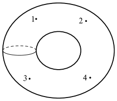
Figure 15: One loop four-string amplitude.

Let us look at the integration over the momentum running around the loop. From the earlier discussion (1.9.9), the path integral translates into a Hamiltonian expression involving

$$e^{2\pi i(\tau L_{0}-\bar{\tau}\tilde{L}_{0})}\ .$$ (2.8.5)

For large loop momenta the dominant term here is

$$e^{-2\pi k^{2}{\rm Im}(\tau)}\ .$$ (2.8.6)

After Wick rotation of $k^{0}$, this is a convergent gaussian at fixed $\tau_{2}$. One might also worry about a divergence from the sum over the string states running around the loop, but in spite of the large number of states the sum is handily convergent at fixed $\tau$ owing to the exponential suppression factor (2.8.5). The region Im$(\tau)\to 0$ is the potential danger, both for the integral over momentum and for the sum over states. But here we run into the happy circumstance that this is not in the range of integration, the moduli space of the torus, shown in fig. 6. There is a lower bound on Im$(\tau)$, so the integral over momenta is gaussian, as would be expected from the high energy behavior (2.8.4). In contrast, in field theory one could write the loop integral in a Schwinger parameterization,

$$\int_{0}^{\infty}ds\,e^{-(k^{2}+m^{2})s}\ ,$$ (2.8.7)

with $s$ being analogous to Im$(\tau)$, but here the integral does indeed run down to $s=0$, leading in the end to a divergent momentum integral. (Cutting off the $s$ integral doesn’t work, as I will explain shortly).

So in this example we see that the would-be ultraviolet region of moduli space is missing. This is a general principle in string theory: all the limits of moduli space can be interpreted as infrared limits. This can already be seen in the Virasoro-Shapiro amplitude. The moduli space has three limits, $z_{4}\to z_{1}$, $z_{4}\to z_{2}$, or $z_{4}\to z_{3}$. The first is shown fig. 16a; it is conformally equivalent to the long cylinder in the fig. 16b, and to the plumbing-fixture construction in fig. 16c with $q\sim z_{4}-z_{1}\to 0$.

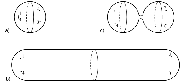
Figure 16: Three pictures of the same limit of moduli space. a) $z_{4}\to z_{1}$ on the sphere. b) Annular region around $z_{1,4}$ conformally transformed to a long cylinder. c) Long cylinder conformally transformed to a pinched cylinder.

In the last form we can use the sewing formula (1.9.12) to express the asymptotics in terms of a sum over intermediate string states. The contribution of state $i$ is proportional to

$$\int_{0}d^{2}q\,|q|^{k^{2}+m_{i}^{2}-2}.$$ (2.8.8)

The integral runs over some neighborhood of the origin. The behavior as $q\to 0$ is dominated by the lightest states. The integral converges when $k^{2}+m_{i}^{2}$ is positive for all states and can be defined elsewhere by analytic continuation. The result has a pole proportional to

$$\frac{1}{k^{2}+m_{i}^{2}}.$$ (2.8.9)

This is the origin of the series of poles in the Virasoro-Shapiro amplitude. These poles correspond to long-distance propagation in spacetime, so as in the discussion of fig. 14 this comes from a degenerating (long) cylinder.

We could extract the asymptotics in this limit $z_{4}\to z_{1}$ directly from the OPE; the sewing formula in this case reduces to the OPE. But the sewing formula is more general. The surface formed by sewing general surfaces ${\cal M}_{1}$ and ${\cal M}_{2}$ is conformally equivalent to a small copy of ${\cal M}_{1}$ inserted into ${\cal M}_{2}$ (and vice versa). The sewing formula related this to a sum of local operators inserted in ${\cal M}_{2}$, generalizing the OPE.

All limits of moduli space are of the same type as this one, with one or more handles degenerating. They can thus be analyzed by means of sewing in the same way. The asymptotics are dominated by the lightest states, and the divergences all arise from intermediate states being on the mass-shell. This corresponds to long-distance propagation in spacetime, and so is an infrared effect. There are no short-distance divergences. As an example, consider the limit of the one-loop four-point amplitude in which all the vertex operators come together, fig. 17a. This looks as though it could produce a short-distance divergence. But, in analogy to the previous fig. 16, this is conformal to fig. 17b in which the vertex operators are at the end of a long cylinder, and to fig. 17c where a sphere and torus are sewn together.

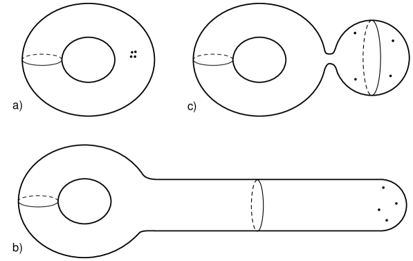
Figure 17: Three pictures of the another limit of moduli space. a) Four vertex operators coming together on the torus. b) Annular region around operators conformally transformed to a long cylinder. c) Long cylinder conformally transformed to a pinched cylinder.

There may indeed be a divergence, but it is an infrared effect, dominated by the lightest states. The momentum flowing through the pinch must be zero by momentum conservation, so the pole (2.8.9) is 1/0 for any massless state. The interpretation is that the one-loop one-point function produces a source for the massless field, so it is necessary to expand around a solution to the loop-corrected equations. This cancels the divergence, and is known as the Fischler-Susskind mechanism [69], [40]. More generally the principle is that all divergences are from long distances and so, as in field theory, go away if one asks the right questions.

Finally a few comments about the general structure of amplitudes. The interactions must respect the BRST invariance. In particular, the amplitude for an exact state $Q_{\rm B}\cdot{\cal V}_{\chi}$ must be zero—this is equivalent the the gravitational Ward identity, together with the corresponding Ward identities for all the higher levels. To see the decoupling of the null state, write $Q_{\rm B}$ as a contour integral around ${\cal V}_{\chi}$. Expand the contour $C$ and contract it down around the other insertions in the path integral. The other vertex operators are BRST invariant and give zero. However, there is a nonzero residue at the $b$ insertions, which by the OPE (2.5.18) is $T^{\rm total}$. In either form (2.7.9) or (2.7.12), this gives a total derivative of the path integral with respect to the moduli. Upon integration over moduli space this becomes a surface term[20], [67], [9], [70]. The surface term vanishes under the same condition that the (analytically continued) integral is finite—that is, unless we are sitting on a pole (in which case the Fischler-Susskind mechanism restores conformal invariance).

Notice that if we mutilate the theory by cutting out parts of moduli space, the total derivative no longer integrates to zero and the theory is inconsistent. The same thing happens in field theory if we try to cut off the Schwinger parameter integral (2.8.7). String theory manages to cut off the modular integral while leaving a smooth moduli space without spurious internal boundaries.

One can also arrive at the rules for the string S-matrix from considerations of BRST invariance, rather than via gauge-fixing. First, as found in the exercise below eq. (1.9.4), ghost number conservation requires the path integral to contain insertions with net $N_{b}-N_{c}=3h-3$; our rules for the string S-matrix are consistent with this. These insertions are BRST invariant only up to a total derivative with respect to the moduli, so the path integral must be integrated over moduli space as found from gauge fixing. In trying to generalize string theory it is often easiest to use this strategy directly to determine the form of the amplitudes, rather than gauge-fixing from a locally-invariant form. For example, superstring amplitudes can in this way be written as an integral over supermoduli space.

This concludes our survey of the current perturbative answer to the question, “what is string theory?” In particular we have seen what are the ingredients that make the perturbation theory consistent.

3 Vacua and Dualities

3.1 CFT’s and Vacua

In the last section we described the most general string theory as defined by the world-sheet gauge algebra, by the world-sheet topologies allowed, and by the particular world-sheet CFT or super-CFT. In this section we will try to get a better understanding of the nature of the space of theories. The main theme is that what we have called different string theories are in many (and possibly all) cases the same theory expanded around a different vacuum state. Moreover, in some cases what appear to be different theories are in fact the same theory in the same vacuum. Some of these connections are well-developed, while others are highly conjectural.

Let us start by trying to understand better the idea of replacing the spatial $X^{\mu}$’s with a more general CFT. I will focus on the bosonic string, but the ideas all generalize to the superstring. For example, replace the Polyakov action with the non-linear sigma model [23]-[25]

$$S_{\Sigma}=\frac{1}{8\pi}\int d^{2}\sigma\,\biggl{\{}\Bigl{(}\sqrt{g}g^{ab}G_{\mu\nu}(X)+i\epsilon^{ab}B_{\mu\nu}(X)\Bigr{)}\partial_{a}X^{\mu}\partial_{b}X^{\nu}+2\sqrt{g}R\Phi(X)\biggr{\}},$$ (3.1.1)

which is the most general coordinate invariant action we can make with two derivatives. This is the same theory (1.6.27) that we have already discussed on a flat world-sheet, and when the $X$-dependence is slow the theory can be studied perturbatively (this is now perturbatively in the world-sheet couplings). This gives rise to a consistent string theory, to leading order in the world-sheet perturbation theory, if

$$2{\bf{R}}_{\mu\nu}+4\nabla_{\mu}\nabla_{\nu}\Phi-\frac{1}{2}H_{\mu\lambda\omega}H_{\nu}{}^{\lambda\omega} = 0$$

$$-\nabla^{\omega}H_{\omega\mu\nu}+2\nabla^{\omega}\Phi H_{\omega\mu\nu} = 0$$

$$D-26-6\nabla^{2}\Phi+12\nabla_{\omega}\Phi\nabla^{\omega}\Phi-\frac{1}{2}H_{\mu\nu\lambda}H^{\mu\nu\lambda} = 0.$$ (3.1.2)

This conformal field theory has an obvious interpretation. The functions $G_{\mu\nu}(X)$, $B_{\mu\nu}(X)$ and $\Phi(X)$ correspond to nontrivial backgrounds of the string graviton, antisymmetric tensor and dilaton. One might have expected something stringier-looking, since the graviton, etc., are supposed to be strings. But we found in our discussion of scattering amplitudes that strings could be created by local vertex operators; the sigma model action can then be thought of from exponentiating the vertex operators, corresponding to a coherent state of strings. Notice in particular that different values of the string coupling $e^{\Phi_{0}}$ are now seen as corresponding to expanding around different backgrounds in a single theory, namely different constant values of the dilaton field $\Phi$. The field equations (3.1.2) arise from a spacetime action

$${\bf{S}}=\frac{1}{2}\int d^{D}X\,\sqrt{-G}e^{-2\Phi}\biggl{\{}-\frac{(D-26)}{3}+{\bf{R}}-\frac{1}{12}H_{\mu\nu\lambda}H^{\mu\nu\lambda}+4\nabla_{\mu}\Phi\nabla^{\mu}\Phi\biggr{\}}.$$ (3.1.3)

Higher orders in the world-sheet perturbation expansion produce terms with more derivatives in the field equations and action.

Each static solution corresponds to a possible ground state. For example, a background with four flat dimensions and the remainder curved on a sufficiently small distance scale $l_{c}$ would look like what we see around us. Even before string theory this was a promising idea for unification. It unites fields of different spins into a single higher-dimensional field (Kaluza-Klein theory), and provides a natural origin for the fermion generations as states with the same gauge quantum numbers but different wavefunctions in the compact dimensions. By the way, we see from the loop correction to the central charge in the last line of eq. (3.1.2) that the number of compact dimensions need not be 22. Actually the expansion which gives rise to eqs. (3.1.2) breaks down when the corrections are of order 1, but exact CFT’s with $D\neq c$ are known. An example is the WZW model, correpsonding to strings propagating on a group manifold [73], [28].

For more general CFT’s, the interpretation in terms of compactification is not so clearcut. But given the many equivalences between two-dimensional field theories (the most familiar being bosonization), it is quite possible that all can be understood in terms of background fields, perhaps including massive string fields. As one example, the minimal models were first constructed in an abstract way, but now several Lagrangian formulations are known. One in particular, the Landau-Ginsburg theory, can be regarded as the string moving in a tachyon background [74]. So the general assumption is that different CFT’s should be regarded as different vacua.

Let us make a few general observations. Just as we have noted that the bosonic string always has a tachyon, it also has a graviton, antisymmetric tensor, and dilaton. The vertex operator $e_{\mu\nu}\partial X^{\mu}\bar{\partial}X^{\nu}e^{ik\cdot X}$, with $e_{\mu\nu}$ and $k_{\mu}$ lying in the noncompact flat directions, is always a $(1,1)$ vertex operator for $k^{2}=0$. The $(1,1)$ and $(1,0)$ superstrings also always include the graviton and tachyon.

If the compact theory has a current algebra, the vertex operator $\partial X^{\mu}\tilde{j}^{a}e^{ik\cdot X}$ or $j^{a}\bar{\partial}X^{\mu}e^{ik\cdot X}$ is $(1,1)$ for $k^{2}=0$ and corresponds to a gauge boson. So the spacetime gauge symmetries are in one-to-one correspondence with the global symmetries (current algebras) of the compact CFT. A similar result, a bit less straightforward to derive, is that there is spacetime supersymmetry if and only if the $N=1$ superconformal constraint algebra of the superstring is embedded in a larger $N=2$ symmetry of the CFT, with a quantization condition on the $U(1)$ charge of the $N=2$ algebra [75].

The number of CFT’s or super-CFT’s of appropriate central charge is enormous, even restricting to those with exactly four noncompact flat directions. We are now interpreting these as different backgrounds within a single theory, but the effective four-dimensional physics is different in each. The problem of finding the right theory is thus transmuted in string theory into the dynamical problem of finding the right background. For backgrounds with spacetime supersymmetry, it is a theorem that they remain stable to all orders of perturbation theory, but it is also known, from the understanding of supersymmetry breaking in field theory, that most are destabilized by non-perturbative effects. Spacetime supersymmetry of the effective field theory below the string scale gives a great deal of information about the dynamics, a subject currently in active development. But it seems likely that dynamics at the string scale will also play an important role. It may also be that there are in the end many stable ground states of string theory, so that the choice between them will be determined in part by the initial conditions.

3.2 Compactification on a Circle

A flat spacetime with one dimension periodic,

$$X^{1}\cong X^{1}+2\pi R$$ (3.2.1)

is the simplest compactification of the bosonic string, but is quite instructive. (Equivalently, let the periodicity be $2\pi$ but $G_{11}=R^{2}$). The periodicity has two effects. The first is that the string wavefunctions must respect it, so

$$k^{1}=\frac{n}{R}$$ (3.2.2)

is quantized. This is the same as for a field theory on this space. The second effect is unique to string theory: a string can be wound around the periodic dimension, so that

$$X^{1}(2\pi)=X^{1}(0)+2\pi mR.$$ (3.2.3)

Referring back to our mode expansion (1.4.23) for the free scalar, we see that this means that the eigenvalues $k^{1}_{L,R}$ of $\alpha_{0}$ and $\tilde{\alpha}_{0}$ are no longer equal, $k^{1}_{L}-k^{1}_{R}=mR$. The total momentum (3.2.2) is $\frac{1}{2}(k^{1}_{L}+k^{1}_{R})$, so

$$k^{1}_{L}=\frac{mR}{2}+\frac{n}{R},\qquad k^{1}_{R}=-\frac{mR}{2}+\frac{n}{R}.$$ (3.2.4)

Also from the expansion (1.4.23), the vertex operator for such a state will be proportional to

$$e^{ik_{L}X_{L}(z)+ik_{R}X_{R}(\bar{z})}.$$ (3.2.5)

Although the $X_{R}X_{R}$ and $X_{L}X_{L}$ OPE’s contain branch cuts, the OPE of any two vertex operators (3.2.5) in the spectrum (3.2.4) is single-valued.

The $L_{0}\pm\tilde{L}_{0}$ physical state conditions thus become

$$M^{2}\ =\ k_{0}^{2}-\sum_{\mu=2}^{25}k_{\mu}^{2}\ =\ \frac{m^{2}R^{2}}{4}+\frac{n^{2}}{R^{2}}+{\sf L}+{\sf\tilde{L}}-2$$

$$mn+{\sf L}-{\sf\tilde{L}}\ =\ 0\ .$$ (3.2.6)

Looking at the massless spectrum, the states

$$\alpha_{-1}^{\mu}\alpha_{-1}^{\nu}|0,m=n=0\rangle,$$ (3.2.7)

with no compact momentum or winding, remain massless. For $\mu$ and $\nu$ both in the range $0,2\ldots,25$, these are just the graviton, dilaton, and antisymmetric tensor of the 25-dimensional theory. When either $\mu=1$ or $\nu=1$ the state is a vector in the noncompact dimensions, a gauge boson. The corresponding vertex operators are

$$(\partial X^{\mu}\bar{\partial}X^{1}\pm\partial X^{1}\bar{\partial}X^{\mu})e^{ik\cdot X}.$$ (3.2.8)

The plus sign comes from the 26-dimensional metric, the Kaluza-Klein mechanism. The minus sign comes from the 26-dimensional antisymmetric tensor, a generalization of the Kaluza-Klein mechanism; call this an $H$ gauge boson. The operator product of the gauge boson vertex operator (3.2.8) with a general vertex operator of momentum $l$ is proportional to $l^{\mu}(l_{L}^{1}\pm l^{1}_{R})$. The Kaluza-Klein and $H$ gauge bosons thus couple to the compact momentum and winding number respectively. Finally, the state (3.2.7) with $\mu=\nu=1$ is a 25-dimensional scalar, and is the metric component corresponding to the radius $R$ of the compact dimension.

So far this is the same as would be found just from the low energy field theory (3.1.3), but this simple theory has some interesting stringy physics. Consider the four sets of states with $|m|=|n|=1$ and ${\sf L}+{\sf\tilde{L}}=1$,

$$\tilde{\alpha}_{-1}^{\mu}|0,m=n=\pm 1\rangle,\qquad\alpha_{-1}^{\mu}|0,m=-n=\pm 1\rangle.$$ (3.2.9)

Their masses are

$$M=|R^{2}-2|/2R.$$ (3.2.10)

Precisely at the radius $R=\sqrt{2}$ these states are massless, and so are gauge bosons. At this radius, the spectrum (3.2.4) includes the four currents

$$:\!e^{\pm iX^{1}_{L}(z)\sqrt{2}}\!:,\quad:\!e^{\pm iX^{1}_{R}(\bar{z})\sqrt{2}}\!:\ .$$ (3.2.11)

Together with the two $U(1)$ currents

$$\partial X^{1}(z),\qquad\bar{\partial}X^{1}(\bar{z}),$$ (3.2.12)

these form an analytic and an antianalytic $SU(2)$ current algebra. This $SU(2)\times SU(2)$ symmetry has nothing to do with the Lorentz invariance of the flat-spacetime theory. Its emergence at the critical radius is an example of the large symmetry that is hidden in string theory, almost completely broken. By the way, the mass of the gauge boson, as $R$ moves away from the critical value, comes from the ordinary Anderson-Higgs mechanism. The vertex operator for a small change in $R$,

$$\partial X^{1}\bar{\partial}X^{1},$$ (3.2.13)

is built out of the $SU(2)$ currents (3.2.12), and so transforms as the $z$-component of a vector under each $SU(2)$, breaking $SU(2)\times SU(2)$ down to the Kaluza-Klein and $H$ $U(1)\times U(1)$.

There is another stringy phenomenon here. As $R\to\infty$, the states with $m\neq 0$ go to infinite mass, while the states with $m=0$, $n\neq 0$ form a continuum. This is simply because it costs an energy of order $R$ to wind around the large dimension, while the momentum in that direction becomes continuous in the limit. This is all as in field theory. But look at $R\to 0$. States with $n\neq 0$ become very massive because of the large compact momentum, just as in field theory. But the states with $n=0$, $m\neq 0$ are now forming a continuum, something which has no analog in field theory. In fact, the spectrum is invariant under R-duality, also known as T-duality,

$$R\leftrightarrow\frac{2}{R},\qquad m\leftrightarrow n,$$ (3.2.14)

which interchanges large and small radius, and interchanges compact momentum with winding number [77]; for recent reviews see [3], [78].

This is not only a symmetry of the spectrum, but also of the interactions. $R$-duality takes $k^{1}_{L}\to k^{1}_{L}$, $k^{1}_{R}\to-k^{1}_{R}$. If we extend this to

$$\alpha_{m}^{1}\to\alpha_{m}^{1},\qquad\tilde{\alpha}_{m}^{1}\to-\tilde{\alpha}_{m}^{1}\ ,$$ (3.2.15)

so that

$$X_{L}^{1}\to X_{L}^{1},\qquad X_{R}^{1}\to-X_{R}^{1}\ ,$$ (3.2.16)

it is a symmetry of the OPE, and so by the sewing principle holds for all Riemann surfaces. Finally, a transformation of the dilaton is needed to make the loop expansions the same. After integrating the spacetime action (3.1.3) over $X^{1}$, the effective 25-dimensional action is weighted by $2\pi Re^{-2\Phi(X)}$. In order that this be invariant we need $2\pi R^{\prime}e^{-2\Phi^{\prime}(X)}=2\pi Re^{-2\Phi(X)}$ [79],

$$\Phi^{\prime}(X)=\Phi(X)-\ln(R/\sqrt{2}).$$ (3.2.17)

The $R$ and $2/R$ theories are then physically identical.

This can also be seen in a very different, and deeper, way [80]. Notice that the self-dual radius is also the point of enlarged gauge symmetry. We have observed that the vertex operator corresponding to a change in the radius transforms non-trivially under $SU(2)\times SU(2)$. In fact, a rotation by $\pi$ around the $x$-axis of one of the $SU(2)$’s takes this operator into minus itself. So increasing $R$ is gauge-equivalent to decreasing it. This implies that $R$-duality is a symmetry not only in perturbation theory (which is all that we can conclude from the argument above) but is in fact an exact symmetry. We can say this, even though we know nothing about non-perturbative string theory, because we do know that any violation of gauge symmetry would make the low energy theory inconsistent. We can also say that the $R$ and $2/R$ vacua are not just identical states, they are the same state. This is not just a semantic distinction. It means that there can exist defects in spacetime, such that as one encircles them $R$ changes continuously from its original value to the dual value.

Duality is a striking indication that strings do not sense spacetime in the same way as particles, and that our notions of spacetime geometry and even topology break down at short distance. Thus, we want to think of $X^{1}(z,\bar{z})=X^{1}_{L}(z)+X^{1}_{R}(\bar{z})$ as the location of some world-sheet point in spacetime, while the dual coordinate $X_{\rm d}^{1}(z,\bar{z})=X^{1}_{L}(z)-X^{1}_{R}(\bar{z})$ is a much more complicated and nonlocal object. Yet if the theory is compactified at some radius near $\sqrt{2}$ these are equally physical, with the $R\to\infty$ physics being simple in terms of $X^{1}$, and the $R\to 0$ physics simple in terms of $X_{\rm d}^{1}$. Duality suggests that there is a minimum spacetime length scale—we can restrict to $R>\sqrt{2}$. So if spacetime breaks down at the string scale, what is to replace it? A given CFT may have many different Lagrangian representations, each giving a different picture of spacetime. It is the OPE coefficients $c^{k}\!_{ij}$ which as we have discussed are common to all representations of the theory, and which determine the string amplitudes. But these seem to me rather abstract to be the fundamental description.

3.3 More on $R$-Duality

Duality has been a source of great fascination, and has many extensions, discussed in the reviews [3], [78]. I will mention only a few. First, it can be extended to any translationally invariant direction [79]. Consider a world-sheet action involving fields $V_{a}$, $\theta$, and $X^{0},X^{2},\ldots X^{25}$,

$$S=\frac{1}{4\pi}\int d^{2}z\,\Bigl{\{}G^{-1}(X)V\tilde{V}+\theta(\partial\tilde{V}-\bar{\partial}V)+\ldots\Bigr{\}}\ .$$ (3.3.1)

Here, the ellipsis stands for terms involving the other world-sheet fields $X$ but not $\theta$ or $V$, and $G(X)$ is an arbitrary function. Integrating out $V$ by completing the square leaves

$$S^{\prime}=\frac{1}{4\pi}\int d^{2}z\,\Bigl{\{}G(X)\partial\theta\bar{\partial}\theta+\ldots\Bigr{\}}\ .$$ (3.3.2)

On the other hand, integrating out $\theta$ forces $\partial\tilde{V}-\bar{\partial}V=0$, so $V_{a}$ is a gradient

$$V=\partial\theta_{\rm d},\qquad\tilde{V}=\bar{\partial}\theta_{\rm d}$$ (3.3.3)

for some function $\theta_{\rm d}$. The action then becomes

$$S^{\prime\prime}=\frac{1}{4\pi}\int d^{2}z\,\Bigl{\{}G^{-1}(X)\partial\theta_{\rm d}\bar{\partial}\theta_{\rm d}+\ldots\Bigr{\}}\ .$$ (3.3.4)

The two actions with reciprocal kinetic terms are thus equivalent. Noting that the equation of motion for $V$ is

$$V=-\partial\Bigl{(}G^{-1}(X)\theta\Bigr{)},\qquad\tilde{V}=\bar{\partial}\Bigl{(}G^{-1}(X)\theta\Bigr{)}\ ,$$ (3.3.5)

this reduces for constant $G(X)$ to the earlier duality transformation, with $\theta$ a constant times $X^{1}$. In particular, a careful treatment of the measure produces the transformation of the dilaton, $\Phi^{\prime}(X)=\Phi(X)-\ln\sqrt{G(X)}$. The above is readily extended to nonzero $G_{1\mu}$ and nonzero $B_{1\mu}$. In this form, duality can be applied to many interesting string backgrounds.

With more than one periodic dimension there is much more structure. I briefly summarize the case of two compact directions $X^{1}$ and $X^{2}$ [82]. Let each be periodic with period $2\pi$, with $G_{11}$, $G_{12}$, $G_{22}$, and $B_{12}$ constants. Parameterize these four fields in terms of two complex parameters $\tau=\tau_{1}+i\tau_{2}$ and $\rho=\rho_{1}+i\rho_{2}$ as

$$ds^{2} = \frac{\rho_{2}}{\tau_{2}}|dX^{1}+\tau dX^{2}|^{2}$$

$$B_{12} = 2\rho_{1}.$$ (3.3.6)

There is a large discrete group of equivalences. The reparameterization

$$X^{1}={X^{1}}^{\prime}d+{X^{2}}^{\prime}b,\qquad X^{2}={X^{1}}^{\prime}c+{X^{2}}^{\prime}a$$ (3.3.7)

for $a,b,c,d$ integers such that $ad-bc=1$ preserves the periodicity. The transformed background is

$$\tau^{\prime}=\frac{a\tau+b}{c\tau+d},\qquad\rho^{\prime}=\rho\ .$$ (3.3.8)

Notice that this is exactly the same as the modular transformation (1.8.6) of the torus, but now acting on spacetime rather than the world-sheet. This equivalence is just a change of basis vectors for the spatial periodicity. It is not at all stringy—it also holds for a field theory in this spacetime.

There are other, stringier, equivalences. Consider the term in the action involving $B_{12}$,

$$\frac{B_{12}}{4\pi}\int d^{2}z\,\Bigl{\{}\partial X^{1}\bar{\partial}X^{2}-\bar{\partial}X^{1}\partial X^{2}\Bigr{\}}\ .$$ (3.3.9)

The integrand is a total derivative, $\partial(X^{1}\bar{\partial}X^{2})-\bar{\partial}(X^{1}\partial X^{2})$. This would seem to imply that the theory is independent of $B_{12}$, but we have to be careful because $X^{1,2}$ need not be periodic on the world-sheet. Consider a toroidal world-sheet wound once on the toroidal spacetime, $X^{1}={\rm Re}(z)$, $X^{2}={\rm Im}(z)/{Im}(\tau_{w})$ ($\tau_{w}$ being the world-sheet modulus). The action (3.3.9) becomes $i\pi B_{12}$, so the path integral weight becomes $e^{i\pi B_{12}}$. This is invariant under discrete shift

$$B_{12}\to B_{12}+2\ \Rightarrow\ \rho\to\rho+1\ .$$ (3.3.10)

In addition there is simultaneous duality on the $X^{1}$ and $X^{2}$. This takes $E_{\mu\nu}=G_{\mu\nu}+iB_{\mu\nu}$ to its inverse. In terms of the parameterization (3.3.6) this is simply $\rho\to-1/\rho$. Again this and the shift $\rho\to\rho+1$ generate the full $SL(2,Z)$

$$\rho^{\prime}=\frac{a\rho+b}{c\rho+d},\qquad\tau^{\prime}=\tau\ .$$ (3.3.11)

There are a few other transformations. Duality on the separate axes takes $(\tau,\rho)\to(\rho,\tau)$. Spacetime parity, $X^{1}\to-X^{1}$ takes $(\tau,\rho)\to(-\bar{\tau},-\bar{\rho})$, and world-sheet parity takes $(\tau,\rho)\to(\tau,-\bar{\rho})$. (The last two are not symmetries of the heterotic string). In all, the full set of dualities is $SL(2,Z)\times SL(2,Z)$, up to some $Z_{2}$ factors. The space of backgrounds, which for the single dimension was the half-line $R\geq\sqrt{2}$, is here given by two copies of the modular region of the torus, with some additional $Z_{2}$ identifications.

Besides duality, the other equivalence of CFT’s which has attracted a great deal of attention is mirror symmetry [83]. This is an equivalence of $N=2$ super-CFT’s arising from compactification on smooth manifolds, with the distinguishing feature that it flips the sign of the $U(1)$ current of the $N=2$ algebra. The equality of the Yukawa couplings (OPE coefficients) on a manifold and its mirror give relations between previously unconnected mathematical structures. The most interesting physical phenomenon is the existence of examples where a continuous change in the background fields of one manifold (and so a continuous change in the CFT) maps to its mirror passing through a singular configuration and changing topology.

The open string cannot wind around a periodic dimension, so one does not expect it to be dual [85]. The normal open string has the Neumann boundary condition $n^{a}\partial_{a}X^{\mu}=0$. The duality transformation is $\partial_{a}X^{1}=\epsilon_{a}\!^{b}\partial_{b}X^{1}_{\rm d}$, so the boundary condition is

$$n^{a}\epsilon_{a}\!^{b}\partial_{b}X_{\rm d}=t^{b}\partial_{b}X_{\rm d}\ .$$ (3.3.12)

The tangential derivative vanishes, so $X^{1}_{\rm d}$ is constant along the boundary. Moreover if we consider points $p_{1}$ and $p_{2}$ on two different boundaries, we have

$$X^{1}_{\rm d}(p_{1})-X^{1}_{\rm d}(p_{2})=\int_{C}(dz\,\partial X^{1}_{\rm d}+d\bar{z}\,\bar{\partial}X^{1}_{\rm d})=\int_{C}(dz\,\partial X^{1}-d\bar{z}\,\bar{\partial}X^{1})=4\pi k^{1}=\frac{4\pi n}{R}=2\pi R_{\rm d}n.$$ (3.3.13)

Here $C$ is any curve connecting $p_{1}$ and $p_{2}$. We can imagine cutting the path integral open along $C$ in terms of the open string Hilbert space. The mode expansion (1.9.16) then relates this to the momentum $k^{1}$ in the Neumann picture. The result is that the points differ by precisely a multiple of the periodicity of the dual space—they are at the same point. It also follows from the mode expansion (1.9.16) that flipping the sign of the right-moving part of $X$ converts Neumann to Dirichlet boundary conditions. Taking $R\to 0$, and so $R^{\prime}\to\infty$, we have a space in which all string endpoints are constrained to move on a hyperplane of fixed $X^{1}_{\rm d}$. Open strings are thus found only at this hyperplane, while the closed strings (which as we have noted are present in any open string theory) are free to move everywhere. This hyperplane is actually a dynamical object, the D(irichlet)-brane [85], [86]. The open string state $\alpha^{1}_{-1}\mbox{$|0\rangle$}$ is a massless excitation along the D-brane, whose couplings are just those of a transverse ripple of the hyperplane.

In the classification of string theories by CFT, world-sheet topology, and constraint algebra, we have explored the idea that the first of these corresponds to the vacuum of the theory. Different world-sheet topologies, however, would seem to be truly distinct theories. Remarkably, duality suggests that this is not the case: translating the D-brane off to infinity, one obtains in the limit a theory of closed strings only. A similar result holds for unoriented theories—the dual theory has an extended object (the ‘orientifold’), away from which there are only oriented world-sheets [85].

3.4 $N=0$ in $N=1$ in $\ldots$?

The third part of the Schwarz classification is the world-sheet constraint algebra. A recent argument of Berkovits and Vafa [87] suggests that this too is determined by the vacuum. Let $T^{\rm m}$ be the $c=26$ CFT for any bosonic string theory. Add in a $\lambda=\frac{3}{2}$ $bc$ system $(b_{1},c_{1})$, which has central charge $-11$. Then the following energy-momentum tensor and supercurrent form a $c=15$ $N=1$ super-CFT:

$$T = T^{\rm m}-:\!b_{1}\partial c_{1}\!:-\frac{1}{2}\partial:\!b_{1}c_{1}\!:+\frac{1}{2}\partial^{2}(c_{1}\partial c_{1})$$

$$T_{F} = b_{1}+c_{1}T^{\rm m}+:\!c_{1}\partial c_{1}b_{1}\!:+\frac{5}{2}\partial^{2}c_{1}.$$ (3.4.1)

This super-CFT can be used as the matter CFT for the $N=1$ superstring. It is not in the general class described in section 2.6.4 because the non-unitary part is not of the standard $X^{0}\psi^{0}$ form (the $b_{1}c_{1}$ theory must be nonunitary because the central charge is negative). But it might arise from backgrounds of fields with nontrivial time components.

Now, what seems remarkable is that the BRST cohomology of this $N=1$ theory is identical to that of the $N=0$ theory based on $T^{\rm m}$, the constraints from $T_{F}$ removing the $b_{1}c_{1}$ degrees of freedom. Moreover, the amplitudes of the two theories are the same, the $b_{1}c_{1}$ path integral canceling the $\beta_{1}\gamma_{1}$ path integral in a nontrivial way [87]. So the bosonic string theories would indeed seem to be vacua (in the broad sense of super-CFT’s) of the $N=1$ string.

This can be carried further—a general $N=1$ string can in this way be embedded in $N=2$, which can be embedded in $N=3$, and so on indefinitely [88]. It can also be embedded in the $W_{3}$ string and generalizations [89]. Another chain of embeddings is possible in a series of linear higher spin algebras $w_{N}$ [90]. This is true even though the $N>2$ superconformal algebras and $N>2$ $w_{N}$ algebras do not have flat spacetime realizations of the ordinary sort. This begins to seem like too much of a good thing.

Indeed, the following example may help to put this in perspective. Consider a field theory with some complex scalars $\phi_{i}(x)$ and a Lagrangian density $L(\phi_{i})$ of no special symmetry. We will make this look as though it has a local $U(1)$ symmetry $\phi_{i}\to e^{iq_{i}\theta(x)}\phi_{i}$ for arbitrary choice of $q_{i}$. First, add a scalar field $\chi(x)$ and define

$$L^{\prime}(\phi_{i},\chi)=L(\phi_{i}e^{-iq_{i}\chi})-\frac{1}{2}\partial_{\mu}\chi\partial^{\mu}\chi\ .$$ (3.4.2)

This is invariant under the global symmetry

$$\chi^{\prime}(x)=\chi(x)+\theta,\qquad\phi^{\prime}_{i}(x)=e^{iq_{i}\theta}\phi_{i}(x).$$ (3.4.3)

Now add a gauge field $A_{\mu}$ without a kinetic term,

$$L^{\prime\prime}(\phi_{i},\chi)=L(\phi_{i}e^{-iq_{i}\chi})-\frac{1}{2}(\partial_{\mu}\chi-A_{\mu})(\partial^{\mu}\chi-A^{\mu})\ .$$ (3.4.4)

This is invariant under the local symmetry

$$\chi^{\prime}(x)=\chi(x)+\theta(x),\qquad\phi^{\prime}_{i}(x)=e^{-iq_{i}\theta(x)}\phi_{i}(x),\qquad A^{\prime}_{\mu}(x)=A_{\mu}(x)+\partial_{\mu}\theta(x)$$ (3.4.5)

But in fact $L^{\prime\prime}$ describes the same theory as the original $L$. By the gauge choice $\theta(x)=-\chi(x)$ we can set $\chi^{\prime}=0$. Then $A^{\prime}_{\mu}$ decouples and has a trivial gaussian path integral, leaving $L$.

One has to think that this symmetry does not mean anything, since it is completely independent of the original theory. What we have done is to gauge a nonlinearly realized symmetry. Non-linear in this context refers to the term $\theta(x)$ in the transformation of $\chi$, which is zeroth order in the fields; nonlinear terms of order field-squared and higher would not have the same effect. We see that a gauged nonlinear symmetry is like no symmetry at all. This is the second time (out of three) that we encounter this theme: that a gauge symmetry is after all just a redundancy, though sometimes a very useful one, and we can always be more redundant.

Supersymmetry also has nonlinear realizations (in fact they were discovered quite early in the subject). Kunitomo [91] argues the above procedure for world-sheet supersymmetry, applied to the bosonic string, gives the Berkovits-Vafa construction (there are some quantum corrections in the currents (3.4.1) that have to be found by hand). Indeed, the linear $b_{1}$ term in $T_{F}$ means that the superconformal symmetry is nonlinearly realized on $c_{1}$. It is then not so surprising that one can make the bosonic string look like it has all these extra symmetries.

It is not clear what the moral is. This makes the embedding seem rather trivial, but it is a reminder that the amount of gauge symmetry in a theory can be somewhat arbitrary, and so the classification by gauge algebra is not so absolute. It would be telling if one could reach the theory (3.4.1) by turning on background fields from some more familiar vacuum of the superstring. By the way, it is somewhat odd to expect the $N=0$ string as a ground state of the $N=1$ string, since the latter has fewer degrees of freedom (smaller matter central charge), and even odder to get $N=1$ from $N=2$ since the latter has just a scalar. Earlier attempts to go the other way, getting $N=1$ as a ground state of $N=0$, did not seem to lead anywhere.

3.5 $S$-Duality

The last equivalence we have to discuss is $S$-duality, a conjectured equivalence between weakly coupled and strongly coupled string theory [92]. Since the string coupling is $e^{\Phi}$, this is to say that the vacua $\Phi$ and $\Phi^{\prime}$ are actually the same state, where $\Phi^{\prime}$ runs from $-\infty$ to $\infty$ as $\Phi$ does the reverse.

This idea is much more far-reaching than anything we have discussed thus far. All the previous equivalences that we discussed held order-by-order in perturbation theory. $S$-duality certainly does not hold order by order—it relates the perturbative expansion, around zero coupling, to an expansion around infinite coupling. Thus it is a statement about the exact amplitude, and involves nontrivial relations among all orders of perturbation theory. My purpose in the second half of these lectures was to try to go beyond string perturbation theory, and $S$-duality is our first example. It is a subject of great current interest, several major papers having appeared just since I began writing these lectures. Unfortunately it is a hard subject to present, because it is rather intricate and because it is not one I have worked on in detail. So I will just try to summarize some of the main ideas.

To begin, consider the free Maxwell equations,

$$\partial_{\mu}F^{\mu\nu}=0$$

$$\partial_{\mu}F_{\rm d}^{\mu\nu}=0,$$ (3.5.1)

where $F_{\rm d}^{\mu\nu}=\frac{1}{2}\epsilon^{\mu\nu\alpha\beta}F_{\alpha\beta}$. These are invariant under

$$F^{\mu\nu}\leftrightarrow F_{\rm d}^{\mu\nu},$$ (3.5.2)

which interchanges the electric and magnetic fields. Note that the first equation is an equation of motion, derived from the action, while the second is a Bianchi identity, which follows from $F_{\mu\nu}=\partial_{\mu}A_{\nu}-\partial_{\nu}A_{\mu}$ independent of the action. One can instead write $F_{\rm d}^{\mu\nu}$ as the curl of a dual vector potential $A_{{\rm d}\mu}$, and the equation of motion and Bianchi identity again change roles.

The classical Maxwell equations remain invariant if we add both electric and magnetic sources. This can be extended to the quantum theory provided the Dirac quantization condition is satisfied [94]. That is, if a particle of electric and magnetic charge $(Q_{e},Q_{m})$ exists, and another of charges $(Q^{\prime}_{e},Q^{\prime}_{m})$, then

$$Q_{e}Q^{\prime}_{m}-Q_{m}Q^{\prime}_{e}\in 2\pi{\bf Z}\ .$$ (3.5.3)

The simplest solution to this is that states be restricted to the lattice

$$Q_{e}=en_{1},\qquad Q_{m}=\frac{2\pi}{e}n_{2}$$ (3.5.4)

for integer $n_{1}$ and $n_{2}$. A theory with an electrically charged field $(e,0)$ and a magnetically charged field $(0,2\pi/e)$ is thus invariant under the electric-magnetic duality (3.5.2) if we also take $e\to 2\pi/e$, interchanging weak and strong coupling. Unfortunately this is rather formal, because either the electric or magnetic coupling is always strong, and we do not know how to make sense of the resulting quantum field theory.

The charge lattice (3.5.4) is not the most general solution to the Dirac quantization condition. If a $\theta$-parameter is added for the gauge field, the electric charges shift by an amount proportional to the magnetic charge [95],

$$Q_{e}=en_{1}+en_{2}\frac{\theta}{2\pi},\qquad Q_{m}=\frac{2\pi}{e}n_{2}.$$ (3.5.5)

This is invariant under $\theta\to\theta+2\pi$, with $n_{1}\to n_{1}-n_{2}$. Electric-magnetic duality generalizes to nonzero $\theta$. It is useful to form the combination

$$\tau=\frac{\theta}{2\pi}+i\frac{2\pi}{e^{2}}\ .$$ (3.5.6)

Under electric-magnetic duality and $\theta\to\theta+2\pi$ we have respectively

$$\tau\to-\frac{1}{\tau}, n_{1}\leftrightarrow n_{2}$$

$$\tau\to\tau+1, n_{1}\to n_{1}-n_{2},\quad n_{2}\to n_{2}.$$ (3.5.7)

These do not commute, and they generate the familiar $SL(2,Z)$, found earlier as the modular symmetry (1.8.6) of the torus and in section 3.3 as a duality symmetry with two compact dimensions.

The allowed spectrum (3.5.5) is invariant under the $SL(2,Z)$ duality, but it is a stronger statement for the actual spectrum to be dual. In the example above, for example, only the states $(n_{1},n_{2})=(1,0)$ and $(0,1)$ appeared and the spectrum was invariant under electric-magnetic duality (in this Abelian example we are putting in fields by hand, but in the non-Abelian case below the dynamics will determine the spectrum). Now consider what happens to the magnetic state $(0,1)$ as we increase $\theta$ and so its electric charge. One scenario is that at $\theta=\pi$, where its electric charge is $\frac{1}{2}$, it becomes degenerate with the state $(n_{1},n_{2})=(-1,1)$ with charge $-\frac{1}{2}$, and that at somewhat larger $\theta$ it is unstable to decay into the latter state plus the $(n_{1},n_{2})=(1,0)$ electric state. The $SL(2,Z)$, if a symmetry, relates the theory at any $\tau$ to that at some $\tau$ in the standard fundamental region. In the case just described, there are two stable states everywhere, but at the boundaries of the standard fundamental region there is a phase transition in the spectrum and the quantum numbers of the stable states change.

To be precise, the discussion assumed that the state $(n_{1},n_{2})=(1,0)$ was massless at $\theta=\pi$. If it is extremely light there is a narrow region where both magnetic states are stable, and the phase transition separates into two. On the other hand, if it is heavy enough both states are stable for all $\theta$. In fact, in the supersymmetric case described below, the latter situation holds and states cannot become unstable, at least for $n_{1}$ and $n_{2}$ relatively prime. The states $(n_{1},n_{2})=(0,1)$ and $(-1,1)$ must both be stable everywhere, as well as a large number of others related by further $SL(2,Z)$ transformations—namely, all states with $n_{1}$ and $n_{2}$ relatively prime.

Now let us go on to the case of interest, the pure non-Abelian gauge theory. The gauge field is itself electrically, not magnetically, charged, which seems to introduce an essential asymmetry. This shows up in the field equations and Bianchi identities,

$$D_{\mu}F^{\mu\nu}=0$$

$$D_{\mu}F_{\rm d}^{\mu\nu}=0,$$ (3.5.8)

where $D_{\mu}$ is a covariant derivative, containing $A_{\mu}$ and not $A_{{\rm d}\mu}$. These equations can no longer be written in terms of a dual vector potential $A_{{\rm d}\mu}$, and any attempt to rewrite the action in terms of a dual vector potential seems to lead rapidly to a mess.

But maybe we just haven’t looked hard enough. Non-Abelian theories do have magnetic monopole configurations, some of which become stable when the symmetry is spontaneously broken to an Abelian group. There is some circumstantial evidence for duality, especially in $N=4$ supersymmetric gauge theories (and in some $N=2$ theories with matter). Namely,
1. The lattice of allowed electric and magnetic charges is invariant under duality (or in some cases is related to that of a dual gauge group) [96], [97].
Also, when the non-Abelian symmetry is spontaneously broken to an Abelian symmetry,
2. The low energy (Abelian) theory is invariant under duality.
3. The spectrum of massive gauge bosons and massive monopoles is invariant under duality.
4. The long-ranged forces between electric and magnetic charges (from gauge fields and also massless scalars) are invariant under duality.

It may seem remarkable that one can make such statements, since we know so little about strongly coupled theories. Actually, point 1 is just based on topology and should not depend on the interactions. Points 2 to 4 use the supersymmetry in an essential way. The low energy theory consists of Abelian gauge bosons and neutral scalars (and their superpartners) without any renormalizable interactions, so is free at low energy even though the underlying theory is strongly coupled. Moreover its form is fixed by the $N=4$ supersymmetry, so we don’t need to solve the underlying theory to find it. What is left is the familiar Abelian duality.

Points 3 and 4 use the supersymmetry in a richer way [98]. Let us consider the following algebra,

$$\{Q_{1},Q_{1}^{\dagger}\}=H+Q,\qquad\{Q_{2},Q_{2}^{\dagger}\}=H-Q$$

$$\{Q_{i},Q_{j}\}=\{Q_{i},H\}=\{Q_{i},Q\}=\{Q^{\dagger}_{i},Q^{\dagger}_{j}\}=\{Q^{\dagger}_{i},H\}=\{Q^{\dagger}_{i},Q\}=0.$$ (3.5.9)

Here $Q_{i}$ are two supercharges, whose anticommutator includes the Hamiltonian $H$ (as always in supersymmetry) and also a conserved charge $Q$ (as is often the case). You can think of this example as living in zero space dimensions so that there is no momentum or spin to worry about. Going to eigenspaces of $H$ and $Q$ with eigenvalues $h$ and $q$, the supercharges form two fermionic oscillators, with the standard representation in terms of $2^{2}$ states,

$$Q_{1}|\!\downarrow\downarrow\rangle=Q_{2}|\!\downarrow\downarrow\rangle=0,\qquad Q^{\dagger}_{1}|\!\downarrow\downarrow\rangle=\sqrt{h+q}\,|\!\uparrow\downarrow\rangle,\qquad Q^{\dagger}_{2}|\!\downarrow\downarrow\rangle=\sqrt{h-q}\,|\!\downarrow\uparrow\rangle,$$ (3.5.10)

and so on, with the normalization factors $h\pm q$ coming from the algebra. Note the inequality

$$h+q=\langle\psi|\{Q_{1},Q_{1}^{\dagger}\}|\psi\rangle=\|Q_{1}^{\dagger}|\psi\rangle\|^{2}+\|Q_{1}|\psi\rangle\|^{2}\geq 0,$$ (3.5.11)

and the same for $h-q$, so

$$h\geq|q|.$$ (3.5.12)

Now, when the inequality is saturated, one of the terms in (3.5.10) vanishes and a small representation with 2 states becomes possible.

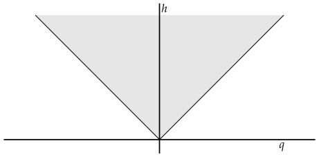
Figure 18: Allowed states in the $h$-$q$ plane (shaded). Small representations occur on the boundary.

This idea plays a key role throughout supersymmetry. Now note that if we have a small representation and we make continuous changes in the parameters in the Hamiltonian, the energy of the states cannot change—it must stay at $h=|q|$ because to move to $h>|q|$ we would need four states.

The $N=4$ supersymmetry algebra has regular representations of $2^{8}$ states and small representations of $2^{4}$ states. The masses, electric and magnetic charges satisfy the Bogomolńyi-Witten-Olive bound [98]

$$M^{2}\geq v^{2}(Q_{e}^{2}+Q_{m}^{2}),$$ (3.5.13)

where $v$ is the symmetry-breaking expectation value (this is for a single $U(1)$ group). Small representations saturate the bound. In the perturbative, small $g$, theory, both the charged gauge bosons and the stable monopole solutions are in small representations, and moreover one finds the same spin spectrum in each case. Now vary the coupling $g$. Small representations have to stay small, and saturate the bound, so by the time we get to $g^{\prime}=\sqrt{4\pi}/g$ the spin and mass spectrum is the same as we started with but with electric and magnetic charges interchanged.

I have never known what to make of this—is it a simple consequence of supersymmetry restricted to the Bogomolńyi sector, or is it evidence for a duality of the full theory? I have always been skeptical, again because the duality seems to lead to a mess at the Lagrangian level. However, notice that while the BWO bound determines the allowed spectrum of small representations, but it is a further non-trivial fact that the actual spectrum found is dual [99]. The final bit of evidence for duality, the long-ranged force, is also a consequence of the BWO bound.

Everything I have just said was known before 1980 for the electric-magnetic duality. Sen recently observed that the $SL(2,Z)$ would have additional implications ([93] and references therein). In particular, it requires stable states of monopole charge $n_{2}$ greater than one, which must appear as bound states of the $n_{2}=1$ states. Some of these have now been found [100]. Recently, long papers by Seiberg and Witten [101], [102] and Vafa and Witten [103] on $N=2$ and $N=4$ supersymmetric gauge theories have appeared, which seem to present further evidence for duality, though I have not absorbed these. All of this evidence refers in a sense only to the Bogomolńyi sector of the spectrum, but so much is accumulating that it is harder to believe that it is not a symmetry of the full spectrum.

Thus far the discussion has involved only field theory, $N=4$ supersymmetric Yang-Mills. For the heterotic string compactified on a six-torus (that is, $\mu=4,\ldots 9$ periodic) the low energy theory contains $N=4$ Yang-Mills, and the conjecture is that this string theory also is self-dual [92], [93]. The circumstantial evidence is of the same type as the above. Let me just note a few important differences. The coupling constant $g^{2}$ is now a field, being proportional to $e^{\Phi}$. But so also is the topological angle $\theta$: it is proportional to the axion field $a$ obtained from the antisymmetric tensor.
Exercise: Show that for the two-index potential $B_{\mu\nu}$, if one interchanges the Bianchi identity for the field strength (vanishing curl) with the equation of motion (vanishing gradient), in four dimensions one obtains a massless scalar field. Show that in ten dimensions one obtains a 7-index antisymmetric tensor field strength which is the curl of a 6-index potential, and which is invariant under a 5-index gauge transformation.
The low energy field theory for the dilaton, axion, and gauge fields, and their supersymmetric partners, is $SL(2,Z)$ invariant.

The other difference is that the BWO sector, which in the field theory case consisted of a few small representations, is now very much larger, with infinite numbers of electrically charged string states and magnetically charged soliton states, of various types. The duality of the allowed states follows from supersymmetry as above, but duality of the actual spectrum implies much more, including ‘stringy’ monopoles which involve fields not in the low energy effective field theory. At this point it is much less clear whether the actual spectrum is $S$-dual. Incidentally, Sen has also argued that $S$-duality, like $R$-duality, must be a gauge symmetry in string theory.

Finally, another conjecture is that string theory is dual to a theory of fundamental five-dimensional objects (ref. [104] and further references in ref. [93]). The evidence is of the same type as the above—duality of the low energy field theory, and interchange of the spectra of ‘fundamental’ objects and solitonic ones. These arguments are made even though it is not known if it is possible to quantize the fundamental five-brane—the world-sheet theory is a six-dimensional field theory and so non-renormalizable. They are made on the basis of presumed low-energy field theory of the five-brane (it couples naturally to a six-index antisymmetric tensor gauge field; see the above exercise), on its classical soliton solutions, on scaling arguments based on the world-sheet and spacetime theories, and on the possible winding states of a five-dimensional object. An interesting connection between this and $S$-duality is that

$$S_{\rm string}=(\mbox{5-brane $\to$ string})(R_{\mbox{\scriptsize 5-brane}})(\mbox{string $\to$ 5-brane})\ ,$$ (3.5.14)

so string/5-brane duality would imply $S$-duality, given the more straightforward $R$-duality.

4 String Field Theory or Not String Field Theory

Thus far, we have defined string theory only through its perturbation expansion, the analog of Volume One of Bjorken and Drell. Now we would like to find Volume Two. We know that in field theory there are many important phenomena that cannot be seen in perturbation theory, and string theory will have all of these and probably more. Also, we have found that string theory contains an enormous amount of spacetime gauge invariance, in the form of spacetime Ward identities satisfied by the scattering amplitudes. But again, we know from Yang-Mills theory and general relativity that this is a very clumsy way to think about spacetime gauge invariance. These theories of course have a geometrical interpretation which is essential to understanding the physics, and which is disguised in the perturbation theory but is evident when they are written as field theories. So it seems that we should try something similar in string theory, to introduce some sort of string field $\Psi$, to find an action with the appropriate gauge symmetries, and then to recover the perturbation theory from a gauge-fixed path integral. This section consists of a few assorted remarks about this idea, focusing first on some very attractive features, and then on some indications that it may not be quite the right thing to do.

4.1 String Field Theory

A closed string field will create or destroy a string along some closed curve in spacetime, so it is a functional $\Psi[X]$ of such paths. An open string field will be a functional of open curves. In the earlier discussion, the closed and open string wavefunctions $\psi[X]$ were similarly functionals of the configuration of the string in spacetime, so this is like second quantization, ‘promoting’ the one-particle wavefunction to an operator (or, in the path integral formalism, to a variable of integration). It turns out that things work very much more nicely if one first goes to the BRST-invariant form of the theory, and then second quantizes [105], [106]. In this form the wavefunction also includes the state of the ghosts. Since the $b$ and $c$ ghosts are conjugate, we can for example regard $b$ as the momentum and $c$ are the coordinate, so the wavefunction would be a functional $\psi[X,c]$, and the corresponding field a functional $\Psi[X,c]$. Actually, it is still convenient to use the bra-ket notation, writing the string field as $|\Psi\rangle$, which is just the abstract notation for the functional $\Psi[X,c]=\langle X,c|\Psi\rangle$. We would have to use a different notation for the states of the theory, something like $|\Phi)$. That is, $|\Phi)$ is a state with any number of strings, and $\Psi[X,c]$ or $|\Psi\rangle$ act as an operators on these states.

We can think about this another way by expanding the functional $|\Psi\rangle$ in terms of a complete set of such functionals. For the open string, for example,

$$|\Psi\rangle=\int\frac{d^{26}k}{(2\pi)^{26}}\,\Bigl{\{}T(k)|0,k\rangle+iA_{\mu}(k)\alpha_{-1}^{\mu}|0,k\rangle+B(k)b_{-1}c_{0}|0,k\rangle+\ldots\,\Bigr{\}}.$$ (4.1.1)

The functions $T(k)$, $A_{\mu}(k)$, $B(k),\ldots$ or their Fourier transforms $T(X)$, $A_{\mu}(X)$, $B(X),\ldots$ are the arbitrary coefficients in the expansion. There is an obvious interpretation of $T(X)$ as the spacetime tachyon field and $A_{\mu}(X)$ as the spacetime gauge field, while $B(X)$ will turn out to be an auxiliary field.

Now we need an invariance principle. Since wavefunctions $Q_{\rm B}|\chi\rangle$ are equivalent to zero, the natural guess is

$$|\Psi\rangle\ \to\ |\Psi\rangle+Q_{\rm B}|\Upsilon\rangle$$ (4.1.2)

for any $|\Upsilon\rangle$. Taking

$$|\Upsilon\rangle=\int\frac{d^{26}k}{(2\pi)^{26}}\,\Bigl{\{}\lambda(k)b_{-1}|0,k\rangle+\ldots\,\Bigr{\}},$$ (4.1.3)

(so that $Q_{\rm B}|\Upsilon\rangle$ has the same ghost number as $|\Psi\rangle$) one finds from the expansion (2.5.23) of $Q_{\rm B}$ that the invariance (4.1.2) becomes

$$\delta A_{\mu}(X)=-2\partial_{\mu}\lambda(X)$$ (4.1.4)

which is indeed the linearized gauge invariance of electromagnetism.

There is an obvious free field equation,

$$Q_{\rm B}|\Psi\rangle\ =0,$$ (4.1.5)

which is invariant under (4.1.2) because $Q_{\rm B}^{2}=0$. In components, this becomes

$$\partial^{2}T(X)=-\frac{1}{2}T(X),\qquad B(X)=-\partial_{\mu}A^{\mu}(X)$$

$$\partial^{2}A_{\mu}(X)=-\partial_{\mu}B(X)=\partial_{\mu}\partial_{\nu}A^{\nu}(X).$$ (4.1.6)

We obtain the appropriate Klein-Gordon equation for the tachyon and the gauge-invariant free Maxwell equation for $A_{\mu}$. Note that the field equation (4.1.5) has the same form as the physical state condition which earlier gave us the mass-shell conditions. The one difference is that we required $b_{0}$ to annihilate physical states, which at this level leads to $B(X)=0$ and so $\partial^{2}A_{\mu}(X)=0$. So the $b_{0}$ condition is a stringy generalization of Feynman gauge.

We can readily write down an invariant free action as well. It is simply

$$S_{\rm open}=\frac{1}{2}\langle\Psi|Q_{\rm B}|\Psi\rangle.$$ (4.1.7)

The ghost number works out so that the action for the fields (4.1.1) is non-zero. Writing the inner product in terms of the path integral on the disk, the vertex operators ${\cal V}_{\Psi}$ each have ghost number 1, as does $Q_{\rm B}$, adding up to 3 as required by the same calculation (1.9.4) as on the sphere. Not surprisingly, the action for $A_{\mu}$ is the free Maxwell action, after $B$ is integrated out. We have used the bilinear inner product $\langle\ |\ \rangle$, but in fact the string field must satisfy a reality condition

$$\langle\Psi|=\langle\!\langle\Psi|.$$ (4.1.8)

This is necessary for unitarity, generalizing the familiar fact that the metric and Yang-Mills fields must be real.

This all seems very beautiful to me. The familiar spacetime gauge invariance is embedded as the lowest component of a much larger symmetry acting on all higher levels of the string, and the BRST formalism allows this to be done in an extremely compact and elegant way. In fact, the action (4.1.7) has the same structure as the Abelian Chern-Simons action $\int d^{3}X\,AdA$ [106], where $Q_{\rm B}$ is analogous to the exterior derivative $d$: note that both are nilpotent. Incidentally, the components of other ghost number, not written in the expansion (4.1.1), just play the role of Fadeev-Popov ghosts for the spacetime gauge symmetry after the gauge is fixed, and one obtains a BRST-invariant string field theory. To be precise, there are several complications relative to the earlier discussion of BRST symmetry on the world-sheet, so a generalization of BRST, the Batalin-Vilkovisky formalism, emerges [107].

This all generalizes to the closed string, with a slight complication. It is necessary to impose conditions $(b_{0}-\tilde{b}_{0})|\Psi\rangle=(L_{0}-\tilde{L}_{0})|\Psi\rangle=0$ on the closed string field and on the gauge parameter $|\Upsilon\rangle$, and the action is

$$S_{\rm closed}=\frac{1}{2}\langle\Psi|(c_{0}-\tilde{c}_{0})Q_{\rm B}|\Psi\rangle.$$ (4.1.9)

The ghost number is then correct. The invariance (4.1.2) is now an infinite-dimensional generalization of linearized coordinate invariance.

Now the question is whether we can find an appropriate nonlinear generalization of the string gauge symmetry and action. Let us transform this into a related question. After gauge fixing, the path integral over the string field can be expanded perturbatively in terms of Feynman diagrams built from string propagators and vertices. Is it possible to represent the amplitudes, which were described earlier in terms of a sum over world-sheets, in this way?

I am going to make a distinction here between what I will call an effective string field theory and a bare string field theory, and describe the former first. What I am call an effective string theory is described in ref. [68]. It is always possible by brute force to write the string amplitudes in terms of Feynman diagrams. Let us introduce an arbitrary three-closed-string vertex, as depicted in fig. 19a. Figure 19b shows a four-string amplitude built from two such vertices.

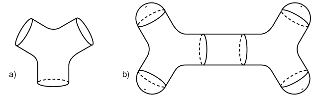
Figure 19: a) Three-string vertex. b) Four string amplitude.

The propagators are cylinders, with lengths integrated from zero to infinity (generalizing the Schwinger representation of the propagator in field theory). There are three such graphs, from the three channels. Now recall from the Virasoro-Shapiro amplitude (2.8.1) that this amplitude is supposed to be given by an integral of one vertex operator position $z_{4}$ over the complex plane, the other three operators being fixed. The graphs of fig. 19b cover three round regions centered on the three fixed positions, fig. 20a, but this inevitably leaves a region between uncovered.

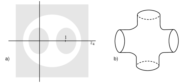
Figure 20: a) Graph of fig. 19b covers three round regions in the complex plane. b) Four-string vertex needed to cover unshaded region in fig. 20a.

So it is necessary to introduce a four-string vertex as shown in fig. 20b. An integration over shape in included in the definition of the vertex so as to cover exactly the missing region of fig. 20a. Going on to higher amplitudes, one must further introduce $n$-string vertices for all $n$. At tree level the vertices have the topology of spheres with $n$ holes. However, when one goes on to loop amplitudes, the tree level action again does not cover moduli space, so it is necessary to add additional vertices containing internal loops. This procedure can be carried out iteratively, and in the end the full perturbation series is written in terms of Feynman graphs. Ref. [68] gives an explicit construction of one possible set of vertices. All of this can also be applied to theories of open plus closed strings.

Now one can work backwards, writing the $n$-string vertex as a term in the action with a product of $n$ string fields. The resulting action does indeed have a non-linear generalization of the string gauge symmetry. This is not surprising for the following reason. In the discussion of spacetime Ward identities in section 2.7, I emphasized that these would hold if and only if the integration ran over the correct moduli space. The iterative construction of the vertices does this, so the spacetime Ward identities hold and a corresponding invariance should be present in the action. The condition that moduli space be properly covered is equivalent to a set of identities for the vertices, and these same identities imply the nonlinear invariance of the action [68].

4.2 Not String Field Theory

I have called the above construction an effective string field theory because it is very similar to a Wilsonian effective field theory. The long-distance physics is explicitly represented, while the short-distance physics is already integrated out. (A similar analogy was made in refs. [109]). In particular, we have seen that long-distance propagation in spacetime, producing the poles in string amplitudes, comes from long cylinders or strips at the boundaries of moduli space. In the effective string field theory, the vertices include an integration over moduli, but only an interior region of moduli space, as in the example of fig. 20. The degenerating cylinders appear explicitly as propagators. On the other hand, we will see at two points later on that stringy physics comes from the interior of moduli space, which are hidden inside the vertices.

Effective string field theory is very useful for some purposes. By describing explicitly the boundaries of moduli space it is a useful tool for demonstrating the finiteness and unitarity of string perturbation theory—see the discussion at the end of section 2. But it would not seem to be the right tool for studying nonperturbative string theory, since the stringy physics is already integrated out. Can we do better? For the open string we certainly can [106]. The simple Witten vertex shown in fig. 21, in which three open strings are joined by gluing their halves together in pairs, exactly covers moduli space.

Figure 21: Witten vertex for three open strings.

The interacting action thus has a nonlinear generalization of the string gauge invariance, and has the same structure as the non-Abelian Chern-Simons action. I will call this a ‘bare string theory,’ since the action has a closed form without corrections from all orders in the loop expansion.

The perturbative formulations of open and closed string theories were quite parallel. For example, the spectrum of the closed string was essentially the tensor product of two copies of the open string spectrum. But now we run into a real asymmetry, for there does not seem to be any covariant closed string field theory simpler than the effective theory that I described earlier. The existence of $n$-point tree level interactions would not have been surprising, since general relativity is non-polynomial while Yang-Mills theory is polynomial. But the fact that the action receives corrections from all orders in the quantum loop expansion means that a great deal of non-trivial physics is already integrated out.

There is another, rather remarkable, asymmetry between open and closed strings. The Witten open string theory covers the moduli space of Riemann surface with boundaries. But as I have emphasized at the end of section 2.5, this will include processes with intermediate closed strings. The simplest example of this is in fig. 22, the one loop vacuum amplitude, with one propagator and no vertices.

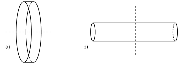
Figure 22: a) Annulus at large $t$. Cutting on dashed line gives an open string pair. b) Annulus at small $t$. Cutting on dashed line gives a single closed string.

This has a modulus $t$, the ratio of the circumference to the length, which runs from $0$ to $\infty$. For large $t$, fig. 22a, this looks like a vacuum fluctuation consisting of a pair of open strings. But for small $t$, fig. 22b, it looks like a single closed string appearing and then disappearing. Indeed, the string graph contains both processes. The same thing happens at for higher order open string amplitudes. While we can think of the Witten theory as a path integral over open string fields, it contains the full open plus closed string physics [110].

It is not clear what the logical relation is between the closed and open strings here. It is not that the closed strings are bound states of open strings—there are no interactions in fig. 22. In some sense the closed strings are singular configurations of the open string field. Siegel has suggested recently that the relationship is similar to bosonization, though I do not grasp all his arguments [111]. Perhaps the lesson is that open string field theory is all we need, with the closed string emerging as in fig. 22. This idea was pursued for a while, but it is not clear where to go with it [112]. There is also the difficulty that the most promising theory, the heterotic string, does not have an open string version.

The graph in fig. 22 is the same as the one-loop vacuum amplitude in field theory, with $t$ the Schwinger parameter, and it corresponds to summing $\frac{1}{2}\omega$ times the spacetime volume over all open string modes. It is interesting to contrast this with closed string theory. Figure 22 is obtained by taking an open string propagator, a strip of length/width$=t$, gluing the ends and integrating over $t$. The analogous construction in closed string theory would be to take a cylinder, gluing the ends, and integrating over lengths and also twist angles. This would correspond to integrating over tori, with the modulus $\tau$ running over the full region Re$(\tau)<\frac{1}{2}$, Im$(\tau)>0$. This is not the integration region, fig. 6, for closed string theory. So the closed string vacuum amplitude is not given by summing $\frac{1}{2}\omega$ over closed string frequencies, a strong indication that closed string theory is not a field theory [113]. The open string vacuum amplitude is given by summing $\frac{1}{2}\omega$ over open string frequencies, though it includes also the closed string process of fig. 22b.

There is one more important non-field-theoretic property of closed strings, having to do with the large-order behavior of the perturbation series. Consider a quantum field theory where the coupling constant $g$ appears only as an overall factor $g^{-2}$ in the action, so that $g^{2}$ is the loop counting parameter. Rather generally, the large order behavior of the perturbation series $\sum_{h=0}^{\infty}g^{2h}T_{h}$ (reviewed in ref. [114]) is

$$T_{h}\ \sim\ h!h^{A}C^{-h}$$ (4.2.1)

with $A$ and $C$ constants. The dominant factor here is the factorial. Generically this arises simply because the number of Feynman graphs with $h$ loops is of order $h!$—if one cuts off the momentum integrations in the IR and UV the propagator and vertex factors just enter into the constants $A$ and $C$. The perturbation series is thus divergent. The ratio of successive terms is

$$\frac{g^{2h}T_{h}}{g^{2h-2}T_{h-1}}\ \sim\ hC^{-1}g^{2},$$ (4.2.2)

so the smallest term is for $\tilde{h}\sim Cg^{-2}$. From Stirling’s approximation,

$$A_{\tilde{h}}\sim e^{-C/g^{2}}.$$ (4.2.3)

This is the smallest term, so represents the maximum accuracy of perturbation theory as an asymptotic series. Indeed, many non-perturbative effects, effects which do not occur at any order of perturbation theory, are of this magnitude, including confinement, chiral symmetry breaking, supersymmetry breaking in supersymmetric gauge theories, instantons, even BCS superconductivity.

Open string theory is much the same [115]. The Witten field theory represents moduli space as a sum of Feynman graphs, so the factorial growth of the number of graphs implies a factorial volume of moduli space. The integrand can be bounded in the interior of moduli space, so again barring infrared divergences the same estimate (4.2.1) holds, and nonperturbative effects of order $e^{-C/g_{\rm o}^{2}}$ are expected.

The same argument does not apply to closed string theory, because the effective string field theory has complicated vertices containing integrals over moduli space. Shenker estimates the large order behavior as follows [116]. He uses the fact that Witten’s open string field theory generates the amplitudes of the full open plus closed string theory. He then argues that the purely closed-string amplitudes are a non-negligible portion of the full amplitudes, so that the perturbation theory for them grows as rapidly. Nonperturbative effects are then of order

$$e^{-C/g_{\rm o}^{2}}=e^{-C/g_{\rm c}}.$$ (4.2.4)

In terms of the closed string perturbation theory, this translates into large order behavior proportional to $(2h)!$, as had been discovered in the matrix models.

These $e^{-C/g_{\rm c}}$ effects have no analog in field theory, and their nature is not known. We will see what they are in the matrix model, but it has been hard to guess how to generalize the result. At small $g_{\rm c}$ these stringy effects are larger than the familiar and important $e^{-C/g_{\rm c}^{2}}$ nonperturbative effects in the low energy field theory. Moreover, they are likely to involve phenomena which are unique to string theory. Of all the things I am covering in these lectures, this is the one where I most wanted to be able to say something new. I have made one observation [117], which is that if one includes boundaries with Dirichlet conditions, $X^{\mu}=$constant, these act as instantons but with a weight of the desired form $e^{-C/g_{\rm c}}$. The conjecture is that the stringy nonperturbative effects make their appearance as a sum over various kinds of boundaries; I am trying to test this in the matrix model.

In lieu of anything solid to say, let me make a conjecture: that closed string field theory is simply wrong nonperturbatively, and that closed strings themselves are collective excitations of some other degrees of freedom, in terms of which the theory should be formulated. Let me list some evidence for this.

• The rapid growth of perturbation theory, suggesting that the perturbative description is rather far from the exact formulation.

• The fact that closed string field theory does not seem to work, except as an effective theory with the stringy physics integrated out. Note that the rapid growth of perturbation theory implies that the interior of moduli space, the part which does not look like Feynman graphs and is integrated into the vertices, is very large.

• The appearance of closed strings in open string field theory.

• Matrix models, where closed strings are collective (bosonized) excitations of free fermions.

• The closed string is almost the product of right- and left-moving theories, suggesting that it might be useful to regard it as a bound state of right-moving and left-moving strings. In the flat space theory, there are two things which glue the two sides together. The first is the equality of the zero modes eigenvalues, $\alpha_{0}=\tilde{\alpha}_{0}$. The second is the global structure of moduli space. Locally, the moduli space has a natural complex structure corresponding to the right-left separation—for example, the modulus $\tau$ of the torus appears as $\tau L_{0}-\bar{\tau}\tilde{L}_{0}$. But the region of integration is not any sort of product.

• Too much gauge symmetry. Here I am being contrary, since earlier I told you that it was wonderful that string theory embedded the spacetime gauge symmetries in a much larger structure. There I was following the usual particle theory paradigm that local symmetry is holy, and that as one goes to higher and more fundamental energies one expects to see more and more of it, as in $SU(3)\times U(1)\in SU(3)\times SU(2)\times U(1)\in SU(5)$ of the Standard Model and GUTS. But this need not be the case. As I have tried to emphasize, gauge symmetry is just a useful redundancy, and there are examples where one emerges at low energy even though there is no sign of it in the underlying theory. The familiar example from particle theory is the $CP(n)$ sigma model [118]. In condensed matter physics, this has been proposed to occur in theories of strongly coupled electrons, where the electron separates into a ‘spinon’ and ‘holon,’

  $$\psi_{e}(x,t)=\psi_{s}(x,t)\phi(x,t).$$ (4.2.5)

  This decomposition is redundant, the transformation

  $$\psi^{\prime}_{s}(x,t)=e^{i\lambda(x,t)}\psi_{s}(x,t),\qquad\phi^{\prime}(x,t)=e^{-i\lambda(x,t)}\phi(x,t)$$ (4.2.6)

  leaving the physical field, the electron, invariant. It is plausible that under some conditions this redundancy is elevated to a dynamical symmetry (for a review see ref. [119]). As far as I know there is no reason in principle that this cannot happen. So perhaps the short distance theory, rather than exhibiting an enormous gauge symmetry, should be formulated entirely in terms of invariants.

  Recall from the discussion in section 3.4 that one way to distinguish a useless from a useful redundancy is to see whether the fields transform inhomogeneously. The string gauge symmetry is

  $$|\Psi\rangle\ \to\ |\Psi\rangle+Q_{\rm B}|\Upsilon\rangle+O(|\Psi\rangle)$$ (4.2.7)

  The linear term is as before, eq. (4.1.2). We do not know the higher terms in any simple form but we do not need them, because it is precisely the term $Q_{\rm B}|\Upsilon\rangle$, of zeroth order in $|\Psi\rangle$, that is relevant here. If this vanishes (at least for some momentum), the gauge symmetry is real. So we are looking for solutions of

  $$Q_{\rm B}|\Upsilon\rangle=0.$$ (4.2.8)

  This looks like the physical state condition, but it is different because the $|\Upsilon\rangle$ have ghost number one less than the states, so it is a different cohomology. In fact, the only solutions for a flat background are $\Upsilon=\partial X^{\mu}\tilde{c}$ or $c\bar{\partial}X^{\mu}$, which are just the translations, so the only ‘real’ gauge symmetries are those of the graviton and antisymmetric tensor. But this need not be conclusive—there are other backgrounds where other parts of the string gauge symmetry are unbroken, as we will see in section 5, so it may be that it is useful to keep the full redundancy.

• The observation that holes in the world-sheet naturally give effects of order $e^{-C/g_{\rm c}}$ [117], suggesting a breakdown of the world-sheet.

This is the set of ideas I play with, though it does not yet add up to anything coherent.

The idea that we should look for more fundamental degrees of freedom in string theory was put forward in ref. [121], in a study of the high-temperature behavior of string theory. This discusses a number of other non-field-theoretic properties of closed strings, and also suggests breakdown of the world-sheet by way of holes. Another idea [122], [123] is that the string should be thought of as a collection of bits; the string picture breaks down when the density of bits becomes large. It may be that these ideas are connected, holes appearing in the world-sheet because neighboring bits unbind.

4.3 High Energy and Temperature

In particle physics the traditional way to find out what things are made of is to bang them together. I will briefly describe three different high-energy regimes, each of which gives a different picture. We might hope that in one limit or another the theory will simplify enough to allow us to go beyond perturbation theory.

The first limit is scattering at high center-of-mass energy, $E=s^{1/2}$, and fixed angle. This is where Rutherford found the atomic nucleus, and where SLAC found the partonic constituents of hadrons, quarks and gluons. In relativistic field theory this process probes distances of order $E^{-1}$. We have already seen in the tree-level Virasoro-Shapiro amplitude that the amplitude is very soft in this limit. To get further insight[124] consider the path integral over $X^{\mu}$ from which it was obtained,

$$\int[dX]\,e^{-S_{\rm P}+i\sum_{i=1}^{4}k_{i}\cdot X(\sigma_{i})}\ ,$$ (4.3.1)

the second term in the exponent being from the tachyon vertex operators. The limit is essentially obtained by scaling up the $k_{i}$ uniformly. The action $S_{\rm P}$ is quadratic in $X$, so the path integral is determined by a saddle point $X^{\mu}_{\rm cl}\ \propto\ E$, and the amplitude is $e^{-O(E^{2})}$. This same saddle point dominates if the tachyons are replaced with other states of the string; in particular, the masses of the external states drop out in the limit. Also the $z_{4}$ integral in the resulting amplitude (2.8.2) is dominated by a saddle point, at

$$z_{4}=\frac{k_{1}\cdot k_{4}}{(k_{1}+k_{2})\cdot k_{4}}\ .$$ (4.3.2)

Note that this is in the interior of moduli space, another example of the idea that stringy behavior comes from the interior.

In contrast to field theory, the size of the interaction region grows with energy [124]. Combining the low energy field theoretic behavior with this high energy result, the effective uncertainty is

$${\mit\Delta}X\ \sim\ \frac{1}{E}+\alpha^{\prime}E.$$ (4.3.3)

This is further evidence for an effective minimum distance in string theory, as found earlier from duality. It appears that the string can carry only of order one string unit of energy per unit length, so to transfer a much larger energy $E$ many bits are needed—the effective number of partons is proportional to the energy.

Gross and Mende were able to find the dominant saddle point at every order of perturbation theory. It is just an $n$-fold cover of the tree-level saddle point, scaled by a factor $n^{-1}$, with $n-1=h$ being the number of loops. The exponential in the scattering amplitude (2.8.4) is suppressed by $n$,

$$c_{n}e^{-sf(\theta)/n}$$ (4.3.4)

so at large $s$ high orders dominate. This can be interpreted in terms of dividing the scattering into $n$ softer scatterings of angle $\theta/n$. There has been some discussion of the summation of this series [125], and of a large symmetry in the high energy limit [126], assuming that it is correct simply to sum the leading behavior from each order. It is interesting to contrast this with the earlier discussion of the large-order behavior. The amplitude (4.3.4) comes from a single saddle point in moduli space, so is unrelated to the large volume noted earlier. However, it is enhanced by the kinematics and actually grows much faster than the volume of moduli space, $c_{n}$ being proportional to $(9h)!$.

The second limit is soft scattering, high energy and small angle, holding fixed the momentum transfer $q\sim(-t)^{1/2}$. Whereas the hard scattering is an occasional rare process where many bits of string move together, the soft scattering is a picture of the typical string configuration. From Stirling’s approximation, the Virasoro-Shapiro amplitude is of order

$$A_{\rm VS}\ \sim\ s^{2+t}t^{-1}=\frac{s^{2}}{t}e^{-q^{2}(\ln s)}.$$ (4.3.5)

This is the gravitational amplitude $s^{2}/t$ modified by a form-factor which corresponds to an object with a size of order $\sqrt{\ln E}$ [128]. There is another way to see this same result. Let us calculate the root-mean-square size of the string ground state. The mode expansion gives

$$\langle 0|(X^{1}(\sigma)-\overline{X^{1}})^{2}|0\rangle\ =\ \sum_{m=1}^{\infty}\frac{1}{m^{2}}\langle 0|(\alpha_{m}\alpha_{-m}+\tilde{\alpha}_{m}\tilde{\alpha}_{-m})|0\rangle\ =2\sum_{m=1}^{\infty}\frac{1}{m}.$$ (4.3.6)

This is divergent but has no direct physical significance. A measurement on a time-scale $\delta t$ is sensitive only up to modes of frequency less than $\delta t^{-1}$, essentially $m\,\delta t<1$. So the log divergence becomes $\ln(\delta t^{-1})$, and the size is the square root of this [128]. This agrees with the form factor, where the soft scattering probes time scales $\delta t\sim{1/E}$.

Just as the hard scattering (4.3.3) is interpreted as a stringy uncertainty principle, Susskind interprets this root-log-$E$ growth as a stringy Lorentz transformation, transverse sizes not being constant as in classical physics. A similar calculation shows that the longitudinal size of the string goes to a constant of order the string scale, not the usual contraction as $1/E$.

The square root of a logarithm is a very slow function, and ordinarily would be of little importance. But there is one situation where enormous boosts are encountered—a black hole. From Strominger and Verlinde you have heard two very different points of view on whether short distance physics, such as string theory, can be relevant to the information problem. What makes this so controversial is that in a black hole there are no large local invariants, such as would ordinarily be needed for the low energy effective field theory to break down, but there is a very large nonlocal invariant, the relative boost between an infalling and an asymptotic observer. The external observer ‘sees’ the infalling observer slow down and sit forever (or until the hole decays) on the horizon. One tick of the infalling clock takes longer and longer as seen from the outside, the ratio going as $e^{t/4M}$ with $M$ the mass of the hole and $t$ the time measured by the external observer. So the external observer is seeing the internal motion of infalling strings slowed down, a fixed time scale $\delta t_{\rm ext}$ corresponding to a time interval $e^{-t/4M}\delta t_{\rm ext}$ for the infalling object. As time goes on, the external observer ‘sees’ more and more of the modes of the string, and it appears to grow, as

$$\sqrt{\ln(e^{t/4M}\delta t_{\rm ext}^{-1})}\ \propto t^{1/2}.$$ (4.3.7)

Before the black hole evaporates, the string grows to macroscopic sizes, and low energy field theory no longer applies. Also, because of its longitudinal behavior the string, rather than contracting closer and closer to the horizon, remains a finite thickness above it. Again, this would have a profound effect on the Hawking radiation.

However, I have put ‘sees’ in quotes, because to see one needs light, and the black hole is black. Of course there is Hawking radiation, but the conventional wisdom is that this is produced outside the horizon—the relevant modes are in their ground states near the horizon—and so cannot reveal all of the marvelous things that the string is doing, and the string physics is irrelevant. At least, I have not been able to imagine a real dynamical calculation which shows the stringy effects to be relevant. But this picture of the essentially diffusive growth of the string is very simple and appealing [129], and the stringy properties do dovetail very nicely with what would be needed to solve the information problem. It may be that the low energy field theoretic treatment is internally consistent but not correct, because the large nonlocal invariant makes string theory important even before the low energy field theory breaks down internally due to a large local invariant. This would be a satisfying resolution of the various points of view; the problem is to find the right calculation!

The previous limits involved two strings, each in a state of low excitation but with large center of mass energy. The final limit I will discuss is that of a single string in a very high state of excitation. The density of single-string states per unit energy $n(\varepsilon)$ is related to the free energy in the noninteracting limit,

$$\beta F(\beta)=\int_{0}^{\infty}d\varepsilon\,n(\varepsilon)e^{-\beta\varepsilon},$$ (4.3.8)

where I have used the fact that $e^{-\beta\varepsilon}$ will be much less than 1 for the relevant states. The density of states grows exponentially, as $e^{\beta_{\rm c}\varepsilon}$, so the integral converges at low temperature but diverges at $\beta<\beta_{\rm c}$. It is tempting to interpret this as a transition (the Hagedorn transition) to a phase where the conjectured fundamental degrees of freedom will be evident. As yet, there is little understanding of the high-temperature phase.

There is a large literature on this subject, but here I just wish to note that there is a very simple picture of the typical high-energy string state, which gives a surprisingly good quantitative account of the density of states [130]-[133]. First let me tell you more precisely what the density of states is. In the limit $\varepsilon\to\infty$, at fixed volume, it is

$$n(\varepsilon)=\frac{1}{\varepsilon}e^{\beta_{\rm c}\varepsilon}.$$ (4.3.9)

This is true for any finite volume spatial background, such as a torus, or a group manifold. If instead one takes the linear size to infinity faster than $\varepsilon^{1/2}$, one finds

$$n(\varepsilon)=\frac{V}{\varepsilon^{(1+D)/2}}e^{\beta_{\rm c}\varepsilon}.$$ (4.3.10)

where $D$ is the number of spacetime dimensions and $V$ the volume.

The results (4.3.9) and (4.3.10) follow if one assumes that the typical highly excited string is a random walk, with its length proportional to its energy. First, the exponential factor comes from the fact that the number of steps is proportional to the length, with a choice to be made at each step. The Hagedorn transition thus arises from a competition between the energy and entropy of a long string. The power-law prefactor is important for the details of the transition. In the density (4.3.10), the factor of $V$ is counts the number of places a random walk might start. We must then divide by the typical volume of the random walk, because we can make a closed string only if the final point and initial point coincide; this gives a factor of $\varepsilon^{(1-D)/2}$. Finally, this overcounts by a factor of the length of the string, since we can start at any point along the closed string, so we need an additional factor of $\varepsilon^{-1}$, giving the result (4.3.10). In finite volume, the random walk will eventually fill the space so that its volume is just $V$, giving instead (4.3.9). Remarkably, the density of states is completely independent of the size and shape of the space in this limit. With such a simple picture of the free theory we might hope that the interacting theory will be tractable.

5 Matrix Models

5.1 $D=2$ String Theory

Returning to the theme of my introduction, one of the things I learned from Wilson’s lecture is the extent to which he was influenced by the pion-nucleon static model. This is an essentially one-dimensional free pion field in interaction with a static nucleon with some internal states. In spite of having only one interacting degree of freedom, this model has the essence of quantum field theory, a nontrivial renormalization group flow.

String theory has an enormous number of degrees of freedom and a rather rigid structure. It is not easy to find models which are simple enough to deal with and yet retain the essential features of the theory. In the previous section we mentioned various high energy limits where things seem to simplify a bit, but as yet it has not been possible to do anything beyond perturbation theory. The one limit which has turned out to be solvable is the limit of small numbers of spacetime dimensions, $1\leq D\leq 2$ (for reviews see refs. [134], [135]).

A simple solution to the background field equations (3.1.2) for arbitrary $D$ is [136]

$$G_{\mu\nu}=\eta_{\mu\nu},\qquad B_{\mu\nu}=0,\qquad\Phi=QX^{1}/2$$ (5.1.1)

with

$$Q^{2}=\frac{26-D}{3}.$$ (5.1.2)

The field equations (3.1.2) were derived in world-sheet perturbation theory and are generally true only when the gradients of the background fields are small, but the solution (5.1.1) is a special case because the path integral remains gaussian. In fact, we have already constructed the CFT. On a flat world-sheet the world-sheet action reduces to the ordinary free $X^{\mu}$, but with energy-momentum tensor as in eq. (1.6.1),

$$T=-\frac{1}{2}:\!\partial X^{\mu}\partial X_{\mu}\!:-\frac{1}{2}Q\partial^{2}X^{1}$$ (5.1.3)

giving $c=D+3Q^{2}=26$.

What is the physics of this background? Recall that $e^{\Phi}$ plays the role of the string coupling, so the coupling is position-dependent, as $e^{QX^{1}/2}$. For $X^{1}\to-\infty$ the coupling goes to zero, but for $X^{1}\to\infty$ the coupling diverges and string perturbation theory breaks down. Adding a tachyon background produces a theory in which string perturbation theory is valid. The vertex operator $e^{\alpha X^{1}}$ has weight

$$h=\tilde{h}=\frac{-(2\alpha-Q)^{2}+Q^{2}}{8},$$ (5.1.4)

so for $Q^{2}\geq 8$, which is $D\leq 2$, there are two positive real solutions to the mass-shell condition $h=\tilde{h}=1$. It is the lesser, $\alpha_{1}\leq Q/2$, which is appropriate,

$$T(X^{1})\sim e^{\alpha_{1}X^{1}}\ .$$ (5.1.5)

Adding this to the action gives

$$S=\frac{1}{8\pi}\int d^{2}\sigma\,\Bigl{\{}\sqrt{g}g^{ab}\eta_{\mu\nu}\partial_{a}X^{\mu}\partial_{b}X^{\nu}+Q\sqrt{g}RX^{1}+\mu e^{\alpha X^{1}}\Bigr{\}}.$$ (5.1.6)

The $X^{1}$ action is the Liouville theory. The tachyon background (‘Liouville wall’) suppresses the path integral at large $X^{1}$ where the coupling is strong, the exponential factor in the acion dominating the linear factor from the growth of the coupling.

This string theory is solvable at $D=1$ or 2, or for one Liouville dimension plus a minimal model (recall from eq. (1.9.11) that the central charge counts the number of degrees of freedom, so a minimal model is like less than one whole dimension). I will concentrate on $D=2$, which has the most physics. As we have discussed, the physical state conditions remove two sets of oscillators, leaving in this case none. Only the center of mass motion, the tachyon, remains. For real momentum the vertex operator (1.6.5) is $e^{ik\cdot X+QX^{1}/2}$. The factor $e^{QX^{1}/2}$ we now recognize as the string coupling, which multiplies the tachyon wavefunction. The weight, given that $Q^{2}=8$ in $D=2$, is $1+\frac{1}{2}k^{2}$, so the mass-shell condition is $k^{2}=0$. The tachyon is misnamed in $D=2$: it is massless!
Exercise: Show in the same way that $M^{2}=-\frac{1}{12}(D-2)$ in general $D$. This can be interpreted as the negative Casimir energy of the $D-2$ transverse modes.

The theory thus reduces to a massless scalar field moving in one time and one space dimension. The spatial dimension is not translation-invariant. Rather, the coupling goes to zero at $X^{1}\to-\infty$, and grows with $X^{1}$ until we reach the ‘Liouville wall,’ the tachyon background which cuts off further propagation [139].

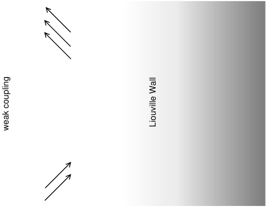
Figure 23: Two dimensional spacetime with dilaton and tachyon backgrounds. The S-matrix describes transitions from a state with $m$ incoming tachyons to a state with $n$ outgoing tachyons.

The basic physics is to throw tachyons in from $-\infty$; near the wall they interact with each other and reflect back to $-\infty$. This is about as rich as throwing pions at a static nucleon. Just as the latter proved to contain the essence of field theory, the $D=2$ string has taught us at least one important lesson about the full theory, the existence of the large nonperturbative effects. I will review the solution, what has been learned, and what more we might hope to learn.

5.2 The $D=1$ Matrix Model

The method by which the $D=2$ string theory was solved is completely orthogonal to what we have discussed thus far. It begins with the quantum mechanics of an $N\times N$ Hermitean matrix M(t) [140]. The action is

$$S=\beta N\int dt\,\biggl{\{}\frac{1}{2}{\rm Tr}\,(\dot{\bf M}^{2})+{\rm Tr}\,V({\bf M})\biggr{\}}\ .$$ (5.2.1)

Here $\beta$ is a parameter and $V$ a general potential. You have already heard about this sort of thing from one or more of Ambjorn, Ginsparg, and Moore, so I will go through the solution without dwelling too much on the details. A graph with given numbers of propagators $P$, vertices $V$, and loops $L$ will depends on $\beta$ and $N$ as $\beta^{n_{V}-n_{P}}N^{n_{V}-n_{P}+n_{L}}=\beta^{-n_{L}}(\beta N)^{\chi},$ where $\chi$ is Euler number of the surface we get by filling in the index loops in the graphs. Thus, for any amplitude

$$A(\beta,N)=\sum_{n_{L},\chi}A_{n_{L},\chi}\beta^{-n_{L}}(\beta N)^{\chi},$$ (5.2.2)

where $A_{n_{L},\chi}$ is the contribution from graphs with given numbers of loops and given topology. The Hamiltonian is

$$H=-\frac{1}{2\beta N}\sum_{i,j}\frac{\partial}{\partial M_{ij}}\frac{\partial}{\partial M_{ji}}+\beta N{\rm Tr}\,V({\bf M}).$$ (5.2.3)

The action is invariant under the $U(N)$ which takes ${\bf M}\to{\bf UMU}^{-1}$. We will only be interested in singlet states—when one cuts open a graph, the states will always be traces of M’s, and so invariant. A singlet state is a function only of the eigenvalues $\lambda_{i}$. Acting on such a state one finds (use first and second order perturbation theory to take the derivatives of eigenvalues)

$$H{\Psi}(\lambda) = \sum_{k}\biggl{\{}-\frac{1}{2\beta N}\frac{\partial^{2}}{\partial\lambda_{k}^{2}}+\frac{1}{\beta N}\sum_{l\neq k}\frac{1}{\lambda_{l}-\lambda_{k}}\frac{\partial}{\partial\lambda_{k}}+\beta NV(\lambda_{k})\biggr{\}}{\Psi}(\lambda)$$ (5.2.4)

$$= \Delta^{-1}(\lambda)H^{\prime}\Delta(\lambda){\Psi}(\lambda)$$

where

$$H^{\prime}=\beta N\sum_{k}\biggl{\{}-\frac{1}{2\beta^{2}N^{2}}\frac{\partial^{2}}{\partial\lambda_{k}^{2}}+V(\lambda_{k})\biggr{\}},$$ (5.2.5)

and $\Delta(\lambda)=\prod_{k<l}(\lambda_{k}-\lambda_{l})$. We will absorb the factor of $\Delta$ into the wavefunction and work with ${\Upsilon}(\lambda)=\Delta(\lambda){\Psi}(\lambda)$. The inner product works out in a simple way: after the angular integrations,

$$\int d^{N^{2}}{\bf M}\,{\Psi}^{*}(\lambda){\Psi}(\lambda)\ \propto\int d^{N}\lambda\,{\Upsilon}^{*}(\lambda){\Upsilon}(\lambda),$$ (5.2.6)

so ${\Upsilon}$ is the probability amplitude for the eigenvalues.

The Hamiltonian (5.2.5) describes $N$ decoupled coordinates. The factor of $\Delta$ in $\Upsilon$ makes the wavefunction antisymmetric, so this is a system of $N$ free fermions [140]. It can also be written in terms of a second-quantized spinless fermion field $\zeta(\lambda)$,

$$H^{\prime}=\beta N\int d\lambda\,\biggl{\{}\frac{1}{2\beta^{2}N^{2}}\partial_{\lambda}\zeta^{\dagger}\partial_{\lambda}\zeta+V(\lambda)\zeta^{\dagger}\zeta\biggr{\}}\ .$$ (5.2.7)

From the $N$-dependence (5.2.2), the $N\to\infty$ limit is dominated by graphs of spherical topology. This limit is easily taken in the free-fermion form. Although we set the original $\hbar$ to 1, we see that if we define $H^{\prime}=\beta NH^{\prime\prime}$ then $\beta N$ appears in $H^{\prime\prime}$ precisely the way $1/\hbar$ appears in the Hamiltonian for nonrelativistic quantum mechanics. The $N\to\infty$ limit at fixed $\beta$ is then classical. Each fermion occupies a volume $2\pi$‘$\hbar$’ = $2\pi/\beta N$ in phase space. Levels with single-particle energy $E^{\prime\prime}=\frac{1}{2}p^{2}+V<\varepsilon_{F}$ are filled. The total number of fermions is $N$, so

$$\frac{1}{\beta}=\frac{N}{\beta N}=\int\frac{dp\,d\lambda}{2\pi}\,\theta\biggl{(}\varepsilon_{F}-\frac{p^{2}}{2}-V(\lambda)\biggr{)}\ .$$ (5.2.8)

Now let us, to be specific, take

$$V(\lambda)=\frac{1}{4}\lambda^{2}(2-\lambda)^{2}.$$ (5.2.9)

For large $\beta$, the phase space integral (5.2.8) is small, and the fermions sit near the quadratic minimum at $\lambda=0$. One finds $\varepsilon_{F}\sim\beta^{-1/2}$. There are no fermions in the second minimum at $\lambda=2$: the Feynman rules represent perturbation theory around ${\bf M}=0$, and the second minimum is invisible in perturbation theory. Figure 24 shows the potential, with occupied states shaded.

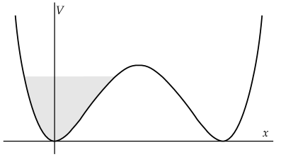
Figure 24: Potential energy for fermions, with filled states shaded.

As $\beta$ decreases, the occupied phase space volume grows. At some critical value $\beta_{\rm c}$ the Fermi level reaches the local maximum, $\varepsilon_{\rm c}=\frac{1}{4}$ at $\lambda=1$, and there is a phase transition (see [141] for a review). Quantities such as

$$\langle 0|H^{\prime}|0\rangle=N^{2}\int\frac{dp\,d\lambda}{2\pi}\,\left\{\frac{p^{2}}{2}-V(\lambda)\right\}\theta\biggl{(}\varepsilon_{F}-\frac{p^{2}}{2}-V(\lambda)\biggr{)}$$ (5.2.10)

are analytic for $\beta>\beta_{\rm c}$ and have a singularity at $\beta_{\rm c}$.
Exercise: Show that in terms of $\delta=\varepsilon_{\rm c}-\varepsilon_{F}$,

$$\beta-\beta_{\rm c}\sim\delta\ln\delta,\qquad\langle 0|H|0\rangle\sim\delta^{2}\ln\delta,$$ (5.2.11)

up to terms analytic in $\delta$ [142]. This takes a bit of care, because the analytic terms in these two quantities are larger than the singular ones, though they are irrelevant because they do not come from large surfaces. Show from this that the contribution $A_{n_{L},2}$ defined in eq. (5.2.2) goes as $n_{L}^{-3}\beta_{\rm c}^{n_{L}}$ for $\langle 0|H|0\rangle$ at large $n_{L}$.

Now recall, from the counting (5.2.2), that $\beta^{-1}$ is the loop-counting parameter for perturbation theory. So for a potential with a local maximum, the perturbation series has a finite radius of convergence, diverging beyond $\beta^{-1}=\beta_{\rm c}^{-1}$. The non-analyticity in $\beta-\beta_{\rm c}$ then arises from large orders of perturbation theory, large graphs. Here is where the connection with string theory comes in. Assign a length $a$ to each propagator. As $n_{L}\to\infty$, one might hope to take $a\to 0$ in such a way that the sum over graphs approaches a sum over smooth surfaces, so the critical behavior in $\beta-\beta_{\rm c}$ is given by a string theory [142]. There are other possibilities—the typical graph might instead look like a branched polymer—which can arise in the limit of large discrete surfaces. But in this case we are lucky, and the limit is a string theory. We can verify this by comparing various quantities that can be calculated both in the matrix model and in the continuum theory, and then use the matrix model to do many calculations that we cannot yet do in the continuum.

We have taken the large $N$ limit, so we have only surfaces of spherical topology. Thus, the ground state energy (5.2.10) is explicitly $O(N^{2})$. We can do better [143]. Let us take $N\to\infty$ and $\beta\to\beta_{\rm c}$ together, holding fixed

$$\overline{\mu}=\beta N(\varepsilon_{\rm c}-\varepsilon_{F}).$$ (5.2.12)

This is the double scaling limit. Since $(\beta N)^{-1}$ plays the role of $\hbar$, the splitting between fermionic levels is of order $1/\beta N$, and the ratio of this splitting to the distance $\varepsilon_{\rm c}-\varepsilon_{F}$ from the critical Fermi level remains constant. The splitting thus remains non-negligible in the double scaling limit. Since the splitting is a $1/N$ effect, vanishing in the spherical limit, the double scaling limit is keeping nontrivial contributions from all topologies, with Euler number $\chi$ being weighted by $\overline{\mu}^{\chi}$. That is, each additional handle brings in $\overline{\mu}^{-2}$.

The double-scaling limit is easily taken directly in the Hamiltonian. Define

$$\lambda-1=(\beta N)^{-1/2}x,\qquad\zeta=(\beta N)^{1/4}\psi.$$ (5.2.13)

Thus, for fixed $x$, the eigenvalue $\lambda$ approaches the local maximum as $N\to\infty$. Only the quadratic behavior near the maximum survives in this limit. The Hamiltonian becomes

$$H^{\prime}-\beta N\varepsilon_{F}=\int dx\,\biggl{\{}\frac{1}{2}\partial_{x}\psi^{\dagger}\partial_{x}\psi-\frac{x^{2}}{2}\psi^{\dagger}\psi+\overline{\mu}\psi^{\dagger}\psi\biggr{\}}\ .$$ (5.2.14)

The result is simply a Fermi sea in an inverted oscillator potential.

5.3 Matrix Model $\leftrightarrow$ String

What do we expect for the continuum string theory corresponding to this critical behavior? The number of links separating two vertices gives a measure of distance, so we expect a world-sheet metric $g_{ab}(\sigma)$. And, each vertex occurs at some time $t$, so this should become a world-sheet field $t(\sigma)$ in the continuum limit. The most relevant action for these fields is

$$S_{nc}=\int d^{2}\sigma\,\sqrt{g}\biggl{\{}-c_{1}g_{ab}\partial_{a}t\partial_{b}t+c_{2}+c_{3}R\biggr{\}}\ .$$ (5.3.1)

There is no reason to expect Weyl-invariance. Consequently the world-sheet cosmological constant term $c_{2}$ has been included. We have earlier discussed briefly the world-sheet theories without Weyl invariance. We can go to the conformal gauge

$$g_{ab}(\sigma)=e^{\varphi(\sigma)}\hat{g}_{ab}(\sigma),$$ (5.3.2)

in which the metric is reduced to the degree of freedom $\varphi(\sigma)$. Taking into account the Fadeev-Popov determinant and the Weyl anomaly from the $t$-integration, the action becomes [50]

$$\int d^{2}\sigma\,\sqrt{\hat{g}}\biggl{\{}-c_{1}\hat{g}_{ab}\partial_{a}t\partial_{b}t+c_{2}e^{\varphi}+c_{3}\hat{R}+\frac{25}{96\pi}(\hat{g}^{ab}\partial_{a}\varphi\partial b\varphi+2\hat{R}\varphi)\biggr{\}}\ .$$ (5.3.3)

We started with one spacetime dimension, but as we have noted the Weyl factor in the metric behaves very much like an extra embedding dimension. So we can think of this as a non-critical string in one dimension with metric $g_{ab}$, or a critical string in two dimensions with metric $\hat{g}_{ab}$. The former is appropriate if one is interested in two-dimensional quantum gravity on the world-sheet; the latter is appropriate if one is interested in two-dimensional string theory in the embedding space. Ambjorn’s lectures focus on the former, and mine on the latter. Although the theories are the same, one tends to ask different questions in the two cases. In the former case, the focus is on various measures of the world-sheet geometry, while in the latter it is on scattering processes in the embedding space.

Comparing the result (5.3.3) with our expectation (5.1.6), we see precisely the same terms with $\varphi\propto X^{1}$, but the coefficients cannot be made to match up—the ‘25’ needs to be ‘24’ and the exponent in the cosmological term is wrong. This has a simple explanation. The derivation of (5.3.3) implicitly defined the $\varphi$ path integral using the metric $g_{ab}$, while the latter used the metric $\hat{g}_{ab}$, and the difference is accounted for by the corresponding renormalization of the measure [145]. This is presumed now to be well-understood [146] and is not something I want to dwell on, so I use the action in the form (5.1.6) with the relative normalization of $X^{0}$ (in the string theory) and $t$ (in the matrix model) yet to be determined.

To summarize, we expect that the free fermion theory (5.2.14) is equivalent to $D=2$ string theory in the dilaton and tachyon background (5.1.5). In the string theory we had tachyons bouncing off a Liouville wall. In the matrix model we have fermions bouncing off the inverted harmonic potential. So things look very close, the string theory being a bosonization of the matrix model.

Let us carry out the bosonization in detail [147]-[149]. In the classical limit we can describe the collective motions of the fermions in terms of a time dependent Fermi surface, separating the filled and empty phase space regions. Fermions on the surface on the surface move freely in the inverted harmonic potential,

$$D_{t}p=x,\qquad D_{t}x=p,$$ (5.3.4)

where $D_{t}$ denotes the co-moving derivative, following one phase-space point on the surface. The solution is

$$p=-a\sinh(t-b),\qquad x=-a\cosh(t-b)$$ (5.3.5)

with integration constants $a$ and $b$. In contrast, the position $p$ of the Fermi surface at fixed $x$ satisfies $\partial_{t}p|_{x}=D_{t}p-\partial_{x}p|_{t}D_{t}x=x-\partial_{x}p|_{t}p$. For perturbations that are not too large (and we will return to these later), the Fermi sea can be described by the positions of its upper lower surfaces at each time, $p_{\pm}(x,t)$, and each satisfies

$$\partial_{t}p_{\pm}(x,t)=x-p_{\pm}(x,t)\partial_{x}p_{\pm}(x,t).$$ (5.3.6)

For example, from the Hamiltonian (5.2.14) it follows that the static Fermi level is given by $\frac{1}{2}(p^{2}-x^{2})+\overline{\mu}=0$ or

$$p_{\pm}(x)_{\rm static}=\pm\sqrt{x^{2}-2\overline{\mu}}\ ,$$ (5.3.7)

which satisfies the equation of motion (5.3.6).

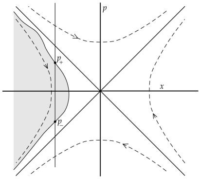
Figure 25: Fermi sea: filled states in the $x$-$p$ plane are shaded. The state of the sea is given by the upper and lower surfaces $p_{\pm}(x,t)$, shown at a representative value of $x$. Points on the Fermi surface move along hyperbolic orbits.

The Hamiltonian in terms of $p_{\pm}$ is obtained by integrating the single-particle energy over the Fermi sea,

$$H^{\prime} = \frac{1}{2\pi}\int_{-\infty}^{\infty}dx\int_{p_{-}}^{p_{+}}dp\,\frac{1}{2}(p^{2}-x^{2})$$ (5.3.8)

$$= \frac{1}{2\pi}\int_{-\infty}^{\infty}dx\,\biggl{\{}\frac{1}{6}(p_{+}^{3}-p_{-}^{3})-\frac{x^{2}}{2}(p_{+}-p_{-})\biggr{\}}\ .$$

Also, from the equation of motion and the Hamiltonian one can deduce the commutator

$$[p_{\pm}(x),p_{\pm}(y)]=-2\pi i\partial_{x}\delta(x-y),\qquad[p_{+}(x),p_{-}(y)]=0.$$ (5.3.9)

To write this in terms of a massless scalar, define the coordinate $q=-\ln(-x)$, which runs from $-\infty$ to $\infty$ as $x$ runs from $-\infty$ to 0, and define a scalar field $\overline{\cal S}(q,t)$.

$$p_{\pm}(x,t) = \mp x\pm\frac{1}{x}\epsilon_{\pm}(q,t)$$

$$\pi^{-1/2}\epsilon_{\pm}(q,t) = \pm\overline{\pi}_{\cal S}(q,t)-\partial_{q}\overline{\cal S}(q,t).$$ (5.3.10)

The bar is to distinguish this scalar from a slightly different one to appear later. The Hamiltonian takes the form

$$H^{\prime}=\frac{1}{2}\int_{-\infty}^{\infty}dq\Bigl{\{}\overline{\pi}_{\cal S}^{2}+(\partial_{q}\overline{\cal S})^{2}+e^{2q}O(\overline{\cal S}^{3})\Bigr{\}}.$$ (5.3.11)

The quadratic part is the canonically normalized free scalar Hamiltonian; the equation of motion is $(\partial_{t}^{2}-\partial_{q}^{2})\overline{\cal S}=e^{2q}O(\overline{\cal S}^{2})$.

The collective motion of the matrix model fermions has the same qualitative behavior as the $D=2$ string theory discussed earlier. Asymptotically it is a free massless scalar, with interactions that grow exponentially. In the string theory, strings are reflected from the Liouville wall before the coupling diverges, while in the matrix model they are reflected from the end of the eigenvalue distribution. Thus, our guess that the $D=2$ critical string describes the critical behavior of the $D=1$ matrix model appears to be correct. The coupling goes as $e^{\sqrt{2}X^{1}}$ in string theory and $e^{2q}$ in the matrix model, which determines the relative normalization of these. Also, the velocity is 1 in both the $q$-$t$ and $X^{1}$-$X^{0}$ planes, so we have

$$X^{1}\sim q\sqrt{2},\qquad X^{0}\sim t\sqrt{2}.$$ (5.3.12)

We had earlier concluded that $\overline{\mu}^{-2}$ is the loop-counting parameter, which would make $\overline{\mu}^{-1}$ the three-string coupling. We can now check this. From the static distribution (5.3.7), the turning point in the eigenvalue distribution is at $x_{t}\ \propto\ \overline{\mu}^{1/2}$. The dominant interactions occur at the Liouville wall $x_{t}$, where the coupling $g_{\rm s}$ goes as $e^{2q_{t}}=x_{t}^{-2}\ \propto\ \overline{\mu}^{-1}$ as expected. More detailed comparisons are possible as well, and in particular the relation between the string coordinate $X^{1}$ and the matrix model eigenvalue $q$ is more subtle than the scaling argument (5.3.12) suggests. We will return to this, after discussing some general issues.

Two asides before we go on. First, it is interesting to contrast the bosonization we have just done with relativistic bosonization. The latter relates the collective motion of a free massless relativistic fermion to a free massless boson. The difference is that the relativistic fermion has a linear dispersion relation, $\omega\ \propto\ k$, while the matrix model fermions have $\omega\ \propto\ k^{2}$. Looking at the Hamiltonian, we see that the cubic scalar interaction comes from the term quadratic in momentum. We can think about this as follows. Relativistic fermions have no dispersion, the velocity $\partial_{k}\omega$ being a constant. A collective pulse propagates without changing its shape. The matrix model fermions have a $k$-dependent velocity, so that a pulse deforms as it propagates. This translates into interactions among the bosons.

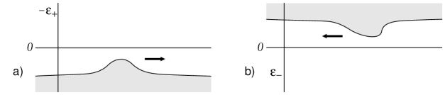
Figure 26: a) Incoming pulse on top of the static Fermi sea. For clarity the variable $-\epsilon_{+}(q,t)$ is shown. b) Later outgoing pulse, with shape distorted by dispersion. Fermions closer to $|p|=|x|$ travel more deeply into the potential and take longer to return.

Second, the endpoint of the distribution, where $p_{+}-p_{-}\to 0$, causes difficulties. At this point the dynamics is determined not by the Hamiltonian but by the constraint that the fermion density $p_{+}-p_{-}$ be positive. Further, perturbation theory in the collective Hamiltonian suffers various divergences at the endpoint, which need to be appropriately regulated. It is sometimes useful to work with the Fourier transformed fermion $\tilde{\psi}(p,t)$, in terms of which the Hamiltonian looks almost the same [150],

$$H^{\prime}-\beta N\varepsilon_{F}=\int dp\,\biggl{\{}-\frac{1}{2}\partial_{p}\tilde{\psi}^{\dagger}\tilde{\partial}_{p}\psi+\frac{p^{2}}{2}\tilde{\psi}^{\dagger}\tilde{\psi}+\overline{\mu}\tilde{\psi}^{\dagger}\tilde{\psi}\biggr{\}}\ .$$ (5.3.13)

The collective motion can now be described in terms of the surface $x(p,t)$. In this variable the sea has only an upper edge, and there is no endpoint to worry about.

5.4 General Issues

So what does one learn from all this? The object of study is the amplitude for $m$ incoming strings of energies $\omega_{1},\ldots,\omega_{m}$ to evolve into $n$ outgoing strings of energies $\omega^{\prime}_{1},\ldots,\omega^{\prime}_{n}$. The matrix model allows the exact calculation of these amplitudes [151]. One starts with the incoming strings, translates into an incoming fermion state using bosonization (asymptotically we have noted that the bosons become free, so one can use the familiar relativistic bosonization), evolve the free fermions in the inverted harmonic potential, and then translate back using bosonization. The final closed form from combining all these steps is a little complicated, but for given $m$ and $n$ one can follow through the steps and find the exact answer, without resorting to expansion in the closed string coupling $\overline{\mu}^{-1}$. The same calculations remain exceedingly hard within the continuum string theory. One must in principle carry out the path integral over $X^{\mu}$, integrate over moduli space, and sum over genus. Even the first of these is nontrivial, because the path integral is not gaussian, due to the tachyon background. The path integral on the sphere has been carried out using difficult analytic arguments, and for some amplitudes by taking advantage of the large symmetry of the problem, to be developed later.

Undoubtedly the main physical lesson learned thus far is the discovery of the large non-perturbative effects, which as we have seen turned out to be a general feature of string theory [116]. In the matrix model, there is an obvious nonperturbative process, the tunneling of a single fermion through the potential barrier. Now we have to consider an issue that we have ignored so far, namely what is going on on the other side of the barrier. There are many possibilities—that the other side is empty (so the state we are considering is unstable); that it is filled to the same Fermi level as the first well; that the potential is modified, say by an infinite barrier at some $x\geq 0$. None of these would change the perturbation theory, so they represent a nonperturbative ambiguity. Later we will examine the problem of the nonperturbative definition of the theory, but for now we will just use this ambiguity to estimate the inaccuracy of perturbation theory. The fermion tunneling amplitude is $e^{-B}$ with $B$ given in the WKB approximation by

$$B=\int_{-\sqrt{2\overline{\mu}}}^{\sqrt{2\overline{\mu}}}dx\,\sqrt{2\overline{\mu}-x^{2}}=\pi\overline{\mu}.$$ (5.4.1)

So the tunneling amplitude is indeed $e^{-O(\overline{\mu})}=e^{-O(g_{\rm s}^{-1})}$. From the discussion in section 4, one would expect this to be associated with a $(2h)!$ growth of the perturbation theory. This growth is indeed found when the amplitudes are expanded in powers of $\overline{\mu}^{-2}$ [143].

In this case one can see what the nonperturbative effect associated with the large order behavior is, namely single-fermion tunneling. The matrix model is an example of this picture in which the strings are collective excitations of something simpler, the free fermions. The bosonic collective Hamiltonian can presumably be used to generate all orders of perturbation theory, but it is not at all clear that one can make sense of it non-perturbatively. The description of the single-fermion tunneling in terms of the collective Hamiltonian is extremely clumsy and ad hoc. More generally, the collective description seems to break down near the end of the eigenvalue distribution, or for processes involving interference between two edges of the Fermi surface. For example, the raising operators of the $\overline{\cal S}$ field create a fermion-hole pair. An operator with momentum greater than $p_{+}-p_{-}$ tries to create a hole below the lower edge $p_{-}$ of the Fermi sea, which is impossible. So the algebra of the bosonic raising and lowering operators—the enumeration of states—breaks down. A very similar thing happens in the case of $D=2$ Yang-Mills theory. The string representation can be obtained as a bosonization of a non-relativistic free fermion representation just as here, and again the enumeration of string states breaks down non-perturbatively, when the number of boxes in a Young tableau column exceeds $N$.

One would of course like to use this to get some insight into the nature of the nonperturbative effects and of the hypothetical fundamental degrees of freedom in higher dimensions. One can try looking at limits in the higher dimensional theory as I have discussed, but another avenue is to try to make as explicit as possible the connection between the free fermion picture and the string picture here in the $D=2$ theory. At present the connection is quite roundabout, going through the matrix model and double scaling limit. In fact, the connection is rather subtle. The string theory tachyon is related in an obvious way to the collective motion of the fermions, but in fact there is more in the string theory. The graviton-dilaton sector of the $D=2$ string theory is the same as the dilaton gravity theories discussed by Strominger and Verlinde. So although there is no propagating graviton or dilaton, there are still physical effects from gravity, including a black hole solution. These are not evident in the matrix model. It is important to clarify this, both to develop the matrix model $\leftrightarrow$ string connection, and because the gravitational effects are of interest in their own right.

We have been discussing the $D=1$ (also called $c=1$) matrix model. The $D=0$ model, based on a single matrix ${\bf M}$ without time, leads in a similar way to the $D=1$ string (pure world-sheet gravity = one Liouville dimension). Multi-matrix models ${\bf M}_{i}$ lead to $0<c<1$, the minimal models plus a Liouville dimension. Also, fine-tuned multicritical points in the $D=0$ matrix model lead to non-unitary minimal models plus the Liouville dimension. The extension to $c>1$ is problematic. The matrix model can no longer be reduced to eigenvalues, and no solution is known. Also, as we have noted the tachyon really is tachyonic beyond $D>2$, so the vacuum is unstable and presumably does not correspond to an attractive fixed point of the discrete theory.

Even at $D\leq 2$ it would be useful to have a greater variety of models, so as to get some perspective. The matrix model can be generalized to open plus closed strings [154] (a different approach is given in ref. [155]). This reduces to a theory of interacting fermions. It is similar to the $U(N)$ Calogero-Sutherland model recently considered by Haldane and others, but has not been solved. Even short of a full solution, it would be useful to understand in the classical limit the connection between the collective excitations and the open and closed strings. Another extension is spacetime supersymmetry. Supersymmetry breaking is after all one of the most important non-perturbative phenomenon in string theory; spacetime supersymmetry would also help with the tachyon instability of the $c>1$ string. There is nothing useful here yet. A straightforward supersymmetrization of the $D=1$ matrix model exists and has a double-scaling limit [156]. But Shyamoli Chaudhuri and I have recently shown that the naive world-sheet theory is not conformally invariant, and the theory flows to some exotic fixed point that does not seem to be connected with the string physics that is of interest [157].

To conclude these lectures, I will first develop some details of the tree-level scattering amplitudes. I will then discuss the gravitational physics of the $D=2$ string, including the black hole solution, as well as the generalization to higher string levels. Finally, I look for the corresponding physics in the matrix model. I show how gravitational physics emerges in the weak field limit, then look at physics in strong fields—an (as yet unsuccessful) search for the black hole solution, some exotic strong-field physics that arises in the matrix model, and the nonperturbative ambiguity.

5.5 Tree-Level Scattering

Consider a small incoming pulse on top of the static solution $p_{\pm,\rm static}$, eq. (5.3.7). As we have discussed, dispersion changes the shape of the pulse: higher points on the pulse travel deeper into the potential and emerge later. Let us work this out at the classical level. The equation of motion (5.3.4) implies that

$$v=(-x-p)e^{-t},\qquad w=(-x+p)e^{t}$$ (5.5.1)

are constant for a particle moving in the inverted harmonic potential. Then so also are the integrals

$$v_{mn}=e^{(n-m)t}\int_{F-F_{0}}\frac{dp\,dx}{2\pi}\,(-x-p)^{m}(-x+p)^{n}.$$ (5.5.2)

The integral runs over the Fermi sea $F$, with the integral over the static Fermi sea $F_{0}$ subtracted, so this will converge for a pulse of finite width. Evaluating this in the limits $t\to-\infty$ and $t\to\infty$ relates the incoming and outgoing pulses. As $t\to-\infty$ points approach the line $p=-x$, so

$$v\to e^{q-t}\epsilon_{+}(q-t),\qquad w\to 2e^{-q+t}\ .$$ (5.5.3)

I have used the expansion (5.3), with the free field equation of motion $\epsilon_{+}(q,t)\sim\epsilon_{+}(q-t)$ for the incoming wave. Similarly, as $t\to\infty$,

$$v\to 2e^{-q-t},\qquad w\to e^{q+t}\epsilon_{-}(q+t)$$ (5.5.4)

with $\epsilon_{-}$ the outgoing wave. Thus,

$$v_{mn} = \frac{2^{n}}{2\pi(m+1)}\int_{-\infty}^{\infty}dt\,e^{(n-m)(t-q)}\Bigl{\{}(\epsilon_{+}(t-q))^{m+1}-\overline{\mu}^{m+1}\Bigr{\}}$$ (5.5.5)

$$= \frac{2^{m}}{2\pi(n+1)}\int_{-\infty}^{\infty}dt\,e^{(n-m)(t+q)}\Bigl{\{}(\epsilon_{-}(t+q))^{n+1}-\overline{\mu}^{n+1}\Bigr{\}}.$$

Applying this for $m=0$, $n=i\omega$ gives the Fourier transform of the incoming wave as a nonlinear function of the outgoing wave [158], [159]. Expanding around the static background, $\epsilon_{\pm}(q_{\mp})=\overline{\mu}+\delta\epsilon_{\pm}(q_{\mp})$, gives

$$\int_{-\infty}^{\infty}dq_{-}\,e^{i\omega q_{-}}\delta\epsilon_{+}(q_{-})=(2\overline{\mu})^{i\omega}\int_{-\infty}^{\infty}dq_{+}\,e^{-i\omega q_{+}}\sum_{k=1}^{\infty}\frac{\overline{\mu}^{1-k}}{k!}\frac{\Gamma(1+i\omega)}{\Gamma(2-k+i\omega)}\delta\epsilon_{+}(q_{+})^{k}.$$ (5.5.6)

In terms of the Fourier modes,

$$\epsilon_{\pm}(q_{\mp})=\overline{\mu}+\frac{1}{\sqrt{2\pi}}\int_{-\infty}^{\infty}d\omega\,\overline{\alpha}_{\pm}(\omega)e^{\pm i\omega q_{\mp}}$$ (5.5.7)

this becomes

$$\overline{\alpha}_{+}(\omega) = \sum_{k=1}^{\infty}\frac{(\sqrt{2\pi}\overline{\mu})^{1-k}}{k!}\frac{\Gamma(1+i\omega)}{\Gamma(2-k+i\omega)}$$

$$\qquad\int d\omega_{1}\ldots d\omega_{k}\,\overline{\alpha}_{-}(\omega_{1})\ldots\overline{\alpha}_{-}(\omega_{k})\delta(\omega_{1}+\ldots+\omega_{k}-\omega)\ .$$

It is a useful fact that classical scattering is the same as tree level quantum scattering. The quantum operators satisfy the same equation of motion as the classical field, so the solution (5.5) also holds, except that we would have to be careful about operator ordering. But commutators are of order $\hbar$ and so do not matter to leading order. The modes have been normalized to satisfy

$$[\overline{\alpha}_{\pm}(\omega),\overline{\alpha}_{\pm}(\omega^{\prime})]=-2\pi\omega\delta(\omega-\omega^{\prime}).$$ (5.5.9)

Defining the in-states

$$|\omega_{1},\ldots,\omega_{n};\overline{\rm in}\rangle=\overline{\alpha}_{+}(\omega_{1})\ldots\overline{\alpha}_{+}(\omega_{n})|0\rangle,\qquad\omega_{i}>0,$$ (5.5.10)

and similarly for the out-states, the classical S-matrix (5.5) plus the canonical commutator (5.5.9) give the tree level S-matrix. For example, the $1\to n$ amplitude is [158]

$$\langle\omega_{1},\ldots,\omega_{n};\overline{\rm out}|\omega;\overline{\rm in}\rangle=\left(\frac{\sqrt{2\pi}}{\overline{\mu}}\right)^{n-1}\frac{\Gamma(1+i\omega)}{\Gamma(2-n+i\omega)}2\pi\delta(\omega_{1}+\ldots+\omega_{n}-\omega).$$ (5.5.11)

This same calculation can also be done by string methods, but only with great effort and ingenuity. The main complication is the exponential term in the string action, from the tachyon background. Far from the Liouville wall this is small, so for so-called ‘bulk’ processes which happen far away from the wall we can use the free action or at least expand in powers of $\overline{\mu}$. (One can think about using wavepackets to separate out the bulk processes, as I will describe later). We then have a free-field string calculation of the type that gave the Virasoro-Shapiro amplitude. In $D>2$ this reduces to $\Gamma$-functions only for four particles, but in $D=2$ the kinematic restrictions make it possible to evaluate for any number. Also, an analytic continuation makes it possible to deduce the full amplitude from the bulk amplitude. The result is almost the same as the matrix model result (5.5.11). That is, comparison of the string and matrix model S-matrices shows that the latter is related to the former by [160]-[162].

$$\alpha_{+}(\omega) = \frac{\Gamma(i\omega)}{\Gamma(-i\omega)}\overline{\alpha}_{+}(\omega)$$

$$\alpha_{-}(\omega) = \frac{\Gamma(-i\omega)}{\Gamma(i\omega)}\overline{\alpha}_{-}(\omega).$$ (5.5.12)

The ratio of gamma functions, known as the ‘leg pole’ factor, is a pure phase for real frequencies, so this is a unitary transformation on the states. Such a redefinition is not surprising. The matrix model gives a discrete approximation to the local vertex operator $e^{iq\cdot X+X^{1}\sqrt{2}}$. One expects to find a renormalization for any such cutoff construction. Following this line of thought one can, purely within the matrix model, deduce the poles and zeroes of the leg pole factor.

I will not pursue this, but simply take the leg pole factor from the comparison of amplitudes. Although a pure phase, it will play an essential role soon.

5.6 Spacetime Gravity in the $D=2$ String

Now let us take a closer look at the graviton, dilaton, and antisymmetric tensor states in the $D=2$ string,

$$|e,k\rangle=e_{\mu\nu}\alpha^{\mu}_{-1}\tilde{\alpha}^{\nu}_{-1}|0,k\rangle.$$ (5.6.1)

Recall from section 1.6 the Virasoro generators

$$L_{0} = \frac{1}{2}k^{2}+\frac{a^{2}}{2}+\sum_{n=1}^{\infty}\alpha_{-n}\cdot\alpha_{n}$$

$$L_{m} = \frac{1}{2}\sum_{n=-\infty}^{\infty}\alpha_{n}\cdot\alpha_{m-n}+i(m+1)a\cdot\alpha_{m},\qquad m\neq 0,$$ (5.6.2)

where $a^{\mu}=(0,\sqrt{2})$. Also recall $\alpha_{0}=k^{\mu}-ia^{\mu}$. Acting on the state (5.6.1), the physical state conditions become (we use the convenient OCQ form)

$$L_{0},\tilde{L}_{0}: k^{2}=-a^{2}$$

$$L_{1},\tilde{L}_{1}: (k+ia)^{\mu}e_{\mu\nu}=(k+ia)^{\nu}e_{\mu\nu}=0.$$ (5.6.3)

Also, acting with $L_{-1}$ on the state $f_{\mu}\alpha^{\mu}_{-1}|0,k\rangle$ and with $\tilde{L}_{-1}$ on $\tilde{f}_{\nu}\tilde{\alpha}^{\nu}_{-1}|0,k\rangle$ we find the following spurious states

$$\mbox{spurious:}\qquad e_{\mu\nu}=(k-ia)_{\mu}\tilde{f}_{\nu}+f_{\mu}(k-ia)_{\nu}\$$ (5.6.4)

for any $f$, $\tilde{f}$.

The $L_{1}$ and $\tilde{L}_{1}$ conditions require $e_{\mu\nu}$ to be orthogonal to $k+ia$ on both indices, or $e_{\mu\nu}=n_{\mu}n_{\nu}$ where $n_{\mu}$ is in the one-dimensional space orthogonal to $k+ia$. The $L_{0}$ conditions gives $(k+ia)\cdot(k-ia)=0$, so $n\ \propto\ k-ia$. But this means that $e_{\mu\nu}$ is spurious, so there are no ‘observable’ states.

This is correct at generic momenta but breaks down at special points [161]. If $k=-ia$, the $L_{1}$ and $\tilde{L}_{1}$ conditions are empty. States with polarizations proportional to $a^{\mu}$ are null in this case, so we can remove the spacelike polarizations and be left with the observable state

$$\alpha^{0}_{-1}\tilde{\alpha}^{0}_{-1}|0,-ia\rangle\ .$$ (5.6.5)

If $k=ia$ the spurious state vanishes. The physical state condition requires $e_{\mu\nu}$ to be orthogonal to $a^{\mu}$, so the observable state is

$$\alpha^{0}_{-1}\tilde{\alpha}^{0}_{-1}|0,+ia\rangle\ .$$ (5.6.6)

The corresponding vertex operators are respectively

$$:\!\partial X^{0}\bar{\partial}X^{0}e^{2\sqrt{2}X^{1}}\!:\ ,\qquad:\!\partial X^{0}\bar{\partial}X^{0}\!:\ .$$ (5.6.7)

What does this mean physically? The absence of observable states at general momenta means that there are no particle-like states—one cannot make a wavepacket. The vertex operator $:\!\partial X^{0}\bar{\partial}X^{0}\!:$ has an obvious interpretation—it corresponds to an infinitesimal rescaling of the flat metric $G_{00}$, and can be absorbed into a rescaling of $X^{0}$. The other operator is more problematic because it corresponds to $\delta G_{00}\ \propto e^{2\sqrt{2}X^{1}}$, diverging at infinity. In fact, you have seen this before, in the talks by Strominger and Verlinde. The low energy graviton-dilaton action for the $D=2$ string,

$${\bf{S}}=\frac{1}{2}\int d^{D}X\,\sqrt{-G}e^{-2\Phi}\biggl{\{}-8+{\bf{R}}+4\nabla_{\mu}\Phi\nabla^{\mu}\Phi\biggr{\}}$$ (5.6.8)

is the same as they considered. As they discussed, this has a black hole solution [163], [164], which in one set of coordinates is

$$G_{11} = 1,\qquad G_{00}=-\tanh^{2}\biggl{(}X^{1}\sqrt{2}+\frac{1}{2}\ln M\biggr{)}$$

$$\Phi = -\frac{1}{2}\ln(M/2)+\ln\cosh\biggl{(}X^{1}\sqrt{2}+\frac{1}{2}\ln M\biggr{)}.$$ (5.6.9)

As $M\to 0$ this approaches the linear dilation vacuum (5.1.1). To first order in $M$ it is just the perturbation

$$\delta G_{00}\ \propto Me^{2\sqrt{2}X^{1}}.$$ (5.6.10)

We should note that, unlike the case of four dimensions where the size of the black hole is proportional to $M$, here the size is independent of $M$. The mass appears in the background (5.6.9) only as an additive term in $\Phi$ and as an additive shift of $X^{1}$. The size is set by the only other scale in the problem, the string scale. The spacetime action (5.6.8) is only valid at scales long compared to the string scale, so the derivation of the solution (5.6.9) is not strictly valid. However, an exact CFT corresponding to this solution, a variation of the WZW theory, is known [163]. Also, because the scale of the geometry is of the same size as the string itself, we cannot be sure that the string sees it as a black hole. For example, we cannot make a clean causality argument in the information paradox, as we can do in four dimensions. But the exact solution does appear to resemble a black hole—for example in the Bogoliubov transformation between the asymptotic tachyon modes and those on the horizon [165].

Now let me state the result for the observable Hilbert space at higher levels (I am following here refs. [166]; see these for earlier references). Extra physical states (the discrete states) are found at momenta $(k^{0},k^{1})=(in\sqrt{2},\pm is\sqrt{2})$ for $2s$ and $s-n$ integers such that $|n|\leq s-1$, as shown in fig. 27.

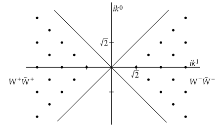
Figure 27: Extra physical states in the $(ik^{0},ik^{1})$ plane.

The corresponding operators are denoted $W_{s,n}^{\mp}(z)\tilde{W}_{s,n}^{\pm}(\bar{z})$. The lines $ik^{0}=\pm ik^{1}$ correspond to (imaginary) tachyon momenta. The $L_{0}$, $\tilde{L}_{0}$ conditions imply that the state $(s,n)$ is at level $s^{2}-n^{2}$.

Note also the conserved currents $\partial X^{0}$ and $\bar{\partial}X^{0}$, closely related to the operator $W_{1,0}^{+}\tilde{W}_{1,0}^{+}=\partial X^{0}\bar{\partial}X^{0}$. Actually, although these currents are separately conserved, their difference couples to the winding number in the $X^{0}$ direction. For the non-compact theory that we are concerned with this vanishes, so only one symmetry is nontrivial. At higher levels there are additional symmetries $A_{s,n}$, in one-to-one correspondence with the $W_{s,n}^{+}\tilde{W}_{s,n}^{+}$ (recall the result (4.1.2) that a spacetime symmetry corresponds to a BRST invariant operator of appropriate ghost number).

So the $D=2$ string theory does have a few graviton-dilaton states, and some interesting physics associated with them. In addition it has a large number of similar states at higher levels. The state $W_{1,0}^{-}\tilde{W}_{1,0}^{-}$ corresponds to a black hole background. It seems likely that the other $W_{s,n}^{-}\tilde{W}_{s,n}^{-}$ give rise to some infinite-parameter generalization of the black hole, but little is known about this; a formal argument for the existence of these solutions is given in ref. [167].

The tachyon state was obvious in the matrix model. So are the symmetries $A_{s,n}$—they are just the $v_{mn}$ introduced above for positive integer $m,n$ [168]-[171],

$$A_{s,n}\ \propto\ v_{s+n,s-n}.$$ (5.6.11)

This identification is consistent with the $(k^{0},k^{1})$ values. Also the linear term in the variation of the tachyon field is known to be the same, as is the algebra

$$\{v_{mn},v_{m^{\prime}n^{\prime}}\}=2(m^{\prime}n-n^{\prime}m)v_{m+m^{\prime}-1,n+n^{\prime}-1}.$$ (5.6.12)

This is the same as the $w_{\infty}$ commutator (1.7.13), with $4V^{i}_{m}\equiv v_{i+m+1,i-m+1}$. Only the range of the indices differs.

However, the remainder of the physical states are not so evident. The $W_{s,n}^{+}\tilde{W}_{s,n}^{+}$ do mix with the tachyons at the appropriate momenta and can be seen in matrix model correlators (reviewed in chapter 6 of ref. [135]). The $W_{s,n}^{-}\tilde{W}_{s,n}^{-}$ are, like the black hole, singular at large $X^{1}$ and do not appear in the matrix model in any simple way [137]. In the next section we will see that much of the physics of the discrete states is not contained within the matrix model by itself but also involves the mapping between the matrix model and the $D=2$ string theory.

5.7 Spacetime Gravity in the Matrix Model

The results of the previous section seem quite exciting. The $D=2$ string theory has black hole solutions, and we have in the matrix model an exact quantum solution to this theory. But things are not yet so rosy. First, we do not know how to describe the black hole in the matrix model language—what deformation of the matrix model corresponds to nonzero Schwarzchild mass $M$? Second, as we will discuss in section 5.8, we do not yet have the exact solution to the theory, only its perturbation expansion.

To begin to study this issue, we will first ask a much more basic question [172]. How, in the matrix model, do we see the gravitational interaction even between lumps of matter too diffuse to form a black hole? I will phrase this as an S-matrix question. Imagine sending two successive tachyon pulses in from the asymptotic region. The first pulse carries energy and momentum, so the second pulse must feel its gravitational field. There will then be some amplitude for the process shown in fig. 28a, in which part of the second pulse backscatters from the gravitational field of the first pulse.

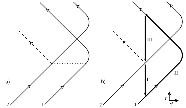
Figure 28: a) Successive pulses moving in the $t-q$ plane. Gravitational field (dotted) of pulse 1 will cause part of pulse 2 to backscatter, producing an outgoing wave (dashed) which precedes the main reflection from the wall. b) How the matrix model represents this process. The initial wavefunction renormalization (I) produces a tail on pulse 2 which overlaps pulse 1; the combined pulse reflects from the wall (II); and the final renormalization (III) produces the outgoing wave.

But this does not happen in the matrix model! The pulses consist of free fermions, which move independently in the inverted oscillator potential.

This would seem to be a contradiction, because I have set this up as an S-matrix question, and earlier I told you that the string and matrix model S-matrices agree. However, I also told you that there is a renormalization of the states, the leg pole factor (5.5.12), and this is in fact essential to seeing all of the physics. To see how the renormalization can have this effect, let us write it in coordinate space, in terms of the asymptotic incoming and outgoing tachyon fields:

$${\rm(I)}:\quad \overline{\cal S}_{+}(t-q)=\int_{-\infty}^{\infty}d\tau\,K(\tau){\cal S}_{+}(t-q-\tau)$$

$${\rm(III)}:\quad {\cal S}_{-}(t+q)=\int_{-\infty}^{\infty}d\tau\,K(\tau)\overline{\cal S}_{-}(t+q-\tau).$$ (5.7.1)

Here, a bar is again used to distinguish the matrix model quantity from the corresponding string quantity. The same kernel appears in both transformations,

$$K(\tau) = \int_{-\infty}^{\infty}\frac{d\omega}{2\pi}e^{i\omega\tau}\biggl{(}\frac{\pi}{2}\biggr{)}^{-i\omega/4}\frac{\Gamma(-i\omega)}{\Gamma(i\omega)}$$ (5.7.2)

$$= -\frac{z}{2}J_{1}(z),\qquad z=2(2/\pi)^{1/8}e^{\tau/2}.$$

This has asymptotic behaviors

$$K(\tau) \sim -\biggl{(}\frac{\pi}{2}\biggr{)}^{-1/4}e^{\tau},\qquad\tau\to-\infty$$ (5.7.3)

$$\sim \biggl{(}\frac{\pi}{2}\biggr{)}^{-1/16}\frac{e^{\tau/4}}{\sqrt{\pi}}\cos(z+\pi/4),\qquad\tau\to\infty.$$

To describe the scattering of an incoming ($+$) string tachyon pulse, one must (I) transform to the matrix model tachyon field via (5.7.1), (II) evolve the pulse as described in section 5.5, and (III) transform back. The transformation (5.7.1) is nonlocal, and it is the early-time behavior that is important. Although this falls exponentially, so does the gravitational effect (5.6.10) that we seek. As long as we use narrow enough pulses, gaussians, the exponential tail can be discerned [173], [172].

The string amplitude I-II-III does indeed display the gravitational scattering. This works as shown in fig. 28b. The transformation I on the incoming pulse 2 produces an early tail that overlaps pulse 1. These propagate together through the turning point and interact locally, and the transformation III produces the outgoing gravitationally scattered wave.

It will be useful for the later discussion to provide some details, but it is simpler for this to look at the slightly simpler process of $2\to 1$ bulk tachyon scattering. That is, as shown in fig. 29a, a pair of tachyons in one pulse can interact and scatter into one outgoing tachyon before reaching the wall.

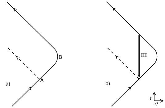
Figure 29: a) Two tachyons in an incoming pulse can backscatter into one (dashed line) at a given point A. In the matrix model all tachyons pass through the turning region B. b) The tail from transformation III produces the outgoing wave.

This occurs in the $D=2$ string theory, from direct calculation of the three string interaction, but it again does not occur in the matrix model because the fermions are free—they travel on hyperbolic phase space orbits and so reach the turning point of the potential. The leg pole transformation III is again responsible for the difference, as shown in fig. 29b; the tail on transformation I is not important in this case. Explicitly,

$$\lim_{t+q\to-\infty}{\cal S}_{-}(t+q) = -2^{1/4}\pi^{-1/4}e^{t}\int_{t}^{\infty}dt^{\prime}\,e^{-t^{\prime}}\overline{\cal S}_{-}(t^{\prime}+q)$$ (5.7.4)

$$= -2^{1/4}\pi^{-1/4}e^{t}\int_{-\infty}^{\infty}dt^{\prime}\,e^{-t^{\prime}}\overline{\cal S}_{-}(t^{\prime}+q)$$

$$= 2^{-3/4}\pi^{1/4}e^{t+q}v_{10}.$$

In the second line we have used the narrowness of the wavepacket to extend the range of integration, and in the third we have noted that the result is simply proportional to the conserved charge $v_{10}$. Now expressing this in terms of the incoming field gives

$$\lim_{t+q\to-\infty}{\cal S}_{-}(t+q) = 2^{-3/4}\pi^{1/4}e^{t+q}\int_{\infty}^{\infty}dt^{\prime}\,e^{-t^{\prime}+q}\Bigl{\{}(\partial_{t}\overline{\cal S}_{+}(t-q))^{2}+\overline{\mu}\partial_{t}\overline{\cal S}_{+}(t-q)/\sqrt{\pi}\Bigr{\}}$$ (5.7.5)

$$= 2^{-1/2}e^{t+q}\int_{\infty}^{\infty}dt^{\prime}\,e^{-t^{\prime}+q}({\cal S}_{+}(t^{\prime}-q))^{2}\ +\ O(\overline{\mu})\ .$$

In the second line we have carried out the renormalization (5.7.1), leading to a simple result after integration by parts. The $O(\overline{\mu})$ term is from $1\to 1$ scattering on the tachyon background.

The result (5.7.5) is the correct bulk scattering, as found from a string theory or effective field theory calculation [172]. Note in particular the exponential factor $e^{t-t^{\prime}+2q}$. At $t=t^{\prime}$, which is the point A in figure 29 where the incoming and outgoing rays meet, this is the trilinear string coupling $e^{2q}$.

In a sense, nothing here is new. In momentum space, we have simply found the graviton pole. It is well-known that this pole is not present in the matrix model amplitude but comes from the pole factors for the external legs [160]-[162], [174]-[176]. However, this coordinate space analysis makes a number of things much clearer, and dispels some confusions in the literature. One confusion is the frequent assertion that the leg pole factor is not relevant for physics in Minkowski space (real $\omega$), because it is a pure phase. We have seen that it is indeed essential for important Minkowski space physics—this is possible because the phase is a function of the momenta of the particles and so can be seen in interference. A second confusion is an identification of the string tachyon field with the macroscopic loop amplitude. This is not the same as the identification (5.7.1), and does not have the correct spacetime physics.

The coordinate space calculation also provides a physical interpretation for the discrete states in the cohomology. That is, they correspond to long-range forces not associated with propagating degrees of freedom. The imaginary values of the momenta for the discrete states correspond to exponential falloff of the forces in spacetime.

Let me emphasize that it is only the full string S-matrix I-II-III that is physical. That this factorizes into three separate parts, the first and third being linear in terms of the bosons, and the second being linear in terms of the fermions, is an accident of the $D=2$ kinematics and one should not give particular significance to the individual factors. Note also that the matrix model, in spite of its qualitative resemblance to the string spacetime, misrepresents the causal structure of the physics. The $2\to 1$ bulk process actually occurs at the point A in fig. 29a, before the pulse reaches the Liouville wall, but in the matrix model calculation the information in the incoming pulse always travels through the turning region B.

The scattering calculations here become more tedious at higher orders in the gravitational field and at higher levels. One would like to carry out the redefinition (5.7.1) directly in the Hamiltonian, converting the known matrix model Hamiltonian into a string Hamiltonian, with propagating tachyons plus long-ranged fields. The latter would presumably correspond to some gauge-fixing of string field theory. But one must add to the linear transformation (5.7.1) appropriate nonlinear terms to bring the Hamiltonian to this form, and this is does not seem to be simple.

5.8 Strong Nonlinearities

Now that we have detected weak field gravity, we would like to find the black hole solution. The first thing that comes to mind is to keep the field while omitting the source pulse 1, producing a source-free solution. But it is not evident how to do this, since the construction in fig. 28a depends in an essential way on the direct interaction between the two pulses. Various groups have proposed matrix model representations of the black hole background [177]. They take points of view different from my own, so it is hard to make a direct comparison. Several do emphasize the important point that the string theory is defined not by the matrix model alone (step II) but also by the mapping between the matrix model and string theory (steps I and III). But it is not clear that any of the proposal pass the test that they give the correct scattering in the weak field, weak coupling region studied in the previous section.

Since we have a complete description of the scattering of incoming pulses, we might try to make a black hole, by sending in a large enough pulse of matter. The perturbation (5.6.10) of the metric is $M/x^{4}$ in matrix model variables, so in order to form a black hole we need at least for this to be of order 1. Consider now a pulse on the Fermi sea, of width ${\mit\Delta}x$ and height ${\mit\Delta}p$. The total energy $M$ in the pulse is of order the number of fermions times the height above the Fermi level, or ${\mit\Delta}x\,{\mit\Delta}p\,{\mit\Delta}(p^{2})$. Now, ${\mit\Delta}x\,\raise 1.29167pt\hbox{$<$\kern-7.5pt\lower 4.30554pt\hbox{$\sim$}}\,x$ and ${\mit\Delta}(p^{2})\sim x{\mit\Delta}p$, so we need

$$({\mit\Delta}p)^{2}\ \raise 1.29167pt\hbox{$>$\kern-7.5pt\lower 4.30554pt\hbox{$\sim$}}\ x^{2}$$ (5.8.1)

to produce a gravitational effect of order 1. That is, the height of the pulse is comparable to the height of the whole sea. The tachyon self-interaction is then also of order 1, since the dispersion of the fermions in the pulse is large. In contrast to four dimensions, we cannot get into a situation where the gravitational interaction dominates. It has a long enough range to be detected, but not long enough to dominate. So we cannot be sure a priori that it is possible to make a black hole. We will have to be experimentalists, throwing in pulses with various properties and seeing if the result has any of the characteristic signatures of a black hole.

In fact, two interesting qualitative behaviors are found with large pulses [148]. The first is depicted in fig. 30a.

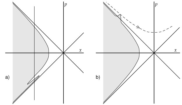
Figure 30: a) Outgoing pulse in which dispersion has produced a fold. At the indicated $x$, the Fermi sea has two filled bands separated by an empty band. b) Incoming pulse extending above the line $p=-x$. The fermions above the line pass over the potential barrier to $x=\infty$.

For a sufficiently tall or steep pulse dispersion will cause it to broaden past the vertical, producing an empty band in the Fermi sea and a double-valued Fermi surface. What does this correspond to in bosonic language? There is a one-to-one correspondence between single-valued Fermi surfaces and classical states of the bosonic field. By a classical state I mean one for which $\langle A^{2}\rangle=\langle A\rangle^{2}$ for any observable $A$, in the classical limit where the fermions become a continuous fluid. The double-valued surface does not, in this classical limit, correspond to a classical bosonic state. One can check this explicitly by calculating in such a sea the one-point and two-point functions of the boson modes $\overline{\alpha}(\omega)$, which are just the fermion currents. Even without calculation, a little thought will show that by moving fermions down into the empty band one can reduce the energy $\frac{1}{2}\int\{(\partial_{t}\overline{\cal S})^{2}+(\partial_{q}\overline{\cal S})^{2}\Bigr{\}}$ while keeping the expectation values of $\partial_{t}\overline{\cal S}$ and $\partial_{q}\overline{\cal S}$ fixed.

The double-valued surface is thus a bosonic state with a large amount of energy in addition to that in the classical field—that is, a large amount of radiation. There is a superficial resemblance here to formation of a black hole. In both cases, for incoming matter below a threshold (to form a horizon or a fold respectively), the incoming energy comes out again in the classical field. Above the threshold a non-negligible fraction of the incoming classical energy returns as radiation, Hawking radiation in the black hole and fold radiation in the matrix model. But here the resemblance ends. The fold radiation comes out too promptly, and it is too hot—typical energies of the quanta scale as $\hbar^{1/2}$ rather than $\hbar^{1}$.

It is not obvious how we would see the fold radiation if we had only the stringy, bosonic, description and not the fermionic one. In bosonic language the fold corresponds to an intersection of characteristics (null lines), which occurs because the velocity is a function of the tachyon field. In most situations where such a thing occurs, there are higher-derivative terms in the equation of motion which prevent double-valuedness and lead to formation of a shock wave. But that is not the case here—it is evident in the free fermionic language that pulse turns into a fold. So instead of a shock wave we get radiation, but I don’t know how to see this purely from the bosonic Hamiltonian. One rather different possibility is that the fold is a coordinate singularity, and that we need to unfold it by an appropriate coordinate transformation in phase space, but I do not know how to make sense of this.

The second interesting behavior is shown in fig. 30b. This is a pulse which extends above the line $p=-x$, so that some of the fermions pass over the barrier to the asymptotic region on the right. This certainly sounds like a black hole—we throw matter in and it doesn’t all come back out! But now we have to face a problem that we have deferred, the interpretation the other side of the potential barrier. In fact there is an infinite number of ways to define the matrix model, all of which give a unitary S-matrix and all of which have the same perturbation expansion [151] (and presumably the same as that of the string). One class of theories (type I in the terminology of ref. [151]) eliminates the second asymptotic region by modifying the potential. For example, a sharp infinite barrier, $V(x)=\infty$ for $x>A$, $A\geq 0$, leaves the perturbation theory with fixed numbers of incoming strings unaffected for any $A\geq 0$. So does any other modification such that $V(x)$ is $-\frac{1}{2}x^{2}$ for $x<0$ and rises to infinity as $x\to\infty$. All incoming fermions eventually return ot $x=-\infty$, so these are unitary quantum theories within the Hilbert space of incoming and outgoing fermions in the left asymptotic region (or the bosonized equivalent). The type II theory, on the other hand, leaves the potential unmodified and and fills both sides of the barrier to the same level. It is a unitary quantum theory but with two asymptotic Hilbert spaces. So there appears to be an infinite number of consistent nonperturbative definitions of the matrix model. Note that the ambiguity appears not only in the nonperturbative single-fermion tunneling amplitudes, but also in the large-field classical behavior. This is because a large incoming pulse can propagate into the strongly coupled region.

Our study of gravitational and bulk scattering now pays an unexpected bonus, for we have a new consistency condition which must be satisfied. Suppose we modify the potential by an infinite barrier at $x=A\geq 0$. A fermion reaching this barrier will jump suddenly from phase space point $(x,p)=(A,p)$ to $(A,-p)$. The quantities $v=(-x-p)e^{-t}$ and $w=(-x+p)e^{t}$ are no longer conserved, and neither will be the $v_{mn}$. Eq. (5.7.5) no longer holds and we get the wrong bulk amplitude. This violates causality—the bulk scattering occurs at the point A of fig. 29a, where string perturbation theory is valid and the incoming wave weak; the nonlinearity becomes large only later, at point B. A further acausality will be a nonconservation of gravitational mass in the process of fig. 28. This same argument applies to all modifications of type I, even if the potential rises more smoothly. Since $(-x-p)e^{-t}$ is negative for incoming fermions with $p>-x$ but positive on all outgoing trajectories on the left side, it can never be conserved. So all theories of type I are inconsistent. One can also see this another way—the $v_{mn}$ correspond to unbroken spacetime gauge symmetries and one would expect these to be conserved exactly.

The type II theory with unmodified potential conserves the $v_{mn}$, but it still gives rise to an inconsistent string theory, at least with the natural interpretation that the two asymptotic regions of the matrix model correspond to two asymptotic regions of spacetime. The point is that part of the conserved $v_{mn}$ passes over the barrier, so the first equality in eq. (5.7.5), relating $v_{10}$ to the outgoing field on the left only, no longer holds.

So I am saying that in spite of the substantial effort that went into matrix models no consistent nonperturbative construction of the $D=2$ string has yet been given. I think that this is much better than the previous situation of an infinite number of theories. The study of the bulk and gravitational scattering in coordinate space has not only dispels some confusions and clarifies the nature of the discrete states, but also provides a criterion for selecting among the possible nonperturbative definitions of the theory. The next step is to search for a solution to the consistency conditions, considering modification both of the matrix model itself and of the mapping between the matrix model and string theory. This is an important problem, bearing directly on the $e^{-C/g_{\rm c}}$ behavior, and I am optimistic that progress can be made.

5.9 Conclusion

In conclusion, let me say again that I think it likely that string theory will involve rich new dynamics that play an essential role in determining the ground state. Sometimes I feel that the tools I have described, such as the matrix model and the various high energy limits, are crude and unsophisticated. This is why I found the parallels with Wilson’s lecture so encouraging—both the feeling of clutching at straws, and the resemblance between his models and the matrix model. So perhaps the same method of attack that was so successful in quantum field theory will be useful again.

Acknowledgments

I would like to thank Mark Bowick, Shyamoli Chaudhuri, Jacques Distler, Jeff Harvey, Igor Klebanov, David Lowe, Makoto Natsuume, Phil Nelson, Andy Strominger, Lenny Susskind, and Lars Thorlacius for discussions of various points. I would also like to thank the students, organizers, and fellow lecturers of the school for their questions and comments, for an enjoyable experience, and for foosball lessons. This work was supported by NSF grants PHY-89-04035, PHY-91-16964, and PHY-94-07194.

References

- [1]
- [2] K. Wilson, Rev. Mod. Phys. 55, 583 (1983).
- [3] A. Giveon, M. Porrati, and E. Rabinovici, Phys. Rept. 244, 77 (1994).
- [4] P. Ginsparg, in Fields, Strings and Critical Phenomena, Les Houches Session XLIX, edited by E. Brezin and J. Zinn-Justin (Elsevier, 1989) 1.
- [5] J. L. Cardy, in Fields, Strings and Critical Phenomena, Les Houches Session XLIX, edited by E. Brezin and J. Zinn-Justin (Elsevier, 1989) 169.
- [6] D. Friedan, in Recent Advances in Field Theory and Statistical Mechanics, Les Houches Session XXXIX, edited by J.-B. Zuber and R. Stora (Elsevier, 1984) 839.
- [7] M. Peskin, in From the Planck Scale to the Weak Scale, TASI 1986, edited by H. Haber (World Scientific, 1987) 277.
- [8] T. Banks, in The Santa Fe TASI-87, edited by R. Slansky and G. West (World Scientific, 1988) 572.
- [9] S. B. Giddings, Phys.Rept. 170, 167 (1988).
- [10] E. D’Hoker, in Recent Directions in Particle Theory, TASI 1992, edited by J. Harvey and J. Polchinski (World Scientific, 1993) 1.
- [11] M. Green, J. Schwarz, and E. Witten, Superstring Theory, Vols. 1 and 2 (Cambridge, 1987).
- [12] A. M. Polyakov, Gauge Fields and Strings (Harwood, 1987).
- [13] D. Lust and S. Theisen, Lectures on String Theory (Springer-Verlag, 1989).
- [14] M. Kaku, Introduction to Superstrings (Springer-Verlag, 1988); Strings, Conformal Fields, and Topology (Springer-Verlag, 1991).
- [15] B. Hatfield, Quantum Field Theory of Point Particles and Strings (Addison-Wesley, 1992).
- [16] J. M. Drouffe and C. Itzykson, Statistical Field Theory, Vols. 1 and 2 (Cambridge, 1989).
- [17] C. Itzykson, H. Saleur, and J.-B. Zuber, eds., Conformal Invariance and Applications to Statistical Mechanics (World Scientific, 1988).
- [18] J. Polchinski, Joe’s Big Book of String (Cambridge, 1995?).
- [19] A. A. Belavin, A. M. Polyakov, and A. B. Zamolodchikov, Nucl. Phys. B241, 333 (1984).
- [20] D. Friedan, E. Martinec, and S. Shenker, Nucl. Phys. B271, 93 (1986).
- [21] S. Fubini, A. J. Hansen, and R. Jackiw, Phys. Rev. D7, 1732 (1973).
- [22] A. Chodos and C. B. Thorn, Nucl. Phys. B72, 509 (1974).
- [23] D. Friedan, Ann. Phys. 163, 318 (1985).
- [24] E. S. Fradkin and A. A. Tseytlin, Phys. Lett. 158B, 316 (1985); 160B, 69 (1985).
- [25] C.G. Callan, E.J. Martinec, M.J. Perry, and D. Friedan, Nucl. Phys. B262, 593 (1985).
- [26] E. Witten, Comm. Math. Phys. 92, 451 (1984).
- [27] V. Knizhnik and A. B. Zamolodchikov, Nucl. Phys. B247, 83 (1984).
- [28] D. Gepner and E. Witten, Nucl. Phys. B278, 493 (1986).
- [29] D. Friedan, Z. Qiu, and S. Shenker, Phys. Rev. Lett. 52, 1575 (1984).
- [30] V. S. Dotsenko and V. A. Fateev, Nucl. Phys. B240, 312 (1984); B251 691 (1985).
- [31] P. Goddard and D. Olive, Int. J. Mod. Phys. A1, 303 (1986).
- [32] P. Ramond, Phys. Rev. D3, 2415 (1971).
- [33] A. Neveu and J. H. Schwarz, Nucl. Phys. B31, 86 (1971).
- [34] M. Ademollo, et. al., Nucl. Phys. B111, 77 (1976); B114, 297 (1976); Phys. Lett. 62B, 105 (1976).
- [35] T. Eguchi and A. Taormina, Phys. Lett. B196, 75 (1987).
- [36] C. N. Pope. L. J. Romans, and X. Shen, in Proceedings of Strings ’90, edited by R. Arnowitt, et. al. (World Scientific, 1991) 287; X. Shen, Int. J. Mod. Phys. A7, 6953 (1992) hep-th/9202072.
- [37] P. Bouwknegt and K. Schoutens, Phys. Rept. B223, 183 (1993) hep-th/9210010.
- [38] C. Vafa, Phys. Lett. 199B, 195 (1987).
- [39] A. LeClair, M. E. Peskin, and C. R. Preitschopf, Nucl. Phys. B317, 411, 464 (1989).
- [40] J. Polchinski, Nucl. Phys. B307, 61 (1988).
- [41] H. Sonoda, Nucl. Phys. B311, 401,417 (1988).
- [42] J. L. Cardy, Nucl. Phys. B270, 186 (1986).
- [43] O. Alvarez, Nucl. Phys. B216, 125 (1983).
- [44] E. D’Hoker and D. H. Phong, Rev. Mod. Phys. 60, 917 (1988).
- [45] S. Weinberg, in General Relativity, An Einstein Centenary Survey, edited by S. W. Hawking and W. Israel (Cambridge, 1979) 790.
- [46] T. Yoneya, Nouvo Cim. Lett. 8, 951 (1973).
- [47] J. Scherk and J. H. Schwarz, Nucl. Phys. B81, 118 (1974).
- [48] P. Candelas, G. Horowitz, A. Strominger, and E. Witten, Nucl. B258, 46 (1985).
- [49] U. Amaldi, W. de Boer, and H. Furstenau, Phys. Lett. B260, 447 (1991).
- [50] A. M. Polyakov, Phys. Lett. B103, 207, 211 (1981).
- [51] J. Polchinski and A. Strominger, Phys. Rev. Lett. 67, 1681 (1991).
- [52] E. D’Hoker and S. B. Giddings, Nucl. Phys. B291, 90 (1987).
- [53] R. C. Brower, Phys. Rev. D6, 1655 (1972); P. Goddard and C. B. Thorn, Phys. Lett. 40B, 235 (1972).
- [54] D. M. Capper and M. J. Duff, Nuovo Cim. 23A, 173 (1974); Phys. Lett. 53A, 361 (1975).
- [55] L. Alvarez-Gaumé and E. Witten, Nucl. Phys. B234, 269 (1984).
- [56] T. Kugo and I. Ojima, Phys. Lett. 73B, 459 (1978); Suppl. Prog. Theor. Phys. 66, 1 (1979).
- [57] M. Henneaux and C. Teitelboim, Quantization of Gauge Systems (Princeton, 1992).
- [58] C. Becchi, A. Rouet, and R. Stora, Phys. Lett. 52B, 344 (1974); Ann. Phys. 98, 287 (1976).
- [59] M. Kato and K. Ogawa, Nucl. Phys. B212, 443 (1983).
- [60] M.D. Freeman and D.I. Olive, Phys. Lett. 175B, 151 (1986); C. B. Thorn, Nucl. Phys. B286, 61 (1987); I.B. Frenkel, H. Garland, and G.J. Zuckerman, Proc. Natl. Acad. Sci. 83, 8442 (1986).
- [61] D. J. Gross, J. A. Harvey, E. Martinec, and R. Rohm, Phys. Rev. Lett. 54, 502 (1985); Nucl. Phys. B256, 53 (1985); B267, 75 (1986).
- [62] M. B. Green and J. H. Schwarz, Nucl. Phys. B255, 93 (1985).
- [63] H. Ooguri and C. Vafa, Nucl. Phys. B361, 469 (1991).
- [64] S.-H. H. Tye, “Status of Fractional Superstrings,” presented at Strings ’93, Berkeley (1993) hep-th/9311021; K. R. Dienes, “Recent Developments in Fractional Superstrings,” presented at SUSY-93, Northeastern (1993) hep-th/9306156.
- [65] C. N. Pope, “W-Strings 93,” presented at Strings ’93, Berkeley (1993) hep-th/9309125.
- [66] J. L. Cardy and D. C. Lewellen, Phys. Lett. B259, 274 (1991); D. C. Lewellen, Nucl. Phys. B372, 654 (1992).
- [67] E. Martinec, Nucl. Phys. B281, 157 (1987).
- [68] B. Zwiebach, Nucl. Phys. B390, 33 (1993).
- [69] W. Fischler and L. Susskind, Phys. Lett. B171, 383 (1986); 173, 262 (1986).
- [70] P. Mansfield, Nucl. Phys. B283, 551 (1987).
- [71] J. H. Schwarz, Int. J. Mod. Phys. A4, 2653 (1989).
- [72] V. Kaplunovsky, Phys. Rev. Lett. 55, 299 (1985).
- [73] S. Jain, R. Shankar, and S. R. Wadia, Phys. Rev. D32, 2713 (1985).
- [74] A. B. Zamolodchikov, Sov. J. Nucl. Phys. 44; J. L. Cardy, in Phase Transitions and Critical Phenomena, Vol. 11, edited by C. Domb and J. L. Lebowitz (Academic, 1986).
- [75] T. Banks, L. Dixon, D. Friedan, and E. Martinec, Nucl. Phys. B299, 613 (1988).
- [76] C. L. Kane, M. P. A. Fisher, and J. Polchinski, Phys. Rev. Lett. 72, 4129 (1994) cond-mat/9402108.
- [77] K. Kikkawa and M. Yamanaka, Phys. Lett. B149, 357 (1984); N. Sakai and I. Senda, Prog. Theor. Phys. 75, 692 (1986).
- [78] A. A. Tseytlin, presented at the 2nd Journée Cosmologie, Observatoire de Paris (1994) hep-th/9407099.
- [79] T. Buscher, Phys. Lett. B159, 127 (1985); B194, 59 (1987); B201, 466 (1988).
- [80] M. Dine, P. Huet, and N. Seiberg, Nucl. Phys. B322, 301 (1989).
- [81] S. Giddings, J. Polchinski, and A. Strominger, Phys. Rev. D48, 5784 (1993).
- [82] R. Dijkgraaf, E. Verlinde, and H. Verlinde, in Perspectives in String Theory, edited by P. Di Vecchia and J. L. Petersen (World Scientific, 1988); A. Shapere and F. Wilczek, Nucl. Phys. B320, 669 (1989).
- [83] S.-T. Yau, ed., Essays on Mirror Manifolds, (International Press, 1992).
- [84] A. Giveon and E. Witten, Phys. Lett. B332, 44 (1994) hep-th/9404184.
- [85] J. Dai, R. Leigh, and J. Polchinski, Mod. Phys. Lett. A4, 2073 (1989).
- [86] R. Leigh, Mod. Phys. Lett. A4, 2767 (1989).
- [87] N. Berkovits and C. Vafa, Mod. Phys. Lett. A9, 653 (1994) hep-th/9310170.
- [88] F. Bastianelli, N. Ohta, and J. L. Petersen, Phys. Rev. Lett. 73, 1199 (1994) hep-th/9403150.
- [89] N. Berkovits, M. Freeman, and P. West, Phys. Lett. B325, 63 (1994) hep-th/9312013.
- [90] H. Kunitomo, M. Sakaguchi, and A. Tokura, “A Universal String Theory,” Osaka preprint OU-HET-187 (1994) hep-th/9403086; “A Heirachy of Super Strings,” Osaka preprint OU-HET-199 (1994) hep-th/9408007.
- [91] H. Kunitomo, “On the Nonlinear Realization of the Superconformal Symmetry,” Osaka preprint OU-HET-196 (1994) hep-th/9407052.
- [92] A. Font, L. Ibanez, D. Lüst and F. Quevedo, Phys. Lett. B249, 35 (1990).
- [93] A. Sen, Int. J. Mod. Phys. A9, 3707 (1994) hep-th/9402002.
- [94] P. A. M. Dirac, Proc. R. Soc. A133, 60 (1931).
- [95] E. Witten, Phys. Lett. B86, 286 (1979).
- [96] C. Montonen and D. Olive, Phys. Lett. B72, 117 (1977).
- [97] P. Goddard, J. Nuyts, and D. Olive, Nucl. Phys. B125, 1 (1977).
- [98] E. Witten and D. Olive, Phys. Lett. B78, 97 (1978).
- [99] H. Osborn, Phys. Lett. B83, 321 (1979).
- [100] A. Sen, Phys. Lett. B329, 217 (1994) hep-th/9402032.
- [101] N. Seiberg and E. Witten, Nucl. Phys. B426, 19 (1994) hep-th/9407087.
- [102] “Monopoles, Duality, and Chiral Symmetry Breaking in Supersymmetric QCD,” N. Seiberg and E. Witten, preprint RU-94-60 (1994) hep-th/9408099.
- [103] “A Strong Coupling Test of -Duality,” C. Vafa and E. Witten, preprint HUTP-94-A017 (1994) hep-th/9408074.
- [104] M. J. Duff, Class. Quantum. Grav. 5, 189 (1988); A. Strominger, Nucl. Phys. B343, 167 (1990).
- [105] W. Siegel, Phys. Lett. 151B, 391, 396 (1984).
- [106] E. Witten, Nucl. Phys. B268, 253 (1986).
- [107] C. Thorn, Phys. Rept. 175, 1 (1989).
- [108] W. Siegel, Introduction to String Field Theory (World Scientific, 1988).
- [109] R. Brustein and S. P. de Alwis, Nucl. Phys. B352, 451 (1991); R. Brustein and K. Roland, Nucl. Phys. B372, 201 (1992).
- [110] S. B. Giddings, E. Martinec, and E. Witten, Phys. Lett. B176, 362 (1986).
- [111] W. Siegel, Phys. Rev. D49, 4144 (1994) hep-th/9312117.
- [112] A. Strominger, Nucl. Phys. B294, 93 (1987).
- [113] J. Polchinski, Comm. Math. Phys. 104, 37 (1986).
- [114] J.-C. Le Guillou and J. Zinn-Justin, eds., Large-Order Behavior of Perturbation Theory, Current Physics Sources and Comments, Vol. 7 (North-Holland, 1990).
- [115] D. Gross and V. Periwal, Phys. Rev. Lett. 60, 2105 (1988).
- [116] S. Shenker, in Random Surfaces and Quantum Gravity, edited by O. Alvarez, E. Marinari, and P. Windey (Plenum, 1991).
- [117] J. Polchinski, “Combinatorics of Boundaries in String Theory,” preprint NSF-ITP-94-52 (1994) hep-th/9407031.
- [118] A. D’Adda, M. Lüscher and P. Di Vecchia, Nucl. Phys. B146, 63 (1978); B152, 125 (1979).
- [119] E. Fradkin, Field Theories of Condensed Matter Systems (Addison-Wesley, 1991).
- [120] S. Weinberg and E. Witten, Phys. Lett. 96B, 59 (1980).
- [121] J. J. Atick and E. Witten, Nucl. Phys. B310, 291 (1988).
- [122] C. B. Thorn, in Sakharov Memorial Lectures in Physics, proceedings of the First International Sakharov Conference on Physics, Moscow, edited by L.V. Keldysh and V. Ya. Fainberg (Nova Science, 1991) 447; hep-th/9405069.
- [123] L. Susskind, “The World as a Hologram,” preprint SU-ITP-94-33 (1994) hep-th/9409089.
- [124] D. J. Gross and P. F. Mende, Phys. Lett. 197B, 129 (1987); Nucl. Phys. B303, 407 (1988).
- [125] P. F. Mende and H. Ooguri, Nucl. Phys. B339, 641 (1990).
- [126] D. J. Gross, Phys. Rev. Lett. 60, 1229 (1988).
- [127] D. Amati, M. Ciafaloni, and G. Veneziano, Phys. Lett. B216, 41 (1989).
- [128] L. Susskind, Phys. Rev. Lett. 71, 2367 (1993) hep-th/9307168.
- [129] A. Mezhlumian, A. Peet, and L. Thorlacius, Phys. Rev. D50, 2725 (1994) hep-th/9402125.
- [130] P. Salomonson and B.-S. Skagerstam, Nucl. Phys. B268, 349 (1986).
- [131] D. Mitchell and N. Turok, Phys. Rev. Lett. 58, 1577 (1987); Nucl. Phys. B294, 1138 (1987).
- [132] R. Brandenberger and C. Vafa, Nucl. Phys. B316, 391 (1989).
- [133] D. A. Lowe and L. Thorlacius, “Hot String Soup,” preprint NSF-ITP-94-83, UCSBTH-94-30 (1994) hep-th/9408134.
- [134] P. Ginsparg and G. Moore, in Recent Directions in Particle Theory, Proceedings of the 1992 TASI, edited by J. Harvey and J. Polchinski (World Scientific 1993) hep-th/9304011.
- [135] I. Klebanov, in String Theory and Quantum Gravity, Proceedings of the Trieste School 1991, edited by J. Harvey et. al. (World Scientific, 1992) hep-th/9108019.
- [136] R. C. Myers, Phys. Lett. B199, 371 (1988); I. Antoniades, C. Bachas, J. Ellis, and D. Nanopoulos, Phys. Lett. B211, 393 (1988).
- [137] N. Seiberg, Prog. Theor. Phys. Suppl. 102, 319 (1990).
- [138] J. Polchinski, in Proceedings of Strings ’90, edited by R. Arnowitt, et. al. (World Scientific, 1991) 62.
- [139] J. Polchinski, Nucl. Phys. B346, 253 (1990).
- [140] E. Brézin, C. Itzykson, G. Parisi, and J.-B. Zuber, Comm. Math. Phys. 59, 35 (1978).
- [141] E. Brézin, C. Itzykson, and J.-B. Zuber, Adv. App. Math. 1, 109 (1980).
- [142] V. A. Kazakov and A. A. Migdal, Nucl. Phys. B311, 171 (1988).
- [143] E. Brézin, V. A. Kazakov, and A. B. Zamolodchikov, Nucl. Phys. B333 (1990) 673; P. Ginsparg and J. Zinn-Justin, Phys. Lett. B240 (1990) 333; G. Parisi, Phys. Lett. B238, 209 (1990); D. J. Gross and N. Miljković, Phys. Lett. B238, 217 (1990).
- [144] D. Gross and A. Migdal, Phys. Rev. Lett. 64, 127 (1990); M. Douglas and S. Shenker, Nucl. Phys. B335, 635 (1990); E. Brezin and V. Kazakov, Phys. Lett. 236, 144 (1990).
- [145] T. L. Curtright and C. B. Thorn, Phys. Rev. Lett. 48, 1309 (1982); V. Knizhnik, A. Polyakov, and A. Zamolodchikov, Mod. Phys. Lett. A3, 819 (1988); F. David, Mod. Phys. Lett. A3, 1651 (1988); J. Distler and H. Kawai, Nucl. Phys. B321 (1989) 509.
- [146] E. D’Hoker, in Particle Physics, VI J. A. Swieca Summer School, edited by O. Eboli, M. Gomes, and A. Santoro, (World Scientific, 1992) 282.
- [147] S. R. Das and A. Jevicki, Mod. Phys. Lett. A5, 1639 (1990).
- [148] J. Polchinski, Nucl. Phys. B362, 125 (1991).
- [149] A. M. Sengupta and S. R. Wadia, Int. J. Mod. Phys. A6, 1961 (1991).
- [150] I. Klebanov, private communication.
- [151] G. Moore, M. R. Plesser, and S. Ramgoolam, Nucl. Phys. B377, 143 (1992) hep-th/9111035.
- [152] E. Smith, Nucl. Phys. B382, 229 (1992) hep-th/9201049; Phys. Lett. B305, 344 (1993) hep-th/9208039; R. E. Rudd, Ph. D. Thesis, Princeton (1992) unpublished.
- [153] N. Ishibashi and H. Kawai, Phys. Lett. B314, 190 (1993) hep-th/9307045; M. Ikehara, N. Ishibashi, H. Kawai, T. Mogami, R. Nakayama, and N. Sasakura, “String Field Theory in the Temporal Gauge,” preprint KEK-TH-402 (1994) hep-th/9406207.
- [154] Z. Yang (Texas U.), Phys. Lett. B257, 40 (1991); J. A. Minahan, Int. J. Mod. Phys. A8, 3599 (1993) hep-th/9204013.
- [155] V. A. Kazakov and I. K. Kostov, Nucl. Phys. B386, 520 (1992) hep-th/9205059; I. K. Kostov (Saclay), “Field Theory of Open and Closed Strings with Discrete Target Space,” preprint SACLAY-SPHT-94-097 (1994) hep-th/9410164.
- [156] E. Marinari and G. Parisi, Phys. Lett. B240 (1990) 375.
- [157] S. Chaudhuri and J. Polchinski, “Critical Behavior of the Marinari-Parisi Model,” preprint NSF-ITP-94-53 (1994) hep-th/9408005.
- [158] G. Moore and R. Plesser, Phys. Rev. D46, 1730 (1992) hep-th/9203060.
- [159] J. Polchinski, “On the Nonperturbative Consistency of String Theory,” preprint NSF-ITP-94-96 (1994) hep-th/9409168.
- [160] P. Di Francesco and D. Kutasov, Phys. Lett. B261, 385 (1991); Nucl. Phys. B375, 119 (1992).
- [161] A. M. Polyakov, Mod. Phys. Lett. A6, 635 (1991); in Two Dimensional Quantum Gravity and Random Surfaces, 8th Jerusalem Winter School for Theoretical Physics, Jerusalem, edited by D.J. Gross, T. Piran and S. Weinberg (1990-91) 175.
- [162] D. J. Gross and I. R. Klebanov, Nucl. Phys. B359, 3 (1991).
- [163] E. Witten, Phys. Rev. D44 (1991) 314.
- [164] G. Mandal, A Sengupta, and S. Wadia, Mod. Phys. Lett. A6 (1991) 1685.
- [165] R. Dijkgraaf, E. Verlinde, and H. Verlinde, Nucl. Phys. B371, 269 (1992).
- [166] E. Witten, Nucl. Phys. B373, 187 (1992) hep-th/9108004; E. Witten and B. Zwiebach, Nucl. Phys. B377, 55 (1992) hep-th/9201056.
- [167] S. Mukherji, S. Mukhi, and A. Sen, Phys. Lett. B275, 39 (1992).
- [168] J. Avan and A. Jevicki, Phys. Lett. B266, 35 (1991).
- [169] G. Moore and N. Seiberg, Int. J. Mod. Phys. A7, 2601 (1992).
- [170] S. R. Das, A. Dhar, G. Mandal, and S. R. Wadia, Int. J. Mod. Phys. A7, 5165 (1992) hep-th/9110021.
- [171] D. Minic, J. Polchinski, and Z. Yang, Nucl. Phys. B369, 324 (1992).
- [172] M. Natsuume and J. Polchinski, Nucl. Phys. B424, 137 (1994) hep-th/9402156.
- [173] M. Natsuume, “Zero Mode Divergence Problem in String Theory,” preprint NSF-ITP-93-157 (1993) hep-th/9401013.
- [174] N. Sakai and Y. Tanii, Prog. Theor. Phys. Suppl. 110, 117 (1992) hep-th/9111049; Phys. Lett. B276, 41 (1992) hep-th/9108027.
- [175] D. Minic and Z. Yang, Phys. Lett. B274, 27 (1992) hep-th/9109012.
- [176] D. Lowe, Mod. Phys. Lett. A7, 2647 (1992) hep-th/9204084.
- [177] A. Dhar, G. Mandal, and S. R. Wadia, Mod. Phys. Lett. A7, 3703 (1992) hep-th/9210120; ; A8 1701, (1993) hep-th/9304072; S. R. Das, Mod. Phys. Lett. A8, 69 (1993) hep-th/9210107; A8, 1331 (1993) hep-th/9303116; A. Jevicki and T. Yoneya, Nucl. Phys. B411, 64 (1994) hep-th/9305109.