NSF-ITP-94-109
hep-th/9411020
Black Hole Evolution

Abstract

Black hole formation and evaporation is studied in the semiclassical approximation in simple 1+1-dimensional models, with emphasis on issues related to Hawking’s information paradox. Exact semiclassical solutions are described and questions of boundary conditions and vacuum stability are discussed.

The validity of the semiclassical approximation has been called into question in the context of the information puzzle. A different approach, where black hole evolution is assumed to be unitary, is described. It requires unusual causal properties and kinematic behavior of matter that may be realized in string theory.

Based on lectures given at the 1994 Trieste Spring School on String Theory, Gauge Theory, and Quantum Gravity.

1 Introduction

Hawking’s discovery of black hole evaporation [1] has presented us with a unique window on the interplay between gravity and quantum physics. The puzzles of black hole evolution highlight the incompatibility between the world view offered by Einstein’s general relativity and that of quantum theories. The so called black hole information paradox, first formulated by Hawking [2], is a good example.

Consider an initial state of diffuse matter undergoing gravitational collapse and assume that the system starts out in a pure quantum mechanical state. According to classical gravitational theory, once the collapsing matter approaches its own Schwarzschild radius the external world only retains information about the total energy and conserved gauge charges carried by the infalling matter. This follows from a series of uniqueness theorems for solutions of general relativity coupled to various types of matter fields [3], which are collectively referred to as “no-hair” theorems. Observers outside the black hole no longer have access to all the degrees of freedom of the system and cannot describe it by a pure state. There is nothing wrong with that, as long as we consider only classical solutions of the gravitational field, for we can postulate that the missing information is hidden in the black hole and that the quantum state of the whole system remains pure even if outside observers have to resort to a density matrix description.

But now the black hole evaporates and according to Hawking’s semiclassical calculation the emitted radiation is thermal. Let us for the moment assume that the evaporation leaves no remnant behind so that the final state consists only of outgoing Hawking radiation, which, being thermal, is described by a mixed quantum state. It then appears that this process of black hole formation and subsequent evaporation evolves a pure state into a mixed one in direct violation of the basic rule that every quantum mechanical system should have a unitary evolution.

Hawking suggested to take this at face value and claimed that this is an example of an added fundamental uncertainty introduced into quantum physics, over and above the usual Heisenberg uncertainty, when gravitational effects are taken into account [4]. He further proposed a modified set of axioms for quantum field theory, which would allow pure states to evolve into mixed states. In his formalism the unitary $S$-matrix of quantum field theory, which maps an initial quantum state to a final state, is to be replaced by a superscattering operator $, which maps an initial density matrix to a final density matrix. In ordinary quantum field theory the superscattering operator factorizes, $ $=S\bar{S}$, but when gravity enters the game this is no longer true, due to black hole formation or even virtual processes involving gravitational fluctuations. Hawking’s proposal was criticized by a number of authors [5, 6, 7], and recently Strominger [8] pointed out that Hawking’s original proposal violates the superposition principle.

An alternative viewpoint, first suggested by Page [9] and strongly advocated by ’t Hooft [10], is that the Hawking radiation is not really exactly thermal but in fact carries all the information about the initial state of the infalling matter. This information is encoded in subtle correlations between quanta emitted at different times during the evaporation process, and detecting it would require a large number of statistical observations to be made on an ensemble of identically prepared states. This viewpoint is a conservative one from the point of view of quantum theory, since it insists on the existence of a unitary $S$-matrix, but it appears to require radical assumptions about the kinematic behavior of matter at high energies [10, 11]. Sections 5-7 of these lecture notes will be concerned with some recent work where this viewpoint is adopted.

A third possibility, advocated by Aharonov, Casher, and Nussinov [12], is that a black hole does not completely evaporate and the information is carried off by a Planck scale remnant. There would need to be a distinct remnant for each possible initial state, so the density of these remnant states at the Planck energy must be virtually infinite. This leads to thorny phenomenological problems if the remnants behave at all like local objects and their effects on low-energy physics can be described by an effective field theory. Even if individual remnant states couple extremely weakly to processes such as $e^{+}$-$e^{-}$ scattering at a colliding beam facility, the infinite density of states would cause them to be the dominant channel. One would also expect a divergent pair production rate of remnants in weak background fields and thermal sums would be rendered ill defined by their contribution. None of these effects are observed so either black holes do not leave behind information carrying remnants or those remnants are described by unconventional laws of physics at low energies. Considerable effort has gone into developing a picture of remnant dynamics [13] where the above pathologies are to be avoided. This work was described in detail in the lectures of Banks at this Spring School.

Recently Polchinski and Strominger [14] have argued that Hawking’s superscattering approach can be successfully reformulated as a unitary theory, with long-lived remnants, in the context of a third quantized theory of gravity. This interesting proposal will not be discussed here.

The information puzzle is an important theoretical problem because the resolution of the paradox may require a revision of some fundamental physical laws. Since we are unlikely to obtain laboratory data on quantum effects in gravity any time soon, confronting our theories with physical paradoxes of this type is one of the most promising lines of inquiry in this area of theoretical physics.

These lecture notes consist of two parts, each of which is to a large extent self-contained. The first part is a review of black hole physics in two spacetime dimensions with a view towards the information problem. In Section 2 we introduce a two-dimensional model, proposed by Callan, Giddings, Harvey, and Strominger (CGHS) [15] for black hole physics, and study its classical solutions. In Section 3 we consider the quantum theory of matter fields in a classical background black hole geometry and exhibit the two-dimensional analog of the Hawking effect. We give simple arguments for the thermal character of the Hawking radiation and then show how its back-reaction on the geometry can be accounted for via a set of semiclassical corrections to the equations of motion. In Section 4 we adopt a more systematic approach to the quantization of these two-dimensional models. We consider conformally invariant effective theories which reduce to the CGHS model in the classical limit. We address a number of issues which come up in the study of these models, such as the rate of Hawking evaporation, boundary conditions in the strong coupling region, and vacuum stability.

The second part of the lecture notes, beginning with Section 5, describes a different approach to black hole evolution where it is assumed from the outset that the information is returned in the Hawking radiation. In Section 5 we put forward a phenomenological framework for black hole physics which is consistent with a unitary evolution of quantum states. It is argued that any model where information is returned encoded in the Hawking radiation will have to incorporate a principle of black hole complementarity, which allows for the different viewpoints of an observer, who enters a black hole in free fall, and of an observer who remains outside at all times. In Section 6 we consider some gedanken experiments designed to test the validity of the complementarity hypothesis and find that their detailed analysis requires knowledge of Planck scale effects. This indicates that the information paradox is not well posed in terms of low-energy physics alone. In Section 7 we describe some recent work which suggests that string theory implements black hole complementarity in a natural way. The key observation in this context is that string matter exhibits very different kinematic behavior at high energies than matter formed out of weakly interacting pointlike particles.

2 Classical Dilaton Gravity in 1+1 Dimensions

When faced with a difficult problem it is often useful to look for a simpler toy system, in which an analogous problem can be posed and studied and, in the best of all worlds, solved. In the case of the black hole information puzzle such a simplified context is provided by certain two-dimensional models of gravity which have been actively studied (but unfortunately not fully solved) in recent years. These theories are far from being realistic models of real gravity since crucial ingredients of the four-dimensional physics, such as propagating gravitons, are missing. The simple toy theories do, however, have black hole geometries as classical solutions. When one considers the quantum theory of matter fields in such spacetimes one finds Hawking radiation and, at the semiclassical level, its back-reaction on the geometry leads to an information paradox, which is entirely analogous to the one posed by Hawking. The fate of quantum information is an important question of principle and it seems worth looking for an answer in this simplified context even if it is not at all guaranteed to reflect accurately on the situation in a more realistic setting.

A large number of papers has been written on various aspects of two-dimensional black hole physics in recent years. For reviews see e.g. [16, 17].

2.1 The CGHS Model

The CGHS model [15] of two-dimensional dilaton gravity, coupled to scalar matter fields, was proposed a few years ago as a particularly convenient toy model for black hole physics. The classical dynamics is governed by the action

$$S_{0}=\frac{1}{2\pi}\int d^{2}y\sqrt{-g}\Bigl{[}e^{-2\phi}(R+4(\nabla\phi)^{2}+4\lambda^{2})$$ (1)

$$-\frac{1}{2}\sum^{N}_{i=1}(\nabla f_{i})^{2}\Bigr{]}\,,$$

which can be viewed as an effective action for radial modes of near-extremal magnetically charged black holes in four-dimensional dilaton gravity [15, 18, 19]. We will primarily be interested in this theory on its own merits as a two-dimensional model of gravity coupled to matter, but the higher-dimensional interpretation is helpful in developing an intuitive picture of some aspects of the physics.

The action (1) inherits a length scale $\lambda^{-1}$ from the four-dimensional geometry, which is set by the magnetic charge of the extremal black hole, $\lambda^{-1}=2Q$. We shall use units in which $\lambda=1$ throughout. In the region of the four-dimensional geometry where the two-dimensional effective description applies, the physical radius of the local transverse two-sphere is given by the dilaton field, $r(x^{0},x^{1})=e^{-\phi(x^{0},x^{1})}$.

The classical equations of motion are

$$\!\!\begin{array}[]{l}\nabla^{2}f_{i}=0\,,\\ {}\\ {1\over 4}R+\nabla^{2}\phi-(\nabla\phi)^{2}+1=0\,,\\ {}\\ \nabla_{\mu}\nabla_{\nu}\phi+g_{\mu\nu}((\nabla\phi)^{2}-\nabla^{2}\phi-1)={e^{2\phi}\over 2}T^{f}_{\mu\nu}\,,\end{array}$$ (2)

where $T^{f}_{\mu\nu}$ is the matter energy-momentum tensor,

$$T^{f}_{\mu\nu}={1\over 2}\sum_{i=1}^{N}\bigl{[}\nabla_{\mu}f_{i}\nabla_{\nu}f_{i}-{1\over 2}(\nabla f_{i})^{2}\bigr{]}\,.$$ (3)

It is convenient to work in conformal gauge and choose lightcone coordinates $y^{\pm}=y^{0}\pm y^{1}$, for which the line element is

$$ds^{2}=-{1\over 2}e^{2\rho}dy^{+}dy^{-}\,.$$ (4)

The fields in the theory are then $f_{i}$, $\phi$, and the conformal factor $\rho$. The classical equations of motion of these fields can be arranged to read

$$\!\!\begin{array}[]{l}\partial_{+}\partial_{-}f_{i}=0\,,\\ {}\\ \partial_{+}\partial_{-}(e^{-2\phi})=-e^{2(\rho-\phi)}\,,\\ {}\\ \partial_{+}\partial_{-}(\rho-\phi)=0\,.\end{array}$$ (5)

In addition, one must impose as constraints the equations of motion corresponding to the components of the metric that have been set to zero by this choice of gauge,

$$\!\!\begin{array}[]{l}e^{-2\phi}(2\partial_{+}^{2}\phi-4\partial_{+}\rho\partial_{+}\phi)=T^{f}_{++}\,,\\ {}\\ e^{-2\phi}(2\partial_{-}^{2}\phi-4\partial_{-}\rho\partial_{-}\phi)=T^{f}_{--}\,.\end{array}$$ (6)

The non-vanishing components of the matter energy-momentum tensor are given by $T^{f}_{\pm\pm}={1\over 2}\sum_{i=1}^{N}(\partial_{\pm}f_{i})^{2}$, and the conservation of matter energy-momentum takes the form $\partial_{-}T^{f}_{++}=0=\partial_{+}T^{f}_{--}$ in the classical theory. The left moving energy flux $T^{f}_{++}$ is only a function of the left moving lightcone coordinate $y^{+}$ and the right moving flux $T^{f}_{--}$ only depends on $y^{-}$.

One of the conformal gauge equations (5) is $\partial_{+}\partial_{-}(\rho-\phi)=0$, which has the general solution $\rho=\phi+f_{+}(y^{+})+f_{-}(y^{-})$. The arbitrary functions $f_{+}$ and $f_{-}$ can be eliminated by a conformal reparametrization to coordinates $(x^{+},x^{-})$ such that $dx^{+}/dy^{+}=e^{2f_{+}}$ and $dx^{-}/dy^{-}=e^{2f_{-}}$. This special coordinate system is referred to as Kruskal coordinates for reasons which will become apparent a little later on.

Since $\rho=\phi$ in Kruskal gauge the equations of motion and constraints reduce to

$$\!\!\begin{array}[]{l}\partial_{+}\partial_{-}e^{-2\phi}=-1\,,\\ {}\\ \partial_{\pm}^{2}e^{-2\phi(x^{+},x^{-})}=-T^{f}_{\pm\pm}(x^{\pm})\,,\end{array}$$ (7)

Let us first consider solutions with vanishing flux of matter energy, $T^{f}_{\pm\pm}=0$. The simplest one is the so called linear dilaton vacuum,

$$\!\!\begin{array}[]{l}f_{i}=0\,,\\ {}\\ e^{-2\phi}=e^{-2\rho}=-x^{+}x^{-}\,.\end{array}$$ (8)

This geometry has vanishing curvature everywhere. It derives its name from its expression in the coordinate system $(\sigma^{+},\sigma^{-})$ defined by the transformation $x^{\pm}=\pm e^{\pm\sigma^{\pm}}$, where the metric is manifestly flat, $\rho=0$, and the dilaton is linear in the spatial coordinate, $\phi=-(\sigma^{+}-\sigma^{-})/2=-\sigma^{1}$.

Due to the factor of $e^{-2\phi}$ in front of the dilaton-gravity terms in the action (1) the value of the dilaton field controls the strength of gravitational quantum corrections in the theory. In the linear dilaton vacuum the coupling varies with spatial position, ranging monotonically from infinite strength in the limit $\sigma^{1}\rightarrow-\infty$ to zero as $\sigma^{1}\rightarrow+\infty$. From the 3+1-dimensional viewpoint $\sigma^{1}$ is a radial coordinate and the weakly coupled region corresponds to asymptotic transverse two-spheres of large radius, while the strong coupling at $\sigma^{1}\rightarrow-\infty$ reflects the fact that the transverse area is going to zero and short-distance effects are becoming important. In general one expects significant quantum corrections to the spacetime metric where the coupling is strong and in some models the internal asymptotic region is replaced, as we shall see later on, by a timelike boundary which can be interpreted as the origin of radial coordinates.

2.2 Eternal Black Holes

In classical general relativity a black hole is defined as a region of spacetime which is not in the causal past of future null infinity ${\cal I}^{+}$ [3]. This means that no timelike observer can escape from a black hole since even null radiation is trapped. The boundary of the black hole is a null surface, called the global event horizon. Local observers cannot determine from local initial data whether they are inside a black hole. In order to locate the global event horizon one must have knowledge of future evolution of the entire spacetime manifold and be able to find the causal past of ${\cal I}^{+}$.

The linear dilaton vacuum (8) is a special case of a one-parameter family of static solutions:

$$\!\!\begin{array}[]{l}f_{i}=0\,,\\ {}\\ e^{-2\phi}=e^{-2\rho}=M_{0}-x^{+}x^{-}\,.\end{array}$$ (9)

The scalar curvature of these geometries is

$$R=8e^{-2\rho}\partial_{+}\partial_{-}\rho={4M_{0}\over M_{0}-x^{+}x^{-}}\,.$$ (10)

For $M_{0}\neq 0$ there are two curvature singularities which asymptotically approach the null curves $x^{\pm}=0$. The gravitational coupling strength diverges at these singularities.

If $M_{0}<0$ the singularities are timelike and the future of any Cauchy surface contains a naked singularity, i.e. one which is visible from ${\cal I}^{+}$.

For $M_{0}>0$ the curvature singularities are spacelike. One of them is a white hole singularity, which is not in the causal future of any event, and the other one is a black hole singularity encompassed by a global event horizon, which consists of two null line segments, $\{x^{+}{=}0,\ x^{-}{>}0\}$ and $\{x^{-}{=}0,\ x^{+}{>}0\}$. The parameter $M_{0}$ is proportional to the canonical ADM mass of the black hole [21].

The Penrose diagram in Figure 1 is obtained by making the conformal reparametrization $q^{\pm}=\arctan{(x^{\pm}/\sqrt{M_{0}})}$. It shows that the global causal structure of a static 1+1-dimensional black hole is completely analogous to that of the maximally extended Schwarzschild solution in 3+1 dimensions[3].

Figure 1: Penrose diagram for static black hole.

The value of the dilaton field at the event horizon is $e^{2\phi_{H}}=1/M_{0}$, so the strength of the gravitational coupling at the event horizon can be made arbitrarily weak by considering a black hole of large mass. The scalar curvature at the event horizon is $R_{H}=4$, independent of the black hole mass.

In the asymptotic region, where $x^{+}x^{-}\rightarrow-\infty$, the curvature goes to zero. The coordinate transformation $\sigma^{\pm}=\pm\log{x^{\pm}}$, puts the metric into a manifestly asymptotically flat form:

$$e^{2\rho}=(1+M_{0}\,e^{-2\sigma^{1}})^{-1}\,.$$ (11)

The $\sigma$-coordinate system only covers the region of spacetime which is outside the global event horizon and is analogous to the tortoise coordinates used to describe the Schwarzschild solution outside a black hole in 3+1 dimensions. The maximal analytic extension of the Schwarzschild solution is obtained by transforming to Kruskal coordinates and the same is achieved in the 1+1-dimensional case by going to the $(x^{+},x^{-})$ coordinate system, which is named accordingly.

We close the discussion of static solutions of the classical CGHS model by considering Euclidean two-dimensional black holes. The tortoise time coordinate $\sigma^{0}$ can be analytically continued to a Euclidean time coordinate $\theta$ and if we also make a spatial reparametrization: $\exp{\sigma^{1}}=\sqrt{M_{0}}\sinh{\rho}$, the line element takes the form

$$ds^{2}=d\rho^{2}+{\sinh^{2}\rho\over 1+\sinh^{2}\rho}\,d\theta^{2}\,.$$ (12)

Near the global event horizon at $\rho=0$ the Euclidean coordinates reduce to standard polar coordinates, with angle $0<\theta<2\pi$, but in the asymptotic region, where $\rho\rightarrow\infty$, they parametrize a flat cylinder. We would like to interpret the Euclidean solution in terms of a black hole in thermal equilibrium with a gas of matter, and infer the equilibrium temperature, $T=1/2\pi$, from the periodicity of $\theta$. Although this indeed gives the correct Hawking temperature for two-dimensional black holes in this theory, such an interpretation is premature, especially in light of the fact that any static solution of the classical equations (5) and (6) with non-vanishing matter energy density outside a black hole has a singular event horizon. As we shall see in Section 3, this issue gets resolved at the semiclassical level, where we include the back-reaction on the geometry due to Hawking radiation, and find that a black hole in equilibrium with a heat bath at the Hawking temperature is described by a smooth geometry.

2.3 Classical Gravitational Collapse

We now turn our attention to dynamical solutions of the classical equations of motion. In general these can have both outgoing and incoming energy flux but the geometries of most physical interest describe black hole formation from the vacuum by leftmoving matter,

$$\!\!\begin{array}[]{l}f_{i}=f_{i}^{+}(x^{+})\,,\\ {}\\ e^{-2\phi}=e^{-2\rho}=M(x^{+})-x^{+}\bigl{(}x^{-}{+}P_{+}(x^{+})\bigr{)}.\end{array}$$ (13)

The infalling matter only influences the geometry through two moments of the incoming energy flux.

$$M(x^{+})=\int_{0}^{x^{+}}dy^{+}\,y^{+}\,T^{f}_{++}(y^{+})\,,$$ (14)

is the matter energy incident from ${\cal I}^{+}_{R}$ before advanced time $x^{+}$, and

$$P_{+}(x^{+})=\int_{0}^{x^{+}}dy^{+}\,T^{f}_{++}(y^{+})\,,$$ (15)

is referred to as the Kruskal momentum of the incoming matter distribution. The functions $f_{i}^{+}$ can be quite general as long as the total incoming energy, $M_{\infty}=M(x^{+}{=}\infty)$, and Kruskal momentum, $P_{\infty}=P_{+}(x^{+}{=}\infty)$, are finite.

Consider an incoming matter flux which is switched on for a finite time interval, i.e. the functions $f_{i}^{+}(x^{+})$ are taken to be nonvanishing only on some interval $x^{+}\in[x^{+}_{1},x^{+}_{2}]$. At early advanced times, $x^{+}<x^{+}_{1}$, the solution (13) then reduces to the linear dilaton vacuum (8) while at late advanced times, $x^{+}>x^{+}_{2}$, it takes the form of an eternal black hole (9) with $M_{0}$ replaced by $M_{\infty}$ and the $x^{-}$ coordinate shifted by the total Kruskal momentum $P_{\infty}$.

The scalar curvature of the dynamical solution (13) is

$$R={4M(x^{+})\over M(x^{+})-x^{+}(x^{-}+P_{+}(x^{+}))}\,.$$ (16)

There is a spacelike black hole singularity on the contour

$$x^{-}_{S}(x^{+})=-P_{+}(x^{+})+M(x^{+})/x^{+}\,,$$ (17)

which is asymptotic to the null line $x^{-}=-P_{\infty}$ in the $x^{+}\rightarrow\infty$ limit. This null line defines the global event horizon of the black hole. As expected, its location can only be determined at the end of the day because all the incoming energy flux contributes to $P_{\infty}$.

Contours of constant $\phi$ are spacelike in the region near the black hole singularity. Locally the area of the transverse two-sphere decreases along both future null directions there, which means it is a region of future trapped points. The outer boundary of the trapped region defines the apparent horizon of the black hole and in this model it is located where $\partial_{+}\phi=0$ [22]. The presence of a region of trapped points can be determined from data on a Cauchy surface so that, unlike the event horizon, the apparent horizon is defined locally.

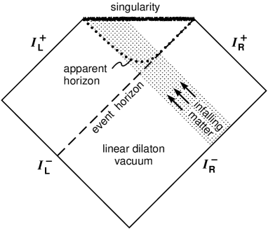
Figure 2: Penrose diagram for black hole formed by incoming matter.

In the gravitational collapse solution (13) the apparent horizon is the curve

$$x^{-}_{A}(x^{+})=-P_{+}(x^{+})\,.$$ (18)

In classical solutions the apparent horizon is always spacelike or null and along it the area of the transverse two-sphere, ${\cal A}_{A}=\exp{[-2\phi(x^{+},x^{-}_{A})]}$, is a non-decreasing function of $x^{+}$. This will no longer hold when quantum effects are included and the black hole evaporates.

The Penrose diagram in Figure 2 depicts black hole formation in the classical theory. Both the apparent horizon and the global event horizon are indicated in the figure.

3 Semi-Classical Black Hole Physics

Our analysis of the classical CGHS model has revealed physically interesting geometries including the 1+1-dimensional counterpart of a black hole formed by the gravitational collapse of matter. If a consistent quantum theory of this model can be constructed it will no doubt be considerably simpler than a theory of real gravity in 3+1 dimensions, but even the quantization of two-dimensional gravity is an ambitious goal and we will have to settle for a few modest steps in that direction here.

3.1 The Hawking Effect

In his famous 1975 paper [1] Hawking studied quantum effects of matter in the classical background geometry of a black hole formed in collapse and concluded that the black hole will emit thermal radiation as if it were a blackbody at a temperature which is proportional to its surface gravity. This effect also occurs in 1+1 dimensional black hole physics [15] and for conformally coupled matter the calculation can be carried out in a neat fashion by making use of an observation of Christensen and Fulling [23]. The argument goes as follows. The classical matter theory of the $f_{i}$ fields has a traceless conserved energy-momentum tensor but when the matter fields are quantized they give rise to a conformal anomaly,

$$\langle T_{\>\mu}^{f\>\mu}\rangle={N\over 24}R\,.$$ (19)

The left hand side is the expectation value of the trace of the matter energy-momentum tensor and on the right hand side $R$ is the curvature scalar in the classical background geometry while $N$ is the number of scalar fields in the theory, or, more generally, the central charge of the matter system. In the conformal gauge (4) the anomaly takes the form,

$$\langle T^{f}_{+-}\rangle=-{N\over 12}\partial_{+}\partial_{-}\rho\,.$$ (20)

If the quantization procedure used for the matter fields is consistent with general coordinate invariance the energy-momentum tensor will be conserved, which translates into the following pair of equations in conformal gauge,

$$\!\!\begin{array}[]{l}0=\partial_{-}\langle T^{f}_{++}\rangle+\partial_{+}\langle T^{f}_{-+}\rangle-2\partial_{+}\rho\,\langle T^{f}_{-+}\rangle\,,\\ {}\\ 0=\partial_{+}\langle T^{f}_{--}\rangle+\partial_{-}\langle T^{f}_{+-}\rangle-2\partial_{-}\rho\,\langle T^{f}_{+-}\rangle\,.\end{array}$$ (21)

Inserting the conformal gauge expression (20) for the anomaly into these equations and integrating gives

$$\!\!\begin{array}[]{l}\langle T^{f}_{++}\rangle=-{N\over 12}\bigl{[}\partial_{+}\rho\partial_{+}\rho-\partial_{+}^{2}\rho+t_{+}(y^{+})\bigr{]}\,,\\ {}\\ \langle T^{f}_{--}\rangle=-{N\over 12}\bigl{[}\partial_{-}\rho\partial_{-}\rho-\partial_{-}^{2}\rho+t_{-}(y^{-})\bigr{]}\,.\end{array}$$ (22)

The above argument is quite general as it uses only the conservation of energy-momentum and the existence of the conformal anomaly to express all the components of the anomalous energy-momentum tensor in terms of the background metric. Some further physical input is needed to fix the functions of integration $t_{\pm}$. In the case of a black hole formed in collapse this input comes in the form of boundary conditions imposed at past null infinity, stating that there is no outgoing energy flux in the initial vacuum at ${\cal I}^{-}_{L}$ and that only the classical matter energy flux is incident at ${\cal I}^{-}_{R}$.

The functions $t_{\pm}$ are intimately connected with the issue of regularization in the matter quantum theory. The energy-momentum tensor is a composite operator and its expectation value is not well defined unless we specify a normal ordering prescription with respect to some vacuum state. A choice of vacuum for the matter fields corresponds to a choice of coordinate system in that the vacuum is defined to contain no quanta with positive frequency as measured by some time variable. As a result the normal ordering prescription used to define the expectation value of the energy-momentum tensor is coordinate dependent, and observers, which are at rest in a different reference frame than the one the vacuum is defined in, will in general measure a non-vanishing energy flux in that vacuum state. The role of $t_{\pm}$ is to keep track of this coordinate dependent energy flux and their transformation under a conformal reparametrization is as follows,

$$t_{+}(x^{+})=\bigl{(}{dx^{+}\over dy^{+}}\bigr{)}^{-2}\bigl{(}t_{+}(y^{+})+{1\over 2}{\cal D}^{S}_{y^{+}}[x^{+}]\bigr{)}\,,$$ (23)

where

$${\cal D}^{S}_{y}[x]={\partial^{3}x/\partial y^{3}\over\partial x/\partial y}-{3\over 2}{(\partial^{2}x/\partial y^{2})^{2}\over(\partial x/\partial y)^{2}}$$ (24)

is the Schwarzian derivative of $x$ with respect to $y$. A similar relation holds for $t_{-}$.

We are interested in the outgoing energy flux measured by asymptotic inertial observers so we want to evaluate $t_{\pm}$ in a coordinate system $(\sigma^{+},\sigma^{-})$ where the metric is manifestly Minkowskian in the asymptotic regions near ${\cal I}^{+}_{R}$ and ${\cal I}^{-}_{R}$,

$$\sigma^{+}=\log{x^{+}}\,,\quad\sigma^{-}=-\log{(-x^{-}-P_{\infty})}\,.$$ (25)

The boundary conditions on the matter energy-momentum tensor are applied at past null infinity and imply $t_{\pm}(\tilde{\sigma}^{\pm})=0$ in a coordinate system $(\tilde{\sigma}^{+},\tilde{\sigma}^{-})$ where the metric is manifestly flat at ${\cal I}^{-}_{L}$. These coordinates are related to the $\sigma$-coordinates by

$$\tilde{\sigma}^{+}=\sigma^{+}\,,\quad e^{-\tilde{\sigma}^{-}}=e^{-\sigma^{-}}+P_{\infty}\,,$$ (26)

and by applying the transformation rule (23) one obtains

$$\!\!\begin{array}[]{l}t_{+}(\sigma^{+})=0\\ {}\\ t_{-}(\sigma^{-})={1\over 4}\bigl{(}(1+P_{\infty}e^{\sigma^{-}})^{-2}-1\bigr{)}\,.\end{array}$$ (27)

This in turn implies that there is a non-vanishing outgoing energy flux at ${\cal I}^{+}_{R}$ given by

$$\langle T^{f}_{--}\rangle={N\over 48}\bigl{(}1-(1+P_{\infty}e^{\sigma^{-}})^{-2}\bigr{)}\,.$$ (28)

The outgoing energy flux is zero at early retarded times but builds up to a fixed value and continues forever because our calculation has not taken into account the back-reaction on the geometry due to the emitted energy. The dependence on $P_{\infty}$ of the energy flux in (28) can be removed by a uniform shift of the retarded time coordinate $\sigma^{-}$ leaving an expression for the rate of Hawking radiation which is completely independent of the original incoming matter energy distribution.

We have seen that two-dimensional black holes emit energy and we would now like to determine whether the outgoing flux is in the form of thermal radiation. One way to show this is to adapt Hawking’s original calculation of Bogolioubov coefficients to the two-dimensional theory [24] but a simpler approach utilizes the fact that the matter theory at hand is a conformal field theory which allows direct calculation of correlation functions of matter fields in the outgoing radiation. Consider for example $\langle\partial_{-}f_{i}(\sigma^{-}_{1})\partial_{-}f_{j}(\sigma^{-}_{2})\rangle$ at ${\cal I}^{+}_{R}$. Since the matter fields satisfy a free wave equation we can relate this correlation function to a corresponding one evaluated in the initial vacuum at ${\cal I}^{-}_{L}$, where the $f_{i}$ are free scalar fields in Minkowski space,

$$\langle\partial_{-}f_{i}(\sigma^{-}_{1})\partial_{-}f_{j}(\sigma^{-}_{2})\rangle$$ (29)

$$={\partial\tilde{\sigma}^{-}_{1}\over\partial\sigma^{-}_{1}}\,{\partial\tilde{\sigma}^{-}_{2}\over\partial\sigma^{-}_{2}}\,{\delta_{ij}\over(\tilde{\sigma}^{-}_{1}-\tilde{\sigma}^{-}_{2})^{2}}\,.$$

In the limit of late retarded time, $\sigma^{-}\rightarrow\infty$, this becomes

$$\langle\partial_{-}f_{i}(\sigma^{-}_{1})\partial_{-}f_{j}(\sigma^{-}_{2})\rangle\sim{\delta_{ij}\over\cosh{(\sigma^{-}_{1}{-}\sigma^{-}_{2})}-1}\,,$$ (30)

which is manifestly periodic under the Euclidean time translation $\Delta\sigma^{-}\rightarrow\Delta\sigma^{-}+2\pi i$. Once the black hole has settled down after its initial formation it emits thermal radiation at a temperature $T_{H}=1/2\pi$, which is independent of the black hole mass.

It is worth noting that although the final answer (30) is perfectly regular as a function of $\Delta\sigma^{-}$, as long as the coordinate difference is not too small, the calculation nevertheless involves extremely small coordinate differences in the $\tilde{\sigma}^{-}$ frame at an intermediate stage. This appearance of extremely short coordinate distances, or equivalently very high frequencies, is common to many field theoretic calculations of the Hawking effect [1, 25].

3.2 The Semiclassical Back-Reaction

In the previous subsection we have seen energy flux from a black hole but there was no response in the background geometry. This was because we used a classical solution which could not know about the Hawking effect. As a remedy for this Callan et al. [15] proposed to add to the classical action $S_{0}$ the Polyakov-Liouville term, which is induced by quantum effects of the matter,

$$S_{1}=-{N\over 96\pi}\int d^{2}y\sqrt{-g(y)}\int d^{2}y^{\prime}\sqrt{-g(y^{\prime})}$$ (31)

$$\times R(y)G(y;y^{\prime})R(y^{\prime})\,,$$

where $G$ is a Green function for the operator $\nabla^{2}$. In conformal gauge this non-local term reduces to a local expression,

$$S_{1}=-{N\over 12\pi}\int d^{2}y\,\partial_{+}\rho\partial_{-}\rho\,,$$ (32)

but there remains a residual non-locality in the form of the functions $t_{\pm}$, which we encountered before. Fixing these functions corresponds to choosing boundary conditions for the Green function in (31).

The dilaton gravity sector of the theory also gives rise to quantum corrections to the effective action but if we take the limit of $N>>24$ the induced term (31) will dominate over other one-loop corrections and we need not be concerned with a number of thorny issues involving functional measures and reparametrization ghosts. Those problems will be addressed in Section 4 but for now we will work in the large $N$ limit.

The semiclassical CGHS equations, obtained by varying the effective action $S=S_{0}+S_{1}$, have been analyzed by a number of authors [15, 19, 22, 26, 27, 28]. They have solutions describing evaporating black holes and the back-reaction on the geometry is expected to be reliably described for most of the lifetime of black holes formed with mass $M>>N$. The CGHS model cannot be solved exactly at the semiclassical level and only permits analytical study of the onset of the evaporation process. The equations have been solved numerically to follow the evolution of the geometry [29].

3.3 The RST Model

Fortunately the semi-classical theory can be modified in such a way that explicit analytic solutions which exhibit black hole evaporation are obtained, as was first shown by Bilal and Callan [30] and de Alwis [31]. A particularly simple semiclassical model of this type was introduced by Russo, Susskind, and Thorlacius (RST) [32], who proposed to include in the effective action, in addition to the non-local term (31), the local term

$$S_{2}={N\over 96\pi}\int d^{2}y\,\sqrt{-g}\,R\phi\,,$$ (33)

which takes the form

$$S_{2}=-{N\over 12\pi}\int d^{2}y\,\phi\partial_{+}\partial_{-}\rho\,.$$ (34)

in conformal gauge. The role of this term is to restore at the semiclassical level the symmetry, generated by the conserved current $j^{\mu}=\partial^{\mu}(\rho-\phi)$, which enabled the exact solution of the classical theory. The new term in the action is manifestly covariant so it is allowed by the symmetries of the original theory and could have been included from the beginning. It has the appearance of a one-loop counterterm and therefore it does not disturb the classical physics of the model in the asymptotic region where $e^{-2\phi}>>N/24$.

The analysis of the model is simplified if we introduce new field variables for the dilaton gravity sector,

$$\!\!\begin{array}[]{l}\Omega={12\over N}e^{-2\phi}+{1\over 2}\phi-{1\over 4}\log{N\over 48}\,,\\ {}\\ \chi=\rho+{12\over N}e^{-2\phi}-{1\over 2}\phi+{1\over 4}\log{N\over 3}\,,\end{array}$$ (35)

for which the effective action $S=S_{0}+S_{1}+S_{2}$ takes the form

$$S={N\over 12\pi}\int d^{2}y\bigl{[}-\partial_{+}\chi\partial_{-}\chi+\partial_{+}\Omega\partial_{-}\Omega$$ (36)

$$+e^{2(\chi-\Omega)}+{6\over N}\sum_{i=1}^{N}\partial_{+}f_{i}\partial_{-}f_{i}\bigr{]}\,.$$

In terms of the new variables the equations of motion are

$$\!\!\begin{array}[]{l}\partial_{+}\partial_{-}f_{i}=0\\ {}\\ \partial_{+}\partial_{-}\chi=\partial_{+}\partial_{-}\Omega=-e^{2(\chi-\Omega)}\,,\end{array}$$ (37)

and the semiclassical constraint equations become

$$(\partial_{\pm}\chi)^{2}-\partial_{\pm}^{2}\chi-(\partial_{\pm}\Omega)^{2}+t_{\pm}=\tilde{T}_{\pm\pm}\,.$$ (38)

Here $\tilde{T}_{\pm\pm}$ is the observable energy-momentum flux in the asymptotic region, rescaled by a factor of $12/N$, which is appropriate in the large $N$ limit where we study black holes formed by incoming energy measured in units of $N$.

We can choose Kruskal coordinates, in which $\chi=\Omega$, and the equations of motion and constraints reduce to

$$\!\!\begin{array}[]{l}\partial_{+}\partial_{-}\Omega=-1\,,\\ {}\\ -\partial_{\pm}^{2}\Omega=\tilde{T}_{\pm\pm}-t_{\pm}\,.\end{array}$$ (39)

Notice the similarity with the classical equations (39). The matter energy-momentum tensor $\tilde{T}_{\pm\pm}$ is normal ordered with respect to the vacuum state appropriate to inertial observers in the asymptotically Minkowskian coordinates (25). The vacuum state has $\tilde{T}_{\pm\pm}=0$ and $t_{\pm}(\sigma^{\pm})=0$, which gets transformed to $t_{\pm}(x^{\pm})=1/4{x^{\pm}}^{2}$ in Kruskal coordinates under (23). The vacuum solution obtained by integrating (39) is then

$$\Omega=-x^{+}x^{-}-{1\over 4}\log{(-x^{+}x^{-})}-{1\over 2}\log{2}\,.$$ (40)

A comparison with the field redefinition (35) reveals that in this semiclassical model the dilaton field is linear, $\phi=-\sigma^{1}-{1\over 2}\log{(N/12)}$, in the vacuum solution just as in the classical theory.

Now consider a geometry with leftmoving matter incident on the vacuum from ${\cal I}^{-}_{R}$. The semiclassical solution is

$$\Omega=-x^{+}\bigl{(}x^{-}+\tilde{P}_{+}(x^{+})\bigr{)}+\tilde{M}(x^{+})$$ (41)

$$-{1\over 4}\log{(-x^{+}x^{-})}-{1\over 2}\log{2}\,,$$

where $\tilde{M}$ and $\tilde{P}_{+}$ are the moments (14) and (15) of the incoming energy flux in Kruskal coordinates, rescaled by a factor of $12/N$. Although this is a perfectly good solution of the semiclassical equations (39) its physical interpretation is problematic. The reason is that the range of values taken by $\Omega$ as a function of $x^{+}$ and $x^{-}$ is unrestricted but the field redefinition (35) is degenerate (see Figure 3), and $\Omega$ below a certain critical value $\Omega_{{\rm cr}}$, corresponds to a complex value of the original dilaton field. The critical point, where $\Omega^{\prime}(\phi)=0$, is at $\phi_{{\rm cr}}=-{1\over 2}\log{(N/48)}$ and $\Omega_{{\rm cr}}={1\over 4}$.

Figure 3: The field redefinition from $\phi$ to $\Omega$ is not one-to-one.

The existence of this critical value of the dilaton field has important implications. By using the equations of motion (37) written in terms of $\rho$ and $\phi$ one can express the spacetime curvature as

$$R={4\over 1-{N\over 48}e^{2\phi}}\bigl{(}1-(\nabla\phi)^{2}\bigr{)}\,,$$ (42)

and we see that in general the curvature will diverge where $\phi=\phi_{{\rm cr}}$, even if the solution for $\chi$ and $\Omega$ is perfectly regular there. Gravitational quantum corrections are strong in this model when the dilaton field is near its critical value. This can be seen by defining the two-component vector

$$\Phi=\left[\begin{array}[]{c}\phi\\ \rho\end{array}\right]\,,$$ (43)

and assembling the kinetic terms in the full effective action $S=S_{0}+S_{1}+S_{2}$ into $(\partial_{+}\Phi)M(\partial_{-}\Phi)$. The role of gravitational coupling is played by

$$(-\det{M})^{-1/4}\sim(e^{-2\phi}-{N\over 48})^{-1/2},$$ (44)

which goes to infinity as $\phi\rightarrow\phi_{{\rm cr}}$.

It is tempting to ignore the problem of unphysical values of $\Omega$ and simply define the semiclassical theory in terms of the effective action (36) for $\chi$ and $\Omega$. Such a theory has the appropriate classical limit by construction and the smooth behavior of $\chi$ and $\Omega$ in the strong coupling region of the original theory in effect resolves the classical singularity. Unfortunately this approach is undermined by an instability. The incoming matter excites the system from its vacuum configuration and Hawking radiation is emitted to ${\cal I}^{+}_{R}$. The mismatch between inertial coordinates at ${\cal I}^{+}_{R}$ and ${\cal I}^{-}_{L}$ is given by (26), with $P_{\infty}$ replaced by $\tilde{P}_{\infty}$, and the calculation of the Hawking flux at ${\cal I}^{+}_{R}$ proceeds in the same manner. Although the semiclassical solution exhibits a back-reaction effect on the geometry due to the Hawking emission there is nothing to turn the outgoing flux off when the emitted energy exceeds the total incoming energy and the Bondi mass measured at ${\cal I}^{+}_{R}$ goes to negative infinity at late times.

In order to avoid these problems of unphysical $\Omega$ values and negative energy instability, Russo et al. [32] interpreted the curve $\Omega=\Omega_{{\rm cr}}$ as the analog of the origin of radial coordinates in higher dimensional gravity, beyond which solutions should not be continued, and proposed ‘phenomenological’ boundary conditions for $\Omega$,

$$\partial_{+}\Omega\big{|}_{\Omega=\Omega_{{\rm cr}}}=0=\partial_{-}\Omega\big{|}_{\Omega=\Omega_{{\rm cr}}}\,,$$ (45)

which ensure that the spacetime curvature remains finite at the critical curve where it is timelike. This turns out to stabilize the semiclassical evolution, which is perhaps not surprising since negative energy configurations typically have naked singularities and the above boundary conditions implement a form of cosmic censorship in the two-dimensional theory.

It should be noted, however, that these boundary conditions for $\Omega$ are not the most general ones allowed and they do not imply boundary conditions for the matter fields, which is a drawback if we want to discuss the quantum state of the outgoing matter in connection with the information paradox. It was initially claimed [32] that the RST boundary conditions on $\Omega$ would be compatible with Dirichlet or Neumann boundary conditions on the $f_{i}$ but it was later realized that this is not the case [34, 35], and (45) may in fact not be realizable as the semiclassical limit of any consistent quantum mechanical boundary conditions. In Section 4 we will discuss alternative choices of boundary conditions [36, 37, 38], which are compatible with simple reflecting conditions on the matter fields, but these models are somewhat more complicated than the RST model and the analysis of the semiclassical solutions less transparent. We will therefore explore the physical picture presented in the RST model before moving on to other models.

3.4 Semiclassical Black Holes

Let us first consider the static solutions of the semiclassical equations (39) subject to the boundary conditions (45),

$$\Omega=-x^{+}x^{-}-{(1-a)\over 4}\log{(-x^{+}x^{-})}$$ (46)

$$+M+{a\over 4}+{(1-a)\over 4}\log{({1-a\over 4})}\,.$$

These static geometries are characterized by two parameters. One is proportional to the asymptotic energy density, $a/4=\tilde{T}_{++}=\tilde{T}_{--}=$ as $\sigma^{1}\rightarrow\infty$, and the other one $M$, will be referred to as the mass even if the canonical ADM mass diverges for geometries with a non-vanishing asymptotic energy density.

The solution with $a=0$ and $M=0$ is the linear dilaton vacuum (40), for $a=0$ and $M>0$ it is a ‘quantum kink’ solution with a singular horizon at $x^{+}x^{-}=0$ [26, 27], and for $a=0$ and $M<0$ it has a naked singularity.

A solution with $0<a<1$ and $M=0$ corresponds to a heat bath at a temperature $T=a/2\pi$. A semiclassical black hole emits Hawking radiation and a static configuration can only exist if the black hole is in equilibrium with a heat bath at a temperature equal to the Hawking temperature $T_{H}=1/2\pi$. This is described by a static solution with $a=1$ and $M>0$, which has a spacelike singularity at $x^{+}x^{-}=M$ and non-singular event horizon at $x^{+}x^{-}=0$. Notice that since the boundary curve $\Omega=1/4$ is spacelike in the static black hole geometries they are determined without applying the boundary conditions (45).

The black hole temperature is independent of the mass parameter so that the specific heat is infinite. Random fluctuations in the thermal flux of energy at the horizon will therefore cause the black hole mass to slowly increase or decrease with time [35, 39]. In ordinary systems, which have a finite positive specific heat, such fluctuations are stabilized by a response in the temperature of the system. A momentary increase (decrease) in the energy of a system in equilibrium with a heat bath causes an increase (decrease) in the temperature of the system, which in turn causes heat to flow to (from) the bath. In the case at hand, the black hole temperature does not respond to the energy fluctuation and there is no restoring effect to maintain a balance. With time the black hole mass will therefore random walk away from its original value. The semiclassical equations do not incorporate this thermal effect but physically the one-parameter family of distinct static black hole solutions should be replaced by a single ensemble which includes black holes of arbitrary mass.

We now turn our attention to dynamical solutions of the semiclassical equations subject to the boundary conditions (45). The semiclassical geometry can be explicitly determined everywhere in spacetime and expressed in a relatively compact form,

$$\Omega=-x^{+}\bigl{(}x^{-}+\tilde{P}_{+}(x^{+})\bigr{)}+\tilde{M}(x^{+})$$ (47)

$$-\tilde{M}\bigl{(}x^{+}_{b}(x^{-})\bigr{)}-{1\over 4}\log{\bigl{(}x^{+}/x^{+}_{b}(x^{-})\bigr{)}}\,.$$

Here $x^{+}_{b}(x^{-})$ is the $x^{+}$ value of the point on the boundary curve $\Omega=\Omega_{{\rm cr}}$ from which the reflected signal propagates to $(x^{+},x^{-})$ as shown in Figure 4.

Figure 4: Kruskal diagram for a black hole formed by incoming matter in the semiclassical theory.

The qualitative behavior of the semiclassical solution (47) depends on the incoming matter energy. There is a threshold energy flux required for black hole formation, which coincides with the rate of Hawking emission from a black hole. As long as the incoming energy flux remains below threshold, $\tilde{T}_{++}<1/4{x^{+}}^{2}$, the boundary curve, defined by $\Omega(x^{+}_{b},x^{-}_{b})=1/4$, will be timelike and its shape given by

$$x^{-}_{b}=-\tilde{P}_{+}(x^{+}_{b})-{1\over 4x^{+}_{b}}\,.$$ (48)

Consider a geometry where the incoming energy flux tapers off at early and late times and always remains below threshold. As $x^{+}\rightarrow\infty$ and $x^{-}\rightarrow 0$ the solution (47) approaches the linear dilaton vacuum (40) up to a uniform shift of $x^{-}$ by $\tilde{P}_{\infty}$. By combining the boundary conditions (45) and the constraint equations in (39) one can obtain the outgoing energy flux due to a given incoming matter energy profile. The total outgoing energy can then be computed by integrating the outgoing flux in the asymptotically inertial coordinate system (25) over all retarded time (remembering to take into account the anomalous transformation properties of $t_{-}$ when passing from the Kruskal coordinate system) and one finds that it equals $\tilde{M}_{\infty}$, the total incoming energy. The RST boundary conditions thus respect overall energy conservation even if it is not manifest.

Now consider the case when the incoming energy flux becomes larger than the threshold value at some point. Then the boundary curve becomes spacelike and boundary conditions can no longer be applied there. A spacelike segment of the boundary is a curvature singularity. It forms inside a region of future trapped points which is bounded on the outside by an apparent horizon, located where $\partial_{+}\phi=0$, as shown in Figures 4 and 5.

The apparent horizon curve $(x^{+}_{a},x^{-}_{a})$ satisfies

$$x^{-}_{a}=-\tilde{P}_{+}(x^{+}_{a})-{1\over 4x^{+}_{a}}\,,$$ (49)

which is the same equation as (48), which determined the timelike boundary, but the two apply under different circumstances as the apparent horizon only exists for those values of $x^{+}$ where the boundary curve is spacelike and (48) does not hold. The apparent horizon curve is itself spacelike whenever the incoming energy flux is above threshold and the black hole is gaining mass. Once the incoming flux falls below threshold there is a net loss of energy from the black hole due to Hawking emission and the apparent horizon becomes timelike. If the incoming flux remains below threshold for a sufficiently long time the apparent horizon will run into the spacelike singularity. At the black hole endpoint, which is denoted by $E$ in Figure 4, the boundary curve becomes timelike again and the boundary conditions (45) can be applied.

The solution in the causal future of the black hole endpoint matches continuously onto the evaporating black hole solution across the line segment $\{x^{-}=x^{-}_{E},x^{+}>x^{+}_{E}\}$, but the match is not smooth. The derivative $\partial_{-}\Omega$ is discontinuous there by an amount which by the constraint equations in (39) corresponds to an outgoing shock wave carrying a small negative energy. The fact that negative energy is carried out from the endpoint is perhaps strange but it is not very serious. Energy density is not positive definite in quantum theories and global energy positivity is not violated by this negative energy ‘thunderpop’ whose energy is bounded by the analog of the Planck scale in this theory, $|\tilde{T}_{--}(\sigma^{-})|<1/4$.

The expression for spacetime curvature (42) takes a simple form on the apparent horizon curve

$$R={4\over 1-{N\over 48}e^{2\phi}}\,,$$ (50)

and it follows that the curvature diverges on the apparent horizon as it approaches the black hole singularity. The apparent horizon of an evaporating black hole is visible from future null infinity and the diverging curvature means that the endpoint of evaporation is a naked singularity. Cosmic censorship is therefore violated but by adopting the boundary conditions (45) after the evaporation is complete the violation is kept to a minimum.

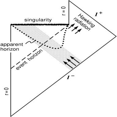
Figure 5: Penrose diagram for a black hole formed by incoming matter in the semiclassical theory.

Consider, for concreteness, a geometry where a black hole is formed by an incoming energy flux which is above threshold for a while but is then turned off at some finite value of $x^{+}$. The associated Penrose diagram is shown in Figure 5. In this case, the black hole endpoint occurs in a region where there is no incoming energy flux and once the thunderpop has been emitted the solution (47) reduces to the linear dilaton vacuum (40) up to the usual shift of $x^{-}$ by $\tilde{P}_{\infty}$. The outgoing energy flux in Hawking radiation takes exactly the same form as in (28) except that it shuts off once the thunderpop arrives at ${\cal I}^{+}_{R}$. In a classical background geometry the rate of Hawking emission did not depend at all on the incoming energy profile. We are doing somewhat better here in that the radiation only lasts for a time which is proportional to the original black hole mass, so that energy is conserved, but apart from that the Hawking energy flux reflects none of the detailed structure of the incoming matter distribution.

Since we do not have boundary conditions on the matter fields we cannot make precise statements about information loss at this stage. On the other hand, since all the incoming matter that arrives between $x^{+}=x^{+}_{b}(x^{-}_{E})$ and $x^{+}=x^{+}_{E}$ will pass through the global event horizon of the black hole without any chance of reflecting off the boundary, it seems clear that no local boundary conditions on the $f_{i}$ can prevent information from entering the black hole in this model.

We would be able to make a stronger statement if we could impose simple reflecting boundary conditions, either Dirichlet or Neumann, on the matter fields and appeal to the standard lore [40] on quantum fields reflecting off moving mirrors. The problem is that the RST boundary conditions (45) are incompatible with reflecting boundary conditions for the matter fields [34, 35] and it is therefore in general inconsistent to use the above semiclassical solutions as background geometries for quantized matter fields.

The incompatibility can be seen by comparing the outgoing energy flux found for a semiclassical solution (47) in the low-energy sector of the RST model to the energy flux that would be obtained if the timelike boundary curve were replaced by a mirror that moved along the same trajectory. It is straightforward to show that the two disagree and that the disagreement becomes particularly pronounced in the limit when the incoming matter energy flux approaches the threshold for black hole formation [35]. If we go beyond the the threshold and let a black hole form then the problem gets even worse. In this case the reflecting boundary is disconnected as it jumps from $(x^{+}_{b},x^{-}_{E})$ to the black hole endpoint at $(x^{+}_{E},x^{-}_{E})$. A disconnected mirror trajectory gives rise to an infinite burst of outgoing energy at the discontinuity [41] instead of the relatively benign thunderpop found in the RST model.

This incompatibility is a stumbling block that confounds the quantization of the RST model. Alternate boundary conditions for dilaton gravity, which are consistent with Dirichlet or Neumann conditions on the matter fields, have been considered [36, 37, 38], and will be discussed below.

4 Conformally Invariant Models

So far, we have considered quantum effects of the matter theory but treated the dilaton and conformal factor as classical fields whose equations of motion receive correction terms due to the quantization of matter fields. While the contribution from the matter to the effective action dominates over other one-loop term in the large $N$ limit we must nevertheless consider a more systematic quantization of the complete theory if we wish to address fundamental questions such as information loss. Another reason to go beyond the large $N$ approximation is that it breaks down near the singularity inside a black hole and at the endpoint of black hole evaporation. These issues have been addressed by a number of authors [30, 31, 42, 43, 44]. We will adopt the conventions of [43] in our discussion.

4.1 Conformal Gauge Quantization

The quantum theory of dilaton gravity coupled to scalar fields is formally defined in terms of the functional integral

$${\cal Z}=\int{\cal D}(g,\phi,f_{i})\,e^{iS_{0}}\,.$$ (51)

In order to be meaningful this expression requires a prescription for gauge fixing, regularization, and renormalization. It is usually assumed that some covariant non-perturbative method of regularizing the continuum theory exists although at present no such method is available. Instead we shall rely on a procedure which is analogous to old-fashioned methods of regularization and renormalization in gauge theories. By this procedure the theory is first regularized in a non-covariant way and then one compensates for the resulting non-invariance by allowing the effective Lagrangian to contain terms that are not gauge invariant. At the end of the day the gauge symmetry is re-imposed through Ward identities, which constrain the added terms. A version of this method applied to two-dimensional gravity is as follows [45].

The first step is gauge fixing. We have to remove the over-counting of metrics due to general coordinate invariance. This is achieved by fixing some reference metric $\hat{g}_{ab}$, which could for example be the flat Minkowski metric, and then choosing coordinates such that the physical metric is conformal to the reference metric,

$$g_{ab}=e^{2\rho}\hat{g}_{ab}\,.$$ (52)

In two spacetime dimensions such a coordinate system can always be found locally. The original path integral over metrics is replaced by an integral over the conformal factor $\rho$ along with the usual anticommuting Faddeev-Popov ghosts.

The next step is regularization. The theory has ultraviolet divergences which must be regularized in order to define the gauge fixed path integral. A non-perturbative regulator could for example be introduced by discretizing the spacetime so that there is a shortest length, as measured by the reference metric,

$$\hat{g}_{ab}\,\delta x^{a}\,\delta x^{b}>\varepsilon\,,$$ (53)

where $\delta x^{a}$ is the element connecting nearest neighbor lattice points and $\varepsilon$ tends to zero as the cutoff is removed. A more covariant method would refer the cutoff to the physical metric $g_{ab}$, but then the regularization would depend on the conformal factor, which is one of the fields being integrated over, and the regularized path integral would not have a concrete definition.

The final step involves renormalization. Performing the path integral over short distance fluctuations of the conformal factor, dilaton, and matter fields generates various interaction terms, involving $\rho$, $\phi$, and $f_{i}$, in the effective Lagrangian. In general these terms depend on the arbitrarily chosen reference metric $\hat{g}_{ab}$ and therefore the effective action will not be manifestly covariant. On the other hand, the original theory is assumed to be invariant under general coordinate transformations so we must impose on the renormalized theory that the value of the path integral does not depend on the choice of reference metric. This can be achieved by, first of all, arranging the terms in the effective action to be covariant with respect to $\hat{g}_{ab}$. This does not restrict the possible couplings but merely labels them by their transformation properties under reparametrizations of the reference system. Then we impose that the path integral remains invariant under the transformation

$$\hat{g}_{ab}\rightarrow e^{2\delta\alpha}\hat{g}_{ab}\,\quad\rho\rightarrow\rho-\delta\alpha\,,$$ (54)

which leaves the left hand side of (52) invariant. This condition translates into the restriction that the beta-functions of all the couplings in the theory must vanish. In other words, the gauge fixed theory must be an exact fixed point of the renormalization group in order to maintain the original general covariance. Since the Faddeev-Popov ghosts contribute $-26$ to the conformal anomaly the theory of the remaining fields should be a $c=26$ conformal field theory.

We are thus led to consider a reparametrization invariant field theory in two dimensions, where the action can a priori include terms with an arbitrary functional dependence on the $N+2$ fields $X^{\mu}=(\rho,\phi,f_{i})$, and with any number of derivatives acting on the fields,

$$S=-{1\over 2\pi}\int d^{y}\sqrt{-\hat{g}}\bigl{[}T(X)+{1\over 2}\hat{R}\,\Phi(X)$$ (55)

$$+\hat{g}^{ab}\hat{\nabla}_{a}X^{\mu}\hat{\nabla}_{b}X^{\nu}G_{\mu\nu}(X)+\ldots\bigr{]}\,.$$

We have only written terms of scaling dimension zero and two but in general there is an infinite sequence of possible couplings involving any number of derivatives of the $X^{\mu}$ and higher powers of $\hat{R}$, the curvature of the reference metric.

This class of theories has been extensively studied in string theory where the action (55) describes strings in background fields in $N+2$ dimensional target space. The beta-function equations, which implement conformal invariance of the two-dimensional theory, have the form of field equations in target space. In order to completely specify the two-dimensional theory we need to give initial data for all the beta-function equations and then solve them. Exact solutions are only available under very special circumstances and in the general case we can at best hope to find a small parameter for a perturbation expansion. In the case at hand, we have the loop expansion parameter $e^{2\phi}$ of the dilaton gravity which is small in the classical limit.

4.2 Models for Black Hole Physics

The conformal invariance condition places restrictions on the possible two-dimensional effective theories that correspond to generally covariant theories of gravity, but there is still an infinite class of allowed theories. The different theories correspond to different physical systems and we can narrow the field down by imposing some further physical restrictions, which are appropriate to the application we have in mind.

First of all, since we are interested in studying black holes we require our effective theory to reduce to the classical CGHS theory in the limit $e^{2\phi}\rightarrow 0$. As a corollary to this requirement we also want the linear dilaton vacuum, or a close relative, to be a solution of the effective theory so that we can study gravitational collapse as in the CGHS model.

As a further requirement we want the leading order corrections in powers of $e^{2\phi}$ to give rise to the appropriate semiclassical behavior of black holes, i.e. Hawking radiation and its back-reaction on the geometry. A subtle issue, which has led to persistent confusion in the literature, arises in this context. The Hawking radiation should consist only of matter fields, whereas the non-propagating fields of the theory, $\rho$, $\phi$, and the Faddeev-Popov ghosts, should not contribute to the outgoing energy flux. We have already encountered the Polyakov-Liouville term (31), which is responsible for the matter contribution to the Hawking effect, and naively one would expect analogous terms arising as one-loop contributions from the path integral over $\rho$, $\phi$, and the ghosts. The coefficient in front of the Polyakov-Liouville term in the effective action would then be proportional to $N+2-26$ instead of $N$ and this would lead to the unphysical conclusion that the rate of Hawking evaporation is not proportional to the number of available channels $N$ but rather $N-24$. This can be ignored in the large $N$ limit, as we did in Section 3, but for finite $N$, and $N<24$ in particular, this is not acceptable.

This problem was solved at the one-loop level by Strominger [46] who introduced local covariant counterterms into the effective action to decouple the non-propagating modes from the Hawking radiation. His choice of counterterms was motivated by the observation that the natural metric that defines the functional measure for $\rho$, $\phi$, and the ghost fields in the path integral involves $\rho-\phi$ rather than just $\rho$. This can be seen by comparing the kinetic terms of the dilaton gravity part of the classical action (1) to the matter kinetic terms. The resulting one-loop contribution to the effective action due to $\rho$, $\phi$, and the ghosts takes the form

$$S_{gh}={24\over 12\pi}\int d^{2}y\,\partial_{+}(\rho-\phi)\partial_{-}(\rho-\phi)$$ (56)

in conformal gauge. The $\partial_{+}\rho\partial_{-}\rho$ part is non-local in a general gauge and combines with the matter contribution to the Polyakov-Liouville counterterm of the model but the other terms in (56) correspond to local counterterms involving $R\phi$ and $(\nabla\phi)^{2}$. The ultimate justification for this choice comes when we consider semiclassical black holes in our effective theory and determine their rate of Hawking evaporation.

To summarize, we will restrict the form of our effective action to be such that it defines a $c=26$ conformal field theory and in the limit $e^{2\phi}\rightarrow 0$ the leading order terms reduce to the classical CGHS model (1), corrected by (32) and (56). This requires the target space fields that appear in (55) to have the following limiting behavior [43], up to $O(e^{2\phi})$ terms,

$$\!\!\begin{array}[]{ll}G_{\rho\rho}\sim-\gamma\,,&G_{\rho\phi}\sim 2e^{-2\phi}{-}2,\\ {}&{}\\ G_{\phi\phi}\sim-4e^{-2\phi}+2\,,&G_{ii}\sim{1\over 2}\,,\\ {}&{}\\ \Phi\sim-2e^{-2\phi}{-}4\phi{-}2\gamma\rho,&{}\\ {}&{}\\ T\sim-4e^{2\rho-2\phi}+O(1)\,,&{}\end{array}$$ (57)

where we have defined $\gamma=(N-24)/12$.

As a final requirement on our effective action we would like to impose the ‘theoretician’s condition’ that it be possible to explicitly solve the semiclassical equations of the model. This is clearly not a physical requirement but if it can be met it allows detailed analytical analysis of the semiclassical physics, which enhances our understanding of the model, and further down the road it may also simplify some technical steps involved in its quantization.

4.3 A Soluble Model

It turns out to be possible to satisfy all the above requirements and construct a conformally invariant model, where the semiclassical equations can be solved exactly, as was first shown independently by Bilal and Callan [30] and de Alwis [31]. Consider the effective action

$$S={1\over\pi}\int d^{2}y\bigl{[}-\gamma\partial_{+}X\partial_{-}X+\gamma\partial_{+}Y\partial_{-}Y$$ (58)

$$+e^{2(X-Y)}+{1\over 2}\sum_{i=1}^{N}\partial_{+}f_{i}\partial_{-}f_{i}\bigr{]}\,,$$

where the field variables $X$ and $Y$ are related to the conformal factor and dilaton as follows,

$$\!\!\begin{array}[]{l}X=\rho+{1\over\gamma}(e^{-2\phi}+2\phi)\,,\\ {}\\ Y=-{1\over\gamma}\int d\phi\sqrt{4e^{-4\phi}-4(\gamma{+}2)e^{-2\phi}+2(\gamma{+}2)}\,.\end{array}$$ (62)

Substituting $X$ and $Y$ into this action leads to the classical CGHS action (1) corrected by the one-loop terms (32) and (56) along with additional potential terms which are subleading in the loop expansion parameter $e^{2\phi}$. The $X,Y$ theory is identical to the $\chi,\Omega$ theory of the RST model (up to some numerical factors) but the field redefinition to $\rho$ and $\phi$ variables differs significantly and this has important consequences for the physics.

The gravitational part of the energy-momentum tensor is given by

$$T^{g}_{\pm\pm}=\gamma(\partial_{\pm}Y\partial_{\pm}Y-\partial_{\pm}X\partial_{\pm}X+\partial^{2}_{\pm}X)\,,$$ (64)

and together with the matter part it generates two independent $c=26$ Virasoro algebras.

The semiclassical equations of motion of this theory are obtained by varying the action (58) and up to factors of $\gamma$ they are identical to the equations of motion (37) of the RST model. As before, we can work in Kruskal gauge, $X=Y$, and express the general static solution in terms of two parameters,

$$Y=-{1\over\gamma}x^{+}x^{-}+(p-{1\over 4})\log{(-x^{+}x^{-})}+{\mu\over\gamma}\,.$$ (65)

The vacuum configuration has $\mu=0$ and $p=-1/2\gamma$ [43]. In order to see why this choice of $p$ is natural it is instructive to evaluate the gravitational part of the energy-momentum tensor for the vacuum configuration in asymptotically Minkowskian coordinates, which are related to the Kruskal coordinates by $s^{\pm}=\pm\log{x^{\pm}}$. The result is

$$T^{g}_{++}(s^{+})={1\over 2}\,,$$ (66)

along with a similar expression for $T^{g}_{--}$. The non-vanishing right hand side cancels agains a ghost energy flux, $T^{gh}_{++}=2\bigl{(}\partial_{+}(\rho-\phi)\bigr{)}^{2}$, which is included in $T^{g}_{++}$ on the left hand side of (66).

This choice of $p$ is also the only one which leads to the correct rate of Hawking evaporation of a black hole formed by collapse of matter into the vacuum [38]. To see that, keep the parameter $p$ arbitrary for the time being and consider a dynamical solution with leftmoving matter incident on the vacuum from ${\cal I}^{-}_{R}$,

$$Y=-{1\over\gamma}x^{+}\bigl{(}x^{-}+P_{+}(x^{+})\bigr{)}+{1\over\gamma}M(x^{+})$$ (67)

$$+(p-{1\over 4})\log{(-x^{+}x^{-})}\,.$$

The evaporation rate can be obtained by transforming to the inertial coordinate system (25) at ${\cal I}^{+}_{R}$ and evaluating the Bondi mass [15],

$$m(\sigma^{-})=2e^{\sigma^{+}-\sigma^{-}}(\delta\rho+\partial_{+}\delta\phi-\partial_{-}\delta\phi)\,.$$ (68)

Here $\delta\rho$ and $\delta\phi$ are the deviations of $\rho$ and $\phi$ from their vacuum values in (67). After some algebra one finds

$$m(\sigma^{-})=M_{\infty}+(p-{1\over 4})\gamma\bigl{[}\log{(1{+}P_{\infty}e^{\sigma^{-}})}$$ (69)

$$\qquad+{P_{\infty}\over P_{\infty}+e^{\sigma^{-}}}\bigr{]}.$$

If we choose $p=-1/2\gamma$ then the Bondi mass decays at a rate

$${dm\over d\sigma^{-}}=-{N\over 48}\bigl{(}1-(1+P_{\infty}e^{\sigma^{-}})^{-2}\bigr{)}\,,$$ (70)

which is indeed proportional to the number of matter fields. We have successfully removed the non-propagating modes from the Hawking radiation at the semiclassical level. There is, however, a potential conflict here with the no-ghost theorem, which has not been addressed.

4.4 Conformally Invariant Boundary Conditions

A closer examination of the expression (69) reveals a disastrous instability. If we evaluate it at late retarded times, $\sigma^{-}\rightarrow+\infty$, we find that $m(\sigma^{-})$ goes to minus infinity. The vacuum is unstable under arbitrarily small perturbations. This is of course the same disaster we encountered previously in the RST model. In that case it was avoided by restricting the range of the $\Omega$ field variable and imposing the RST boundary conditions at $\Omega=\Omega_{{\rm cr}}$.

We could adopt the same strategy here but there is a price to pay. If the range of $\Omega$ is restricted the functional integral does not define a conventional quantum field theory and it is unknown how to carry it out in a manner consistent with general covariance. We did not worry about this problem in Section 3 since we were only trying to solve semiclassical equations but it would have to be faced if we wanted to carry out a quantization of the RST model. Furthermore, as we noted before, the boundary conditions (45) on $\Omega$ appear to be incompatible with simple quantum mechanical boundary conditions on the matter fields.

An alternate procedure [36, 37, 38], is to place no restriction on the field values of $Y$ but impose boundary conditions on all fields in the theory along a timelike curve $x^{+}x^{-}=constant$. We can interpret this curve as the origin of radial coordinates $r=0$ from the point of view of a higher-dimensional theory. If we define $s^{\pm}=\pm\log{x^{\pm}}$ then the boundary curve $x^{+}x^{-}=constant$ is at a constant value of the spatial coordinate $s^{1}=s^{1}_{0}$.

Our boundary conditions need to satisfy a number of physical requirements. First of all, they should be consistent with the conformal symmetry of the bulk theory in order to ensure general covariance and energy conservation. Our second requirement is that the vacuum configuration of the bulk theory, or a close cousin, must be compatible with the boundary conditions. If the nature of the vacuum is greatly altered it can be difficult to interpret the physics of the model in terms of black holes. Finally, the boundary conditions should effect a cure of the negative energy instability of the bulk theory. We will be able to achieve stability under small perturbations, which is enough to allow the perturbative construction of a low-energy $S$-matrix for asymptotic observers. Large incoming pulses will, however, still produce low values of $Y$ and destabilize the system.

Our analysis will be semiclassical in that we treat $X$ and $Y$ as c-number fields when we impose the boundary conditions. It is presumably possible to modify the boundary conditions order by order in the loop expansion to maintain conformal invariance, or even define an exact boundary conformal field theory, but this is beyond the scope of our discussion.

The semiclassical approximation is not always reliable, but corrections to it can be systematically suppressed by taking the large $\gamma$, i.e. large $N$, limit. In taking this limit $2\tilde{X}=2X-\log{\gamma}$ and $\tilde{T}^{f}_{\pm\pm}={1\over\gamma}T^{f}_{\pm\pm}$ are held fixed. The gravitational part of the semiclassical action (58) becomes

$$S_{g}={\gamma\over\pi}\int d^{2}y\bigl{[}-\partial_{+}\tilde{X}\partial_{-}\tilde{X}+\partial_{+}Y\partial_{-}Y$$ (71)

$$\>+e^{2(\tilde{X}-Y)}\bigr{]}\,,$$

and the constraints can be written

$$\partial_{\pm}Y\partial_{\pm}Y-\partial_{\pm}\tilde{X}\partial_{\pm}\tilde{X}+\partial_{\pm}\partial_{\pm}\tilde{X}+\tilde{T}^{f}_{\pm\pm}=0\,.$$ (72)

In $s$-coordinates the vacuum solution of the bulk theory takes the simple form

$$\!\!\begin{array}[]{l}Y=\exp{(2s^{1})}-{1\over 2}\,s^{1}\,,\\ {}\\ \tilde{X}=\exp{(2s^{1})}+{1\over 2}\,s^{1}\,.\end{array}$$ (73)

Since the boundary is a straight line in this coordinate system, boundary conformal invariance is equivalent to [48]

$$\tilde{T}_{++}(s^{0},s^{1}_{0})=\tilde{T}_{--}(s^{0},s^{1}_{0})\,,$$ (74)

where $\tilde{T}$ is the total energy-momentum tensor for all fields. If either Dirichlet or Neumann boundary conditions are imposed on the matter fields,

$$\partial_{+}f_{i}(s^{0},s^{1}_{0})\pm\partial_{-}f_{i}(s^{0},s^{1}_{0})=0\,,$$ (75)

then the boundary condition (74) implies

$$\!\!\begin{array}[]{l}\partial^{2}_{+}\tilde{X}-\partial_{+}\tilde{X}\partial_{+}\tilde{X}+\partial_{+}Y\partial_{+}Y\\ {}\\ =\partial_{-}^{2}\tilde{X}-\partial_{-}\tilde{X}\partial_{-}\tilde{X}+\partial_{-}Y\partial_{-}Y\,.\end{array}$$ (76)

A simple semiclassical solution of this equation is given by

$$\!\!\begin{array}[]{l}Y=Y_{0}\,,\\ {}\\ \partial_{+}\tilde{X}-\partial_{-}\tilde{X}=Ae^{\tilde{X}-Y_{0}}\,,\end{array}$$ (77)

where $A$ and $Y_{0}$ are constants. More general solutions can be found but we will only consider this example here.

Insisting that the vacuum solution (73) be compatible with the boundary conditions determines the parameters $A$ and $Y_{0}$ in terms of $s^{1}_{0}$, the location of the boundary. The constraint on $Y_{0}$ follows directly from the $Y$ boundary condition in (77),

$$Y_{0}=\exp{(s^{1}_{0})}-{1\over 2}s^{1}_{0}\,,$$ (78)

and the $\tilde{X}$ boundary condition is satisfied by the vacuum solution only if

$$A=2\cosh{(s^{1}_{0}+\log{2})}\,.$$ (79)

Note that $A\geq 2$ for all values of $s^{1}_{0}$, which means that vacuum compatibility does not allow the theory to be analyzed perturbatively in the strength of the boundary interaction. For a given allowed value of $A$ there are two values of $s^{1}_{0}$ consistent with (79), but it turns out that only one of them makes the vacuum stable under small incoming energy perturbations.

4.5 A Dynamical Boundary Curve

A boundary condition imposed at fixed $s^{1}$ restricts the left and right conformal invariance to a diagonal subgroup. Separate left and right invariance can be regained, however, at the price of allowing the boundary to follow a general trajectory, described by an equation $y_{b}^{-}(y^{+})=y^{-}$. Holding $Y$ fixed along the boundary implies

$$u^{-1}\partial_{+}Y+u\,\partial_{-}Y=0\,,$$ (80)

where

$$u(y^{+})\equiv\bigl{(}\frac{\partial y_{b}^{-}}{\partial y^{+}}\bigr{)}^{1/2}\,,$$ (81)

and $(u^{-1},u)$ is a tangent vector to the boundary curve in the $y$-coordinate system. Neumann or Dirichlet conditions on the matter fields become

$$u^{-1}\partial_{+}f_{i}\pm u\,\partial_{-}f_{i}=0\,,$$ (82)

for a general boundary curve and the boundary condition on $X$ in (77) becomes

$$u^{-1}\partial_{+}X-u\,\partial_{-}X=Ae^{X-Y_{0}}+u^{-2}\partial_{+}u\,.$$ (83)

The last term arises because $X$ contains the conformal factor and does not transform as a scalar under a change of coordinates.

By acting on both sides of (83) with the operator $u^{-1}\partial_{+}+u\partial_{-}$, which generates translations along the boundary, we obtain

$$\!\!\begin{array}[]{l}u^{-2}(\partial_{+}^{2}X-\partial_{+}X\partial_{+}X)\\ {}\\ =u^{2}(\partial^{2}_{-}X-\partial_{-}X\partial_{-}X)-u^{-1}\partial_{+}^{2}(u^{-1})\,.\end{array}$$ (84)

This identity, together with the $Y$ boundary condition (80), can be used to relate the components of the gravitational stress tensor at a general boundary curve, that

$$u^{-2}\tilde{T}^{g}_{++}=u^{2}\tilde{T}^{g}_{--}-u^{-1}\partial_{+}^{2}(u^{-1})\,.$$ (85)

The last term is familiar from the study of moving mirrors [40]. It vanishes in “straight line” gauges for which $u$ is constant.

The dynamics of the boundary is governed by an ordinary differential equation. We find it convenient to derive it in Kruskal gauge, where $X=Y$ and the boundary conditions (80) and (83) can be combined into

$$2u^{-1}\partial_{+}Y=A+u^{-2}\partial_{+}u\,.$$ (86)

Multiplying by $u$ and then differentiating along the boundary, one obtains

$$2\partial_{+}^{2}Y+2u^{2}\partial_{-}\partial_{+}Y=A\partial_{+}u+\partial_{+}^{2}\log{u}\,.$$ (87)

The following relations hold for a general solution of the equations of motion in Kruskal gauge,

$$\!\!\begin{array}[]{l}\partial_{+}Y=-\bigl{(}x^{-}+\tilde{P}_{+}+\frac{1}{4x^{+}}\bigr{)}\,,\\ {}\\ \partial^{2}_{+}Y=-\tilde{T}^{f}_{++}+\frac{1}{4x^{+2}}\,,\\ {}\\ \partial_{-}\partial_{+}Y=-1\,.\end{array}$$ (88)

Substituting into (87) leads to

$$\partial_{+}^{2}\log{u}+A{\partial_{+}u}+2u^{2}-\frac{1}{2{x^{+}}^{2}}=-2\tilde{T}^{f}_{++}.$$ (89)

An alternate form of this boundary differential equation is obtained by transforming to the $s$-coordinate system and defining $\omega(s^{+})=s^{+}+\log{u}$. This change of variables is useful because $\omega$, unlike $u$, is a constant in the vacuum. The resulting equation can be given an interpretation in terms of a particle moving in a potential subject to a driving force and a non-linear damping force,

$$\omega^{\prime\prime}+k(\omega)\omega^{\prime}+\frac{\partial V(\omega)}{\partial\omega}=-2\tilde{T}^{f}_{++}\,.$$ (90)

The primes denote differentiation with respect to $s^{+}$ while $k(\omega)=A\exp{(\omega)}-1$ and $\frac{\partial V(\omega)}{\partial\omega}=2\exp{(2\omega)}-A\exp{(\omega)}+\frac{1}{2}$. The damping arises because boundary energy can be dissipated into (or absorbed from) the rest of the spacetime, and it becomes negative for sufficiently negative $\omega$.

4.6 Vacuum stability

Given that $\tilde{T}^{f}_{++}=0$ and $\omega$ is a constant in the vacuum the boundary equation (90) implies that the vacuum corresponds to the particle sitting at an extremum of its potential. There is a local minimum at $\omega=\omega_{0}$, where

$$\exp{(\omega_{0})}={1\over 4}(A+\sqrt{A^{2}-4})\,,$$ (91)

Since the damping in the boundary equation can be negative it is not sufficient to identify a local minimum of the potential to ensure stability under small perturbations, but it is straightforward to linearize (90) around the vacuum solution and carry out a stability analysis [38]. One finds that the system will return to the vacuum after being excited by a weak pulse of incoming energy for all $A>2$.

The stability conditions can also be expressed in terms of the parameter $Y_{0}$. They reduce to $Y_{0}>Y_{min}$ where $Y_{min}$ is the value of $Y$ where the field redefinition (LABEL:xydef) is degenerate. The boundary conditions can only stabilize the system under small perturbations when the boundary is placed on the physical side of $Y_{min}$.

In summary, there exist conformally invariant boundary conditions, imposed at a timelike boundary placed on the weak coupling side of $Y=Y_{min}$, which ensure that weak pulses incoming from ${\cal I}^{-}$ are reflected to ${\cal I}^{+}$, although in a distorted form. This allows in principle the construction of an $S$-matrix for low-energy asymptotic observers in a perturbative expansion in the strength of the incoming pulses.

The behavior for large pulses is quite different and this has important implications for the utility of models of this type for black hole physics. Consider a pulse which begins at $x^{+}=x^{+}_{i}$ in Kruskal coordinates and carries total Kruskal momentum $\tilde{P}_{\infty}$. We saw previously that in the absence of a boundary the Bondi mass goes to minus infinity at a point on ${\cal I}^{+}$, which is located at $x^{-}=-\tilde{P}_{\infty}$. One might expect this behavior to change in the presence of a boundary and we have seen that this is indeed the case for weak incoming pulses. There is, however, a general argument stating that boundary conditions cannot stabilize the evolution when a large pulse is incident on the vacuum. The pulse first reaches the boundary at

$$(x^{+},x^{-})=(x^{+}_{i},-\exp{(2s^{1}_{0})}/x^{+}_{i})\,.$$ (92)

By causality the behavior on ${\cal I}^{+}$ cannot be influenced by boundary reflection prior to $x^{-}=-\exp{(2s^{1}_{0})}/x^{+}_{i}$, and therefore the Bondi mass will still plunge to minus infinity at $x^{-}=-\tilde{P}_{\infty}$ if

$$\tilde{P}_{\infty}>\exp{(2s^{1}_{0})}/x^{+}_{i}\,.$$ (93)

Given any local boundary conditions there is always a sufficiently large incoming momentum for which the disaster occurs.

Since the causal past of ${\cal I}^{+}$ may include only regions of weakly coupled dynamics this instability cannot in general be averted by just changing the strongly coupled dynamics of the model. It appears to require fundamentally new input, such as the endpoint prescription in the RST model which in effect involves topology change but it remains an unsolved problem to incorporate such processes consistently into the quantum theory without encountering the negative energy instability [8, 14, 49].

It should be noted that the above disaster does not imply a sickness in the $X,Y$ conformal field theory itself. It arises in the transcription from the $X,Y$ conformal field theory to a $\rho,\phi$ theory of dilaton gravity. The point $x^{-}=-P_{\infty}$ is at a finite distance in the fiducial metric used to regulate the $X,Y$ conformal field theory, and the $X$ and $Y$ fields can be continued past this point. The reflected pulse, and the information it carries, eventually comes back out. This, however, occurs “after the end of time” as measured by the physical metric, which has conformal factor $\rho$.

The negative energy instability is linked to the infinite specific heat of black holes in these models in that the rate of Hawking evaporation does not change as the energy of the black hole is depleted. A possible way around this problem is to include gauge fields in the theory so that it has two-dimensional analogs of charged black holes [50], or consider Reissner-Nordstrom black holes in the spherically symmetric approximation. In the extremal limit $M=Q$ the black hole temperature goes to zero and it has been argued that an extremal black hole is a stable endpoint of Hawking evaporation in such models [51]. Unfortunately the known toy models with charged black holes are much less amenable to analytical study than the CGHS model and its cousins, but perhaps simpler models can be developed.

5 Black Hole Complementarity

In the preceding sections we took a semiclassical approach to black hole physics and the information problem. The starting point was a classical theory of gravity coupled to matter fields and then we included quantum effects and their back-reaction on the geometry in a series of steps designed to successively capture more features of the full quantum theory. Our discussion was in the context of two-dimensional toy models but the general philosophy of the semiclassical approach is in essence the same there as in the more challenging four-dimensional theory.

5.1 Information Lost

The fate of quantum information is decided at the event horizon, which, for a large mass black hole, is in a region where the spacetime curvature and other local coordinate invariant features of the geometry are weak. The semiclassical approach assumes that it follows from the above that only low-energy effects are involved in deciding the issue, and we are justified in using a local effective field theory to describe the physics.

It should be noted that a fully consistent effective field theory of black hole evolution has yet to be constructed. The two-dimensional models we have considered here are afflicted with instabilities at the quantum level and such technical issues are even less under control in higher-dimensional theories. Further work may, however, lead to more successful models and let us assume, for the moment, that a local effective description of gravity at low energies can be found.

Imagine a team of very patient, technologically advanced observers studying the formation of a black hole and its subsequent evaporation from a safe distance. The observers initially prepare a pure quantum state of infalling matter and then make careful measurements on the Hawking radiation emitted by the black hole over its entire lifetime. To determine whether the final state is mixed or pure, our observers will have to perform an enormous number of such experiments, using identically prepared initial states, because only mutually commuting observables can be measured in any single run. They also have to be able to make sophisticated observations of correlations between quanta emitted at different times in the life of the black hole, for even if the formation and evaporation process as a whole is governed by a unitary $S$-matrix the radiation emitted at any given moment will appear thermal.

The question is whether the infalling matter will give up all information about its quantum state to the outgoing Hawking radiation or whether the information gets carried into the black hole. If the information is imprinted on the Hawking radiation then it must also be removed from the infalling matter as it approaches the event horizon, for otherwise we would have a duplication of information in the quantum state in violation of linear quantum mechanics [35].

A book set on fire is a useful analogy. All the information initially contained on the pages can in principle be gleaned from measurements on the outgoing smoke and radiation, but at the end of the day this information is no longer available in book form.

There is a crucial difference, however, between a burning book and matter falling into a black hole. In the former case it is a well understood microphysical process which transfers the information from book to radiation, whereas matter in free fall entering a black hole encounters nothing out of the ordinary upon crossing the event horizon. If both the infalling matter and the geometry well away from the black hole singularity are described by a local, weakly coupled, low-energy effective field theory, then the question of whether an observer passes unharmed through the horizon or is disrupted before entering the black hole appears to have a coordinate invariant answer. Clearly, no disaster happens at the horizon in the local free fall frame and one concludes that information is not carried out in the Hawking radiation.

5.2 Information Regained

At this point there are different roads to go by. One of them is to accept the premise of the above argument and resign oneself to the information going into the black hole. The task at hand is then either to come up with a consistent theory where quantum information is lost or a theory where unitarity is maintained by having long-lived black hole remnants.

We will not follow this road here, but instead postulate that all information about the initial quantum state of infalling matter forming a black hole is returned to outside observers and is encoded in the outgoing Hawking radiation as the black hole radiates. In this view there is no fundamental information loss and any stable or long-lived black hole remnants are finitely degenerate at the Planck scale. This is a conservative viewpoint in that it assumes unitarity in all quantum processes, even when gravitational effects are taken into account, but, as we shall see, it presents a novel view of spacetime physics near an event horizon. This approach was pioneered by Page [9] and ‘t Hooft [10] and has been advocated by a growing number of authors in recent years, including [35, 47, 52, 53].

The remainder of these lecture notes will be concerned with exploring general consequences of the above postulate. We are first of all led to conclude that the physical description of matter approaching the event horizon differs between the asymptotic and free fall reference frames by something more than is warranted by the usual behavior of local fields under coordinate transformations. How serious is this apparent contradiction? The gravitational redshift between the two frames is enormous; the relative boost factor grows exponentially with the time measured in the asymptotic frame and, as ’t Hooft has emphasized [10], it becomes much larger than anything that has been achieved in experiments. It is therefore legitimate to question whether the usual Lorentz transformation properties of localized objects correctly relate observations made in the two frames [11].

The principle of black hole complementarity [35] states that there is no contradiction between outside observers finding information encoded in Hawking radiation, and having observers in free fall pass unharmed into a black hole. The validity of this principle rests on matter having unusual kinematic properties at high energy but we will argue that it does not conflict with known low-energy physics. The basic point is that the apparent contradiction only comes about when we attempt to compare the physical description in different reference frames. The laws of nature are the same in each frame and low-energy observers in any single frame cannot establish duplication of information. This will be illustrated below with the help of some gedanken experiments involving black holes but let us first consider the physical picture presented in the outside frame in a little more detail.

5.3 The Stretched Horizon

It is well established that, from the point of view of outside observers, the classical physics of a quasistationary black hole can be described in terms of a ‘stretched horizon’ which is a membrane placed near the event horizon and endowed with certain mechanical, electrical and thermal properties [54]. The nature of this description is coarse grained in that it is dissipative and irreversible in time. One doesn’t have to be very specific about how near the event horizon the stretched horizon is placed as long as it is close compared to the typical length scale of the classical problem, which could for example be to describe a black hole interacting with a companion in a binary.

Susskind, Thorlacius, and Uglum [35] proposed to go beyond this classical picture by postulating that the coarse grained thermodynamic description of the classical theory has an underlying microphysical basis. These authors did not specify at the time what the nature of this microphysics is, but Susskind [11] subsequently pointed out that relativistic strings exhibit precisely the kinematic behavior that is required for black hole complementarity to hold and argued that the microphysics of the stretched horizon should be understood in the context of string theory. We will discuss these arguments in Section 7 but for now we will proceed with a phenomenological description of black holes in terms of a quantum mechanical stretched horizon, which is a membrane, carrying microphysical degrees of freedom, with an area larger than that of the event horizon by one Planck unit. The term Planck unit is being used in a loose sense and simply refers to the high-energy scale at which the radical kinematic behavior, required for returning the information, enters. In string theory this would be the fundamental string scale which can be considerably lower than the usual Planck energy. In addition, to implement black hole complementarity we have to stipulate that the membrane has no substance in the frame of an observer entering the black hole in free fall.

The evaporation of a large black hole is a slow process and for many purposes the evolving geometry is well approximated by a static classical solution. We will only be discussing non-rotating, electromagnetically neutral black holes, for which the Schwarzschild line element is

$$ds^{2}=-(1{-}{2M\over r})dt^{2}+(1{-}{2M\over r})^{-1}dr^{2}+r^{2}d\Omega^{2}.$$ (94)

An outside observer who is at rest with respect to the Schwarzschild coordinate system sees thermal radiation at a temperature which depends on the spatial position,

$$T(r)={1\over 8\pi M}\bigl{(}1-{2M\over r}\bigr{)}^{-1/2}\,.$$ (95)

Near the black hole this temperature goes like $T\approx(2\pi\delta)^{-1}$, where $\delta$ is the proper distance between the observer and the event horizon. The high temperature radiation can be attributed to the acceleration required to prevent the observer from falling into the black hole, which diverges in the $\delta\rightarrow 0$ limit.

In our phenomenological approach the region nearest the event horizon, where the temperature (95) is diverging, will be replaced by a hot membrane placed at a proper distance of one Planck unit outside the event horizon, which corresponds to a stretched horizon area of order one larger than the area of the event horizon.

As far as outside observers are concerned the stretched horizon can be viewed as the source of Hawking radiation. As a surface at Planckian temperature it emits particles copiously but most of these do not have sufficient energy to escape the gravitational pull of the black hole. Those who do are predominantly in a low angular momentum channel and are redshifted to energies of order the Hawking temperature when they reach the asymptotic region [35, 54].

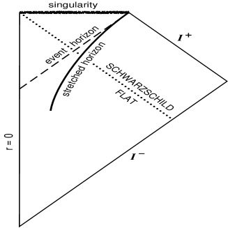
Figure 6: Penrose diagram for a black hole formed by an infalling shell of lightlike matter.

Now consider a nonstatic geometry corresponding to the formation of a large black hole by infalling matter. The simplest case to study involves a thin spherical shell of massless matter [55]. The geometry is constructed by matching flat spacetime and a massive Schwarzschild solution across a radial null surface as shown in Figure 6. The solution for a more general distribution of incoming null matter can approximated by a sequence of shells with the appropriate matching conditions satisfied at each shell.

A stretched horizon can be defined as a timelike surface just outside the event horizon. There are a number of ways to achieve this, but a simple method is as follows [35]. At a point on the global event horizon construct the past directed radial null ray which does not lie in the horizon itself. The stretched horizon is defined to intersect this ray at a point where the area of the transverse two-sphere has increased by an amount of order a Planck unit relative to the area where the ray intersects the event horizon. A feature of the collapse geometry as compared with a static black hole is that both the event horizon and the stretched horizon extend into the flat spacetime region inside the infalling matter shell. With our definition the stretched horizon begins at the same finite value of advanced time as the event horizon itself (see Figure 6). At this point the area of the stretched horizon is only one Planck unit and it is not very meaningful to extend its definition to earlier times.

The stretched horizon defined in this way has the important property that the proper acceleration is of order one in Planck units everywhere on it, independent of time, even including the point where it crosses the incoming matter shell. As a result the stretched horizon can again be viewed as a hot boundary with a Planckian temperature.

6 Gedanken Experiments Involving Black Holes

In this section we will illustrate the concept of black hole complementarity by considering some gedanken experiments where one might expect contradictions to arise. The main conclusion will be that apparent contradictions can always be traced to unsubstantiated assumptions about physics at or above the Planck scale. This observation does not resolve the information problem but it challenges the commonly held view that the paradox can be posed without any reference to the underlying short-distance physics.

6.1 A Test of Information Duplication

It is important to determine whether black hole complementarity leads to observable duplication of information. The results of measurements performed inside a black hole are not available to outside observers. Consider therefore a gedanken experiment [56] where an observer first learns the result of a measurement made on the outgoing Hawking radiation and then enters the black hole in order to receive a signal from some system that previously fell through the event horizon. The system could for example be a measuring apparatus $A$ which carries one member of a pair of ‘spins’ $a$ and $b$, that have been prepared in a singlet state outside the black hole. By ‘spin’ we mean an internal label which is not coupled to a long-range gauge or gravitational field so that it does not lead to classical black hole hair. The apparatus is programmed to measure the spin $a$ once it is inside the event horizon and transmit the result. The other member of the spin pair $b$ remains outside and a team of observers, hovering at a safe distance outside, makes measurements on the Hawking radiation. Since all infalling information is assumed to be radiated out the observers will eventually be able to determine the state of the spin that was carried inside. Armed with this information one of the observers $O$ now enters the black hole in order to receive the signal from the apparatus.

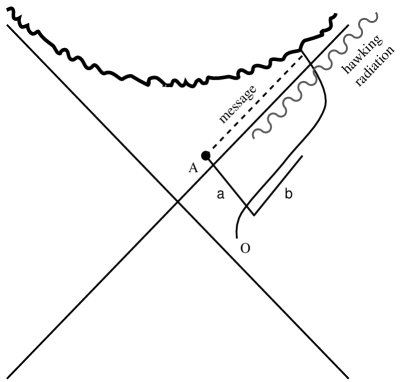
Figure 7: A gedanken experiment designed to test duplication of quantum information.

It would appear that our observer has managed to learn the results of two separate measurements of the same spin. This violates the principles of quantum mechanics as can be seen as follows. The spin $a$ that is carried into the black hole is anti-aligned with $b$, the one that remains outside. From the point of view of an external observer a measurement of the ‘spin in the Hawking radiation’ $h$ amounts to a measurement of the original spin $a$, and therefore $h$ must also be anti-aligned with $b$. The observer $O$ would learn that measurements of $a$ and $h$ along any axis would always give the same result, while for any quantum state of two spins such measurements can at most agree along a single axis.

It turns out to be impossible to carry out this experiment employing only low energy physics [57]. The outside observers have to carry out correlation measurements on the outgoing Hawking radiation for a very long time before they can hope to recover the information about the spin that is sent into the black hole. This time was estimated in [56] to be a finite fraction of the black hole lifetime, i.e. of order $M^{3}$. The estimate is based on some general results found by Page [58] on the entanglement entropy of subsystems in statistical mechanics. Based on this, let us take as given that the distant observers have to conduct experiments for a period of order $M^{3}$ before any information can be recovered. During this time the mass of an evaporating black hole significantly decreases but we shall ignore this and make use of a static Schwarzschild geometry. It will become apparent that the effect of evaporation is to strengthen the conclusion from the static case.

Since we want to discuss measurements made inside a black hole it is convenient to use Kruskal coordinates $U$ and $V$ which extend past the event horizon and are defined in terms of Schwarzschild coordinates through

$$\!\!\begin{array}[]{l}-UV=16M^{2}({r\over 2M}-1)\exp{({r\over 2M}-1)}\,,\\ {}\\ -U/V=\exp{({t\over 2M})}\,.\end{array}$$ (96)

The Schwarzschild line element (94) becomes

$$ds^{2}=-{2M\over r}\exp{(-{r\over 2M}{+}1)}dUdV+r^{2}d\Omega^{2}.$$ (97)

The future event horizon is at $U=0$ and the singularity is at $UV=1$. The geometry is shown in Figure 7. If we choose the origin of our time coordinate so that the apparatus passes through the event horizon at $V=1$ then the observer $O$, who waits outside for a period of order $M^{3}$ as measured by Schwarzschild time, will enter at $V\sim\exp{(M^{2})}$. If the message is to be received before $O$ hits the singularity it must be sent before the apparatus reaches $U\sim\exp{(-M^{2})}$. Near $V=1$ this corresponds to an extremely short proper time $\tau\sim M^{2}\exp{(-M^{2})}$, and the uncertainty principle then dictates that the message must be encoded into radiation with super-Planckian frequency $\omega\sim M^{-2}\exp{(M^{2})}$. It is clear that the apparatus cannot communicate the result of its measurement to the observer $O$ employing only low-energy physics. The evaporation of the black hole only makes the time available for $O$ to receive the message shorter.

It is a generic feature of gedanken experiments of this type that short distance physics enters into their analysis in an essential way and any apparent contradiction with black hole complementarity can be traced to unwarranted assumptions about physics beyond the Planck scale.

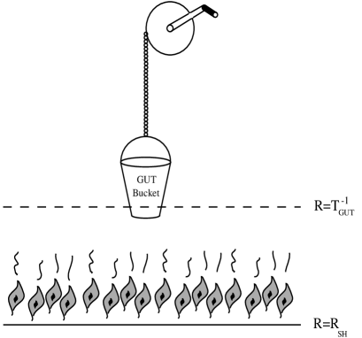
Figure 8: A gedanken experiment to test baryon number non-conservation near the stretched horizon. $R$ denotes the proper distance from the event horizon.

6.2 Thermal Effects Near the Stretched Horizon

Another class of experiments involves attempts by external observers to detect whether quantum information is stored at the stretched horizon. Their analysis also requires short-distance physics even for a large black hole [56]. We will not discuss those experiments here but a closely related one instead, which illustrates how knowledge of high-energy effects can help resolve an apparent contradiction between observations in different reference frames. The effect in question is the violation of baryon number in the process of black hole formation and evaporation. The high-energy physics involved is at the GUT scale rather than the Planck scale.

One of the thermal effects we expect to take place in the reference frame of asymptotic observers is baryon number violation. This effect will become noticeable when matter passes within a proper distance of order $M_{\rm GUT}^{-1}$ of the event horizon and will not be hidden inside the black hole. In order to verify this, a technologically advanced observer could prepare a sealed ‘bucket’ with walls that transmit heat but not baryon number. The bucket is then slowly lowered towards the black hole and retrieved after its bottom edge comes within a proper distance of $M_{\rm GUT}^{-1}$ from the event horizon, as indicated in Figure 8. The baryon number in the bucket is measured before and after lowering and according to the asymptotic observer thermal effects induce a change. The effect can be attributed to the intense acceleration, which the bucket undergoes to avoid falling into the black hole.

Now imagine that the bucket is dropped into the black hole. The asymptotic observer would again say that the bucket encounters a thermal bath but an inertial observer traveling with the bucket in free fall would disagree. This does not lead to any contradiction unless the infalling observer manages to count the baryons in the bucket and transmit the result to the outside observer before the bucket passes through the event horizon. The bucket will, however, only spend a time of order $M_{\rm GUT}^{-1}$ in the region of interest, according to the clock in the free fall frame, and the infalling observer must complete the baryon count in that time. This is precisely the timescale of short lived processes which continuously violate baryon number in the bucket rest frame. Such rapid counting of baryons will not yield the same answer as a leisurely measurement at the beginning of the experiment and the contradiction is avoided.

7 The Stretched Horizon in String Theory

If the ideas presented above are correct then it is essential to gain understanding of physics at very short distances in order to fully resolve the issue of information loss. String theory is widely believed to provide a consistent short-distance description of matter and gravity and Susskind [11] has argued that the kinematic behavior of fundamental strings is entirely consistent with the requirements of black hole complementarity. The basis for this claim is that zero-point fluctuations of string modes make the size of a string depend on the time resolution employed [59]. The shorter the time over which the oscillations of a string are averaged the larger is its spatial extent will appear.

7.1 Infalling String Near The Horizon

Consider a string configuration in free fall approaching a black hole event horizon. An observer at rest far away from the black hole measures asymptotic time, but because of the increasing redshift, a unit of asymptotic time corresponds to an ever shorter time interval in the free-fall frame. The distant observer is therefore using a shorter and shorter resolution time to describe the string configuration and, once it passes within a proper distance of order the string scale from the event horizon, the string begins to spread both in the longitudinal and transverse directions. The longitudinal spread is sufficiently rapid to cancel out the longitudinal Lorentz contraction caused by the black hole geometry. Meanwhile, the spread in the transverse directions causes the configuration to cover the entire horizon area in a time which is short compared to the black hole lifetime.

The stretched horizon is thus made out of the strings in the infalling matter which forms the black hole. On the other hand, this spreading effect is not present in the free-fall frame, where there is no redshift to enhance the time resolution, and from the point of view of an infalling observer there is no stretched horizon, in line with the principle of black hole complementarity.

The string spreading effects in which we are interested take place on a short timescale compared to the black hole lifetime [11] and we therefore consider a static classical geometry. Furthermore, the spreading takes place in a thin layer, whose proper thickness is of order the string scale $1/gM_{Pl}$, outside the event horizon and for a macroscopic black hole this region is well approximated by Rindler space. This is apparent if we consider the the Schwarzschild line element, expressed in Kruskal coordinates, as $r\rightarrow 2M$. In this limit the event horizon looks locally like a planar surface and (97) reduces to

$$ds^{2}=-dU\,dV+d{X^{\perp}}^{2}\,.$$ (98)

The null coordinates $U,V$ extend into the black hole interior and are appropriate for an observer passing through the horizon in free fall. They are related to the null coordinates $u,v$ of an asymptotic observer through,

$${U\over 4M}=-e^{-u/4M}\,,\qquad{V\over 4M}=e^{v/4M}\,.$$ (99)

The usual description of Rindler space is obtained by rescaling all the coordinates to absorb the factors of $4M$, but here we will keep these factors explicit.

Rindler space is isomorphic to a slice of flat Minkowski space, where we can discuss free string propagation in light-cone gauge. Consider an infalling string described by transverse coordinates $X^{i}(\sigma,\tau)$, with $i=1,2$, and some internal degrees of freedom depending on the string model in question. In the free-fall frame the light-cone gauge condition is $\tau=U/4M$. The internal degrees of freedom decouple from the transverse coordinates which satisfy a free wave equation,

$$\bigl{[}\partial^{2}_{\tau}-\partial^{2}_{\sigma}\bigr{]}X^{i}(\sigma,\tau)=0\,.$$ (100)

The solution can be expressed by the usual sum over modes of oscillation, but, unless the infinite sum is cut off in some way, this leads to ill-defined expressions for quantities such as the average transverse area occupied by the string in the quantum theory [59]. Introducing a cutoff on the mode expansion corresponds physically to employing finite time resolution so that mode oscillations above a given frequency average out. The string wave-function extends over a transverse area which grows logarithmically with better resolution time while the average length of string projected onto the transverse directions grows linearly. This means that the string density will increase at the center of the distribution, and eventually we can no longer neglect the effect of string interactions there.

Now we want to consider the string evolution in the reference frame of a distant fiducial observer, whose retarded time, $t=u$, is related to the worldsheet parameter time through

$${\tau}=-e^{-{t/4M}}\>.$$ (101)

As asymptotic time goes on, a fixed resolution in $t$ thus corresponds to an exponentially improving resolution in $\tau$, so that in the reference frame of the distant observer, the string wave-function will spread with time to occupy a transverse area proportional to $t$. By using the constraint equations of light-cone string theory one can show that the string also spreads in the longitudinal direction and that the longitudinal spreading is rapid enough to balance the Lorentz contraction due to the black hole metric near the event horizon [11].

7.2 Branching Diffusion of String Bits

Since the stringy stretched horizon is formed from the infalling matter itself, it efficiently absorbs the quantum information contained in that matter. The string spreading process also thermalizes the stretched horizon [60]. This is seen as follows. In asymptotic time $t$ the equation of motion (100) of the field $X^{i}\bigl{(}\sigma,\tau(t)\bigr{)}$ becomes

$$\bigl{[}\partial_{t}^{2}+\frac{1}{4M}\partial_{t}-\bigl{(}\frac{e^{-t/4M}}{4M}\bigr{)}^{2}\partial_{\sigma}^{2}\bigr{]}X^{i}(\sigma,t)=0\,.$$ (102)

Now split both the field $X^{i}$ and its conjugate momentum $\partial_{t}X^{i}$ into a slowly varying, classical part and fast varying, quantum part,

$$\!\!\begin{array}[]{l}X^{i}(\sigma,t)=x^{i}(\sigma,t)+x_{f}^{i}(\sigma,t)\,,\\ {}\\ \partial_{t}X^{i}(\sigma,t)=v^{i}(\sigma,t)+v_{f}^{i}(\sigma,t)\,.\end{array}$$ (103)

The quantum field $x_{f}^{i}$ can be expressed as a sum over modes in the $(\tau,\sigma)$ frame, provided the frequency cutoff, which separates the fast modes from the slow ones, is chosen to reflect the exponentially improving resolution in $\tau$,

$$x_{f}^{i}(\sigma,t)=\sqrt{{\alpha^{\prime}\over 2}}\sum_{n=1}^{\infty}W(n+\frac{\epsilon}{\tau})\bigl{[}\frac{c_{n}^{i}}{\sqrt{n}}e^{-in(\tau{+}\sigma)}$$ (104)

$$\qquad\>+\frac{\tilde{c}_{n}^{i}}{\sqrt{n}}e^{-in(\tau{-}\sigma)}+H.c.\bigr{]}\,,$$

where $\epsilon$ is some constant. The expansion for $v_{f}^{i}$ is similar. For a filter function one could use $W(n+\frac{\epsilon}{\tau})=\theta(n+\frac{\epsilon}{\tau})=\theta(n-\epsilon\,e^{t/4M})$. Then an asymptotic observer would indeed include only modes of exponentially higher frequency in the definition of the quantum part of the field. In actual calculations it is better to use a filter where the step of the theta function is smeared a little, in order to avoid unphysical effects associated with a sharp edge cutoff in two dimensions.

The long-wavelength field $x^{i}$ will evolve nontrivially in asymptotic time due to the continual feeding in of modes from the quantum fields. This evolution is described by a simple Langevin equation [60]

$$\partial_{t}x^{i}=\eta^{i}\,,$$ (105)

with noise correlator

$$\langle\eta^{i}(1)\,\eta^{j}(2)\rangle\simeq\frac{\alpha^{\prime}}{2}\,\frac{\delta^{ij}}{4M}\,\delta(t_{1}{-}t_{2})\,\cos(\frac{\epsilon\Delta\sigma}{\tau})$$ (106)

$$\qquad\qquad\times\exp\bigl{[}-\frac{\beta^{2}}{4}\bigl{(}\frac{\epsilon\Delta\sigma}{\tau}\bigr{)}^{2}\bigr{]}\,.$$

The time-dependence in the correlator assures us that the noise $\eta^{i}$ is white, and the spatial dependence tells us that wee bits of string of parameter length $\Delta\sigma\simeq|\tau|/(\beta\epsilon)$ evolve independently with time.

The Langevin equation in (105) describes a branching diffusion process which thermalizes the string configuration. At any given point of the string the value of the slowly-varying field $x^{i}(\sigma,t)$ experiences a Brownian motion which is essentially unaffected by anything lying outside the correlation length $\Delta\sigma\approx|\tau|/\beta\epsilon$. This resembles the independence of the scalar field evolution in different Hubble domains in the case of chaotic inflation [63]. The correlation length decreases exponentially with asymptotic time and therefore the number of such independent bits of the string increases exponentially:

$$N\sim\frac{2\pi\beta\epsilon}{|\tau|}=2\pi\beta\epsilon\,\exp(t/4M)\,.$$ (107)

The diffusion of a given bit of string is governed by the Fokker-Planck equation,

$$\partial_{t}P(x^{i},t)=\frac{\varsigma^{2}}{2}\delta^{ij}\partial_{i}\partial_{j}P(x^{i},t)\,.$$ (108)

where $P(x^{i},t)$ is the normalized probability of finding that bit at $(x^{i},t)$. On the stretched horizon of a finite-mass black hole, $P\rightarrow constant$ at late times.

The coefficient of diffusion can be read off the correlator of the noise, $\varsigma^{2}=\frac{\alpha^{\prime}}{8M}$, and the mean square transverse position is given by

$$\langle x^{i}x^{i}\rangle=2\varsigma^{2}t=\frac{\alpha^{\prime}}{4M}\,t\,.$$ (109)

This is the transverse spread, linear in asymptotic time, pointed out by Susskind [11]. The string will spread to cover the area of the black hole horizon in a time

$$t_{S}\sim g^{2}M^{3}\,,$$ (110)

where $M$ and $t$ are measured in Planck units and $g$ is the string coupling strength. This is a short time compared to the black hole lifetime if the string is weakly coupled.

Another important timescale is that on which the volume density of string at the center of the distribution becomes $O(1/g^{2})$ in string units. At this point string interactions can no longer be ignored and the above calculations, which are all at the level of free string theory, no longer apply. The proper thickness of the stretched horizon remains of order one in string units while the average area occupied increases linearly with time. At the same time the average number of string bits grows exponentially so the time $t_{I}$ at which string interactions become important at the center of the distribution of string bits is:

$$t_{I}\sim M\log{(1/g^{2})}\,.$$ (111)

For a macroscopic black hole this timescale is very much shorter than the spreading time $t_{S}$. An attractive possibility, pointed out in [11], is that string interactions prevent the volume density from exceeding $O(1/g^{2})$ and that the central density will level off at that value. This volume density corresponds to an $O(1)$ area density of string bits on the stretched horizon measured in Planck units, the value suggested by the Bekenstein-Hawking entropy. If string interactions prevent the density from increasing beyond $O(1/g^{2})$, this will produce an outward pressure that spreads the string bits much more rapidly than the diffusion of the free theory [64].

We have presented evidence in support of the view that a stretched horizon made out of strings has a key role to play in resolving the black hole information paradox. For technical reasons the discussion was limited to strings approaching the horizon of a classical black hole in the limit of infinite mass. We cannot at present establish, although we find it very plausible, that the stringy stretched horizon re-emits the original information encrypted in apparently thermal Hawking radiation. Another important issue to address concerns the underlying causal properties of string theory which allow the spread of information across the stretched horizon [65].

I wish to thank the organizers for the opportunity to lecture at the Spring School and for their hospitality at the ICTP Trieste. I have benefited from discussions on black holes with many friends and colleagues and I want especially to thank my collaborators: A. Mezhlumian, A. Peet, J. Russo, A. Strominger, L. Susskind and J. Uglum. I also thank S. Giddings, A. Strominger, and J. Uglum for helpful comments on the manuscript.

References

- [1] S.W. Hawking, Commun. Math. Phys. 43 (1975) 199.
- [2] S.W. Hawking, Phys. Rev. D14 (1976) 2460.
- [3] See e.g. S.W. Hawking and G.F.R. Ellis, The Large Scale Structure of Spacetime, Cambridge University Press, Cambridge, 1973.
- [4] S.W. Hawking, Commun. Math. Phys. 87 (1982) 395.
- [5] J. Ellis, J. Hagelin, D.V. Nanopoulos, and M. Srednicki, Nucl. Phys. B241 (1984) 381.
- [6] T. Banks, L. Susskind, and M. Peskin, Nucl. Phys. B244 (1984) 125.
- [7] D. Gross, Nucl. Phys. B236 (1984) 349.
- [8] A. Strominger, Unitary Rules for Black Hole Evaporation, hep-th 9410187, UCSBTH-94-34, October 1994.
- [9] D. Page, Phys. Rev. Lett. 44 (1980) 301.
- [10] G. ‘t Hooft, Nucl. Phys. B335 (1990) 138; Phys. Scr. T36 (1991) 247, and references therein.
- [11] L. Susskind, Phys. Rev. Lett. 71 (1993) 2367; Phys. Rev. D49 (1994) 6606.
- [12] Y. Aharonov, A. Casher, and S. Nussinov, Phys. Lett. B191 (1987) 51.
- [13] T. Banks and M. O’Loughlin, Phys. Rev. D47 (1993) 540; T. Banks, M. O’Loughlin, and A. Strominger, Phys. Rev. D47 (1993) 4476; A. Strominger and S. Trivedi, Phys. Rev. D48 (1993) 5778; S.B. Giddings, Phys. Rev. D48 (1994) 947; ibid. 4078.
- [14] J. Polchinski and A. Strominger, A Possible Resolution of the Black Hole Information Puzzle, UCSBTH-94-20, hep-th 9407008, July 1994.
- [15] C.G. Callan, S.B. Giddings, J.A. Harvey, and A. Strominger, Phys. Rev. D45 (1992) 1005.
- [16] J.A. Harvey and A. Strominger, in the Proceedings of the TASI Summer School, June 3-28, 1992, Boulder, Colorado, (World Scientific, 1993).
- [17] S.B. Giddings, in the Proceedings of the International Workshop on Theoretical Physics, 6th Session, June 21-28, 1992, Erice, Italy, (World Scientific, 1993).
- [18] S.B. Giddings and A. Strominger, Phys. Rev. D46 (1992) 627.
- [19] T. Banks, A. Dabholkar, M.R. Douglas, and M. O’Loughlin, Phys. Rev. D45 (1992) 3607.
- [20] G. Horowitz, in String Theory and Quantum Gravity ’92, J.A. Harvey et al. eds., World Scientific (1993).
- [21] E. Witten, Phys. Rev. D44 (1991) 314.
- [22] J.G. Russo, L. Susskind, and L. Thorlacius, Phys. Lett. B292 (1992) 13.
- [23] S.M. Christensen and S.A. Fulling, Phys. Rev. D15 (1977) 2088.
- [24] S.B. Giddings and W.M. Nelson, Phys. Rev. D46 (1992) 2486.
- [25] For a recent discussion of this issue see T. Jacobson, Phys. Rev. D48 (1993) 728.
- [26] B. Birnir, S.B. Giddings, J.A. Harvey, and A. Strominger, Phys. Rev. D46 (1992) 638.
- [27] L. Susskind and L. Thorlacius, Nucl. Phys. B382 (1992) 123.
- [28] S.W. Hawking, Phys. Rev. Lett. 69 (1992) 406.
- [29] D.A. Lowe, Phys. Rev. D47 (1993) 2446; T. Piran and A. Strominger, Phys. Rev D48 (1993) 4729.
- [30] A. Bilal and C.G. Callan, Nucl. Phys. B394 (1993) 73.
- [31] S.P. de Alwis, Phys. Lett. B289 (1992) 278; B300 (1993) 330; Phys. Rev. D46 (1992) 5429.
- [32] J.G. Russo, L. Susskind, and L. Thorlacius, Phys. Rev. D46 (1992) 3444; Phys. Rev. D47 (1993) 533.
- [33] A. Strominger, Phys. Rev. D48 (1993) 5769.
- [34] A. Strominger and S. Trivedi, unpublished.
- [35] L. Susskind, L. Thorlacius, and J. Uglum, Phys. Rev. D48 (1993) 3743.
- [36] T.D. Chung and H. Verlinde, Nucl. Phys. B418 (1994) 305.
- [37] S.R. Das and S. Mukherji, Phys. Rev. D50 (1994) 930.
- [38] A. Strominger and L. Thorlacius, Phys. Rev. 50 (1994) 5177.
- [39] N. Seiberg, S. Shenker, L. Susskind, L. Thorlacius, and J. Tuttle, unpublished (1992).
- [40] See e.g. N. Birrel and P. Davies Quantum Fields in Curved Space (Cambridge University Press, 1982) and references therein; R. Carlitz and S. Willey, Phys. Rev. D36 (1987) 2327, 2336; F. Wilczek, IAS preprint HEP-93/12, hep-th 9302096.
- [41] A. Anderson and B. DeWitt, Found. Phys. 16 (1986) 91.
- [42] J.G. Russo and A.A. Tseytlin, Nucl. Phys. B382 (1992) 259.
- [43] S.B. Giddings and A. Strominger, Phys. Rev. D47 (1993) 2754.
- [44] T. Burwick and A. Chamseddine, Nucl. Phys. B384 (1992) 411.
- [45] J. Polchinski, Nucl. Phys. B324 (1989) 123; T. Banks, Physicalia Magazine, vol 12, Special Issue in Honor of the 60th Birthday of R.Brout, Gent (1990); S.R. Das, S. Naik, and S.R. Wadia, Mod. Phys. Lett. A4 (1990) 1033; S.R. Das, A. Dhar, and S.R. Wadia, Mod. Phys. Lett. A5 (1990) 799; T. Banks and J. Lykken, Nucl. Phys. B331 (1990) 173; A.A. Tseytlin, Int. Jour. Mod. Phys. A5 (1990) 1833.
- [46] A. Strominger, Phys. Rev. D46 (1992) 4396.
- [47] E. Verlinde and H. Verlinde, Nucl. Phys. B406 (1993) 43; K. Schoutens, E. Verlinde, and H. Verlinde, Phys. Rev. D48 (1993) 2690.
- [48] J.L. Cardy, Nucl. Phys. 240 (1984), 514.
- [49] D. Lowe, J. Polchinski, A. Strominger, and L. Thorlacius, unpublished (1994).
- [50] O. Lechtenfeld and C. Nappi, Phys. Lett. B288 (1992) 72; V. Frolov, Phys. Rev. D46 (1992) 5383.
- [51] T. Banks and M. O’Loughlin, Phys. Rev. D48 (1993) 698; D. Lowe and M. O’Loughlin, Phys. Rev. D48 (1993) 3735; A. Strominger and S. Trivedi, Phys. Rev. D48 (1993) 5778.
- [52] M. Maggiore, Phys. Rev. D49 (1994) 2918; Phys. Lett. B333 (1994) 39.
- [53] S.D. Mathur, Black Holes Entropy and the Semiclassical Approximation, January 1994, hep-th 9404135; E. Keski-Vakkuri, G. Lifschytz, S.D. Mathur, and M. Ortiz, Breakdown of the Semiclassical Approximation at the Black Hole Horizon, MIT-CTP-2341, hep-th 9408039, July 1994;
- [54] K.S. Thorne, R.H. Price, and D.A. MacDonald, Black Holes: The Membrane Paradigm, Yale University Press, New Haven, CT, 1986, and references therein.
- [55] W.G. Unruh, Phys. Rev. D14 (1976) 870. Y. Choquet-Bruhat, Ann. Inst. Henri Poincaré 8 (1968) 327;
- [56] L. Susskind and L. Thorlacius, Phys. Rev. D49 (1994) 966.
- [57] J. Preskill, private communication (1993); H. Verlinde, private communication (1993).
- [58] D. Page, Phys. Rev. Lett. 71 (1993) 1291.
- [59] L. Susskind, Phys. Rev. D1 (1970) 1182; M. Karliner, I. Klebanov, and L. Susskind, Int. J. Mod. Phys. A3 (1988) 1981.
- [60] A. Mezhlumian, A. Peet, and L. Thorlacius, Phys. Rev. D50 (1994) 2725.
- [61] R. Giles and C.B. Thorn, Phys. Rev. D16 (1977) 366; C.B. Thorn, Phys. Rev. D17 (1978) 1073; D19 (1979) 639; Calculating the Rest Tension for a Polymer of String Bits, UFIFT-HEP-94-8, hep-th 9407169, July 1994.
- [62] I. Klebanov and L. Susskind, Nucl. Phys. B309 (1988) 175.
- [63] A.D. Linde and A. Mezhlumian, Phys. Lett. B307 (1993) 25; A.D. Linde, D.A. Linde, and A. Mezhlumian, Phys. Rev. D49 (1994) 1783.
- [64] L. Susskind, The World as a Hologram, SU-ITP-94-33, hep-th 9409089, September 1994.
- [65] E. Martinec, Class. Quant. Grav. 10 (1993) L187; D.A. Lowe, Phys. Lett. B326 (1994) 223; D.A. Lowe, L. Susskind, and J. Uglum, Phys. Lett. B327 (1994) 226.