NSF-ITP-94-96

hep-th/9409168

ABSTRACT: An infinite number of distinct $d=1$ matrix models reproduce the perturbation theory of $d=2$ string theory. Due to constraints of causality, however, we argue that none of the existing constructions gives a consistent nonperturbative definition of the $d=2$ string.

The search for a nonperturbative formulation of string theory remains a key open problem. String theories in two or fewer spacetime dimensions, which are exactly solvable by matrix model methods, have been valuable model systems; for reviews, see ref. [1]. One notable feature of these models is the large-order growth of perturbation theory, more rapid than in field theory and so corresponding to larger nonperturbative effects. This growth was subsequently found to be generic to string theory in higher dimensions[2].

Another notable, and puzzling, feature is a very large non-perturbative ambiguity. There is an infinite-parameter set of distinct $d=1$ matrix models, all of which reproduce the perturbation theory for the $d=2$ string and all of which are consistent quantum theories[3]. This has been interpreted as the existence of an infinite number of non-perturbative parameters analogous to the $\theta$-parameter of QCD.

In fact, we will argue that the situation is quite the opposite—that none of the proposed non-perturbative definitions gives rise to a consistent string theory, and that the problem of finding any consistent non-perturbative formulation of the $d=2$ string remains open. This result is a simple but unexpected consequence of a recent study of spacetime gravity in these models[4].

To review: after diagonalizing and double-scaling, the matrix model becomes a theory of free fermions in an inverted harmonic oscillator potential[5, 6]. In terms of a second-quantized fermion $\psi(x,t)$ with $x$ the rescaled eigenvalue, the Hamiltonian is

$$H=\frac{1}{2}\int_{-\infty}^{\infty}dx\,\Bigl{\{}\partial_{x}\psi^{\dagger}\partial_{x}\psi-x^{2}\psi^{\dagger}\psi\Bigr{\}}\ .$$ (1)

The string tachyon, which is the only propagating degree of freedom in $d=2$, corresponds to the collective motion of the Fermi surface[7]. The static solutions are given by filling the Fermi sea on one side of the barrier, say the left, to an energy $-\overline{\mu}$, below the maximum of the potential. In string perturbation theory, at fixed energy and fixed number of external particles, the other side of the barrier is irrelevant. The asymptotic region $\phi\to-\infty$ of the string Liouville coordinate corresponds to the asymptotic region $x\to-\infty$ of eigenvalue space.

Fermions will tunnel through the potential barrier; this is the anomalously large non-perturbative effect mentioned above. To define the theory non-perturbatively we must make a prescription for the state on the other side of the barrier. One class of theories (type I in the terminology of ref. [3]) eliminates the second asymptotic region by modifying the potential. For example, a sharp infinite barrier, $V(x)=\infty$ for $x>A$, leaves the perturbation theory unaffected for any $A\geq 0$. So does any other modification such that $V(x)$ is $-\frac{1}{2}x^{2}$ for $x<0$ and rises to infinity as $x\to\infty$. All such modifications give the same perturbation theory, and all produce a manifestly unitary quantum theory within the Hilbert space of incoming and outgoing fermions in the left asymptotic region (or the bosonized equivalent). Nevertheless, we will argue that no matrix model of type I corresponds to a consistent string theory. An alternate approach to defining the theory is to leave the potential unmodified and work within the larger space of states of two asymptotic regions (type II), for example by filling the right Fermi sea to the same level $-\overline{\mu}$. We will argue that at least the naive implementation of this idea is inconsistent.

Since the type I matrix models are certainly consistent quantum theories in their own right, why do we assert that they correspond to inconsistent string theories? The additional consistency condition we impose is causality. For example, the non-perturbative dynamics must conserve the gravitational mass, which can be measured by scattering experiments arbitrarily far into the asymptotic region. That this is a nontrivial condition follows from the rather convoluted way that gravitational physics is encoded in the matrix model[4]. In fact, the $d=2$ string must satisfy an infinite set of such causality conditions.

Rather than gravitational scattering, we will focus on the simplest process that leads to a causality condition, namely $2\to 1$ bulk tachyon scattering. That is, a pair of incoming tachyons have an amplitude to scatter into an outgoing tachyon before reaching the Liouville wall. This amplitude is nonzero because the operator product of three tachyon vertex operators contains the identity, but does not occur in the matrix model because a small free-fermi pulse will always travel to the turning point $x=-\sqrt{2\overline{\mu}}$ before reflecting. The difference arises because of the nonlocal relation between the string tachyon and the collective field of the matrix model[8, 4].

Let us briefly review how this comes about. Comparison of the matrix model and string S-matrices shows that the respective tachyon fields are related in the asymptotic region by the so-called ‘leg pole’ factor

$${\cal S}(\phi,t)\ =\ \biggl{(}\frac{\pi}{2}\biggr{)}^{-\partial_{\phi}/4}\frac{\Gamma(-\partial_{\phi})}{\Gamma(\partial_{\phi})}\overline{\cal S}(\phi,t),$$ (2)

where the bar identifies the matrix model field. The string tachyon $\cal S$ is a function of $\phi$ and $t$, while the matrix model tachyon $\overline{\cal S}$ is defined as a function of $q$ (logarithm of the eigenvalue, defined below) and $t$. Eq. (2) relates the $\phi$-dependence of $\cal S$ to the $q$-dependence of $\overline{\cal S}$. This transformation is nonlocal, and gives rise to bulk scattering as shown in figure 1.

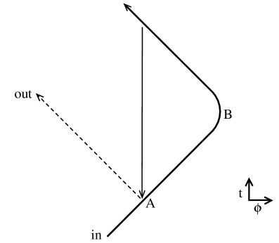
Figure 1: Two tachyons in an incoming pulse can backscatter into one (dashed line) at a given point A. In the matrix model all tachyons pass through the turning region B. The nonlocal renormalization (2), vertical arrow, produces the outgoing wave.

To analyze this it is useful to introduce the conserved charges[9]

$$v_{mn}=e^{(n-m)t}\int_{F-F_{0}}\frac{dp\,dx}{2\pi}\,(-x-p)^{m}(-x+p)^{n},$$ (3)

with Poisson bracket algebra

$$\{v_{mn},v_{m^{\prime}n^{\prime}}\}=2(m^{\prime}n-n^{\prime}m)v_{m+m^{\prime}-1,n+n^{\prime}-1}.$$ (4)

The phase space integral (3) runs over the interior $F$ of the Fermi sea, minus the interior $F_{0}$ of the static sea, $x<-\sqrt{p^{2}+2\overline{\mu}}$. These are conserved because

$$(-x-p)e^{-t},\qquad(-x+p)e^{t}$$ (5)

are constants of the motion in the inverted harmonic potential. For perturbations which are not too large, the Fermi sea can be described in terms of its upper and lower surfaces $p_{\pm}(x,t)$. Asymptotically, these move with velocity 1 in the coordinate $q=-\ln(-x)$,

$$p_{\pm}(x,t)\ \sim\ \mp x\pm\frac{1}{x}\epsilon_{\pm}(t\mp q),$$ (6)

where the upper and lower signs refer respectively to the incoming and outgoing waves. The incoming and outgoing parts of the canonically normalized matrix model scalar are related to the perturbation of the Fermi sea by

$$\partial_{q}\overline{\cal S}_{\pm}(t\mp q)=-\frac{1}{2\sqrt{\pi}}\Bigl{\{}\epsilon_{\pm}(t\mp q)-\overline{\mu}\Bigr{\}}.$$ (7)

Evaluating the charge (3) in the limits $t\to\mp\infty$ gives a relation between the incoming and outgoing waves,

$$v_{mn} = \frac{2^{n}}{2\pi(m+1)}\int_{-\infty}^{\infty}dt\,e^{(n-m)(t-q)}\Bigl{\{}(\epsilon_{+}(t-q))^{m+1}-\overline{\mu}^{m+1}\Bigr{\}}$$ (8)

$$= \frac{2^{m}}{2\pi(n+1)}\int_{-\infty}^{\infty}dt\,e^{(n-m)(t+q)}\Bigl{\{}(\epsilon_{-}(t+q))^{n+1}-\overline{\mu}^{n+1}\Bigr{\}}.$$

The $2\to 1$ bulk scattering is now derived as follows. To resolve the bulk scattering we use narrow wave packets as in ref. [4], so the leading behavior as $t+\phi\to-\infty$ comes from the first pole in the renormalization (2), at $\partial_{\phi}=1$. Near this point the renormalization factor is $(\pi/2)^{-1/4}(\partial_{\phi}-1)^{-1}$, giving

$$\lim_{t+\phi\to-\infty}{\cal S}_{-}(t+\phi) = -2^{1/4}\pi^{-1/4}e^{t}\int_{t}^{\infty}dt^{\prime}\,e^{-t^{\prime}}\overline{\cal S}_{-}(t^{\prime}+\phi)$$ (9)

$$= -2^{1/4}\pi^{-1/4}e^{t}\int_{-\infty}^{\infty}dt^{\prime}\,e^{-t^{\prime}}\overline{\cal S}_{-}(t^{\prime}+\phi)$$

$$= 2^{-3/4}\pi^{1/4}e^{t+\phi}v_{10}.$$

In the second line we have used the narrowness of the wavepacket to extend the range of integration, and in the third we have noted that the result is simply proportional to the conserved charge $v_{10}$. Now expressing this in terms of the incoming field gives

$$\lim_{t+\phi\to-\infty}{\cal S}_{-}(t+\phi) = 2^{-3/4}\pi^{1/4}e^{t+\phi}\int_{\infty}^{\infty}dt^{\prime}\,e^{-t^{\prime}+\phi}\Bigl{\{}(\partial_{t}\overline{\cal S}_{+}(t-\phi))^{2}+\overline{\mu}\partial_{t}\overline{\cal S}_{+}(t-\phi)/\sqrt{\pi}\Bigr{\}}$$ (10)

$$= 2^{-1/2}e^{t+\phi}\int_{\infty}^{\infty}dt^{\prime}\,e^{-t^{\prime}+\phi}({\cal S}_{+}(t^{\prime}-\phi))^{2}\ +\ O(\overline{\mu})\ .$$

In the second line we have carried out the renormalization (2) in reverse, leading to a simple result after integration by parts. The $O(\overline{\mu})$ term is from $1\to 1$ scattering on the tachyon background.

The result (10) is the same as in ref. [4], but the derivation is actually more general. Ref. [4] used a weak-field expansion, in powers of ${\cal S}$. From the definitions (6) and (7) the weak-field expansion parameter is $\partial_{\phi}{\cal S}_{+}/x^{2}$. There is a second expansion parameter, $1/\overline{\mu}^{2}$, governing the string loop expansion; for convenience we assume this to be small and focus on classical scattering. At large $x$, far in the asymptotic region, $\partial_{\phi}{\cal S}_{+}/x^{2}$ is always small, but the condition that a pulse remain small throughout the scattering is $\partial_{\phi}{\cal S}_{+}\ll\overline{\mu}$ since the turning radius is $O(\overline{\mu}^{1/2})$. Ref. [4] required the latter inequality to hold; the derivation above does not, because a conservation law has been used to relate the incoming and outgoing waves.

This point is important, and a bit confusing, so let us expand on it. The bulk scattering process occurs in asymptotic region where nonlinearities are always small, and so is determined entirely by the cubic term in the effective Lagrangian, known from string perturbation theory to be of the form $e^{2\phi}{\cal S}^{3}$. This must be true even for a pulse with $\partial_{\phi}{\cal S}_{+}\sim\overline{\mu}$. For such a pulse the nonlinearities will eventually become large, but this in a region (the turning region of figure 1) in the future of the point where the bulk scattering occurs, and so must be irrelevant. However, the matrix model completely obscures this causal relationship—the ‘information’ in the incoming pulses always propagates through the turning region before being transferred to the outgoing wave by the nonlocal renormalization. The nonlinearity, even if strong, conserves $v_{mn}$, so the correct amplitude is obtained just the same.

That is, all is well provided the pulse remains below the maximum of the potential, which is to say in the region $x<-|p|$ or $\partial_{q}\overline{\cal S}_{+}<\overline{\mu}/2\sqrt{\pi}$. A pulse which exceeds this, shown in figure 2a, will propagate to positive $x$ and, in the type I theories, feel the modification of the potential.

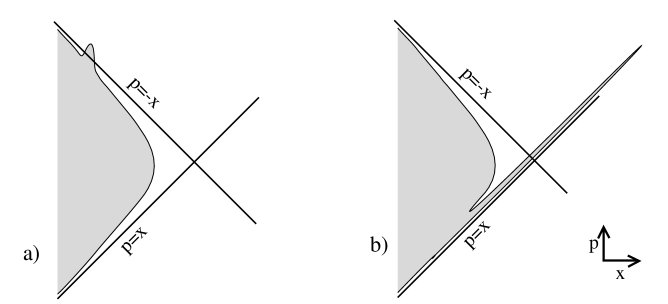
Figure 2: a) Incoming pulse in phase-space plane, extending above the line $p=-x$. Filled states are shaded. b) Later form of the pulse, with part propagating to $x=\infty$.

Consider for example an infinite wall at $A=0$: a fermion reaching the phase space point $(x,p)=(0,p)$ will jump discontinuously to $(0,-p)$. The quantities (5) change discontinuously and so the $v_{mn}$ are not conserved. The bulk scattering amplitude is then not in agreement with string perturbation theory. This is unacceptable, because the bulk scattering occurs in a region where both the string and the weak-field expansion parameters are small, while the strong nonlinearities occur only in the causal future. Moreover this is true for any theory of type I: the quantity $(-x-p)e^{t}$ is negative for incoming fermions above the $p=-x$ line, but is positive for all outgoing fermions.

The scattering process used in ref. [4] to measure the gravitational mass similarly depends upon conservation of $v_{20}$. As it happens, there is one theory of type I which conserves $v_{20}$ and so the gravitational mass, but not $v_{10}$. This is just the theory with infinite barrier at $x=0$, because the sign jump in $(0,p)\to(0,-p)$ cancels when $m+n$ is even. However, the causality violation in $2\to 1$ scattering is still unacceptable.

Other bulk processes require conservation of $v_{m0}$ for all positive integer $m$. It is not clear whether a similar causality argument can be applied to the $v_{mn}$ for $m$ and $n$ nonzero, but there is another way to see that these must be conserved, and therefore that the type I theories are not consistent as string theories. The $v_{mn}$ for $m,n\neq 0$ are just the unbroken symmetries of string field theory discussed in ref. [11], with $v_{s+n,s-n}\ \propto\ A_{s,n}$, and so should be conserved even nonperturbatively.

Even though we are discussing classical scattering this condition is nonperturbative in the $1/\overline{\mu}$ expansion, since the condition for a large pulse is $\overline{\mu}<2\sqrt{\pi}\partial_{q}\overline{\cal S}_{+}.$ That is, the number of incoming tachyons is of order $(1/\overline{\mu})^{-2}$.

The other natural nonperturbative definition of the theory, type II, leaves the potential unmodified. Filling the Fermi sea to the same level $-\overline{\mu}$ on both sides gives a stable state, and the matrix model is a unitary theory with two asymptotic weak coupling regions. But even though the $v_{mn}$ are conserved this is not a consistent string theory, at least with the straightforward interpretation that each asymptotic region of the matrix model corresponds to an asymptotic region of spacetime. The point is that a part of the incoming fermion pulse travels over the barrier, so that the relation (8) between $v_{mn}$ and the left outgoing wave $\epsilon_{-}$ no longer holds and the correct bulk scattering and gravitational mass are no longer obtained.

To summarize, both the type II theory as defined above and the infinite class of type I theories have been previously assumed to define consistent nonperturbative string theories. We have argued that in fact none of these are consistent, and it stands as a challenge to find any consistent nonperturbative definition of the $d=2$ string theory. If one is to make sense of the type II case, it is evidently necessary to identify the asymptotic region of the string theory with some combination of the two asymptotic regions of the matrix model. If one is to make sense of the type I case, the mapping (2) between the matrix model and string Hilbert spaces must be modified. This modification will have to be rather complicated—the simple linear relation (2) appears to be exact as long as the pulses stay below the threshold, while past this point the mapping must change abruptly.

The nonperturbative formulation of string theory is likely to involve unexpected new ideas. The matrix model is one of the few clues available, and so it is important to resolve the issue raised here and construct the exact theory. We believe the correct formulation will not involve modification of the potential, but will require a more subtle mapping between the matrix model and string Hilbert spaces; this is under active investigation.

One of the obstacles to progress in matrix models has been that the number of consistent models—the number of modifications and generalizations that one might try—is much larger than the number of consistent string theories. The causality condition we have introduced is therefore a useful tool in applying matrix models to critical string theory. For example, we have used it in ref. [4] to argue that the proposed matrix model black hole of ref. [12] gives the wrong bulk scattering at long distance (this point is also made in refs. [13] and [14]). As an aside, it seems very likely that pulses which pass over the barrier as in figure 2 are related to black hole formation, so the resolution of the problem we have presented is also likely to lead to progress in this area.

The matrix model might have been interpreted to give evidence for the existence of a large number of nonperturbative parameters in string theory. This would be unsatisfactory for the ultimate predictive power of the theory, and rather surprising as well since all parameters in string theory are believed to be associated with background fields. Our result is thus further evidence for the uniqueness of string theory.

References

- [1] P. Ginsparg and G. Moore, in Recent Directions in Particle Theory, Proceedings of the 1992 TASI, ed. J. Harvey and J. Polchinski (World Scientific, Singapore, 1993), hep-th/9304011; I. Klebanov, in String Theory and Quantum Gravity, Proceedings of the Trieste School 1991, eds. J. Harvey et. al. (World Scientific, Singapore, 1992) hep-th/9108019.
- [2] S. Shenker, in Random Surfaces and Quantum Gravity, eds. O. Alvarez, E. Marinari, and P. Windey (Plenum, 1991).
- [3] G. Moore, M. R. Plesser, and S. Ramgoolam, Nucl.Phys. B377, 143 (1992) hep-th/9111035.
- [4] M. Natsuume and J. Polchinski, “Gravitational Scattering in the Matrix Model,” Nucl. Phys. B424, 137 (1994) hep-th/9402156.
- [5] E. Brézin, C. Itzykson, G. Parisi, and J.-B. Zuber, Comm. Math. Phys. 59, 35 (1978).
- [6] D. J. Gross and N. Miljković, Phys. Lett. B238, 217 (1990); E. Brézin, V. A. Kazakov, and A. B. Zamolodchikov, Nucl. Phys. B333, 673 (1990); P. Ginsparg and J. Zinn-Justin, Phys. Lett. B240, 333 (1990); G. Parisi, Phys. Lett. B238, 209 (1990).
- [7] S. R. Das and A. Jevicki, Mod. Phys. Lett. A5, 1639 (1990); J. Polchinski, Nucl. Phys. B362 (1991) 125; A. M. Sengupta and S. R. Wadia, Int. J. Mod. Phys. A6, 1961 (1991); G. Mandal, A. M. Sengupta, and S. R. Wadia, Mod. Phys. Lett. A6, 1465 (1991).
- [8] A. M. Polyakov, Mod. Phys. Lett. A6, 635 (1991); D. J. Gross and I. R. Klebanov, Nucl. Phys. B359, 3 (1991); P. Di Francesco and D. Kutasov, Phys. Lett. B261, 385 (1991); Nucl. Phys. B375, 119 (1992); N. Sakai and Y. Tanii, Prog. Theor. Phys. Suppl. 110, 117 (1992); Phys. Lett. B276, 41 (1992); G. Minic and Z. Yang, Phys. Lett. B274, 27 (1992); D. Lowe, Mod. Phys. Lett. A7, 2647 (1992).
- [9] J. Avan and A. Jevicki, Phys. Lett. B266, 35 (1991); G. Moore and N. Seiberg, Int. J. Mod. Phys. A7, 2601 (1992); S. R. Das, A. Dhar, G. Mandal, and S. R. Wadia, Int. J. Mod. Phys. A7, 5165 (1992); D. Minic, J. Polchinski, and Z. Yang, Nucl. Phys. B369, 324 (1992).
- [10] G. Moore and R. Plesser, Phys. Rev. D46, 1730 (1992) hep-th/9203060.
- [11] E. Witten, Nucl. Phys. B373, 187 (1992); E. Witten and B. Zwiebach, Nucl.Phys. B377, 55 (1992).
- [12] A. Jevicki and T. Yoneya, Nucl. Phys. B411, 64 (1993).
- [13] M. Bershadsky and D. Kutasov, Phys. Lett. B266, 345 (1991).
- [14] K. Demeterfi and J. P. Rodrigues, Nucl. Phys. B415, 3 (1994).