On the Geometric Interpretation of
$N$ = 2 Superconformal Theories

Abstract

We clarify certain important issues relevant for the geometric interpretation of a large class of $N=2$ superconformal theories. By fully exploiting the phase structure of these theories (discovered in earlier works) we are able to clearly identify their geometric content. One application is to present a simple and natural resolution to the question of what constitutes the mirror of a rigid Calabi-Yau manifold. We also discuss some other models with unusual phase diagrams that highlight some subtle features regarding the geometric content of conformal theories.

1 Introduction and Summary

One of the most intriguing problems in string theory is to understand how space-time emerges naturally. Since the vacuum configuration for a critical string is given by a conformal field theory a question which arises in this context is the following. Given a conformal field theory, can one construct some corresponding geometrical interpretation? In this paper we will discuss this question for particularly troublesome conformal field theories. It is worthwhile to emphasize at the outset that in general when a conformal theory does have a geometrical interpretation it may not be unique. A perusal of even simple systems such as conformal theories with central charge $c=1$ makes this clear. For instance, in this moduli space it is known that a string on the group manifold $SU(2)$ is equivalent to a string on a circle of radius $\sqrt{\alpha^{\prime}}$. Both target spaces have an equal right to be declared the geometrical interpretation of the conformal field theory. Similarly a circle of radius $R$ is equivalent to a circle of radius $\alpha^{\prime}/R$. Mirror symmetry, in which strings propagating on distinct Calabi-Yau spaces give identical physical models, is another substantial arena in which geometrical interpretations are not unique. These ambiguities are a reflection of the rich structure of quantum geometry; they arise because of the extended nature of the string.

When there are multiple geometric interpretations of a given model, there is no reason why one should be forced to choose between the possibilities. Rather, one can exploit the geometric ambiguity as some interesting physical questions are more easily answered from one interpretation rather than another.

In this paper we shall focus our investigation into the geometric content of certain of $N=2$ conformal theories using the framework established in [1, 2, 3]. This approach has the virtue of giving us a physical and mathematical understanding of global properties of the moduli space of these theories as well as of the theories themselves. It also gives us the proper arena for understanding the global implications of mirror symmetry. We will apply this approach to study some theories whose geometrical content has been quite puzzling. For some of these theories, previous papers have proposed possible geometrical interpretations [4, 5, 6]. We will see that when phrased in the language of [1, 2, 3], the previous puzzles are seen to disappear and the geometric status of these theories becomes apparent. Following our remarks above, there need not be one unique interpretation of a given model; however, we do feel that the approach provided here is especially enlightening and economical. We will also see that the less natural constructions of [4, 5, 6] can give misleading results for properties of the corresponding physical model.

We now recall some important background material which will naturally lead us to a summary of the problems we address and the solutions we offer.

Our understanding of the geometric content of $N=2,c=3d$ superconformal theories has undergone impressive growth and revision over the last few years. The initial picture which emerged from numerous studies is schematically given in figure 1a. We have an abstract $N=2,c=3d$ conformal field theory moduli space that is geometrically interpretable in terms of complex structure and Kähler structure deformations of an associated Calabi-Yau manifold of $d$ complex dimensions and a fixed topological type. The space of Kähler forms naturally exists as a bounded domain (the complexification of the “Kähler cone”) which we denote as a cube. The moduli space of complex structures does not have this form and is more usually compactified to form a compact space. Observables in each of the conformal theories in the moduli space are related to geometrical constructs on the corresponding Calabi-Yau space, the latter being taken as the target space of a nonlinear sigma model.

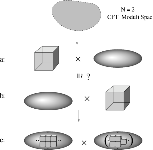
Figure 1: Models of the moduli space.

This picture was extended to that given in figure 1b after the discovery of mirror symmetry. Two Calabi-Yau spaces $X$ and $Y$ constitute a mirror pair if they yield isomorphic conformal theories when taken as the target space for a two-dimensional supersymmetric nonlinear $\sigma$-model, with the explicit isomorphism being a change in sign of the left moving $U(1)$ charges of all fields. Geometrically this implies that the Hodge numbers $h^{1,1}(X)$ and $h^{d-1,1}(X)$ are related to those of $Y$ by $h^{1,1}(X)=h^{d-1,1}(Y)$ and $h^{d-1,1}(X)=h^{1,1}(Y)$. Since the cohomology groups $H^{1,1}$ and $H^{d-1,1}$ correspond to Kähler and complex structure deformations, respectively, we see that the underlying conformal field theory moduli space has the two geometrical interpretations given in the figure. This immediately led to a problem since, as mentioned above, the geometric form of the moduli spaces of Kähler forms and complex structures appeared to be quite different.

This was resolved by the works of [1, 2, 3] to that shown in figure 1c. Here we see that the appropriate interpretation of the conformal field theory moduli space has required that the Kähler moduli space of $X$ be replaced by its “enlarged Kähler moduli space” (and similarly for $Y$). The latter contains numerous regions in addition to the Kähler cone of the topological manifold $X$. For instance, it typically contains regions corresponding to the Kähler cones of Calabi-Yau spaces related to $X$ by the birational operation of flopping a rational curve, regions corresponding to the moduli space of singular blow-downs of $X$ and its birational partners, and regions interpretable in terms of the parameter space of (gauged or ungauged) Landau-Ginzburg models fibered over various compact spaces. The complex structure moduli space can also be equipped with a phase structure [7] — as must happen to preserve mirror symmetry. We note that from the $\sigma$-model point of view the phase regions in the complex structure moduli space have a less pronounced physical interpretation. This is because in analyzing the $\sigma$-model we use perturbation theory in Kähler modes (which fix the size of the Calabi-Yau) and hence this approximation method is not mirror symmetric. However, the phase structure in the complex structure moduli space of $X$ is the phase structure in the enlarged Kähler moduli space of $Y$ and it is the latter interpretation where this phase structure is most manifest. For the purposes of this paper we may ignore the phase structure in the complex structure part of the moduli space and for this reason we have put parentheses around this in 1c.

The results of the present paper all stem directly from a careful study of the phase diagrams of figure 1c. We shall review the quantitative construction of these phase spaces in section 2; for now we will content ourselves with the schematic description given and summarize our results with a similar level of informality.

There are numerous ways of constructing $N=2$ superconformal theories with $c=3d$. Some constructions, such as the Calabi-Yau $\sigma$-models described above, are manifestly geometric in character. Other constructions do not begin with a geometrical target space and hence their geometrical content, if any, can only be assessed after more detailed study. More generally and pragmatically, given an abstract conformal field theory in some presentation, how do we determine if it has a geometrical interpretation? We will not seek to answer this question in generality, but rather will focus attention on those theories for which we can construct the phase diagram illustrated in figure 1c. For theories of this sort, as we shall review, toric geometry supplies us with a geometric description of each theory. We hasten to emphasize, though, that Calabi-Yau $\sigma$-models are but one kind of corresponding geometry. We will see, for instance, that Landau-Ginzburg orbifolds can be associated with noncompact, generally singular, configuration spaces.

From our brief discussion here and also from [1, 2, 3] one might think that any theory with a phase diagram such as that in figure 1c, has regions interpretable in terms of Calabi-Yau $\sigma$-models. After all, our progression from figures 1a through 1c has centered around Kähler cones of Calabi-Yau spaces. This conclusion, as we shall see in detail in section 3, is false and comes to bear on a number of issues, including that of the generality of mirror symmetry. Namely, there are Calabi-Yau manifolds that are rigid, i.e. that have trivial $H^{d-1,1}$. The mirror to such a space, therefore, should have $h^{1,1}=0$. This is troublesome, though, because Calabi-Yau spaces are Kähler and hence have at least one nontrivial element in $H^{1,1}$. With the above discussion, and explicit calculation in section 3, the resolution to this puzzle becomes clear: the enlarged Kähler moduli space for the theory mirror to the one associated with the rigid space $X$ does not contain a region interpretable in terms of a Calabi-Yau $\sigma$-model. In fact, the enlarged Kähler moduli space, in contrast to the generic case illustrated in figure 1c, is zero-dimensional and consists of a single point. By direct analysis, we show that the corresponding theory is a Landau-Ginzburg orbifold - not a Calabi-Yau $\sigma$-model - and hence it is perfectly consistent for the theory to lack a Kähler modulus. We note at the outset that possible resolutions to the question of the identity of mirrors to rigid Calabi-Yau spaces have been previously presented in [4, 5, 6]. These authors have invoked unexpected additional structures such as non-Calabi-Yau spaces of dimension greater than $d$ and supermanifolds in an attempt to resolve this issue. Contrary to these works, we see here that absolutely no additional structure is required. Rather, rigid Calabi-Yau manifolds fit perfectly into the general framework introduced in [1, 2, 3].

In addition to applying our analysis to the case of rigid Calabi-Yau manifolds and their mirrors, we also study two other interesting phenomena. First, we present an example of a theory with nonzero dimensional enlarged Kähler moduli space that does not contain a geometric region thus showing that the mere existence of a would-be Kähler form does not guarantee a Calabi-Yau interpretation. Second, we briefly discuss an example (first pointed out in [1]) whose enlarged Kähler moduli space has a phase whose target space has the desired dimension but is not of the Calabi-Yau type.

2 Phase Diagrams: Supersymmetric Gauge Theory and Toric Geometry

The moduli space of $N=2$ superconformal theories is most naturally interpretable in terms of a collection of regions within which the theory assumes a particular phase. Amongst the possibilities are smooth and singular geometric Calabi-Yau phases, gauged and ungauged Landau-Ginzburg phases, as well as orbifolds and hybrids thereof. This is the burden of figure 1c.

The existence and quantitative construction of these phase diagrams has been approached from two distinct vantage points in the works of [1] and [3]. In fact, a point which is not as fully appreciated as it might be is that these two approaches, although phrased in different languages, are isomorphic. Different questions, though, are often more easily answered from one of the two formalisms and hence it is important to fully understand both approaches and their precise relationship. It is the purpose of the present section to explain these issues. We note that the material in this section is implicit in [1] and [3]; for our purposes we need to make the relation explicit.

In brief, both [1] and [3] build constrained $N=2$ supersymmetric quantum field theories. In the physical approach of [1] these constraints are phrased in terms of symplectic quotients. In the mathematical approach of [3] these constraints are phrased in terms of holomorphic quotients. The well-known equivalence [8, 9] of these two approaches then implies that each constructs the same theory and hence also the same phase diagrams. The proper language for establishing these statements is that of toric geometry for which the reader can find a primer in [3]. In the following we will try to convey the main points with a minimum of unnecessary technical detail.

Complex projective space may be considered to be the prototypical toric variety. One constructs ${\mathchoice{\mbox{\bbbfont P}}{\mbox{\bbbfont P}}{\mbox{\smallbbbfont P}}{\mbox{\tinybbbfont P}}}^{n}$ by taking the $n+1$ homogeneous coordinates, $x_{i}$, spanning ${\mathchoice{\mbox{\bbbfont C}}{\mbox{\bbbfont C}}{\mbox{\smallbbbfont C}}{\mbox{\tinybbbfont C}}}^{n+1}$, removing the origin $x_{i}=0$ and modding out by the ${\mathchoice{\mbox{\bbbfont C}}{\mbox{\bbbfont C}}{\mbox{\smallbbbfont C}}{\mbox{\tinybbbfont C}}}^{*}$-action $x_{i}\to\lambda x_{i}$, $\lambda\neq 0$. A toric variety is simply a generalization of this concept with perhaps more than one ${\mathchoice{\mbox{\bbbfont C}}{\mbox{\bbbfont C}}{\mbox{\smallbbbfont C}}{\mbox{\tinybbbfont C}}}^{*}$-action and a possibly more complicated point set removed prior to the modding out process.

The most natural way of building a $N$=2 $\sigma$-model with a complex projective target space appears to be in terms of a $U(1)$-gauged field theory [10]. In this construction, one begins with the homogeneous coordinates, $x_{i}$, denoting chiral superfields, each with the same $U(1)$ charge, $Q_{i}$, (which we may take to be 1). The classical vacuum of such a theory may be determined by finding the minimum of the classical potential energy. Solving the algebraic equations for the auxiliary D-component of the gauge multiplet and including the result in the scalar potential yields the familiar contribution

$$(|x_{1}|^{2}+|x_{2}|^{2}+\ldots+|x_{n+1}|^{2}-r)^{2},$$ (1)

where $r$, a real number, is the coefficient of the familiar Fayet-Illiopoulos D-term. We take $r$ to be positive here to avoid naïvely breaking supersymmetry (see section 3.2 of [1] for a discussion on negative values of $r$). Minimizing the energy forces us to require that (1) should vanish. This immediately removes the origin $x_{i}=0$ from consideration. It also forces the $x_{i}$ to lie on the sphere $S^{2n+1}$. We may now divide out by the $U(1)$ (i.e., $S^{1}$) action to form $S^{2n+1}/S^{1}\cong{\mathchoice{\mbox{\bbbfont P}}{\mbox{\bbbfont P}}{\mbox{\smallbbbfont P}}{\mbox{\tinybbbfont P}}}^{n}$. The process of dividing by ${\mathchoice{\mbox{\bbbfont C}}{\mbox{\bbbfont C}}{\mbox{\smallbbbfont C}}{\mbox{\tinybbbfont C}}}^{*}$, in the usual formulation of ${\mathchoice{\mbox{\bbbfont P}}{\mbox{\bbbfont P}}{\mbox{\smallbbbfont P}}{\mbox{\tinybbbfont P}}}^{n}$ may be viewed to having taken place in two stages. First we fix an ${\mathchoice{\mbox{\bbbfont R}}{\mbox{\bbbfont R}}{\mbox{\smallbbbfont R}}{\mbox{\tinybbbfont R}}}_{+}$ degree of freedom by imposing the vanishing of (1) and then we divide out by $S^{1}$. The equivalence of these two constructions then follows from the fact that ${\mathchoice{\mbox{\bbbfont C}}{\mbox{\bbbfont C}}{\mbox{\smallbbbfont C}}{\mbox{\tinybbbfont C}}}^{*}\cong{\mathchoice{\mbox{\bbbfont R}}{\mbox{\bbbfont R}}{\mbox{\smallbbbfont R}}{\mbox{\tinybbbfont R}}}_{+}\times S^{1}$. Dividing by the former is a simple example of a holomorphic quotient; dividing by the latter is a simple example of a symplectic quotient. We have just seen, therefore, the essential reason why these two are equivalent. Let us now discuss how Witten generalized upon this quantum field theory approach of generating symplectic quotients. We will then discuss their equivalent holomorphic quotient description as in [3].

Witten [1] extended the above model to describe not a complex projective space but the “canonical” line bundle of complex projective space (see, for example, [11] for the precise definition of this bundle). Let us reserve $n$ to denote the dimension of the toric variety in question so now we are looking at a line bundle over ${\mathchoice{\mbox{\bbbfont P}}{\mbox{\bbbfont P}}{\mbox{\smallbbbfont P}}{\mbox{\tinybbbfont P}}}^{n-1}$ and the variable $x_{n+1}$ will now be treated differently to the others. This space is then built from ${\mathchoice{\mbox{\bbbfont C}}{\mbox{\bbbfont C}}{\mbox{\smallbbbfont C}}{\mbox{\tinybbbfont C}}}^{n+1}$ by removing the point $x_{1}=x_{2}=\ldots=x_{n}=0$ and modding out by the action

 

$${x_{i}}$$

  (2)

To produce this from the gauged $\sigma$-model point of view we put $Q_{i}=1$ for $i=1\ldots n$ and $Q_{n+1}=-n$.

The vanishing of the classical potential now implies

$$|x_{1}|^{2}+|x_{2}|^{2}+\ldots+|x_{n}|^{2}-n|x_{n+1}|^{2}=r.$$ (3)

We see that there are classical vacuum solutions for $r$ for either sign. If $r>0$, we thus recover the required target space as in the case of the projective space. If however $r<0$, we find that $x_{n+1}\neq 0$ and we have no condition on $x_{1},\ldots,x_{n}$. Let us consider this space more closely.

Removing the point set $x_{n+1}=0$ from ${\mathchoice{\mbox{\bbbfont C}}{\mbox{\bbbfont C}}{\mbox{\smallbbbfont C}}{\mbox{\tinybbbfont C}}}^{n+1}$ and dividing by the action (2) produces another toric variety. $x_{n+1}$ may be fixed by choosing a value for $\lambda^{n}$ leaving the $n$th roots of unity to act on the space spanned by $x_{1},\ldots,x_{n}$. Thus the toric variety is ${\mathchoice{\mbox{\bbbfont C}}{\mbox{\bbbfont C}}{\mbox{\smallbbbfont C}}{\mbox{\tinybbbfont C}}}^{n}/{\mathchoice{\mbox{\bbbfont Z}}{\mbox{\bbbfont Z}}{\mbox{\smallbbbfont Z}}{\mbox{\tinybbbfont Z}}}_{n}$. Therefore we see that the geometry of the target space can change discontinuously as we vary $r$. This theory is said to have two phases where the relevant toric variety is either the canonical line bundle of ${\mathchoice{\mbox{\bbbfont P}}{\mbox{\bbbfont P}}{\mbox{\smallbbbfont P}}{\mbox{\tinybbbfont P}}}^{n-1}$ or ${\mathchoice{\mbox{\bbbfont C}}{\mbox{\bbbfont C}}{\mbox{\smallbbbfont C}}{\mbox{\tinybbbfont C}}}^{n}/{\mathchoice{\mbox{\bbbfont Z}}{\mbox{\bbbfont Z}}{\mbox{\smallbbbfont Z}}{\mbox{\tinybbbfont Z}}}_{n}$.

The construction of [1] doesn’t quite stop here. One may introduce a $U(1)$-invariant superpotential, $W$, i.e., a ${\mathchoice{\mbox{\bbbfont C}}{\mbox{\bbbfont C}}{\mbox{\smallbbbfont C}}{\mbox{\tinybbbfont C}}}^{*}$-invariant polynomial over the $x_{i}$’s. Minimizing the classical potential now also implies that we are at a critical point of $W$.

Our toric “ambient” space will always turn out to be non-compact. This however will contain compact subspaces which may also be considered as toric varieties themselves. Clearly ${\mathchoice{\mbox{\bbbfont P}}{\mbox{\bbbfont P}}{\mbox{\smallbbbfont P}}{\mbox{\tinybbbfont P}}}^{n-1}$ is a toric subspace of the canonical line bundle over ${\mathchoice{\mbox{\bbbfont P}}{\mbox{\bbbfont P}}{\mbox{\smallbbbfont P}}{\mbox{\tinybbbfont P}}}^{n-1}$. The only compact toric subspace of ${\mathchoice{\mbox{\bbbfont C}}{\mbox{\bbbfont C}}{\mbox{\smallbbbfont C}}{\mbox{\tinybbbfont C}}}^{n}/{\mathchoice{\mbox{\bbbfont Z}}{\mbox{\bbbfont Z}}{\mbox{\smallbbbfont Z}}{\mbox{\tinybbbfont Z}}}_{n}$ is the point at the origin. Assuming that $W$ is suitably generic, the effect of including the superpotential term is to force the classical vacuum to be equal to, or contained in some compact toric subspace of the ambient space.

In our example, a suitable $W$ is $(x_{1}^{n}+x_{2}^{n}+\ldots+x_{n}^{n})x_{n+1}$. In the canonical line bundle over ${\mathchoice{\mbox{\bbbfont P}}{\mbox{\bbbfont P}}{\mbox{\smallbbbfont P}}{\mbox{\tinybbbfont P}}}^{n-1}$ case, the critical point set of $W$ consists of the hypersurface $x_{1}^{n}+x_{2}^{n}+\ldots+x_{n}^{n}=0$ in ${\mathchoice{\mbox{\bbbfont P}}{\mbox{\bbbfont P}}{\mbox{\smallbbbfont P}}{\mbox{\tinybbbfont P}}}^{n-1}$. This is a compact Calabi-Yau $(n-2)$-fold. This is thus named, the Calabi-Yau phase. In the ${\mathchoice{\mbox{\bbbfont C}}{\mbox{\bbbfont C}}{\mbox{\smallbbbfont C}}{\mbox{\tinybbbfont C}}}^{n}/{\mathchoice{\mbox{\bbbfont Z}}{\mbox{\bbbfont Z}}{\mbox{\smallbbbfont Z}}{\mbox{\tinybbbfont Z}}}_{n}$ case, the origin is the critical point set of $W$. Thus our classical vacuum is simply one point. The effective superpotential of this theory however allows for massless fluctuations around this point given by a Landau-Ginzburg superpotential $x_{1}^{n}+x_{2}^{n}+\ldots+x_{n}^{n}$. This is thus the Landau-Ginzburg phase. Note that all fluctuations around the vacuum in the Calabi-Yau phase are massive.

Let us fix some notation. We will call the ambient non-compact toric space $V_{\Delta}$. This contains a maximal compact toric subset $V_{\delta}$ (which may be reducible). Within $V_{\delta}$ we have the classical vacuum of the quantum field theory which we denote $X$.

A simple generalization of the above construction is to consider a weighted projective space for $V_{\delta}$. Clearly this may be achieved by giving different charges to $x_{1},\ldots,x_{n}$. Following the above formalism we would again obtain two phases depending on whether $r$ was less than or greater than zero. When we look at the associated conformal field theory it turns out that this does not capture the full moduli space, i.e., $h^{1,1}>1$ for many of these theories. It is not hard to generalize the present description to include at least some of these other degrees of freedom. For each such independent direction in the moduli space we are able to access in this formalism, we introduce a $U(1)$ gauge factor and a corresponding parameter $r_{l}$. Thus, the total gauge group is $G=U(1)^{s}$ where $s$ is the dimension of this subspace of the moduli space . The chiral fields will in general be charged under all of the $U(1)$ factors, and hence we write $Q_{i}^{(l)}$ to denote the charge of the $i^{th}$ chiral superfield under $U(1)_{(l)}$. The superpotential $W$ must now be a $G$-invariant combination of the chiral superfields.

It turns out that the language of toric geometry is precisely suited for determining all of the data needed for building such a model. Namely, in the case of $s=1$ (or more generally, $s$ is the number of distinct toric factors making up the ambient space) it is straightforward to figure out appropriate charges so that minimization of the scalar potential yields the desired model. When $s$ is not of this form, the problem requires a more systematic treatment; this is precisely what the formalism of toric geometry supplies. Furthermore, for these more general cases, it proves increasingly difficult to determine the phase diagram of the model by studying the minimum of the scalar potential for various values of the $r_{1},...,r_{s}$. The formalism of toric geometry, as described in [3], supplies us with a far more efficient means of determining the phase structure, as well. Hence, let us now recast the above formulation directly in terms of toric geometry.

The homogeneous coordinates (in the sense of [12]) $x_{1},\ldots,x_{N}$ form a natural representation of the group $({\mathchoice{\mbox{\bbbfont C}}{\mbox{\bbbfont C}}{\mbox{\smallbbbfont C}}{\mbox{\tinybbbfont C}}}^{*})^{N}$. Let us form a toric variety by removing some point set and dividing the resultant space by $({\mathchoice{\mbox{\bbbfont C}}{\mbox{\bbbfont C}}{\mbox{\smallbbbfont C}}{\mbox{\tinybbbfont C}}}^{*})^{N-n}$. Clearly the space formed, $V_{\Delta}$, is acted upon non-trivially by $({\mathchoice{\mbox{\bbbfont C}}{\mbox{\bbbfont C}}{\mbox{\smallbbbfont C}}{\mbox{\tinybbbfont C}}}^{*})^{n}$. Let us introduce $\zeta_{j}$, $j=1,\ldots,n$, as the natural representation of this $({\mathchoice{\mbox{\bbbfont C}}{\mbox{\bbbfont C}}{\mbox{\smallbbbfont C}}{\mbox{\tinybbbfont C}}}^{*})^{n}$-action. That is, the $\zeta_{j}$ provide coordinates on a dense open subset of $V_{\Delta}$. This follows since $V_{\Delta}$ may be regarded itself as a compactification of $({\mathchoice{\mbox{\bbbfont C}}{\mbox{\bbbfont C}}{\mbox{\smallbbbfont C}}{\mbox{\tinybbbfont C}}}^{*})^{n}$. Let us relate these new “affine” coordinates to the homogeneous coordinates by

$$\zeta_{j}=\prod_{i=1}^{N}x_{i}^{\alpha_{ij}},$$ (4)

where $\alpha_{ij}\in{\mathchoice{\mbox{\bbbfont Z}}{\mbox{\bbbfont Z}}{\mbox{\smallbbbfont Z}}{\mbox{\tinybbbfont Z}}}$. We may represent the $N\times n$ matrix, $\alpha_{ij}$, by a collection of $N$ points, which we denote A, living in an $n$-dimensional real space where $\alpha_{ij}$ is the $j$th coordinate of the $i$th point. Let us demand that A is such that there exists an $n$-dimensional lattice ${\bf N}$ within this same space (which we denote ${\bf N}_{{\mathchoice{\mbox{\bbbfont R}}{\mbox{\bbbfont R}}{\mbox{\smallbbbfont R}}{\mbox{\tinybbbfont R}}}}={\bf N}\otimes_{{\mathchoice{\mbox{\bbbfont Z}}{\mbox{\bbbfont Z}}{\mbox{\smallbbbfont Z}}{\mbox{\tinybbbfont Z}}}}{\mathchoice{\mbox{\bbbfont R}}{\mbox{\bbbfont R}}{\mbox{\smallbbbfont R}}{\mbox{\tinybbbfont R}}}$) such that

$${\mathchoice{\mbox{\scrfont A}}{\mbox{\scrfont A}}{\mbox{\smallscrfont A}}{\mbox{\tinyscrfont A}}}={\bf N}\cap(\hbox{Convex hull of ${\mathchoice{\mbox{\scrfont A}}{\mbox{\scrfont A}}{\mbox{\smallscrfont A}}{\mbox{\tinyscrfont A}}}$}\,).$$ (5)

The notation $\alpha_{i}$ will denote the position vector of the $i$th point of A in ${\bf N}$.

Consider now the charges of the homogeneous coordinates under the $({\mathchoice{\mbox{\bbbfont C}}{\mbox{\bbbfont C}}{\mbox{\smallbbbfont C}}{\mbox{\tinybbbfont C}}}^{*})^{N-n}$ by which we modded out. Denote these $Q_{i}^{(l)}$ where $i=1,\ldots,N$ and $l=1,\ldots,N-n$. The obvious short exact sequence

$$1\to({\mathchoice{\mbox{\bbbfont C}}{\mbox{\bbbfont C}}{\mbox{\smallbbbfont C}}{\mbox{\tinybbbfont C}}}^{*})^{n}\to({\mathchoice{\mbox{\bbbfont C}}{\mbox{\bbbfont C}}{\mbox{\smallbbbfont C}}{\mbox{\tinybbbfont C}}}^{*})^{N}\to({\mathchoice{\mbox{\bbbfont C}}{\mbox{\bbbfont C}}{\mbox{\smallbbbfont C}}{\mbox{\tinybbbfont C}}}^{*})^{N-n}\to 1,$$ (6)

induces,

$$\sum_{i=1}^{N}Q^{(l)}_{i}\alpha_{ij}=0,\quad\forall l,j.$$ (7)

Thus, we see that the charges $Q^{(l)}_{i}$ are simply the kernel of the transpose of the matrix whose elements are $\alpha_{ij}$. The reader should check that in the simple case, say, of projective space discussed earlier, that the charge assignment posited can in fact be derived in this manner.

Now define ${\bf M}$ as the dual lattice to ${\bf N}$. Let us demand that there is an element $\mu\in{\bf M}$ such that

$$\langle\mu,\alpha_{i}\rangle=1,\quad\forall i.$$ (8)

This condition is similar to stating that $V_{\Delta}$ be a space with vanishing canonical class, $K$, (or zero first Chern class). Actually $V_{\Delta}$ need not be smooth so be need to be more careful about our language. The correct term from algebraic geometry is that $V_{\Delta}$ is Gorenstein (see, for example, [13]). Applying (8) to (7) tells us that

$$\sum_{i=1}^{N}Q^{(l)}_{i}=0,\quad\forall l.$$ (9)

This appears as an important condition in [1] ensuring freedom from anomalies in certain chiral currents which should be present if there is an infrared limit with $N$=2 superconformal invariance. It is curious to note that (9) is not sufficient to guarantee (8). We may have $\langle\mu,\alpha_{i}\rangle=k$ for example, for some integer $k$. $V_{\Delta}$ would then be ℚ-Gorenstein which is roughly saying that $kK=0$ but $K$ may be a non-trivial torsion element. The effect of this in terms of the two dimension quantum field theory has not been studied.

This point set A gives us all the information we require to build $V_{\Delta}$ except which point set should be removed from $({\mathchoice{\mbox{\bbbfont C}}{\mbox{\bbbfont C}}{\mbox{\smallbbbfont C}}{\mbox{\tinybbbfont C}}}^{*})^{N}$ before performing the quotient. This is performed in toric geometry by building a fan, $\Delta$. A fan is a collection of tesselating cones in ${\bf N}_{\mathchoice{\mbox{\bbbfont R}}{\mbox{\bbbfont R}}{\mbox{\smallbbbfont R}}{\mbox{\tinybbbfont R}}}$ with apexes at the origin. The intersection of this fan with the hyperplane containing A will be a set of tesselating polytopes. The convex hull of this set of polytopes must be the convex hull of A and the vertices of the polytopes must be elements of A. Thus each cone, $\sigma$, in $\Delta$ is “generated” by a subset of A. We say $\alpha_{i}\in\sigma$ if $\alpha_{i}$ is one of the generators, i.e., $\alpha_{i}$ lies at a vertex of the intersection of $\sigma$ with the hyperplane in ${\bf N}_{\mathchoice{\mbox{\bbbfont R}}{\mbox{\bbbfont R}}{\mbox{\smallbbbfont R}}{\mbox{\tinybbbfont R}}}$ containing A. The point set $F_{\Delta}$ removed from ${\mathchoice{\mbox{\bbbfont C}}{\mbox{\bbbfont C}}{\mbox{\smallbbbfont C}}{\mbox{\tinybbbfont C}}}^{N}$ prior to quotienting is then specified by

$$\bigcap_{\sigma\in\Delta}\Bigl{\{}x\in{\mathchoice{\mbox{\bbbfont C}}{\mbox{\bbbfont C}}{\mbox{\smallbbbfont C}}{\mbox{\tinybbbfont C}}}^{N};\prod_{{\alpha_{i}\in{\mathchoice{\mbox{\scrfont A}}{\mbox{\scrfont A}}{\mbox{\smallscrfont A}}{\mbox{\tinyscrfont A}}},}\atop{\alpha_{i}\not\in\sigma}}\!\!x_{i}=0\Bigr{\}},$$ (10)

where $x$ is the point with coordinates $x_{i}$.

The fact that different fans may be associated with the point-set A gives rise to the phase structure. We need only consider the case where all the $\sigma$’s are simplicial based cones, i.e., we induce a simplicial decomposition of triangulation of A. To each such fan (satisfying in addition a certain “convexity” property, see [3] for more details) we associate a phase. Other fans consistent with A not satisfying these conditions may always be considered as models on the boundary between two or more phases. The parameters, $r$, in the linear $\sigma$-model approach give us an identical fan structure. This is best understood from examining figure 11 of [3]. The $r$ parameters, in essence, fix the heights of the points in this figure and hence following the discussion of section of 3.8 of [3] their values determine a triangulation of the point set A. From a physical point of view we can group together those values for the $r$ parameters which yield the same phase for the model. In this way we partition the space of all possible $r$’s into a phase diagram. This phase diagram is the “secondary fan” for the moduli space as discussed in [3].

We now have a dictionary between [1] and the toric approach: Specifying generic values of “$r$” parameters is equivalent to specifying a triangulation of A. The non-vanishing conditions on the fields $x_{i}$ specified by minimizing the $D$-term part of the classical potential is equivalent to removing the point set $F_{\Delta}$ given by (10).

Note that requiring A to be “complete” in the sense of (5) is not necessary in the analysis of [1]. By imposing this condition we gain access to the largest subspace of the moduli space we can reach by this toric method.

One point in the dictionary between [1] and the toric approach which we have not spelled out explicitly as yet is how we determine the superpotential $W$ from the toric data. This is straightforward as we now describe. Let us $G$ to denote the group $({\mathchoice{\mbox{\bbbfont C}}{\mbox{\bbbfont C}}{\mbox{\smallbbbfont C}}{\mbox{\tinybbbfont C}}}^{*})^{N-n}$. $W$ is a $G$-invariant polynomial in the chiral superfields. From (7) we see that any monomial of the form

$$\prod_{i=1}^{N}x_{i}^{\langle\alpha_{i},v\rangle}$$ (11)

for a fixed but arbitrary vector $v$ is $G$-invariant. However, we want all terms in $W$ to not only be $G$-invariant but also to have nonnegative integral exponents. Towards this end we are naturally led to introduce the cone $\Upsilon$ in ${\bf M}_{\mathchoice{\mbox{\bbbfont R}}{\mbox{\bbbfont R}}{\mbox{\smallbbbfont R}}{\mbox{\tinybbbfont R}}}$, dual to $\Sigma$ which is the cone over the convex hull of A in ${\bf N}_{\mathchoice{\mbox{\bbbfont R}}{\mbox{\bbbfont R}}{\mbox{\smallbbbfont R}}{\mbox{\tinybbbfont R}}}$, defined by

$$\Upsilon=\left\{s\in{\bf M}_{\mathchoice{\mbox{\bbbfont R}}{\mbox{\bbbfont R}}{\mbox{\smallbbbfont R}}{\mbox{\tinybbbfont R}}};\langle s,t\rangle\geq 0,\forall t\in\Sigma\right\}.$$ (12)

The integral lattice points in $\Upsilon$, when substituted for the vector $v$ in (11), will then generate $G$-invariant monomials with nonnegative exponents. To systematize this, we now define ${\mathchoice{\mbox{\scrfont B}}{\mbox{\scrfont B}}{\mbox{\smallscrfont B}}{\mbox{\tinyscrfont B}}}\,{}^{\prime}\subset\Upsilon$ by

$${\mathchoice{\mbox{\scrfont B}}{\mbox{\scrfont B}}{\mbox{\smallscrfont B}}{\mbox{\tinyscrfont B}}}\,{}^{\prime}={\bf M}\cap\Upsilon,$$ (13)

the integral lattice points contained in the dual cone. Any point in ${\mathchoice{\mbox{\scrfont B}}{\mbox{\scrfont B}}{\mbox{\smallscrfont B}}{\mbox{\tinyscrfont B}}}\,{}^{\prime}$, if substituted for the vector $v$ in (11), yields a $G$-invariant nonnegative exponent monomial. Finally, we note that we would like $W$ to be a suitably “quasihomogeneous” polynomial of lowest nontrivial degree in the $x_{i}$. This will remove any “irrelevant” terms in the superpotential [14] and may be achieved as follows. Let the monomials in this reduced superpotentials be labeled by elements of ${\mathchoice{\mbox{\scrfont B}}{\mbox{\scrfont B}}{\mbox{\smallscrfont B}}{\mbox{\tinyscrfont B}}}\subset{\mathchoice{\mbox{\scrfont B}}{\mbox{\scrfont B}}{\mbox{\smallscrfont B}}{\mbox{\tinyscrfont B}}}\,{}^{\prime}$. Following [15] let us put one last condition on A, namely that when we derive the point set B exists a vector $\nu\in{\bf N}$ such that

$$\langle\beta_{v},\nu\rangle=1,\quad\forall\beta_{v}\in{\mathchoice{\mbox{\scrfont B}}{\mbox{\scrfont B}}{\mbox{\smallscrfont B}}{\mbox{\tinyscrfont B}}},$$ (14)

and that the vectors given by the elements of B (or a subset of B) generate $\Upsilon$. We also impose the condition on B paralleling our discussion for the point set A. Namely, we can say

$${\mathchoice{\mbox{\scrfont B}}{\mbox{\scrfont B}}{\mbox{\smallscrfont B}}{\mbox{\tinyscrfont B}}}={\bf M}\cap(\hbox{Convex hull of ${\mathchoice{\mbox{\scrfont B}}{\mbox{\scrfont B}}{\mbox{\smallscrfont B}}{\mbox{\tinyscrfont B}}}$}\,),$$ (15)

with the elements of B at the vertices of this convex hull generating $\Upsilon$. We denote by $M$ the number of points in B so that $v=1,\ldots,M$. The superpotential $W$ is then constructed according to

$$W=\sum_{v=1}^{M}a_{v}w_{v},$$ (16)

for $a_{v}\in{\mathchoice{\mbox{\bbbfont C}}{\mbox{\bbbfont C}}{\mbox{\smallbbbfont C}}{\mbox{\tinybbbfont C}}}$ with

$$w_{v}=\prod_{i=1}^{N}x_{i}^{\langle\beta_{v},\alpha_{i}\rangle}.$$ (17)

We may note at this point that mirror symmetry is conjectured to exchange the sets $\{{\bf M},\mu,M,{\mathchoice{\mbox{\scrfont A}}{\mbox{\scrfont A}}{\mbox{\smallscrfont A}}{\mbox{\tinyscrfont A}}}\,\}\leftrightarrow\{{\bf N},\nu,N,{\mathchoice{\mbox{\scrfont B}}{\mbox{\scrfont B}}{\mbox{\smallscrfont B}}{\mbox{\tinyscrfont B}}}\}$. This may be regarded as a generalization of the “monomial-divisor mirror map” of [16]. The mirror pairs of [18] (which is established at the conformal field theory level) are a subset of this general construction and the examples in sections 3.2 and 3.3 are in this subset. Thus statement concerning mirror symmetry with regards to these examples may be regarded as definitely true. Also note that our analysis of the phases of the moduli space does not depend on the mirror map and thus does not depend on this mirror conjecture.

Now let us try to calculate the central charge $3d$ of the conformal field theory associated to this model. We may apply the same reasoning as was used in [14] to determine this. Firstly we have $N$ chiral superfields each of which contributes $+1$ to $d$. This may be taken to correspond to the string propagating in ${\mathchoice{\mbox{\bbbfont C}}{\mbox{\bbbfont C}}{\mbox{\smallbbbfont C}}{\mbox{\tinybbbfont C}}}^{N}$. We also have $N-n$ vector superfields which we take to contribute $-1$ to $d$ since each removes one complex dimension from the target space. Thus, so far we have $d=n$. However, the string is further confined by the superpotential $W$ and we expect this to reduce the value of $d$ as we now show.

Consider now rescaling by an element of $({\mathchoice{\mbox{\bbbfont C}}{\mbox{\bbbfont C}}{\mbox{\smallbbbfont C}}{\mbox{\tinybbbfont C}}}^{*})^{N}$,

$$x_{i}\to\lambda^{\omega_{i}}x_{i}.$$ (18)

The monomial $w_{v}$ then scales to $\lambda^{\chi}w_{v}$ where

$$\chi=\sum_{i=1}^{N}\langle\beta_{v},\alpha_{i}\rangle\omega_{i}.$$ (19)

Consider choosing the weights $\omega_{i}$ such that

$$\sum_{i=1}^{N}\omega_{i}\alpha_{i}=\nu.$$ (20)

Then all the monomials transform $w_{v}\to\lambda w_{v}$ and thus, declaring $a_{v}$ to be invariant, we have $W\to\lambda W$. Taking the inner product of (20) with $\mu$ gives

$$\sum_{i=1}^{N}\omega_{i}=\langle\mu,\nu\rangle.$$ (21)

It was shown in [14] that the effect of the superpotential is to contribute $-2\sum\omega_{i}$ to $d$. Thus we have

$$d=n-2\langle\mu,\nu\rangle,$$ (22)

in agreement with the conjecture in [15].

For the cases considered in [3] based upon the construction of [19] we had $\langle\mu,\nu\rangle=1$. This then is a generalization. It should be noted that this more generalized picture could have been deduced directly by applying the toric language to Witten’s formulation of [1] although historically it was first written in the form of [20] where it was used specifically for conjecturing the mirror map for complete intersections in toric varieties.

To summarize so far, all the data we require to build an abelian gauged linear $\sigma$-model of the form studied in [1] is the matrix $\alpha_{ij}$. To provide a consistent model for a conformal field theory we demand that this matrix be compatible with $\mu$ and $\nu$ and be consistent with the existence of ${\bf N}$ in the form of (5). Once we have this information we may apply the technology of [1, 3] to determine the geometry of the various phases in the moduli space of Kähler forms. This is most easily determined in terms of triangulations of the point set A.

There is one more piece of information we will need before moving on to some examples concerning orbifolding. The toric variety $V_{\Delta}$ is acted upon by $({\mathchoice{\mbox{\bbbfont C}}{\mbox{\bbbfont C}}{\mbox{\smallbbbfont C}}{\mbox{\tinybbbfont C}}}^{*})^{n}$. It is simple in toric geometry to describe the orbifold of $V_{\Delta}$ by a discrete subgroup of this $({\mathchoice{\mbox{\bbbfont C}}{\mbox{\bbbfont C}}{\mbox{\smallbbbfont C}}{\mbox{\tinybbbfont C}}}^{*})^{n}$. Consider the affine coordinates introduced by (4). Let us consider the element, $g\in({\mathchoice{\mbox{\bbbfont C}}{\mbox{\bbbfont C}}{\mbox{\smallbbbfont C}}{\mbox{\tinybbbfont C}}}^{*})^{n}$ which acts by

$$g:(\zeta_{1},\zeta_{2},\ldots,\zeta_{n})\mapsto(e^{2\pi ig_{1}}\zeta_{1},e^{2\pi ig_{2}}\zeta_{2},\ldots,e^{2\pi ig_{n}}\zeta_{n})$$ (23)

where $0\leq g_{j}<1$. We can see (for more details consult [21]) that dividing $V_{\Delta}$ by the group generated by $g$ is equivalent to replacing the lattice ${\bf N}$ by a lattice generated by ${\bf N}$ and the vector $(g_{1},g_{2},\ldots,g_{n})\in{\bf N}_{\mathchoice{\mbox{\bbbfont R}}{\mbox{\bbbfont R}}{\mbox{\smallbbbfont R}}{\mbox{\tinybbbfont R}}}$. The reason for this is that lattice points $p$ in ${\bf N}$ represent one (complex) parameter group actions on the toric variety

$$p:(\zeta_{1},\zeta_{2},\ldots,\zeta_{n})\mapsto(\lambda^{p_{1}}\zeta_{1},\lambda^{p_{2}}\zeta_{2},\ldots,\lambda^{p_{n}}\zeta_{n}).$$ (24)

For points $p$ whose components are non-integral, such a map is only well defined if certain global identifications are made on the $(\zeta_{1},\zeta_{2},\ldots,\zeta_{n})$. In particular, one directly sees that taking $p$ to be $(g_{1},g_{2},\ldots,g_{n})$ requires the desired identification of (23).

3 Applications

Let us now illustrate the general method of the previous section by applying it to various examples. The possibilities offered by this formulation appear to be very rich but we select here a few key examples to emphasize points relevant to our discussion.

3.1 The Hypersurface Case

Suppose that $\langle\mu,\nu\rangle=1$. In this case it is easy to see that $\nu\in{\mathchoice{\mbox{\scrfont A}}{\mbox{\scrfont A}}{\mbox{\smallscrfont A}}{\mbox{\tinyscrfont A}}}$ and that this point lies properly in the interior of the convex hull of A (since $\langle\beta_{v},\nu\rangle$ is strictly positive). One possible triangulation of the point set A thus consists of drawing lines from $\nu$ to each point on the vertices of the convex hull and filling this skeleton in with a suitable set of simplices to form a triangulation. The resultant set forms a complete fan of dimension $n-1$ with center $\nu$. This fan $\delta$ corresponds to a compact $(n-1)$-dimensional toric sub-variety $V_{\delta}$ of $V_{\Delta}$. Let us denote by $p$ the homogeneous coordinate corresponding to $\nu$. We see from (17) that every term in the superpotential appears linearly in $p$. Thus we may write $W=pG$ where $G$ is a function of the $N-1$ homogeneous coordinates describing $V_{\delta}$. Thus the condition $\partial W/\partial p=0$ implies $G=0$ — i.e., we are on a hypersurface within $V_{\delta}$. For a generic $G$, the other derivatives of $W$ imply that $p=0$.

The target space, $X$, is now a hypersurface within $V_{\delta}$ which itself has dimension $n-1$. $X$ is thus of dimension $n-2$. The equation (22) tells us that $d=n-2$. In fact $X$ is an anticanonical divisor of $V_{\delta}$ [19] and is thus a Calabi-Yau space of $d$ dimensions. Note that $X$ may not be smooth but these singularities can often be removed by further refinements of the fan $\delta$. Actually, in the case $d\leq 3$ the singularities may always be removed in this way.

For the case $\langle\mu,\nu\rangle=1$ we therefore always have a “Calabi-Yau” phase. That is, some limit in the moduli space where we may go to build some non-linear $\sigma$-model of the conformal field theory (although in case $d>3$ we may have to include considerations such as terminal orbifold singularities in our model). The case considered here is basically of the type studied in [19, 3] as shown in [15]. It also includes the example of the model with the Landau-Ginzburg phase in ${\mathchoice{\mbox{\bbbfont C}}{\mbox{\bbbfont C}}{\mbox{\smallbbbfont C}}{\mbox{\tinybbbfont C}}}^{n}/{\mathchoice{\mbox{\bbbfont Z}}{\mbox{\bbbfont Z}}{\mbox{\smallbbbfont Z}}{\mbox{\tinybbbfont Z}}}_{n}$ and the Calabi-Yau hypersurface in ${\mathchoice{\mbox{\bbbfont P}}{\mbox{\bbbfont P}}{\mbox{\smallbbbfont P}}{\mbox{\tinybbbfont P}}}^{n-1}$ discussed above.

3.2 The Mirror of the Z-orbifold

We now turn to the issue of rigid Calabi-Yau spaces and their mirrors. For concreteness we focus on the Z-orbifold of [22]. Recall that this is the torus of six real dimensions divided by a diagonal ${\mathchoice{\mbox{\bbbfont Z}}{\mbox{\bbbfont Z}}{\mbox{\smallbbbfont Z}}{\mbox{\tinybbbfont Z}}}_{3}$ action. It has 36 (1,1)-forms (9 from the original torus and 27 associated with blow up modes) and no (2,1)-forms. It is therefore rigid. Using the construction of [18], it was shown in [23] how to construct the Z-orbifold in terms of an orbifold of a Gepner model [24]. To phrase this more carefully allowing for the phase structure, one builds a conformal field theory as an orbifold of a Gepner model which may be deformed via marginal operators to a theory corresponding to a $\sigma$-model whose target space is the blown-up Z-orbifold. It was also shown how to build a conformal field theory giving the mirror of the above theory, also as a orbifold of the Gepner model.

The Gepner model itself is believed to be equivalent to an orbifold of a Landau-Ginzburg theory. In the case under consideration (the ${\bf 1}^{9}$ model) the configuration space of this Landau-Ginzburg orbifold theory is ${\mathchoice{\mbox{\bbbfont C}}{\mbox{\bbbfont C}}{\mbox{\smallbbbfont C}}{\mbox{\tinybbbfont C}}}^{9}/{\mathchoice{\mbox{\bbbfont Z}}{\mbox{\bbbfont Z}}{\mbox{\smallbbbfont Z}}{\mbox{\tinybbbfont Z}}}_{3}$. The space ${\mathchoice{\mbox{\bbbfont C}}{\mbox{\bbbfont C}}{\mbox{\smallbbbfont C}}{\mbox{\tinybbbfont C}}}^{9}$ is a toric variety with $n=9$ described simply by the fan consisting of one cone, $\sigma$, isomorphic to the positive quadrant of ${\mathchoice{\mbox{\bbbfont R}}{\mbox{\bbbfont R}}{\mbox{\smallbbbfont R}}{\mbox{\tinybbbfont R}}}^{9}$. That is, A consists of the points $(1,0,0,0,0,0,0,0,0),(0,1,0,0,0,0,0,0,0),\ldots,(0,0,0,0,0,0,0,0,1)$. The required ${\mathchoice{\mbox{\bbbfont Z}}{\mbox{\bbbfont Z}}{\mbox{\smallbbbfont Z}}{\mbox{\tinybbbfont Z}}}_{3}$ quotient is performed by adding the generator

$$g_{1}=({\textstyle\frac{1}{3}},{\textstyle\frac{1}{3}},{\textstyle\frac{1}{3}},{\textstyle\frac{1}{3}},{\textstyle\frac{1}{3}},{\textstyle\frac{1}{3}},{\textstyle\frac{1}{3}},{\textstyle\frac{1}{3}},{\textstyle\frac{1}{3}}),$$ (25)

to the integral lattice of ${\mathchoice{\mbox{\bbbfont R}}{\mbox{\bbbfont R}}{\mbox{\smallbbbfont R}}{\mbox{\tinybbbfont R}}}^{9}$. It was shown in [23] that the mirror of the Z-orbifold was obtained by dividing by a further ${\mathchoice{\mbox{\bbbfont Z}}{\mbox{\bbbfont Z}}{\mbox{\smallbbbfont Z}}{\mbox{\tinybbbfont Z}}}_{3}$ (i.e., taking a ${\mathchoice{\mbox{\bbbfont Z}}{\mbox{\bbbfont Z}}{\mbox{\smallbbbfont Z}}{\mbox{\tinybbbfont Z}}}_{3}$ orbifold of the Gepner model) given by the vector

$$g_{2}=(0,0,0,{\textstyle\frac{1}{3}},{\textstyle\frac{1}{3}},{\textstyle\frac{1}{3}},{\textstyle\frac{2}{3}},{\textstyle\frac{2}{3}},{\textstyle\frac{2}{3}}),$$ (26)

to give the required ${\bf N}$-lattice. We may apply a $Gl(9,{\mathchoice{\mbox{\bbbfont R}}{\mbox{\bbbfont R}}{\mbox{\smallbbbfont R}}{\mbox{\tinybbbfont R}}})$ transformation to ${\bf N}_{\mathchoice{\mbox{\bbbfont R}}{\mbox{\bbbfont R}}{\mbox{\smallbbbfont R}}{\mbox{\tinybbbfont R}}}$ to rotate ${\bf N}$ back into the standard integral lattice. This will act on $\sigma$ so that it is no longer the positive quadrant. One choice of transformation leaves $\sigma$ generated by

 

$${\alpha_{1}}$$

  (27)

These 9 points lie in the hyperplane defined by $\mu=(3,1,1,1,1,1,1,1,3)$. It is a simple matter to show that the dual cone gives $\nu=(1,0,0,0,0,0,0,0,0)$ so that A has the required properties.

The important property of this model stems from the fact that the points $\alpha_{1},\ldots,\alpha_{9}$ form the vertices of a simplex with no interior points lying on the lattice ${\bf N}$. That is, the set A consists only of those points listed in (27). Thus the only triangulation of A consists of this simplex! This model has $V_{\Delta}\cong{\mathchoice{\mbox{\bbbfont C}}{\mbox{\bbbfont C}}{\mbox{\smallbbbfont C}}{\mbox{\tinybbbfont C}}}^{9}/({\mathchoice{\mbox{\bbbfont Z}}{\mbox{\bbbfont Z}}{\mbox{\smallbbbfont Z}}{\mbox{\tinybbbfont Z}}}_{3}\times{\mathchoice{\mbox{\bbbfont Z}}{\mbox{\bbbfont Z}}{\mbox{\smallbbbfont Z}}{\mbox{\tinybbbfont Z}}}_{3})$ with superpotential

$$W=a_{1}x_{1}^{3}+a_{2}x_{2}^{3}+\ldots+a_{9}x_{9}^{3}+a_{10}x_{1}x_{2}x_{3}+\ldots.$$ (28)

The critical point of $W$ is the origin. Thus we have an orbifold of a Landau-Ginzburg theory as expected. Since there is no other triangulation of A there is no other phase and, in particular, no Calabi-Yau phase. Since $\langle\mu,\nu\rangle=3$ we are not in conflict with the section 3.1. As expected we see that $d=3$ in agreement with the fact that this theory is the mirror of a smooth Calabi-Yau threefold (i.e., the blow-up of the Z-orbifold).

Thus, by properly understanding the full content of mirror symmetry — as a symmetry between the moduli spaces of $N=2$ superconformal theories — we see that there is no puzzle regarding the mirror of a rigid Calabi-Yau manifold. The mirror description simply does not have a Calabi-Yau phase and hence the absence of a Kähler form causes no conflict.

It is important to realize that we have all the information we need to study this model without recourse to finding some other effective target space geometry. In particular, deformations of complex structure are achieved by deforming the $a_{v}$ parameters in (28) in the usual way and one may then use mirror symmetry to study the moduli space of Kähler forms of the Z-orbifold as was done in [4].

The lack of a Calabi-Yau phase appears due to the existence of terminal singularities in algebraic geometry as we now discuss (see also [21] for a more thorough account). In section 2 we discussed the case of a Landau-Ginzburg theory in ${\mathchoice{\mbox{\bbbfont C}}{\mbox{\bbbfont C}}{\mbox{\smallbbbfont C}}{\mbox{\tinybbbfont C}}}^{n}/{\mathchoice{\mbox{\bbbfont Z}}{\mbox{\bbbfont Z}}{\mbox{\smallbbbfont Z}}{\mbox{\tinybbbfont Z}}}_{n}$. In this case, the ${\mathchoice{\mbox{\bbbfont Z}}{\mbox{\bbbfont Z}}{\mbox{\smallbbbfont Z}}{\mbox{\tinybbbfont Z}}}_{n}$ symmetry is generated by $({\textstyle\frac{1}{n}},{\textstyle\frac{1}{n}},\ldots)$. This singularity may be blown-up to give the canonical line bundle over ${\mathchoice{\mbox{\bbbfont P}}{\mbox{\bbbfont P}}{\mbox{\smallbbbfont P}}{\mbox{\tinybbbfont P}}}^{n-1}$. This smooth space has trivial canonical class. Thus the singularity ${\mathchoice{\mbox{\bbbfont C}}{\mbox{\bbbfont C}}{\mbox{\smallbbbfont C}}{\mbox{\tinybbbfont C}}}^{n}/{\mathchoice{\mbox{\bbbfont Z}}{\mbox{\bbbfont Z}}{\mbox{\smallbbbfont Z}}{\mbox{\tinybbbfont Z}}}_{n}$ may be blown up without adding something non-trivial into the canonical class. Such a blow-up mode is always visible in the associated conformal field theory as a truly marginal operator since it may be regarded as a deformation of the Kähler form.

A terminal singularity is a singularity which cannot be resolved (or even partially resolved) without adding something non-trivial to the canonical class. The singularity ${\mathchoice{\mbox{\bbbfont C}}{\mbox{\bbbfont C}}{\mbox{\smallbbbfont C}}{\mbox{\tinybbbfont C}}}^{9}/{\mathchoice{\mbox{\bbbfont Z}}{\mbox{\bbbfont Z}}{\mbox{\smallbbbfont Z}}{\mbox{\tinybbbfont Z}}}_{3}$ generated by $g_{1}$ of (25) is precisely such a singularity. As such, from the conformal field theory point of view, it is “stuck”. This agrees with the fact that the Gepner model contains no marginal operators corresponding to deformations of the Kähler form.

One can go ahead and blow-up the ${\mathchoice{\mbox{\bbbfont C}}{\mbox{\bbbfont C}}{\mbox{\smallbbbfont C}}{\mbox{\tinybbbfont C}}}^{9}/{\mathchoice{\mbox{\bbbfont Z}}{\mbox{\bbbfont Z}}{\mbox{\smallbbbfont Z}}{\mbox{\tinybbbfont Z}}}_{3}$ singularity if one really desires some smooth manifold. There is no unique prescription for this but one may, for example, form the space ${\cal O}_{{\mathchoice{\mbox{\bbbfont P}}{\mbox{\bbbfont P}}{\mbox{\smallbbbfont P}}{\mbox{\tinybbbfont P}}}^{8}}(-3)$. This is a line bundle over ${\mathchoice{\mbox{\bbbfont P}}{\mbox{\bbbfont P}}{\mbox{\smallbbbfont P}}{\mbox{\tinybbbfont P}}}^{8}$ with $K<0$ (i.e., $c_{1}>0$). The homogeneous coordinates of this projective space may be given by the coordinates of the original ${\mathchoice{\mbox{\bbbfont C}}{\mbox{\bbbfont C}}{\mbox{\smallbbbfont C}}{\mbox{\tinybbbfont C}}}^{9}$. The superpotential of the Landau-Ginzburg theory is cubic in these fields and so one might try to associate this model to the cubic hypersurface in ${\mathchoice{\mbox{\bbbfont P}}{\mbox{\bbbfont P}}{\mbox{\smallbbbfont P}}{\mbox{\tinybbbfont P}}}^{8}$. This is the essence of the construction of [4, 5]. Note that in the language of this paper, we no longer satisfy (9) and so our field theory is expected to have undesirable properties in the infrared limit.

When we try to describe the mirror of the Z-orbifold, the situation becomes even worse. The second ${\mathchoice{\mbox{\bbbfont Z}}{\mbox{\bbbfont Z}}{\mbox{\smallbbbfont Z}}{\mbox{\tinybbbfont Z}}}_{3}$ quotient given by $g_{2}$ induces further terminal quotient singularities on ${\mathchoice{\mbox{\bbbfont P}}{\mbox{\bbbfont P}}{\mbox{\smallbbbfont P}}{\mbox{\tinybbbfont P}}}^{8}$ which require considerably more to be added to the canonical class. We hope the reader sees that this procedure of forcing a smooth geometrical interpretation when terminal singularities appear is completely unnatural when written in terms of the underlying conformal field theory and it is unnecessary when one adopts the phase picture. The mirror of the Z-orbifold need only be described as an orbifold of a Landau-Ginzburg theory in ${\mathchoice{\mbox{\bbbfont C}}{\mbox{\bbbfont C}}{\mbox{\smallbbbfont C}}{\mbox{\tinybbbfont C}}}^{9}$.

We should add that the construction of [6] should be expected to overcome the renormalization group flow problem inherent in the above hypersurface in ${\mathchoice{\mbox{\bbbfont P}}{\mbox{\bbbfont P}}{\mbox{\smallbbbfont P}}{\mbox{\tinybbbfont P}}}^{8}$ of [4, 5]. In the construction of [6] one adds ghost fields to reduce the effective dimension of the target space back down to that of $d$. Assuming this is the case, this target space with ghosts can be proposed as a good geometric interpretation of the conformal field theory. It should be pointed out however that such geometric interpretations are probably highly ambiguous. That is, one conformal field theory can be given many interpretations. This occurs in [6] where constructions of K3 conformal field theories are given in terms of a 4 complex dimensional space with ghosts whereas the complete moduli space is already understood completely in terms of K3 surfaces [25]. In fact, it is probable that any geometric model may be blown-up to give $K<0$ and then nonzero contributions the the $\beta$-function be cancelled by adding suitable extra fields. Since there are an infinite number of such blow-ups for any model there is the possibility of ascribing an infinity of geometric interpretations of this form.

Finally note that it might be possible to associate some geometry with the case discussed in this section by considering orbifolds with discrete torsion [26]. Since we do not understand precisely how to relate quotient singularities with discrete torsion to classical singularities we will not discuss this interpretation here.

3.3 A Case with $h^{1,1}=1$

The above example may be considered rather trivial in that our phase space was zero dimensional, i.e., consisted of only one point. Let us now give a less trivial example which still has no Calabi-Yau phase.

Consider dividing ${\mathchoice{\mbox{\bbbfont C}}{\mbox{\bbbfont C}}{\mbox{\smallbbbfont C}}{\mbox{\tinybbbfont C}}}^{9}$ by the group ${\mathchoice{\mbox{\bbbfont Z}}{\mbox{\bbbfont Z}}{\mbox{\smallbbbfont Z}}{\mbox{\tinybbbfont Z}}}_{4}\times{\mathchoice{\mbox{\bbbfont Z}}{\mbox{\bbbfont Z}}{\mbox{\smallbbbfont Z}}{\mbox{\tinybbbfont Z}}}_{4}$ groups generated by

 

$${g_{1}}$$

  (29)

Using the arguments of [18, 23] one may show that the Landau-Ginzburg theory in this space is the mirror of the orbifold $T^{3}/({\mathchoice{\mbox{\bbbfont Z}}{\mbox{\bbbfont Z}}{\mbox{\smallbbbfont Z}}{\mbox{\tinybbbfont Z}}}_{4}\times{\mathchoice{\mbox{\bbbfont Z}}{\mbox{\bbbfont Z}}{\mbox{\smallbbbfont Z}}{\mbox{\tinybbbfont Z}}}_{2})$ where $T$ is a complex torus, the ${\mathchoice{\mbox{\bbbfont Z}}{\mbox{\bbbfont Z}}{\mbox{\smallbbbfont Z}}{\mbox{\tinybbbfont Z}}}_{4}$ group is generated by $(z_{1},z_{2},z_{3})\mapsto(iz_{1},-iz_{2},z_{3})$ and ${\mathchoice{\mbox{\bbbfont Z}}{\mbox{\bbbfont Z}}{\mbox{\smallbbbfont Z}}{\mbox{\tinybbbfont Z}}}_{2}$ by $(z_{1},z_{2},z_{3})\mapsto(z_{1},-z_{2},-z_{3})$, where $z_{i}$ are the complex coordinates on the tori. The $(2,1)$-form $dz_{1}\wedge dz_{2}\wedge d\bar{z}_{3}$ is invariant under this group. Indeed $h^{2,1}$ for this orbifold is equal to 1. Thus we expect the case in question to have $h^{1,1}=1$.

The point set A corresponding to such a space is given by $n=9$ and

 

$${\alpha_{1}}$$

  (30)

with $\mu=(1,1,1,1,1,1,1,3,1)$ and $\nu=(0,0,0,0,0,0,0,1,0)$. Therefore this theory has $d=3$ again.

The points $\alpha_{1},\ldots,\alpha_{9}$ form a simplex with $\alpha_{10},\alpha_{11},\alpha_{12}$ positioned along the edge joining $\alpha_{1}$ and $\alpha_{2}$. Thus all the interesting part of the point set as regards triangulations is contained in this line $\alpha_{1}\alpha_{2}$:

(31)

The points $\alpha_{10},\alpha_{11},\alpha_{12}$ may, or may not be included in the triangulation (and are hence shown as circles rather than dots).

If none of the points $\alpha_{10},\alpha_{11},\alpha_{12}$ are included in the triangulation, we have one simplex with vertices $\alpha_{1},\ldots,\alpha_{9}$ and the associated toric variety is ${\mathchoice{\mbox{\bbbfont C}}{\mbox{\bbbfont C}}{\mbox{\smallbbbfont C}}{\mbox{\tinybbbfont C}}}^{9}/({\mathchoice{\mbox{\bbbfont Z}}{\mbox{\bbbfont Z}}{\mbox{\smallbbbfont Z}}{\mbox{\tinybbbfont Z}}}_{4}\times{\mathchoice{\mbox{\bbbfont Z}}{\mbox{\bbbfont Z}}{\mbox{\smallbbbfont Z}}{\mbox{\tinybbbfont Z}}}_{4})$ as expected. If all these points are included in the triangulation we have 4 simplices. The resulting space is a partial resolution of the ${\mathchoice{\mbox{\bbbfont C}}{\mbox{\bbbfont C}}{\mbox{\smallbbbfont C}}{\mbox{\tinybbbfont C}}}^{9}/({\mathchoice{\mbox{\bbbfont Z}}{\mbox{\bbbfont Z}}{\mbox{\smallbbbfont Z}}{\mbox{\tinybbbfont Z}}}_{4}\times{\mathchoice{\mbox{\bbbfont Z}}{\mbox{\bbbfont Z}}{\mbox{\smallbbbfont Z}}{\mbox{\tinybbbfont Z}}}_{4})$ space. The exceptional divisor introduced is a “plumb product” of three ${\mathchoice{\mbox{\bbbfont P}}{\mbox{\bbbfont P}}{\mbox{\smallbbbfont P}}{\mbox{\tinybbbfont P}}}^{1}$ spaces. Each of the points $\alpha_{10},\alpha_{11},\alpha_{12}$ may be taken to correspond to one of these ${\mathchoice{\mbox{\bbbfont P}}{\mbox{\bbbfont P}}{\mbox{\smallbbbfont P}}{\mbox{\tinybbbfont P}}}^{1}$ components. This is shown in figure 2. The black dot on the left hand side shows the isolated singularity. On the right hand side the singularity (which is now terminal) covers the whole exceptional divisor. Clearly, other triangulations represent intermediate steps in this blow-up.

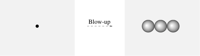
Figure 2: Maximal partial resolution of ${\mathchoice{\mbox{\bbbfont C}}{\mbox{\bbbfont C}}{\mbox{\smallbbbfont C}}{\mbox{\tinybbbfont C}}}^{9}/({\mathchoice{\mbox{\bbbfont Z}}{\mbox{\bbbfont Z}}{\mbox{\smallbbbfont Z}}{\mbox{\tinybbbfont Z}}}_{4}\times{\mathchoice{\mbox{\bbbfont Z}}{\mbox{\bbbfont Z}}{\mbox{\smallbbbfont Z}}{\mbox{\tinybbbfont Z}}}_{4})$ with $K=0$.

Let us now analyze the critical point set of $W$. Finding B we determine from (17) that

$$W=a_{1}x_{1}^{4}x_{10}^{3}x_{11}^{2}x_{12}+a_{2}x_{2}^{4}x_{10}x_{11}^{2}x_{12}^{3}+a_{3}x_{3}^{2}+a_{4}x_{4}^{4}+a_{5}x_{5}^{4}+a_{6}x_{6}^{2}+a_{7}x_{7}^{4}+a_{8}x_{8}^{4}+a_{9}x_{9}^{2}+\ldots$$ (32)

In total there are 87 points in B but we need only consider the above terms with nonzero $a_{1},\ldots,a_{9}$ for a sufficiently generic $W$.

Consider the maximal triangulation. This includes all three points $\alpha_{10},\alpha_{11},\alpha_{12}$. Since $N=12$ we need to remove the set $F_{\Delta}$ given by (10) from ${\mathchoice{\mbox{\bbbfont C}}{\mbox{\bbbfont C}}{\mbox{\smallbbbfont C}}{\mbox{\tinybbbfont C}}}_{12}$. This amounts in imposing $x_{2}x_{11}x_{12}\neq 0$ or $x_{1}x_{2}x_{12}\neq 0$ or $x_{1}x_{2}x_{10}\neq 0$ or $x_{1}x_{10}x_{11}\neq 0$. We also wish to impose $\partial W/\partial x_{i}=0$ for $i=1,\ldots,12$. It is straight-forward to show that these conditions require

 

$${x_{3}=x_{4}=x_{5}=x_{6}=x_{7}}$$

  (33)

and that $x_{10}$ and $x_{12}$ cannot both be zero simultaneously. As $N-n=3$ we have three ${\mathchoice{\mbox{\bbbfont C}}{\mbox{\bbbfont C}}{\mbox{\smallbbbfont C}}{\mbox{\tinybbbfont C}}}^{*}$ actions to divide this subspace of ${\mathchoice{\mbox{\bbbfont C}}{\mbox{\bbbfont C}}{\mbox{\smallbbbfont C}}{\mbox{\tinybbbfont C}}}^{12}$ by. Two may be used to fix $x_{1}$ and $x_{2}$ to specific values. The other ${\mathchoice{\mbox{\bbbfont C}}{\mbox{\bbbfont C}}{\mbox{\smallbbbfont C}}{\mbox{\tinybbbfont C}}}^{*}$ may be used to turn $x_{10}$ and $x_{12}$ into homogeneous coordinates parametrizing ${\mathchoice{\mbox{\bbbfont P}}{\mbox{\bbbfont P}}{\mbox{\smallbbbfont P}}{\mbox{\tinybbbfont P}}}^{1}$. The vacuum is thus ${\mathchoice{\mbox{\bbbfont P}}{\mbox{\bbbfont P}}{\mbox{\smallbbbfont P}}{\mbox{\tinybbbfont P}}}^{1}$. One may also determine the superpotential in this vacuum to show that we have a Landau-Ginzburg theory fibered over this ${\mathchoice{\mbox{\bbbfont P}}{\mbox{\bbbfont P}}{\mbox{\smallbbbfont P}}{\mbox{\tinybbbfont P}}}^{1}$ to obtain the familiar hybrid-type models of [1, 3]. One may also show that the fiber has a ${\mathchoice{\mbox{\bbbfont Z}}{\mbox{\bbbfont Z}}{\mbox{\smallbbbfont Z}}{\mbox{\tinybbbfont Z}}}_{4}$-quotient singularity at the zero section.

In terms of the ambient toric variety $V_{\Delta}$, what we have just described in the previous paragraph is the ${\mathchoice{\mbox{\bbbfont P}}{\mbox{\bbbfont P}}{\mbox{\smallbbbfont P}}{\mbox{\tinybbbfont P}}}^{1}$ that appears in the middle of the chain of three ${\mathchoice{\mbox{\bbbfont P}}{\mbox{\bbbfont P}}{\mbox{\smallbbbfont P}}{\mbox{\tinybbbfont P}}}^{1}$’s on the right in figure 2. Thus although $V_{\Delta}$ appears to have three degrees of freedom for the Kähler form — giving the three independent sizes of the three ${\mathchoice{\mbox{\bbbfont P}}{\mbox{\bbbfont P}}{\mbox{\smallbbbfont P}}{\mbox{\tinybbbfont P}}}^{1}$’s, only one makes it down to $X$, the critical point set of $W$. Therefore $X$ only has one Kähler-type deformation. Sometimes additional modes appear in the fibre for these hybrid models but in this case the Landau-Ginzburg fibre contains no twist fields with the correct charges to be considered a (1,1)-form. We will therefore assert that $h^{1,1}(X)=1$. Thus we are in agreement with the assertions concerning the mirror space at the start of this section.

Analyzing the other possible triangulations we find that we reproduce one of the two phases we know about — either the Landau-Ginzburg orbifold in ${\mathchoice{\mbox{\bbbfont C}}{\mbox{\bbbfont C}}{\mbox{\smallbbbfont C}}{\mbox{\tinybbbfont C}}}^{9}/({\mathchoice{\mbox{\bbbfont Z}}{\mbox{\bbbfont Z}}{\mbox{\smallbbbfont Z}}{\mbox{\tinybbbfont Z}}}_{4}\times{\mathchoice{\mbox{\bbbfont Z}}{\mbox{\bbbfont Z}}{\mbox{\smallbbbfont Z}}{\mbox{\tinybbbfont Z}}}_{4})$ or the hybrid model over ${\mathchoice{\mbox{\bbbfont P}}{\mbox{\bbbfont P}}{\mbox{\smallbbbfont P}}{\mbox{\tinybbbfont P}}}^{1}$. The points $\alpha_{10}$ and $\alpha_{12}$ may be ignored when considering $X$. Thus we have constructed a model with a non-trivial phase diagram — there are 2 phases — but neither is a Calabi-Yau space.

In general there is a homomorphism:

$$\kappa:H^{1,1}(V_{\Delta})\to H^{1,1}(X).$$ (34)

In general however $\kappa$ is neither injective nor surjective. The example in this section shows a failure of injectivity since $h^{1,1}(V_{\Delta})=3$ and $h^{1,1}(X)=1$. In the more simple case of $\langle\mu,\nu\rangle=1$ it was shown in [16] that the kernel of $\kappa$ was described by points in the interior of co-dimension one faces of the convex hull of A. In the case described in this section we see that such a simple criterion cannot be used — all the points $\alpha_{10},\alpha_{11},\alpha_{12}$ lie in a co-dimension 7 face and yet $\alpha_{10}$ and $\alpha_{12}$ contribute to the kernel and $\alpha_{11}$ survives through to $H^{1,1}(X)$. At this point in we know of no simple method of determining the image of $\kappa$ except to explicitly calculate the critical point set of $W$ on a case by case basis.

Let us conclude this section by discussing the short-comings of analyzing this model in terms of the “generalized Calabi-Yau manifolds” of [5]. The ${\mathchoice{\mbox{\bbbfont Z}}{\mbox{\bbbfont Z}}{\mbox{\smallbbbfont Z}}{\mbox{\tinybbbfont Z}}}_{4}$ singularity in ${\mathchoice{\mbox{\bbbfont C}}{\mbox{\bbbfont C}}{\mbox{\smallbbbfont C}}{\mbox{\tinybbbfont C}}}^{9}$ generated by $g_{1}$ of (29) may be partially resolved by a line bundle over the weighted projective space ${\mathchoice{\mbox{\bbbfont P}}{\mbox{\bbbfont P}}{\mbox{\smallbbbfont P}}{\mbox{\tinybbbfont P}}}^{8}_{\{1,1,2,1,1,2,1,1,2\}}$. The resultant space has $K<0$. The “generalized Calabi-Yau manifold”, $R$, would be identified as the hypersurface in this weighted projective space given by the vanishing of (32) with $x_{1},\ldots,x_{9}$ taken to be the quasi-homogeneous coordinates and $x_{10}=x_{11}=x_{12}=1$. The ${\mathchoice{\mbox{\bbbfont Z}}{\mbox{\bbbfont Z}}{\mbox{\smallbbbfont Z}}{\mbox{\tinybbbfont Z}}}_{4}$-action of $g_{2}$ acts on $R$ to induce ${\mathchoice{\mbox{\bbbfont Z}}{\mbox{\bbbfont Z}}{\mbox{\smallbbbfont Z}}{\mbox{\tinybbbfont Z}}}_{4}$-quotient singularities over some subspace of codimension two. These latter singularities are not terminal and may be resolved without adding anything further to $K$. In fact, resolving these latter singularities may be achieved by introducing the points $\alpha_{10},\alpha_{11},\alpha_{12}$ into the toric fan.

It is easy to see that something similar will happen in general. That is, any $K=0$ toric resolutions we may perform in $V_{\Delta}$ may also be performed after blowing up any terminal singularities in $V_{\Delta}$. It follows that the points in the interior of the convex hull of A may be counted by analyzing singularities which may be locally resolved with $K=0$ in $R$. (Note that this is a rather inefficient way of proceeding in our picture — one may as well just analyze the singularities in $V_{\Delta}$ without any destroying the $K=0$ condition.) This observation sheds light on a conjecture in [27] that $h^{1,1}(X)$ could be determined by counting the contribution to $h^{1,1}$ of any resolutions of singularities within the $R$. We see now that this will count $h^{1,1}(V_{\Delta})$ which is, in general, not equal to $h^{1,1}(X)$. Thus this conjecture is false. In the example above, counting this way would imply that $h^{1,1}(X)=3$.

With regards to determining $h^{1,1}(X)$, it appears hard to save the construction of [6] from a similar fate. The problem is that the divisors associated with $\alpha_{10}$, $\alpha_{11}$ and $\alpha_{12}$ appear on equal footing in $R$. Thus unless some unsymmetric rules are devised for resolving canonical singularities in superspace one cannot obtain the correct answer $h^{1,1}(X)=1$.

3.4 A Case with $X=\hbox{\bigbbbfont P}^{3}$

One might be led to suspect the following to be the general picture for the geometric interpretation of an $N$=2 superconformal field theory. Either $X$ is a Calabi-Yau space and the string is free to move within $X$ and there are no massless modes normal to $X$, or $X$ is a space of dimension $<d$ in which the string is free to move and there are massless modes governed by some superpotential normal to $X$ inside some bigger ambient space $V_{\Delta}$ containing $X$. We now show an example (which also appeared in [1]) which is an exception to this.

Consider the following point set for A :

 

$${\alpha_{1}}$$

  (35)

Thus $\mu=(0,0,0,0,0,0,0,1,1,1,1)$. One can also determine B with a little effort and find $\nu=(0,0,0,0,0,0,0,1,1,1,1)$. Thus $d=3$ again. The superpotential $W$ may be written

$$W=x_{9}G_{1}+x_{10}G_{2}+x_{11}G_{3}+x_{12}G_{4},$$ (36)

where the $G_{k}$ are generic homogeneous polynomials of total degree two in $x_{1},\ldots,x_{8}$.

There are two triangulations of the point set A. The first consists of taking 8 simplices each of which has $\alpha_{9},\ldots,\alpha_{12}$ as 4 of its vertices with the other 7 vertices taken from the set $\{\alpha_{1},\ldots,\alpha_{8}\}$. In terms of $F_{\Delta}$ this amounts to removing the point $x_{1}=\ldots=x_{8}=0$ from consideration. Restricting to the critical point set of $W$ forces $x_{9}=\ldots=x_{12}=0$ and $G_{1}=\ldots=G_{4}=0$. Dividing out by the single required ${\mathchoice{\mbox{\bbbfont C}}{\mbox{\bbbfont C}}{\mbox{\smallbbbfont C}}{\mbox{\tinybbbfont C}}}^{*}$-action forms ${\mathchoice{\mbox{\bbbfont P}}{\mbox{\bbbfont P}}{\mbox{\smallbbbfont P}}{\mbox{\tinybbbfont P}}}^{7}$ with homogeneous coordinates $x_{1},\ldots,x_{8}$. Thus $X$ is the intersection of 4 quadric equations $G_{k}=0$ in ${\mathchoice{\mbox{\bbbfont P}}{\mbox{\bbbfont P}}{\mbox{\smallbbbfont P}}{\mbox{\tinybbbfont P}}}^{7}$. This is a known Calabi-Yau space dating back to [22].

The other triangulation consists of 4 simplices with 8 vertices given by $\alpha_{1},\ldots,\alpha_{8}$ with the other 3 taken from the set $\{\alpha_{9},\ldots,\alpha_{12}\}$. This amounts to removing $x_{9}=\ldots=x_{12}=0$ from consideration. Restricting to the critical point set of $W$ forces $x_{1}=\ldots=x_{8}=0$. Now the ${\mathchoice{\mbox{\bbbfont C}}{\mbox{\bbbfont C}}{\mbox{\smallbbbfont C}}{\mbox{\tinybbbfont C}}}^{*}$-action may be used to form ${\mathchoice{\mbox{\bbbfont P}}{\mbox{\bbbfont P}}{\mbox{\smallbbbfont P}}{\mbox{\tinybbbfont P}}}^{3}$ with homogeneous coordinates $x_{9},\ldots,x_{12}$. Thus $X$ in this phase is ${\mathchoice{\mbox{\bbbfont P}}{\mbox{\bbbfont P}}{\mbox{\smallbbbfont P}}{\mbox{\tinybbbfont P}}}^{3}$.

Our phase diagram consists of two phases — both of which have the dimension of $X$ equal to $d$. One phase is a Calabi-Yau manifold with $h^{1,1}=1$ and $h^{2,1}=65$ which we understand. The other phase is ${\mathchoice{\mbox{\bbbfont P}}{\mbox{\bbbfont P}}{\mbox{\smallbbbfont P}}{\mbox{\tinybbbfont P}}}^{3}$. The reader might be alarmed at the appearance of the latter since ${\mathchoice{\mbox{\bbbfont P}}{\mbox{\bbbfont P}}{\mbox{\smallbbbfont P}}{\mbox{\tinybbbfont P}}}^{3}$ is not a Calabi-Yau space and lacks a nonvanishing holomorphic 3-form for example. The resolution is as follows. Although we have correctly identified the vacuum of the field theory as $X$ we have to be a little careful in declaring it to be the effective target space of a conformal field theory. Let us consider the variables $\alpha_{1},\ldots,\alpha_{8}$ which we forced to zero. The superpotential is quadratic in these variables so we certainly haven’t missed any massless degrees of freedom (which would only add to our troubles by increasing $d$ anyway). The point is that there is actually a ${\mathchoice{\mbox{\bbbfont Z}}{\mbox{\bbbfont Z}}{\mbox{\smallbbbfont Z}}{\mbox{\tinybbbfont Z}}}_{2}$-quotient singularity coming from the identification of homogeneous coordinates in $V_{\Delta}$ to affine ones. Thus we have a fibration of a Landau-Ginzburg orbifold theory over ${\mathchoice{\mbox{\bbbfont P}}{\mbox{\bbbfont P}}{\mbox{\smallbbbfont P}}{\mbox{\tinybbbfont P}}}^{3}$ which may appear trivial in that the superpotential is quadratic but we may expect twist fields is add to our spectrum. In particular we expect to have an analog to a Calabi-Yau $H^{3,0}$ mode (i.e. a field of charge (3,0) under the $U(1)_{L}\times U(1)_{R}$ of the superconformal algebra) coming from such twisted sectors. Of course, such a mode cannot be given a literal geometric interpretation in terms of a (3,0)-form.

It is interesting also to ask how literally we can take this ${\mathchoice{\mbox{\bbbfont P}}{\mbox{\bbbfont P}}{\mbox{\smallbbbfont P}}{\mbox{\tinybbbfont P}}}^{3}$ to be a target space for the conformal field theory. To find the actual size of truly conformally invariant $\sigma$-model target space one needs to solve the Picard-Fuchs system as described in [7]. We will not present the details here since they are rather lengthy but we may quickly summarize as follows. One solves equations (42) of [7] where the “$\beta$” vector of this system is set equal to $-\nu$. (One could then count rational curves on this Calabi-Yau space if one so desired.) The complexified Kähler form $B+iJ$ of the Calabi-Yau phase can then be analytically continued into ${\mathchoice{\mbox{\bbbfont P}}{\mbox{\bbbfont P}}{\mbox{\smallbbbfont P}}{\mbox{\tinybbbfont P}}}^{3}$ phase (which is most easily done by the method of [28]). Taking $z$ to be the local coordinate on the moduli space where $z=0$ corresponds to the limit point in the ${\mathchoice{\mbox{\bbbfont P}}{\mbox{\bbbfont P}}{\mbox{\smallbbbfont P}}{\mbox{\tinybbbfont P}}}^{3}$ phase we obtain

$$B+iJ=-{\textstyle\frac{1}{2}}-\frac{3\pi i}{2\log(z)}+O(\log(z)^{-2}).$$ (37)

Thus $J\geq 0$ in the region near the limit point $|z|\ll 1$. The effective size of target space is very small as $|z|\to 0$. In other words, the effect of integrating out the massive modes in the linear $\sigma$-model of [1] has caused an infinite renormalization of the “$r$” parameter (unlike what is believed to happen for the Calabi-Yau phase).

To summarize we see that the phase picture can produce phases with dimension equal to $d$ which do not correspond to Calabi-Yau non-linear $\sigma$-models. To understand these phases more completely will require a better understanding of the hybrid models.

4 Conclusions

Geometrical methods have proven themselves to be a powerful conceptual and calculational tool in understanding the physical content of certain conformal theories and their associated string models. As such, it is a worthwhile task to gain as complete an understanding as possible of the geometrical status of conformal field theories, especially for the case of $N=2$ worldsheet supersymmetry relevant for spacetime supersymmetric string models. The phase structure of such $N=2$ models, as found in [1, 3], goes a long way towards capturing the full geometric content of these theories, and, in particular, certainly provides the correct framework for discussing mirror symmetry. In this paper we have used this phase structure analysis to address certain previously puzzling issues regarding the geometrical content of certain theories. In particular, at first sight mirror symmetry seems to come upon the puzzle regarding the identity of the mirror of a rigid manifold. We have seen, though, that this appears to be a puzzle only because the question itself is not phrased in the correct context. That is, mirror symmetry tells us that certain a priori distinct pairs of families of conformal theories actually are composed of isomorphic members. When the phase structure of each family in such a pair contains a Calabi-Yau $\sigma$-model region, then these Calabi-Yau’s form a mirror pair. However, in certain cases, at least one of the families does not have a Calabi-Yau $\sigma$-model region. In such cases mirror symmetry will simply not yield a mirror pair of Calabi-Yau manifolds. A family which has a rigid Calabi-Yau phase, as we have seen, provides one such example — the mirror family does not have a Calabi-Yau region. Thus the absence of a Kähler form for the mirror is not an issue. The mirror moduli space has no Calabi-Yau phase and hence does not require a Kähler form. The previous puzzle disappears, therefore, when the question is phrased in the correct context.

Beyond the rigid case, we have also seen that even when there is a conformal mode that can play the part of a Kähler form, there need not be a Calabi-Yau phase on which it can realize this potential. So, whereas in the previous problem we resolved the issue of a “Calabi-Yau in search of a Kähler form” here we have “a Kähler form in search of a Calabi-Yau”. We have established that there are examples in which there simply is no Calabi-Yau to be found.

It is worth noting that the map $\kappa$ in (34) is neither injective or surjective. We saw the effect on this map not being injective in section 3.3. The failure of surjectivity shows that some (1,1)-forms on $X$ do not come from the toric ambient space $V_{\Delta}$. In the case of models of the form discussed in section 3.1 it is still possible to count the number $h^{1,1}(X)$ because of the properties of hypersurfaces [19, 16]. In the cases considered here however we deal with more general complete intersections. The problem of counting $h^{1,1}(X)$ in this context is the mirror of the problem of counting $h^{2,1}$ for the mirror model. The analogue of the fact that $\kappa$ is not an isomorphism is the fact that deforming the polynomial giving the superpotential is not the same as deformation the complex structure. It would be interesting to see if methods along the lines of [29] could be applied in this context to determine the Hodge numbers of $X$.

An interesting question, to which we do not know the answer, is whether there are examples in which neither family in a mirror pair has a Calabi-Yau region. Such an example would establish that there are $N=2,c=3d$ conformal theories which are not interpretable in terms of Calabi-Yau compactifications (or analytic continuations thereof). To answer this question is difficult because of the failure of the surjectivity of $\kappa$. One may find mirror pairs of orbifolds of the Gepner model, ${\bf 1}^{9}$, for which neither has an obvious Calabi-Yau interpretation. An example with $h^{1,1}$ and $h^{2,1}$ equal to 4 and 40 was mentioned in [23]. This is a good candidate for a situation where neither of the mirror partners have a Calabi-Yau phase (despite the assertions of [23]). Unfortunately if $X$ is the model with $h^{1,1}=4$ then the image of $\kappa$ is trivial, i.e., none of the (1,1)-forms come from $V_{\Delta}$. Because of this the methods of this paper cannot be used to draw any conclusions regarding the lack of Calabi-Yau phase for this example.

Note Added

The mirror of the example of section 3.4 was studied in [30] where it was discovered that there is an extra ${\mathchoice{\mbox{\bbbfont Z}}{\mbox{\bbbfont Z}}{\mbox{\smallbbbfont Z}}{\mbox{\tinybbbfont Z}}}_{2}$ symmetry in the moduli space. This should act on the moduli space in section 3.4 to identify the two phases with each other. This may be viewed as a new kind of $R\leftrightarrow 1/R$ symmetry.

References

- [1] E. Witten, Phases of Theories in Two Dimensions, Nucl. Phys. B403 (1993) 159–222.
- [2] P. S. Aspinwall, B. R. Greene, and D. R. Morrison, Multiple Mirror Manifolds and Topology Change in String Theory, Phys. Lett. 303B (1993) 249–259.
- [3] P. S. Aspinwall, B. R. Greene, and D. R. Morrison, Calabi-Yau Moduli Space, Mirror Manifolds and Spacetime Topology Change in String Theory, Nucl. Phys. B416 (1994) 414–480.
- [4] P. Candelas, E. Derrick, and L. Parkes, Generalized Calabi-Yau Manifolds and the Mirror of a Rigid Manifold, Nucl.Phys. B407 (1993) 115–154.
- [5] R. Schimmrigk, Critical Superstring Vacua from Noncritical Manifolds: A Novel Framework for String Compactification, Phys. Rev. Lett. 70 (1993) 3688–3691.
- [6] S. Sethi, Supermanifolds, Rigid Manifolds and Mirror Symmetry, Nucl. Phys. B430 (1994) 31–50.
- [7] P. S. Aspinwall, B. R. Greene, and D. R. Morrison, Measuring Small Distances in Sigma Models, Nucl. Phys. B420 (1994) 184–242.
- [8] F. C. Kirwan, Cohomology of Quotients in Symplectic and Algebraic Geometry, Number 31 in Mathematical Notes, Princeton University Press, Princeton, 1984.
- [9] L. Ness, A Stratification of the Null Cone Via the Moment Map, Amer. J. Math. 106 (1984) 1281–3129.
- [10] A. D’Adda, P. D. Vecchia, and M. Lüscher, Confinement and Chiral Symmetry Breaking in Models with Quarks, Nucl. Phys. B152 (1979) 125–144.
- [11] P. Griffiths and J. Harris, Principles of Algebraic Geometry, Wiley-Interscience, 1978.
- [12] D. A. Cox, The Homogeneous Coordinate Ring of a Toric Variety, Amherst 1992 preprint, alg-geom/9210008, to appear in J. Algebraic Geom.
- [13] M. Reid, Minimal models of canonical 3-folds, in S. Iitaka, editor, “Algebraic Varieties and Analytic Varieties”, volume 1 of Adv. Studies in Pure Math., pages 131–180, Kinokuniya, Tokyo, 1983.
- [14] C. Vafa and N. Warner, Catastrophes and the Classification of Conformal Theories, Phys. Lett 218B (1989) 51–58.
- [15] V. V. Batyrev and L. A. Borisov, Dual Cones and Mirror Symmetry for Generalized Calabi-Yau Manifolds, Essen and Michigan 1994 preprint, alg-geom/9402002.
- [16] P. S. Aspinwall, B. R. Greene, and D. R. Morrison, The Monomial-Divisor Mirror Map, Internat. Math. Res. Notices 1993 319–338.
- [17] S. Katz and D. Morrison, The Multinomial-Divisor Mirror Map, to appear.
- [18] B. R. Greene and M. R. Plesser, Duality in Calabi-Yau Moduli Space, Nucl. Phys. B338 (1990) 15–37.
- [19] V. V. Batyrev, Dual Polyhedra and Mirror Symmetry for Calabi-Yau Hypersurfaces in Toric Varieties, J. Alg. Geom. 3 (1994) 493–535.
- [20] L. Borisov, Towards the Mirror Symmetry for Calabi-Yau Complete Intersections in Gorenstein Toric Fano Varieties, Michigan 1993 preprint, alg-geom/9310001.
- [21] M. Reid, Young Person’s Guide to Canonical Singularities, Proc. Symp. Pure Math. 46 (1987) 345–414.
- [22] P. Candelas, G. Horowitz, A. Strominger, and E. Witten, Vacuum Configuration for Superstrings, Nucl. Phys. B258 (1985) 46–74.
- [23] P. S. Aspinwall and C. A. Lütken, Geometry of Mirror Manifolds, Nucl. Phys. B353 (1991) 427–461.
- [24] D. Gepner, Exactly Solvable String Compactifications on Manifolds of Holonomy, Phys. Lett. 199B (1987) 380–388.
- [25] P. S. Aspinwall and D. R. Morrison, String Theory on K3 Surfaces, Duke and IAS 1994 preprint DUK-TH-94-68, IASSNS-HEP-94/23, hep-th/9404151, to appear in “Essays on Mirror Manifolds 2”.
- [26] P. Berglund, Dimensionally Reduced Landau-Ginzburg Orbifolds with Discrete Torsion, Phys. Lett. 319B (1993) 117–124.
- [27] R. Schimmrigk, Mirror Symmetry and String Vacua From a Special Class of Fano Varieties, Bonn 1994 preprint BONN-TH-94-007, hep-th/9405086.
- [28] P. S. Aspinwall, Minimum Distances in Non-Trivial String Target Spaces, Nucl. Phys. B431 (1994) 78–96.
- [29] P. Green and T. Hübsch, Polynomial Deformations and Cohomology of Calabi-Yau Manifolds, Commun. Math. Phys. 113 (1987) 505–528.
- [30] P. Berglund et al., Periods for Calabi-Yau and Landau-Ginzburg Vacua, Nucl. Phys. B419 (1994) 352–403.