RU-94-72
Large $N$ Gauge Theory – Expansions and Transitions

Abstract

We use solvable two-dimensional gauge theories to illustrate the issues in relating large $N$ gauge theory to string theory. We also give an introduction to recent mathematical work which allows constructing master fields for higher dimensional large $N$ theories. We illustrate this with a new derivation of the Hopf equation governing the evolution of the spectral density in matrix quantum mechanics.

Based on lectures given at the 1994 Trieste Spring School on String Theory, Gauge Theory and Quantum Gravity.

1 Introduction

The idea that QCD can be reformulated as some sort of string theory refuses to die. If we allow ourselves a sufficiently liberal definition of ‘string theory’ – I will take this to be ‘a theory of embeddings of two-dimensional manifolds into space-time with an action local both on the world-sheet and in space-time,’ allowing other degrees of freedom as well and noting that the possible theories have not yet been classified – we should agree that the idea has not been disproven. Nevertheless it has been difficult to make progress with it.

In these lectures I will describe some of the work which has been done in the last two years on two dimensional gauge theory. Although this is drastically simpler than the four dimensional theory and can only illustrate a few qualitative features common to both cases, some important ideas have come out of this work, which suggest new lines to pursue in four dimensions.

A good starting point for discussing ‘QCD string’ is the strong coupling expansion, which I will review very briefly. (See [31]; the large $N$ case was discussed in detail by V. Kazakov and I. Kostov at the 1993 Trieste Spring School [35, 37].) We write the path integral

$$Z=\int DA~{}e^{-N\beta S_{YM}[A]},$$ (1)

expand in a power series in $\beta=1/g^{2}$, integrate termwise, and sum. To do this, it is necessary to be able to make sense of the functional measure $DA$ without benefit of the Boltzmann weight, and so far the only way known to do this in $D>2$ is to latticize the theory. We thus use the Wilson action $S[U]=\sum_{P}{\rm tr\ }U(P)+U^{+}(P)$ and link integrals such as $\int dU(L)~{}U(L){}^{i_{1}}_{j_{1}}U(L)^{+}{}^{i_{2}}_{j_{2}}={1\over N}\delta{}^{i_{1}}_{j_{2}}\delta{}^{i_{2}}_{j_{1}}$ to evaluate the $O(\beta^{n})$ term as a sum over diagrams with $n$ plaquettes glued together in a continuous and ‘surface-like’ way. This expansion has a finite radius of convergence (because the number of diagrams only grows exponentially in $n$) and clearly produces area law behavior for Wilson loops at small $\beta$.

At large $N$, one can interpret the rules for building diagrams in a way which makes a diagram with weight $N^{2-2g}$ into a continuous two-dimensional manifold of genus $g$. Basically, this is because each link integral, contributing an edge to the diagram, produces $1/N$; the usual large $N$ coupling dependence gives each plaquette an $N$, while each vertex comes with a sum over an independent index, giving $N$. (The roles of vertices and faces are switched from the weak coupling expansion.) The main subtlety is dealing with link integrals such as

$$\int dU~{}U{}^{i_{1}}_{j_{1}}U{}^{i_{2}}_{j_{2}}U^{+}{}^{i_{3}}_{j_{3}}U^{+}{}^{i_{4}}_{j_{4}}={1\over N^{2}}\delta{}^{i_{1}}_{j_{3}}\delta{}^{i_{3}}_{j_{1}}\delta{}^{i_{2}}_{j_{4}}\delta{}^{i_{4}}_{j_{2}}$$ (2)

$$\qquad-{1\over N^{3}}\delta{}^{i_{1}}_{j_{3}}\delta{}^{i_{3}}_{j_{2}}\delta{}^{i_{2}}_{j_{4}}\delta{}^{i_{4}}_{j_{1}}\qquad$$

$$\qquad+3\leftrightarrow 4.\qquad$$

The subleading terms in this expression can contribute to a diagram with overall weight $N^{2}$, and thus we must interpret an appearance of this term as a geometric object which can be glued to the rest of the surface to form a sphere. This will work if we call it a ‘disk’ with four edges and zero area, as in figure 1 – the geometrical $N$ counting is $N^{1-4}$ which agrees with the result from the integral. The minus sign is to be interpreted as a weight associated with this feature. Higher ‘saddles’ with more edges also appear in the full expansion.

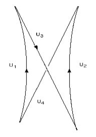
Figure 1: A world-sheet ‘saddle’ associated with terms like (3). Every edge is embedded in the same lattice link.

This already looks pretty close to the definition of ‘string theory’ I started with and thus the project of finding a world-sheet action associated with some continuum limit of this to get a ‘gauge string’ seems very well motivated. Already on this qualitative level, many differences with fundamental string theory are apparent. Perhaps the most striking is that the world-sheets are continuously embedded in the target space: this is incompatible with a world-sheet action $\int d^{2}\sigma(\partial X)^{2}$ and not easy to describe with a unitary world-sheet theory, but on the other hand it may explain why in QCD string theory (unlike the fundamental string) we can define correlation functions of operators local in target space. [16]

A serious objection can be raised to starting from a strong coupling expansion: to take the continuum limit of the theory, we must take $g\rightarrow 0$ and the lattice spacing to zero as prescribed by the RG, and surely it is unrealistic to hope that the expansion will have infinite radius of convergence. One response to this objection is to argue that our string theory will agree with gauge theory only at long distances, and that this is an acceptable limitation. I disagree with this response. On theoretical grounds, if this is what we want, we can simply use the effective long-distance theory defined by Polchinski and Strominger [45], because no structure specific to the underlying gauge theory survives in the long distance limit. On practical grounds, what is lacking is a precise calculational technique which works for intermediate scales, interpolating between the known short and long distance behaviors, and if we do not get the short distance behavior right, it is not likely we will get the interpolation right.

Thus we either must abandon the strong coupling expansion or be optimists and look for a version for which summation and analytic continuation produces the correct result as $g\rightarrow 0$. If we can represent it as a string theory, an appropriate treatment of that theory may well do the analytic continuation for us. A solid result which speaks against this possibility is the roughening transition – I refer to [36] for a discussion of this but note only that the real cause of this was the lattice discretization, and that a continuum string theory will not have it.

The most direct and explicit version of this idea would be to develop a continuum strong coupling expansion. In $D>2$ we need a regulator, but in principle any continuum regulator which allows us to make sense of $\int DA$ without the Boltzmann weight might be used. Although it would depend on the choice of regulator, it would surely be a more natural expansion than the lattice expansion, and conceivably free of spurious phase transitions. This is one way to make the concept of ‘QCD string’ precise. We will make contact with my original definition if we can associate terms with surfaces, if the weight for each surface is determined by local rules, and if we can reproduce the weight with a local world-sheet action.

Such a string theory has been developed by D. Gross and W. Taylor for two-dimensional Yang-Mills theory. [24] They gave local rules for the weights and it can also be defined by a continuum world-sheet action, as described by G. Moore in his lectures. [10, 28]

There is no obvious reason that a similar expansion for a regulated higher dimensional theory could not exist. The regulator would have to act solely on the measure and preserve gauge invariance – thus the likely candidates are stochastic regularizations. [2, 11] I feel this possibility is the most important lesson to be drawn from the work.

Will it be QCD? In other words, will the $g\rightarrow 0$ limit reproduce weak coupling physics? It is difficult to get at this question using the expansion itself – a priori, even if it converges, we will need more and more terms to get a result as $g\rightarrow 0$. We expect the world-sheet theory to be strongly coupled at short distances. [16] Conceivably, we might end up with an exact string reformulation of QCD, in which (say) the one-gluon exchange graph is uncalculable.

A better approach is to use other methods to study the analyticity of the partition function. Combining this information with the known finite radius of convergence of the strong coupling expansion will show its validity. Clearly we should start by answering this question in the two-dimensional case, which we can solve exactly.

2 Two dimensional Yang-Mills theory

There are many ways to solve the two dimensional theory, and it is worth doing it in more than one way, first because the techniques come up elsewhere, and second because it is conceivable that one of them will provide insight for higher dimensions.

YM₂ is very easy to work with, first because the action $\int d^{2}x~{}{\rm tr\ }F^{2}$ only depends on the volume form, and second, as pointed out long ago by A. Migdal, there is a lattice definition which is equivalent to the continuum theory. The Boltzmann weight (‘heat kernel action’) $Z(U,A)$ for a plaquette of area $A$ and boundary holonomy $U$ is just the continuum YM₂ path integral on the plaquette. Let the plaquette be the disk with coordinates $(r,\theta)$ and $\pi r^{2}\leq A$; the $A$ dependence can be determined as Hamiltonian evolution with $r$ as time. Fixing $A_{r}=0$ gauge and imposing Gauss’ law, the wave function depends only on the holonomy $U=\exp i\int d\theta_{0}^{2\pi}A_{\theta}$. The Hamiltonian is

$$H={g^{2}\over 2N}{\rm tr\ }\left(U{\partial\over\partial U}\right)^{2}\equiv{g^{2}\over 2N}\sum_{a}E^{a}E^{a}.$$ (4)

This is the only appearance of $g^{2}$ and from now on we normally choose units of length in which $g^{2}=1$. $E^{a}={\rm tr\ }t^{a}Ud/dU$ generates left rotations of $U$ and represents the Lie algebra $u(N)$. Thus acting on a wave function which could be any matrix element of an irreducible representation $R$, $\psi(U)=D^{(R)}_{i\bar{j}}(U)$, $H=C_{2}(R)$, the second Casimir (normalized so that $C_{2}({\lower 1.3pt\vbox{\hrule height=0.4pt\hbox{\vrule width=0.4pt\vbox{\hbox to8.0pt{\vbox to8.0pt{\vfil}\hfil}}\vrule width=0.4pt}\hrule height=0.4pt}\hskip-0.2pt})=N$). Gauge invariant wave functions $\psi(U)=\psi(gUg^{-1})$ are class functions, which can be expanded in characters $\chi_{R}(U)={\rm tr\ }D^{(R)}(U)$. Let $\chi_{R}(U)$ be the character of the irreducible representation $R$ with $\chi_{R}(1)=\dim R$; the measure $\int DU$ is normalized so $\int DU~{}\chi_{R}(U)\chi_{S}(U^{+})=\delta_{RS}$. These results combine to determine the path integral $Z(U_{1},U_{2};A)$ on a cylinder of area $A$ and boundary holonomies $U_{1}$ and $U_{2}$: the final ingredient is the boundary condition $Z(U_{1},U_{2};0)=\delta(U_{1},U_{2})=\sum_{R}\chi_{R}(U_{1})\chi_{R}(U_{2}^{+})$ on class functions, so

$$Z(U_{1},U_{2};A)=\sum_{R\in\hat{G}}\chi_{R}(U_{1})\chi_{R}(U_{2}^{+})e^{-{A\over 2N}C_{2}(R)}.$$ (5)

($\hat{G}$ is the set of irreducible representations of $G$). We can then set $U_{2}=1$, the holonomy for a zero area plaquette, to get $Z(U;A)$. By writing $\chi_{R}(UV)={\rm tr\ }D^{(R)}(U)D^{(R)}(V)$ and using $\int dUD^{(R)}_{i\bar{j}}(U)D^{(S)}_{k\bar{l}}(U^{+})={1\over\dim R}\delta_{RS}\delta_{i\bar{l}}\delta_{k\bar{j}}$ one can check the ‘self-reproducing’ property

$$\int dVZ(UV^{-1};A_{1})Z(VW;A_{2})$$

$$\qquad=Z(UW;A_{1}+A_{2}).$$ (6)

This implies that the lattice integral is invariant under subdividing the discretization and thus this is equivalent to the continuum limit.

Perhaps the simplest result is the calculation of the partition function on a Riemann surface due to A. Migdal and B. Rusakov. [48] We can form a genus ${\rm g}$ surface by identifying the edges of a $4{\rm g}$-gon as $A_{1}B_{1}A_{1}^{-1}B_{1}^{-1}A_{2}B_{2}A_{2}^{-1}B_{2}^{-1}\ldots$ and it is an entertaining calculation to check that

$$Z_{\rm g}(A)=\sum_{R\in\hat{G}}(\dim R)^{2-2{\rm g}}~{}e^{-{A\over 2N}C_{2}(R)}.$$ (7)

We specialize this to the group $U(N)$ to study the large $N$ limit. This choice turns out a bit simpler than $SU(N)$ but one might worry that we are introducing extra degrees of freedom which will confuse matters. The $U(1)$ factor is a gauge theory with gauge coupling $g^{2}/N\rightarrow 0$ in the limit, so perturbatively this completely decouples. However, $U(N)$ is not a direct product but rather a quotient by ${Z}_{N}$: one has the exact sequence ${Z}_{N}\rightarrow SU(N)\times U(1)\rightarrow U(N)$ where the first map is $n\rightarrow(e^{2\pi in/N}{\bf 1},e^{-2\pi in/N})$ the second is $(e^{i\theta},U)\rightarrow e^{i\theta}U$. In (7) this means the sum over representations is projected to those with $U(1)$ charge equal to the $N$-ality of the $SU(N)$ representation, modulo $N$. This does affect exact results but in a qualitatively unimportant way. (It turns out that the ${\rm g}=0$ result is unaffected; this will follow from the saddle point calculation below and can also be understood from the string point of view [51]).

To get a feeling for it, let us look at the first terms of the series:

$$Z_{{\rm g}}=1+2N^{2-2{\rm g}}e^{-{A\over 2}}\hskip 85.35826pt$$

$$\hskip 28.45274pt+2({1\over 2}N(N+1))^{2-2{\rm g}}e^{-{A\over 2}(2+2/N)}$$ (8)

$$\hskip 28.45274pt+2({1\over 2}N(N-1))^{2-2{\rm g}}e^{-{A\over 2}(2-2/N)}$$

$$\hskip 14.22636pt+(N^{2}-1)^{2-2{\rm g}}e^{-{A\over 2}2}+\ldots$$

Restoring $g^{2}$, this is an expansion in $\exp-g^{2}A$, a parameter which is zero in the strong coupling limit. Thus this is a strong coupling expansion, and we can study its validity as $g\rightarrow 0$. This is the limit $e^{-g^{2}A}\rightarrow 1$, and this extrapolation already sounds more attainable than $1/g^{2}\rightarrow\infty$. This type of improvement is common in character expansions.

As was explained here by G. Moore, the work of Gross and Taylor [24] shows us how to associate the $N^{2-2G}e^{-nA/2}$ terms in the $1/N$ expansion of (2) with $n$-fold branched covers of the original surface by genus $G$ world-sheets. Let us look at ${\rm g}=0$ and $G=0$: the $O(e^{-A/2})$ terms are easily associated with single covers, while the $O(e^{-A})$ terms in $Z$ are

$$(2N^{4}+({1\over 2}A^{2}-2A-1)N^{2}+O(N^{0}))e^{-A}$$ (9)

The first term is the disconnected piece from the $e^{-A/2}$ diagrams. The $O(N^{2})$ terms must be reproduced by double covers of the sphere, and the rather non-trivial weight can only be reproduced by defining two types of branch points, which we can call ‘ordinary’ (coming with a power of $A$) and ‘$\Omega$-points’ (with weight $1$). This suffices at higher orders, and one consequence of this is that the $O(e^{-nA/2})$ term associated with $n$-fold covers is weighted with a polynomial in $A$ with order the number of branch points, $2n-2$.

The expansion has a very different character for ${\rm g}=0$, ${\rm g}=1$ and ${\rm g}>1$. At fixed order in $1/N$, for ${\rm g}>1$ we have finitely many terms, and no subtleties arise. For ${\rm g}=1$ one can express the results in terms of modular forms [15, 47] and the expansion is valid as $g^{2}A\rightarrow 0$.

The situation at ${\rm g}=0$ is not immediately clear. There will be an $O(N^{2})$ free energy, as is true in higher dimensions. This is the term which we will relate to genus zero string world-sheets in a string interpretation. We thus expect it to be ‘classical’ in the same sense that tree diagrams in quantum field theory are calculable using classical field theory. This is a central observation and underlies many of the other formalisms which have been proposed to solve large $N$ field theory; we will come back to it again.

Let us now reformulate (7) in a way which will provide exact results. We just need to make the group representation theory explicit, and rather than do this abstractly, let us find the eigenfunctions of ${\rm tr\ }E^{2}$ directly, i.e. solve the quantum mechanics defined by (4), following [15]. (This is also a standard mathematical approach, as in [26, 29].)

Since we are most interested in class functions, we change coordinates on the group manifold to $U_{ij}=g_{ik}z_{k}g^{-1}_{kj}$. The invariant volume element in these variables is

$$\sqrt{h}=|\Delta(z)|^{2}=\tilde{\Delta}(z)^{2}$$ (10)

where $\Delta(z)=\prod_{i<j}(z_{i}-z_{j})$ and $\tilde{\Delta}(z)=\prod_{i<j}\sin{\theta_{i}-\theta_{j}\over 2}=\Delta(z)/\prod_{i}z_{i}^{(N-1)/2}$. The “radial” components of the metric are simply $h_{ij}=\delta_{ij}$. Thus on wave functions independent of $g$

$$H=-\sum_{i}{1\over\tilde{\Delta}^{2}}{d\over d\theta_{i}}\tilde{\Delta}^{2}{d\over d\theta_{i}}.$$ (11)

We can rewrite this as

$$H=-\sum_{i}\left[{1\over\tilde{\Delta}}{d^{2}\over d\theta_{i}^{2}}\tilde{\Delta}-{1\over\tilde{\Delta}}\left({d^{2}\tilde{\Delta}\over d\theta_{i}^{2}}\right)\right].$$ (12)

The second term, after some calculation, is found to equal $-N(N^{2}-1)/12$.

Thus, we can redefine the wave functions by

$$\psi=\tilde{\Delta}\chi,$$ (13)

and arrive at a theory of $N$ free fermions on the circle. The boundary conditions are also determined by this redefinition; they become periodic (antiperiodic, respectively) for $N$ odd (even). An orthonormal basis for wave functions is Slater determinants

$$\psi_{\vec{n}}=\det_{i,j}z_{i}^{n_{j}}$$ (14)

with energy $E=\sum_{i}n_{i}^{2}-N(N^{2}-1)/12$. The ground state has fermions distributed symmetrically about $n=0$, and energy zero, so the Fermi level $n_{F}=(N-1)/2$.

Going back to the original wave functions, we have rederived the Weyl character formula:

$$\chi_{\vec{n}}(\vec{z})={\det_{1\leq i,j\leq N}z_{i}^{n_{j}}\over\det_{1\leq i,j\leq N}z_{i}^{j-1-n_{F}}}.$$ (15)

In terms of roots and weights, the indices $n_{i}$ with $n_{1}>n_{2}>\ldots>n_{N}$ are the components of the highest weight vector shifted by half the sum of the positive roots (usually denoted $\mu+\rho$) where the basis of the Cartan subalgebra is just $(H_{i})_{jk}=\delta_{ij}\delta_{jk}$. In the language of Young tableaux, if $h_{i}$ is the number of boxes in the $i$’th row, $n_{i}=(N-1)/2+1-i+h_{i}$.

The $U(1)$ charge is $Q=\sum_{i}n_{i}$. We can change this by a multiple of $N$ by shifting all the fermions $n_{i}\rightarrow n_{i}+a$, but $Q\bmod N$ is correlated with the conjugacy class of the $SU(N)$ representation.

We will do more with this later, but for now we simply adopt the labelling scheme $\{n\}$ for representations, the formula $C_{2}=\sum n^{2}$, and finally the dimension formula for a representation, computed by rewriting the determinants as Vandermondes and using l’Hopital’s rule to take the limit:

$$\dim R=\lim_{U\rightarrow 1}\chi_{R}(U)=\prod_{i>j}\left({n_{i}-n_{j}\over i-j}\right).$$ (16)

Substituting into (7) we find

$$\lim_{N\rightarrow\infty}Z_{\rm g}(A)=\exp[N^{2}F(A)]=$$

$$~{}~{}\sum_{n_{i}\neq n_{j}}\prod_{i>j}\left({n_{i}-n_{j}\over i-j}\right)^{2-2{\rm g}}\exp{-{A\over 2N}\sum_{i=1}^{N}n_{i}^{2}}.$$ (17)

As pointed out by Rusakov [48], for ${\rm g}=0$ this expression is such that the sum over $\{n_{i}\}$ can be determined by saddle point: it is

$$\exp[N^{2}F(A)]=\lim_{N\rightarrow\infty}\sum_{n_{i}\neq n_{j}}\exp-N^{2}S_{eff}(\vec{n})$$ (18)

with

$$S_{eff}(\vec{n})=-{1\over N^{2}}\sum_{i\neq j}\log\left|{n_{i}-n_{j}\over N}\right|+$$ (19)

$${A\over 2N}\sum_{i}\left({n_{i}\over N}\right)^{2}.$$

Thus our general expectations that ‘leading large $N$’ $=$ ‘genus zero string theory’ $=$ ‘classical theory’ are confirmed.

Figure 2: Spectral density on $S^{2}$ in both phases.

$S_{eff}$ contains a repulsive or ‘entropic’ term which favors non-trivial representations and the sum is exactly the same as a hermitian one-matrix integral with the eigenvalues replaced by quantized variables $n_{i}/N$. Since the quantization is in units of $1/N$ one might expect it not to affect the leading order saddle point calculation of $F$, and this is almost true. We thus introduce a scaled variable $p=n/N$ and spectral density

$$\rho(p)={1\over N}\sum_{i}\delta(p-{n_{i}/N})$$ (20)

in terms of which

$$S_{eff}(\rho)=-\int dpdq~{}\rho(p)\rho(q)\log\left|p-q\right|$$ (21)

$$+{A\over 2}\int dp~{}\rho(p)p^{2}.$$

This is the effective action for the simplest of matrix models, the gaussian integral, which we could just do directly:

$$\int d^{N^{2}}Me^{-{NA\over 2}{\rm tr\ }M^{2}}=\left({2\pi\over NA}\right)^{N^{2}/2}.$$ (22)

This is a very simple answer, but it appears to have no relation to the original sum (7)! The original sum over representations or the string representation derived from it seems to have been very misleading. Furthermore, there are independent arguments for the simple answer (22), such as the suppression of non-trivial contributions in the heat kernel on the group manifold evaluated at time $t=A/2N$ [18] or of instanton contributions in a direct evaluation of the path integral [23].

The resolution of this paradox is that we neglected a crucial consequence of the discreteness of the variables $n_{i}$ [18]: the bound

$$\rho(p)\leq 1.$$ (23)

The maximum density is attained if the $n_{i}$ are successive integers.

The saddle point for (21) satisfies

$${A\over 2}p=\int{dq\over p-q}\rho(q)$$ (24)

and, ignoring (23) is the semicircle

$$\rho(p)={A\over 2\pi}\sqrt{4/A-p^{2}}.$$ (25)

For $A>A_{c}=\pi^{2}$ this violates the bound and we must find a new saddle point, enforcing the constraint by hand. Thus, letting $\rho(p)=1$ for $|p|\leq b$ and integrating this range of $p$ in (24),

$${A\over 2}p-\log{p-b\over p+b}=\int_{-a}^{-b}+\int_{b}^{a}~{}~{}{dq\over p-q}\rho(q).$$ (26)

The general solution of such linear inhomogenous equations is known and the result is given in [18]. It is expressed in terms of elliptic functions, and its series expansion reproduces (2). A graph of $\rho(p)$ in the two phases is in figure 2.

For $g^{2}A<\pi^{2}$, the strong coupling expansion fails. The partition function is non-analytic in a particularly drastic way – its two branches are completely unrelated, because ‘turning on’ the constraint is a non-analytic operation. This ‘large $N$ transition’ is a consequence of taking the limit $N\rightarrow\infty$ and does not have a direct analog at finite $N$, as will be clearer below.

The original result of this type was due to Gross and Witten [25] and was generalized by Brezin and Gross [4] to the matrix integral

$$Z(A)=\int dUe^{N\beta{\rm tr\ }AU+A^{+}U^{+}}.$$ (27)

This integral is the generating function for the link integrals such as (2) used in deriving the original strong coupling expansion and the conclusion was drawn that this expansion would be invalid at small $g$. Now we have learned that the transition is not a lattice artifact.

The double scaled theory around the new transition is the same as that for the Gross-Witten transition, with the roles of weak and strong coupling interchanged. [23] This may be intuitively plausible from figure 2.

In terms of the strong coupling expansion, the YM₂ transition is signalled by non-analyticity from summing the polynomial prefactors in (2), and thus there is a string theory explanation of the transition [51]: the sum over the number of ‘ordinary’ branch points diverges at the transition.

To make a similar argument in higher dimensions, we would need to be able to control the signs which appear in the expansion. This is probably not realistic as it is known that the signs must drastically change the asymptotic behavior of the string partition function to be subexponential in the area. [20, 16]

All this is a rather serious blow to the QCD string idea as there is no other convincing argument for an exact string reformulation. Thus it is essential to understand whether this affects the physics, whether it persists in $D>2$, and if so what we can do about it. To say anything about these questions, we need to translate our results to a formalism which could work in principle in $D>2$.

3 Collective Fields and Bosonization

The idea that ‘the large $N$ limit is classical’ can be formalized in many ways. At the heart of it is factorization:

$$\langle{{\rm tr\ }O_{1}~{}{\rm tr\ }O_{2}}\rangle=\langle{{\rm tr\ }O_{1}}\rangle\langle{{\rm tr\ }O_{2}}\rangle+O(N^{0}).$$ (28)

This follows directly from the topological expansion – the factorized term is a disconnected diagram of $O(N^{2})$. It is as if the functional integral was dominated by a single saddle point – but one should realize that this is not literally true in $D>2$, and that only $U(N)$-invariant quantities have well-defined expectation values. Neither has it been proven beyond perturbation theory in $D>2$, but its truth in both weak and strong coupling expansions is a rather convincing argument.

We thus would like to formulate the large $N$ limit as a classical theory whose configuration space is parameterized by the expectations ${\rm tr\ }O_{i}$ and whose ground state is the solution of some ‘equation of motion.’ One candidate for this equation is the factorized Schwinger-Dyson or Migdal-Makeenko equation, as A. Migdal explained in his lectures: in the continuum,

$$\partial^{\mu}(x){\delta\over\delta\sigma^{\mu\nu}(x)}W(L)=\hfill$$ (29)

$$\qquad{g^{2}\over N}\int dy^{\nu}~{}\delta(x-y)~{}W(L_{xy})W(L_{yx})$$

This equation is quite tractable in two dimensions because of the area-preserving diffeomorphism invariance. For present purposes, however, it is easier to work in a canonical formulation, with which we can make contact with the results of the previous section.

There is a general procedure for finding a ‘classical’ Hamiltonian and phase space reproducing the large $N$ limit of a general field theory, the collective field theory of A. Jevicki and B. Sakita. [34] The most general and complete treatment of the canonical formalism is due to L. Yaffe and collaborators, and I highly recommend [56, 6] for the reader’s further study. (We unfortunately did not have time in the lectures to do justice to this.) The formalism applies in particular to gauge theory in any dimension, and although there are still not many analytic results from it in $D>2$, there is a good deal of numerical evidence that it makes sense and properly describes the large $N$ limit of the regulated theory. (e.g. [6, 32] and references there.)

Before plunging into details, let us repeat our primary question: the strong coupling expansion provides a fairly explicit description for a candidate ground state of our gauge theory, so why not just use it?

The simplest derivation of the collective Hamiltonian is to change variables in the quantum Hamiltonian to invariants. In $D=1+1$ this is (11), $H=-{1\over\sqrt{h}}\partial_{i}\sqrt{h}h^{ij}\partial_{j}$ and the invariants are $W_{n}={\rm tr\ }U^{n}$, or the associated spectral density $W_{n}=\int d\theta~{}\rho(\theta)e^{in\theta}$.

If we want to write the Hamiltonian using canonically conjugate variables, we need to make a wave function redefinition like (13). This can be seen by the following heuristic argument: we want the invariant inner product $(\chi|\psi)=\int d\rho\sqrt{h^{\prime}}\chi^{*}(\rho)\psi(\rho)$ to be simplified by the redefinition $h^{\prime 1/4}\psi\rightarrow\psi$, so that the self-adjoint momentum operator $\Pi\equiv h^{\prime-1/4}(\delta/\delta\rho)h^{\prime 1/4}\rightarrow\delta/\delta\rho$ which has canonical commutation relations with $\rho$. Carrying this out produces an ‘effective potential,’ which can be expressed in terms of invariants.

Let us quote the by now standard result [34, 49]

$$H_{C}={1\over 2N}\int d\theta~{}\rho(\partial_{\theta}\Pi)^{2}+{\pi^{2}\over 3}\rho^{3}$$ (30)

where $\{\Pi(\theta),\rho(\theta^{\prime})\}=\delta(\theta-\theta^{\prime})$. $\rho(\theta)$ is a spectral density and thus there is a constraint $\int\rho=N$ (which could be implemented with a Lagrange multiplier) as well as the inequality $\rho\geq 0$. For now, we will not redefine $\rho\rightarrow\rho/N$, so we can better explain the relation to the topological expansion as well as to the original quantum theory.

A simpler set of variables [44] are the chiral combinations $p_{\pm}=\partial_{\theta}\Pi\pm\pi\rho$ satisfying $\{p_{\pm}(\theta),p_{\pm}(\theta^{\prime})\}=\pm 2\pi\partial_{\theta}\delta(\theta-\theta^{\prime})$:

$$H={1\over 12\pi N}\int d\theta~{}p_{+}^{3}-p_{-}^{3}.$$ (31)

Classical time evolution under this Hamiltonian reproduces the large $N$ limit of real time quantum evolution in group quantum mechanics. The equations of motion derived from (30) are Euler’s equations for a one-dimensional fluid. (The velocity is $v=\partial_{\theta}\Pi$). In the variables $p_{\pm}$ they decouple:

$$\partial_{t}p_{\pm}+{1\over N}p_{\pm}\partial_{\theta}p_{\pm}=0.$$ (32)

This is often referred to as the Hopf equation. Our YM₂ problems are defined in two ‘Euclidean’ dimensions, and we will have to take this difference into account below: we will see that we should take $t=i\tau$ and $\Pi\rightarrow-i\Pi$.

In $D=1+1$ one can derive the collective field theory from the simpler free fermion solution. (Complete details are given in [15], so we only give a summary in these notes.) The invariants $W_{n}$ are expressed in terms of the fermions as ${\rm tr\ }U^{n}=\sum_{i}z_{i}^{n}$. We second quantize, introducing the creation and annihilation operators $\{B^{+}_{m},B_{n}\}=\delta_{m,n}$ and non-relativistic fermi fields $\psi(z)=\sum_{n}B_{n}z^{n}$. We then have ${\rm tr\ }U^{n}=\int dzz^{-n-1}\psi^{+}(z)\psi(z)$. Thus $\rho(z)=\psi^{+}(z)\psi(z)$ is the spectral density and we would like to talk about it as a classical field.

The general answer to this type of problem is bosonization. However, the classic Coleman-Luther-Mandelstam bosonization can only be applied to a relativistic fermion. We can argue as follows in the large $N$ limit: if we agree not to consider operators ${\rm tr\ }U^{n}$ with $|n|\sim N$, we can regard excitations of the two fermi surfaces as completely independent, and extend the fermi sea below $n_{F}=(N-1)/2$ to $n=-\infty$ and similarly extend the sea above $-n_{F}$ to $n=\infty$. The resulting system is kinematically a complex relativistic fermion. (This is a standard argument in many-body theory.) The ability to decompose the excitations into right movers $\psi(z)$ and left movers $\psi(\bar{z})$, describing excitations from the two fermi surfaces, corresponds in the original group theory to decomposing $U(N)$ representations into a tensor product of a ‘chiral’ representation built from finite tensor product of fundamentals with an ‘antichiral’ representation built from the antifundamental. Rewriting the Hamiltonian

$$H_{NR}={1\over N}\int dz~{}z^{2}\partial\psi^{+}\partial\psi$$ (33)

in terms of the relativistic fields produces

$$H=\oint dz~{}{z\over 2}:\psi^{+}\partial\psi:+{1\over N}z^{2}:\partial\psi^{+}\partial\psi:$$ (34)

$$+\oint d\bar{z}~{}{\bar{z}\over 2}:\bar{\psi}^{+}\bar{\partial}\bar{\psi}:+{1\over N}\bar{z}^{2}:\bar{\partial}\bar{\psi}^{+}\bar{\partial}\bar{\psi}:$$

$$\equiv L_{0}+\bar{L}_{0}+{1\over N}H_{I}+{1\over N}\bar{H}_{I}$$

where $L_{0}$ and $\bar{L}_{0}$ are the standard conformal field theory Hamiltonians. Applying relativistic bosonization $\psi=:e^{i\phi}:$ produces

$$H=\oint{1\over 2}[(\partial\phi)^{2}+(\bar{\partial}\phi)^{2}]+{1\over 3N}[(\partial\phi)^{3}-(\bar{\partial}\phi)^{3}].$$ (35)

This is (31) with $p_{+}=N/2+\partial\phi$ and $p_{-}=-N/2+\bar{\partial}\phi$. (We are taking $\phi$ as a standard free field and thus implicitly defining the time derivatives in $\partial={1\over 2}(\partial_{0}-\partial_{1})$ using free time evolution generated by $L_{0}+\bar{L}_{0}$.) We see that it is valid to all orders in $1/N$ (if we attend to quantum normal ordering).

Let us explain the connection between this formalism and gauge strings. The strings are the ‘quantum’ fluctuations of the field $\phi$, of $O(1)$. Since ${\rm tr\ }U^{n}=\alpha_{n}+\bar{\alpha}_{-n}$ after bosonization, we see that we reproduce the picture from the strong coupling expansion if we identify the excitations of the $n$’th left-moving bosonic mode with $n$-winding strings, and the $n$’th right-moving mode with $-n$-winding strings. The leading $O(N^{0})$ part of the Hamiltonian (35) preserves string number and gives a string energy proportional to the absolute value of its winding number, while the $O(1/N)$ piece is a three-string interaction.

For present purposes, we can identify world-sheet and target space time, and think of the world-sheet Hamiltonian as $\int d\sigma\sqrt{X^{\prime}(\sigma)^{2}}$. The complete theory is an interacting ‘string field theory.’ [41] Factors coming from $[\alpha_{n},\alpha_{-n}]=n$ make the interaction amplitude for an $n$ winding string proportional to $n$. This can be reproduced by a simple vertex which splits or joins strings with equal amplitude at each target space point. These are the ‘ordinary’ branch points in the covariant language.

What makes the discussion intuitively straightforward is the identification of world-sheet and target space coordinates, making this a tempting assumption in $D>2$ as well. However, the canonical approach is not the best way to derive a string because it loses target space symmetry. A major advantage of a string reformulation is that what would have been a sum of diagrams involving any number of vertices, becomes a single diagram in a covariant approach.

The canonical formulation does allow us to easily compare the string approach with exact results. Let us focus on the question: does the genus zero string theory correctly reproduce all ‘classical’ (leading large $N$) results? These are $O(N)$ terms in Wilson loop expectations and thus in $\phi$ – compared to this, the commutators are subleading and thus ‘quantum.’

If we perturb a coupling by $O(N)$ (or add such a source), the resulting perturbation of the ground state $\phi$ is also $O(N)$ – we have changed the ‘classical’ theory. Now there is no a priori reason why such results cannot be reproduced by string theory, even though the assumption that the amplitude of the perturbation is $O(1)$ is now false. However there may be ‘non-perturbative’ structure in the theory, in other words structure which appears only for $O(N)$ shifts of the fields, and we will miss it in the string theory.

A model which can be solved either by minimizing $H$ or by ‘string perturbation theory’ is the following, studied by Wadia: [54]

$$H={g^{2}\over N}{\rm tr\ }E^{2}+{N\over 2g^{2}a^{4}}{\rm tr\ }(2-U-U^{+}).$$ (36)

The potential term is a simple approximation to the space-like (‘magnetic’) plaquettes of $D>2$ lattice gauge theory – we could get this model by starting with the lattice in figure 3, and taking the lattice spacing in the time direction to zero. The feature of $D>2$ gauge theory we hope to capture with this is the following: at very weak coupling, the gauge field $U(x)=\exp iA(x)$ is roughly Gaussian, and each mode $A(k)$ has a Gaussian wave function with width $g^{2}|k|a$. The potential produces a similar behavior here and we can think of this as the dynamics of a single mode with $|k|\sim a$.

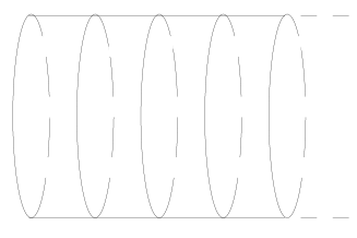
Figure 3: A lattice with one plaquette at each time.

To find the ground state, we can simply minimize (30) with a potential term $\int d\theta~{}\rho(\theta)~{}({1\over g^{4}a^{4}}(1-\cos\theta)-\mu)$ to find the ground state

$$\rho={N\over\pi}\sqrt{\mu-{1\over g^{4}a^{4}}(1-\cos\theta)}$$ (37)

with $\mu$ determined by $\int\rho=N$. Again we need to enforce the constraint $\rho(\theta)\geq 0$ on this solution by hand and there are two cases: for $g^{2}a^{2}>4/\sqrt{\pi}$ it is never saturated, while for $g^{2}a^{2}<4/\sqrt{\pi}$ there is a region around $\theta=\pi$ where it is. Thus this model has a large $N$ transition as well.

We could also have expanded $H/g^{2}$ in $\beta\equiv 1/g^{4}a^{4}$ to get the Hamiltonian strong coupling expansion, and resummed this expansion. In the string picture this is a source and one picture we can make is that we are summing world-sheets with $k$ ‘holes’ at order $1/(ga)^{4k}$, and integrating over the time in the target for each hole. Since the source is $O(N)$, terms involving $n$ cubic string interactions and $n+1$ sources are leading order.

To preserve the $D>2$ analogy, we can also postulate continuous world-sheet embedded in the ‘magnetic plaquette.’ It will have different weights from those in the original expansion: essentially, there are no branch points on the new world-sheet. One could enhance the analogy even more by taking the heat kernel action for the magnetic plaquettes, so the world-sheets would be generated with the same weights. This does not change the qualitative behavior.

Summing all disconnected diagrams will produce a coherent state for the ground state, of the form

$$|W\rangle=\exp\left({\sum_{n}{W_{n}\over n}\alpha_{-n}+{W_{-n}\over n}\bar{\alpha}_{-n}}\right)~{}|0\rangle$$ (38)

with $W_{n}$ determined from $\rho(\theta)$ in (37).

The exact result is analytic in $\beta$ near $0$, so summing the string diagrams will reproduce it. If we try to go past the transition by analytic continuation, we will produce a complex $\rho$, the continuation of (37) defined by simply ignoring the constraints.

Was this a failure of string theory or of the strong coupling expansion? Really, it is a failure of both. Built into the free string theory is the assumption that we can vary the occupation number of each winding number of string independently. What we see is that this can fail if the occupation number or amplitude is $O(N)$. This is the ‘non-perturbative structure’ we alluded to above. We can trace the failure back to the step where we decoupled the two fermi surfaces, a necessary step in deriving the bosonic theory.

Now the equivalence of (30) and (33) provides a more general rewriting the theory in terms of bosonic variables. We could call it ‘non-relativistic bosonization.’ This is particularly interesting in the present case, since the argument involving decoupling the fermi surfaces broke down at the turning point (where $\rho$ just reaches zero). This bosonization is exact in the classical limit, and (with careful treatment of the turning point) quantum corrections can be derived from (30) as well. This is the case relevant for the $c=1$ matrix model. [13]

We still cannot use this to fix up our original string theory, because we still need the constraint $\rho(\theta)\geq 0$ which cannot be expressed in string language. What it does suggest is that a broader idea of string theory might exist, and we will make some comments about this below.

In all the problems we discussed so far, and the one-matrix integrals, large $N$ transitions all appear exactly where we begin to saturate a constraint, $\rho(\theta)\geq 0$ or $\rho(p)\leq 1$. Let us see why these are two forms of the same underlying constraint.

Since the eigenvalues of $U$ are classical fermions in the large $N$ limit, we should be able to specify their positions and momenta simultaneously. Since they are indistinguishable, the state of the total system is given by a phase space density

$$\rho(\theta,p)=\sum_{i}\delta(\theta-\theta_{i})\delta(p-p_{i}).$$ (39)

Given this, $\rho(\theta)=\int dp~{}\rho(\theta,p)$ and $\rho(p)$ of (20) is ${1\over N}\int d\theta~{}\rho(\theta,p)$. The fermionic nature of the eigenvalues is exactly captured by

$$0\leq\rho(\theta,p)\leq{N\over 2\pi}.$$ (40)

Integrating $d\theta$, we see that the compactness of $\theta$ is responsible for the upper bound on $\rho(p)$.

The phase space description is more general and in many ways simpler than the collective field theory. [44] It can be derived from the quantum (non-relativistic) fermi theory using [14]

$$\rho(\theta,p)=\int d\alpha~{}e^{i\alpha p}~{}\psi^{+}(\theta-{\alpha/2N})\psi(\theta+{\alpha/2N}).$$ (41)

Any one body operator can be written directly as

$$\sum_{i}f(\theta_{i},p_{i})=\int d\theta dp~{}f(\theta_{i},p_{i})\rho(\theta,p).$$ (42)

(This can be used quantum mechanically and produces Weyl ordered operators.)

For the operators, the large $N$ limit is the standard classical limit. This is not necessarily true for the states – assembling $N$ classical fermions will produce states in which $\rho$ at each point is either $0$ or $\rho_{max}=N/2\pi$, but in general one can construct states in which $0<\rho<\rho_{max}$. An example is the state corresponding to a specific representation $R$, i.e. with wave function $\det z_{i}^{n_{j}}$. Such states are not coherent states of the form (38) and do not usually come up in practice.

The commutator of operators becomes Poisson bracket, a free particle bracket $\{f,g\}=2\pi(\partial_{p}f\partial_{\theta}g-\partial_{\theta}f\partial_{p}g)$. Time evolution is $\dot{\rho}=\{H,\rho\}$.

Collective field theory is derived by assuming a form

$$\rho(\theta,p)=\cases{{N\over 2\pi}&for $p_{-}(\theta)\leq p\leq p_{+}(\theta)$\cr 0&otherwise.\cr}$$ (43)

For example, $H={N\over 2\pi}\int dp~{}\rho(\theta,p){1\over 2}p^{2}$ reproduces (31). Again, the simple form of the state is an assumption, which is easily seen to be correct for problems such as (36). Several generalizations are possible. One can have a fermi surface of arbitrary shape, and a collective field theory using several functions $p_{i}(\theta)$ to describe it. There is also nothing special about the parameterization $p(\theta)$ and one could use $\theta(p)$ or $(\theta,p)$ depending on a parameter $s$ to describe the surface.

Free fermions are special to $D=1+1$ (and this system), but a language which in principle could generalize some of this to $D>1+1$ is known. [56] We can construct the phase space as the orbit of a reference state under the action of a ‘coherence group,’ obtained by exponentiating the Lie algebra of observables. Thus the entire kinematics of the limiting large $N$ theory is contained in the geometry of this group.

The discussion of [56] started from the basic observables of collective field theory, $\rho(\theta)$ derived from the invariant operators ${\rm tr\ }U^{n}$ and $\rho\partial\Pi(\theta)$ from ${1\over 2}{\rm tr\ }(EU^{n}+U^{n}E)$. These generated a semi-direct product of a Virasoro algebra with the modes of $\rho(\theta)$ and the corresponding group ${\rm Diff}(S^{1})$ semi-direct product the additive group of functions $\rho(\theta)$. The algebra generalizes directly to $D>1+1$ and in the next section we will be able to say something about the coherence group.

More recent work on these lines [14, 30, 7] uses all the one-body operators (42) to generate the group of symplectic diffeomorphisms on phase space, “${\rm SDiff}(2)$.” The idea that the canonical formalism is simpler if we consider all invariant operators made from $U$ and $E$, not just low powers of $E$, has not been studied in $D>2$, and might be valuable there as well.

So far, we have seen a relation in $D=1$ and $D=1+1$ between large $N$ transitions and constraints on the invariant observables. Similar constraints exist in higher dimensions. Essentially nothing is known about the phase space version, but the analog of $\rho(\theta)\geq 0$ is clear. Given any loop $L$ in space-time (or lattice), we can consider its holonomy $U(L)$ and associated spectral density $\rho_{L}(\theta)$: this should satisfy the same constraint. We will look at this in more detail in the next section.

It is natural to conjecture that large $N$ transitions are always associated with a change in the application of the constraints. Now, to have any hope of making a definite statement in higher dimensions, we need to find some qualitative conditions for the transition, that do not require exact results. Thus we might hypothesize that if for coupling $g_{1}$ the ground state saturates a constraint, and for $g_{2}$ it does not, there is necessarily a large $N$ transition in between.

This is an attractive hypothesis because it can be checked at strong and weak coupling where we have some control over the higher dimensional gauge theory. For strong bare coupling, $\rho_{L}(\theta)$ (for a loop on any scale) should saturate no constraints ($\rho>0~{}\forall\theta$), while at weak coupling and short distances the gauge field fluctuations are highly suppressed and we expect $\rho_{L}$ for small $L$ to have support sharply peaked about the origin (with width $\sim~{}g^{2}a/|L|$), no matter what regulator we use. This has been seen in the numerical studies [32, 6] and the finite radius of convergence of both diagram expansions makes it accessible analytically. The only doubt we might have regards the weak coupling phase, where to be precise we must be able to distinguish $\rho(\theta)=0$ from a very small but nonzero value, but let us imagine we can prove that (say) $\rho(\pi)=0$ for small loops.

One might think (and at Trieste I advocated the idea) that this would prove the existence of the large $N$ transition in higher dimensions, and the failure of the strong coupling expansion. We might expect $\rho_{L}$ for small loops to become complex, like (37), which looks very unphysical.

However, there are subtleties in this, as one realizes on considering the Wilson loop expectations in two dimensions on the plane. These are determined directly from the Boltzmann weight, $Z(U;A)=Z(U,1;A)$ as in (5):

$$W_{n}=\int dU~{}{\rm tr\ }U^{n}~{}\sum_{R}\chi_{R}(U)\dim Re^{-{A\over 2N}C_{2}(R)}$$

$$=\sum_{m=0}^{n}(-1)^{m}\dim Re^{-{A\over 2N}C_{2}(R)}$$

The sum is over the representations in the above figure. (This can be derived from fermionization: ${\rm tr\ }U^{n}|0\rangle=\sum_{m}b^{+}_{1/2-n+m}b_{-1/2-m}|0\rangle$.) Since the sum is finite, this will be analytic in $A$. (The string diagrams can have up to $n-1$ ‘ordinary’ branch points). If we compute $\rho(\theta;A)$ from these, we will find that it satisfies the conditions of the hypothesis: for $g^{2}A<4$, $\rho(\theta)$ has a gap around $\theta=\pi$, while for $g^{2}A>4$ it does not. [19] We might call this a ‘pseudo-transition’. It is visible in observables, but we need to look at Wilson loops winding arbitrarily many times to see it: at fixed $g^{2}A<4$, the $W_{n}\sim n^{-3/2}$ as $n\rightarrow\infty$, rather than falling exponentially.

We thus see that non-analyticity in the coupling for individual Wilson loop expectations and the existence of phase transitions cannot be concluded solely from the behavior of the spectral density, as pointed out long ago by B. Durhuus and P. Olesen. [19] Actually this does not directly contradict the hypothesis as stated, because the states in question are not ground states of the Hamiltonian. Nevertheless our belief in it may be somewhat shaken.

One can compute $\rho(\theta;A)$ more directly from the collective field theory. The problem was actually solved this way in [19], without ever mentioning collective field theory – they derived (45) directly from the Migdal-Makeenko equation.

Let us do ‘radial quantization’ on the plane, embedding the Wilson loops at fixed radius $r$, and and then go to the canonical formalism using $A=\pi r^{2}$ as time. Let us also finally redefine $\rho\rightarrow\rho/N$ from (30). $\rho(\theta;A)$ is thus the result of evolution for Euclidean time $A$ from the boundary condition $\rho(\theta;0)=\delta(\theta)$. It is simplest to think of going to Euclidean time in the action $S=\int dt\Pi\dot{\rho}-H$, by taking $t=iA$. To preserve the commutation relations in the Hamiltonian we should restore the first term by taking $\Pi\rightarrow-i\Pi$. It is then convenient to redefine

$$p_{\pm}=\partial_{\theta}\Pi\pm i\pi\rho$$ (44)

The equations of motion are the same (except for the $1/N$):

$$\partial_{A}p_{\pm}+p_{\pm}\partial_{\theta}p_{\pm}=0.$$ (45)

A nice simplification is now possible: since $\Pi$ and $\rho$ are real, the two equations are complex conjugate, and and if $p_{+}(\theta)$ is analytic, we have reduced the equation to a first-order ODE. Since $\rho(\theta)$ and $\Pi(\theta)$ are only prescribed on the real axis, there is generally no difficulty in finding such an analytic function.

We don’t know $\Pi$ at $A=0$ – it is not determined by the quantum initial condition $\psi(U)=\delta(U,1)$. In general, the classical limit of a Euclidean time quantum problem becomes a boundary value problem, where we specify (say) initial and final positions. The initial and final momenta are then determined only by solving the equations of motion. In general, more than one solution can exist with the same boundary conditions, and this is a possible source of phase transitions. All this applies to the large $N$ limit and in the present case we must specify the limiting behavior of $\rho$ as $A\rightarrow\infty$: it is the strong coupling vacuum $\rho(\theta)=1/2\pi$. (Similar considerations apply to the large $N$ limit of the Itzykson-Zuber integral, which as shown by A. Matytsin, can be expressed in terms of the same boundary value problem. [39])

Given only the boundary conditions, the explicit solution is not easy to find. However there is one more fact about the solution, which greatly simplifies the problem. After extending $p_{\pm}$ to be analytic functions in the complex $\theta$ plane, they fall off as $p_{\pm}\sim 1/\theta$ for large $\theta$, much like the resolvent ${\rm tr\ }(z-U)^{-1}$. Why this should be is not at all obvious from what we have said so far, but this assumption makes the problem easy, because then $\Pi$ at $A=0$ is determined by a dispersion relation, and we have an initial value problem. We can check the assumption at the end by verifying that it produces the correct $A\rightarrow\infty$ limit.

The final ingredient is to take periodicity in $\theta$ into account, which we can do by periodizing the initial condition. The analytic function satisfying ${\rm Im\hskip 1.00006pt}f=\pi\sum_{n}\delta(\theta-2\pi n)$ is then

$$f(\theta)={1\over 4\pi}\cot{\theta\over 2}.$$ (46)

The general solution of the Hopf equation can be derived by first representing the boundary $p_{+}(\theta)$ in phase space parametrically as $(p_{+}(\xi),\theta(\xi))$, implementing free motion $\theta(\xi;A)=\theta(\xi;0)+Ap_{+}(\xi)$, and solving for $\xi$. Although the pictures are simplest for real $p_{+}$, the solution is perfectly valid for complex $p_{+}$.

Thus, given an initial condition $p_{+}(\theta;A=0)=f(\theta)$, the solution is

$$p_{+}(\theta;A)=f(\xi(\theta;A))$$ (47)

where $\xi$ is the solution of the implicit equation

$$\xi(\theta;A)=\theta-Af(\xi(\theta;A))$$ (48)

We can then recover $\rho={1\over\pi}{\rm Im\hskip 1.00006pt}p_{+}=-{2\over A}{\rm Im\hskip 1.00006pt}\xi$.

This cannot be solved in closed form, but the comparison of $\rho(\theta)$ with (3) for $A\rightarrow\infty$, and the verification of the properties we described are not hard (and done explicitly in [19]). For example, to check that $\rho(\theta;A)\rightarrow 1/2\pi$ as $A\rightarrow\infty$, we can take the imaginary part of (48) and check that ${\rm Im\hskip 1.00006pt}\xi\rightarrow-A/4\pi$.

What is the essential difference between this problem and the sphere partition function? In this language, the sphere problem is formally very similar: it is a two-point boundary problem where both initial and final boundary conditions are $\rho(\theta)=N\delta(\theta)$.

Again, boundary value problems are not easy to solve, so we ask if another trick can convert this into an initial value problem. We can always extend $p_{\pm}$ into the complex $\theta$-plane as analytic functions, but now they cannot fall off as $p_{\pm}\sim 1/\theta$, simply because $\Pi$ is different in the two problems. I have not found such a trick and since I just want to illustrate the qualitative aspects of the problem, let us instead solve the problem for fermions on the real line. In other words we replace YM₂ by hermitian matrix quantum mechanics. In this case we already know the solution of the quantum problem with boundary conditions $\psi(M;t=0)=\delta(M)$: it is $|t\rangle\propto\exp-N{\rm tr\ }M^{2}/t$. Using this we can compute

$$\rho_{t}(\lambda)=\langle{T-t|{1\over N}\sum_{i}\delta(\lambda-\lambda_{i})|t}\rangle$$ (49)

and it is the saddle point spectral density for

$$\int\prod d\lambda_{i}~{}\Delta(\lambda)^{2}\exp-N({1\over t}+{1\over T-t})\sum_{i}\lambda_{i}^{2}.$$ (50)

This is

$$\rho_{t}(\lambda)={2\over\pi r^{2}}\sqrt{r^{2}-\lambda^{2}}$$ (51)

with $r^{2}(t)=4t(T-t)/T$. One can compute $\Pi_{t}$ similarly and check that the resulting

$$p_{+}(\lambda;t)={2\over r^{2}}\left((1-{2t\over T})\lambda-\sqrt{\lambda^{2}-r^{2}}\right)$$ (52)

is a solution of (45).

In fact, this is the weak coupling solution for the YM₂ sphere problem as well (found this way in [8]), with $T=A$. The periodicity $\theta\cong\theta+2\pi$ of eigenvalue space is completely invisible until we reach $r(A/2)=\pi$. This is the position space version of what we saw in section 2.

Once we reach $A=\pi$, the non-linearity of (45) means this is no longer a solution. In the phase space formalism this is due to the constraint $\rho\leq\rho_{max}$. One could do a calculation similar to that of the Wilson loop on $S^{2}$ [3, 12] to find the full strong coupling solution.

In this language, the difference between the two problems is subtle – the plane problem ‘knows about the compactness of eigenvalue space from the beginning,’ while the sphere problem ‘does not know until it hits the constraint.’ It all comes from the boundary conditions: whereas the sphere problem can be completely taken over to non-compact eigenvalue space, the final boundary condition for the plane $\rho(\theta)=1/2\pi$ only makes sense for compact eigenvalue space, and enforcing it affects the solution at all times.

The compactness enters in a slightly strange way in the initial value description: although the original problem was free fermions, which a priori would not know whether they were moving in compact or non-compact space, when we periodize the boundary condition (46), we change the motion around $\theta=0$, because (45) is non-linear.

The goal of this section was to study the large $N$ transition entirely in terms of invariant observables, since this language can generalize to $D>2$, and allows contact with a string reformulation. Clearly any conclusions we try to draw for $D>2$ will be speculative, but let us imagine we have a local continuum regulated gauge theory in $D>2$. We need a cutoff and thus the dependence of observables on length scale and coupling constant are not directly related. We will study it on ${R}^{D}$.

We can study the dependence on length scale by doing radial quantization of the theory, which turns scale dependence into ‘time’ dependence. Like the YM₂ expectations on the plane this should be a classical boundary value problem, and the large radius boundary condition provides a way for the system to ‘know’ about the non-trivial topology of configuration space and avoid a transition as a function of length scale.

On the other hand, the strong coupling expansion has no such mechanism – it only sees the limit $g\rightarrow\infty$ in which the constraints, the non-trivial structure of configuration space, are invisible. Thus summing it will produce results which have no reason to satisfy any constraints. The same conclusion would apply to any string reformulation in which the state with zero strings is the extreme strong coupling state $W_{0}(L)=N\delta_{L,I}$.  The true $W(L)$ is produced by summing string diagrams, and nowhere in this formalism are the constraints enforced.

YM₂ on the plane is a special case because the observables depend only on $g^{2}A$ and thus the first argument eliminates the transition in $g$.  At present, all we can infer from this is that the second argument does not prove there will be a transition.

What about a system in finite volume? Let us start by describing another way to understand the transition for $S^{2}$, developed by D. Gross and A. Matytsin [23]: it is driven by non-trivial classical solutions in the path integral. One can evaluate the path integral for $Z(S^{2})$ as a sum over classical solutions, using a non-abelian generalization of the Duistermaat-Heckman formula. [55] These are unstable solutions contained in $U(1)^{N}$ and constructed from the $U(1)$ instanton. (There is no $SU(N)$ instanton in $D=2$ as bundles over $S^{2}$ with gauge group $G$ are classified by $\pi_{1}(G)$.)

The $U(1)$ instanton is the configuration Dirac proposed as a monopole in $D=4$, restricted to constant $r$ and $t$. As usual for instantons in large $N$ gauge theory it has $O(N)$ action, from the explicit $N$ in $e^{-NS}$. However it can survive the large $N$ limit because of ‘entropy’ – each $U(1)$ factor has an independent instanton number – and in the strong coupling phase it does. This could be thought of as a covariant description of the ‘windings of eigenvalues around $S^{1}$’ which would appear if we made the classical fermion picture discussed here completely explicit.

Gross and Matytsin propose that the $D=4$ transition could also be driven by topologically non-trivial configurations, the standard instantons. In [23], they make a one-loop estimate of their effect as a function of the volume of the system (which controls the maximum of the running coupling) and find a result consistent with no phase transition. (See also [43]).

From the reasoning we gave earlier, we would conclude instead that we generally expect transitions as a function of volume in $D\geq 2$. At some critical volume, a mode will be strongly enough coupled to explore its full configuration space (e.g. $0\leq\theta\leq 2\pi$), new constraints will come into play, and new solutions of the collective field theory can exist. Now Gross and Matytsin are careful to state that they are arguing against a large $N$ instanton induced phase transition so there is no direct contradiction between these two statements: the instanton is certainly not the only field configuration which can explore the full configuration space.

In any case these questions must be considered unsettled, and the main point of my discussion is to outline considerations which we might be able to make precise given more control over $D>2$ collective field theory (or other loop equations). The main problem for now is to find a continuum regulated theory we can work with in $D>2$.

So far I have essentially been identifying ‘gauge string’ with ‘continuum strong coupling expansion.’ Now this is really an assumption and if it turns out that the strong coupling expansion is invalidated by a large $N$ or other phase transition, we would certainly want to change it.

What went into this assumption? The main element was the assumption that the state (or configuration – the discussion is really parallel in the canonical and covariant formulations) with no strings is the loop functional $W_{0}(L)=N\delta_{L,I}$.

As we saw, ‘strings’ are a reformulation of perturbation theory, not necessarily in the coupling, but in the sense that they describe $O(1)$ variations of an $O(N)$ initial configuration. Thus the choice of initial configuration to expand around is crucial. There is no way to describe constraints such as $\rho_{L}(\theta)\geq 0$ if we are restricted to statements expressable in perturbation theory around the extreme strong coupling state. This is a good motivation to change our zeroth order state.

One candidate which comes to mind is the extreme weak coupling state, $W_{1}(L)=N$ for all loops. Thinking about this leads us to ask the question, can standard weak coupling perturbation theory be reformulated as a theory of continuum world sheets, if we restrict ourselves to computing gauge-invariant observables? This is an interesting question which we will not discuss here. In any case this perturbation theory is seriously flawed by infrared divergences coming from the massless gluons. These do not cancel in all gauge-invariant quantities and no consensus has emerged as to whether it can be used even in principle for low energy physics.

Both starting points are handicapped by their serious qualitative differences with the true vacuum of the theory. Now in principle, we could imagine taking any loop functional $W_{g}(L)$ as our starting point for perturbation theory. It may not even be necessary for it to be the solution of some solvable limit of the theory. Let us write the true solution as $W(L)=W_{g}(L)+\delta W(L)$, and imagine deriving an expansion by plugging this into (29). In general we will get terms of order $(\delta W)^{1}$, $(\delta W)^{2}$ and if $W_{g}(L)$ does not solve the equation, $(\delta W)^{0}$. We will want to interpret the first and second terms as leading to a ‘string propagator’ and ‘string vertex’ – and the third term as a ‘string source,’ which might be modeled as holes in the world sheet, but much better as additional pieces of world-sheet with an action chosen to produce the correct dependence on $L$.

We could also change the association of small fluctuations of the loop functional $W(L)$ with ‘strings,’ as long as we preserve the locality of the resulting world-sheet theory.

To get new starting points, we need to have some non-perturbative way to construct loop functionals. Now the space of loop functionals is sometimes said to have little structure: one just specifies $W(L)$ for each $L$ satisfying $|W(L)|\leq N~{}~{}\forall L$. This is not true and in fact the space is not easy to describe in $D>1$. What is easier to describe are master fields.

4 Master Fields

Although we argued that taking advantage of factorization required us to restrict attention to $U(N)$ invariant quantities, in YM₂ it was very useful to talk about the holonomy for a given loop and its spectral density.

The higher-dimensional generalization of this is the ‘master field,’ a single gauge configuration $A_{\mu}(x)$ defined to reproduce all Wilson loop expectation values by evaluation: $W(L)={\rm tr\ }P\exp i\int_{L}A_{\mu}(x)dx^{\mu}$. Since the only assumption is factorization, the idea is also valid for large $N$ vector and matrix models, and the master field has been worked out for some vector models. [33]

Physicists have not had much success in writing explicit master fields for higher dimensional gauge theory or matrix models. It turns out, however, that recent mathematical work, specifically in the field of operator algebras, allows this to be done.

The most extensive work has been done by D. Voiculescu and collaborators. I will only give an introduction here, leaving out many interesting results, which are described very clearly in [52]. More recently, I. Singer has shown how to construct the master field for YM₂. [50]

The problem we discuss here is to compute leading order expectation values under integrals over several hermitian matrices $M_{i}=M_{i}^{+}$. Let the index range over the set $S$. Using factorization, the general case is

$$\langle{W}\rangle={1\over Z}\int~{}\prod_{\alpha\in S}d^{N^{2}}M_{\alpha}~{}e^{-NV}{}~{}~{}{1\over N}{\rm tr\ }W$$ (53)

where $W$ is an arbitrary ‘word’ or product of matrices

$$W =M_{\alpha_{1}}^{n_{1}}M_{\alpha_{2}}^{n_{2}}M_{\alpha_{3}}^{n_{3}}\ldots~{}$$

$$=\prod_{i=1}^{m}M_{\alpha_{i}}^{n_{i}}.$$

We will restrict ourselves to the case

$$V=\sum_{\alpha\in S}{\rm tr\ }V_{\alpha}(M_{\alpha}),$$ (55)

in other words no coupling between the matrices. Thus expectation values $\langle{{\rm tr\ }M_{\alpha}^{n}}\rangle$ are determined by the usual saddle point analysis and spectral densities $\rho_{\alpha}(\lambda_{\alpha})$, and this is hardly a ‘$c>1$’ matrix model. Nevertheless we have retained an aspect of the $c>1$ problem: the total number of words of a given length $l$, $|W_{l}|$, grows exponentially with $l$, and it is non-trivial to compute their expectations just given the $\rho_{\alpha}(\lambda_{\alpha})$.

Still, it is not very hard to do it – one can consider words with successively larger $m$ in (4), and write a chain of Schwinger-Dyson equations determining the case $m$ in terms of lower order expectations. Nevertheless this is rather unwieldy and one can ask for a simpler description of the result. This could be provided by a ‘master field’ – a set of single matrices “$\hat{M}_{\alpha}=\langle{M_{\alpha}}\rangle$” which we could regard as the saddle point for the integral (53). Now for each of the individual matrices, there is certainly a diagonal matrix with this property, but we cannot simply use this set: e.g. consider $V={\rm tr\ }A^{2}/2+{\rm tr\ }B^{2}/2$ for which

$$\langle{{\rm tr\ }A^{2}B^{2}}\rangle=N$$ (56)

while at leading $O(N)$

$$\langle{{\rm tr\ }ABAB}\rangle=0.$$ (57)

Now an integral like (53) is not literally dominated by a saddle point for the $M_{\alpha}$. If we write $M_{\alpha}=U_{\alpha}D_{\alpha}U_{\alpha}^{+}$, clearly fluctuations of the relative angular degrees of freedom $U_{\alpha}U_{\beta}^{+}$ are completely unsuppressed. On the other hand, the graphical argument for factorization can be made rigorous, and it is not clear why the heuristic arguments for the master field should fail.

The reconciliation of these two statements is that we can contruct a master field which behaves as if it were the saddle point. Let us do it for the case $V_{\alpha}(M_{\alpha})={1\over 2}{\rm tr\ }M_{\alpha}^{2}$.

We define the ‘free Fock space on $S$’ to be a Hilbert space with orthonormal basis vectors labelled by an ordered list of zero or more elements $\alpha_{j}\in S$. The elementary operators acting on this are $l_{\alpha}$ and $l_{\alpha}^{*}$ defined as follows:

$$l^{*}_{\alpha}|\alpha_{n},\alpha_{n-1},\ldots,\alpha_{1}\rangle =|\alpha,\alpha_{n},\alpha_{n-1},\ldots,\alpha_{1}\rangle\hfill$$ (58)

$$l_{\alpha}|\alpha_{n},\alpha_{n-1},\ldots,\alpha_{1}\rangle =\delta_{\alpha,\alpha_{n}}|\alpha_{n-1},\ldots,\alpha_{1}\rangle\hfill$$ (59)

$$l_{\alpha}|\rangle=0.$$ (60)

They are similar to bosonic creation and annihilation operators but with two differences. First, they are free – the product of two operators associated with $\alpha$ and $\beta\neq\alpha$ satisfies no relations. Second, the usual symmetry factor for bosonic harmonic oscillators is absent. Thus, we have not $[l,l^{*}]=1$ but instead

$$\sum_{\alpha}[l_{\alpha},l^{*}_{\alpha}]=|\rangle~{}{\langle}|.$$ (61)

On this Hilbert space, we define an operator $\hat{M}_{\alpha}$ associated with each $M_{\alpha}$, and a ‘trace’ $\hat{\rm tr\ }$. For the gaussian integral $V=M^{2}/2$,

$$\hat{M}_{\alpha}=l_{\alpha}+l_{\alpha}^{*}.$$ (62)

The ‘trace’ is not the standard one (which does not make sense here) but is defined by

$$\hat{\rm tr\ }A={\langle}|A|\rangle.$$ (63)

It is a trace in that it satisfies the axioms for a trace, for example $\hat{\rm tr\ }[A,B]=0$. (This is not yet obvious.)

One can see graphically that the construction works,

$$\hat{\rm tr\ }\hat{M}_{\alpha_{1}}\ldots\hat{M}_{\alpha_{m}}=\langle{{\rm tr\ }M_{\alpha_{1}}\ldots M_{\alpha_{m}}}\rangle,$$ (64)

by expanding the product of $(l_{\alpha_{i}}+l_{\alpha_{i}}^{*})$ in $2^{m}$ terms and associating a planar diagram with each non-zero term. Consider the example in figure 4. We start with $M_{\alpha_{m}=a}|\rangle$ which makes the state $|a\rangle$, and we interpret this as adding a line with the label $a$ to the diagram. With $M_{\alpha_{m-1}}$, there are in general two possibilities: we can always act with $l_{\alpha_{m-1}}^{*}$ to create a new line labeled $\alpha_{m-1}$, and if $\alpha_{m-1}=\alpha_{m}$ we can annihilate the existing line with $l_{\alpha_{m-1}}$ as well. The ‘free’ nature of the Fock space precisely reproduces the planarity constraint on the diagrams. After applying $M_{\alpha_{1}}$, we must be left with no lines to have a matrix element with ${\langle}|$. This proves (64), and since ${\rm tr\ }$ is a trace, so is $\hat{\rm tr\ }$.

Figure 4: Each non-zero term in the expansion of $\langle{\hat{\rm tr\ }\hat{M}_{b}\hat{M}_{a}^{2}\hat{M}_{b}\hat{M}_{a}^{2}}\rangle$ corresponds to a planar diagram.

The diagrammatic argument is a good demonstration but to gain insight from the use of master fields we need new concepts. The central concept in Voiculescu’s work is that of ‘free probability distribution.’ This is analogous to the idea of independence in probability theory: a set $\{x_{\alpha}\}$ of commuting random variables is independent if the joint expectations $\phi(f_{1}(x_{1})\ldots f_{n}(x_{n}))=\phi_{1}(f_{1}(x_{1}))\ldots\phi_{n}(f_{n}(x_{n}))$.

Let us regard our matrix model expectation values $\langle{{\rm tr\ }W}\rangle$ as giving the joint expectations $\phi(W)$ for words constructed from a set $\{M_{\alpha}\}$ of non-commuting random variables. We normalize $\phi(1)=1$. The distribution is free if

$$\phi(~{}f_{i}(M_{\alpha_{i}})~{})=0\qquad i=1,2,\ldots m~{}~{}{\rm and}$$ (65)

$$\alpha_{i}\neq\alpha_{i+1}~{}~{}\forall i\qquad$$

imply

$$\phi(~{}f_{1}(M_{\alpha_{1}})~{}\ldots~{}f_{m}(M_{\alpha_{m}})~{})=0.$$ (66)

Just as for independence, given the individual distributions this assumption completely determines the joint distribution. The general expectation $\phi(~{}f_{1}(M_{\alpha_{1}})~{}\ldots~{}f_{m}(M_{\alpha_{m}})~{})$ can be computed by induction. Let $g_{i}(M_{\alpha_{i}})=f_{i}(M_{\alpha_{i}})-\phi({f_{i}(M_{\alpha_{i}})})$ so that $\phi({g_{i}(M_{\alpha_{i}})})=0$; then by substituting $f_{i}=\phi({f_{i}})+g_{i}$ for all $i$, distributing and using (66) on $\phi(g_{1}\ldots g_{m})$, we can reduce it to a sum of terms with fewer components.

Expectations of the large $N$ limit of decoupled matrix integrals with (55) are free. This can be proven diagrammatically, by induction on the number of components: given (65), to get a non-zero expectation we must take diagrams with a line connecting two components, and this splits the diagram into a product of expectations with fewer components. It has been proven in [52] for a broader class of decoupled measures.

Freeness can be implemented directly in the master field: given the individual master fields for the individual matrix integrals, which we already know, the joint master field is their ‘free product.’ This can be defined algebraically using the ideas we already described: the essential point is that $\hat{M}_{i}$ and $\hat{M}_{j}$ satisfy no relations.

To fit this into a larger context, we will change our language slightly: we should think of the master field as a representation of the abstract algebra generated by the $M_{\alpha}$’s, and $\phi({A})$ as a linear functional on this algebra. Many of the usual ideas of representation theory, such as unitary equivalence, are directly relevant here. As we will see later, this language is also well suited to the gauge theory case.

The relevant algebra for a hermitian matrix integral is the algebra of functions of a single real variable $\lambda$. For mathematical purposes of course we would want to be more precise. I will not try to be so precise, but at least for our cultural benefit let us look at the algebras which come up. For a one-matrix distribution, $M$ is represented by the operator of multiplication by $\lambda$ (its spectral parameter), and $\phi({f})=\int d\lambda~{}\rho(\lambda)f(\lambda)$. This only sees a subset of ${R}$, the spectrum of $M$ (support of $\rho$), so we could equally well use the algebra of functions on ${\rm Spec}M$. One natural object to consider is the algebra of bounded continuous functions on ${\rm Spec}M$. This can be made into a $C^{\ast}$-algebra by using the sup norm. (For the defining axioms of a $C^{\ast}$-algebra, see for example [42].) $C^{\ast}$-algebras are the most tractable general class of algebras, and this is quite useful. It is a theorem that every commutative $C^{\ast}$-algebra is an algebra of bounded continuous functions on some space $M$, and one can recover the topology of $M$ from the algebra $C^{0}(M)$. In matrix models, it can be relevant to the physics to know the number of components of ${\rm Spec}M$ (e.g. one-cut v.s. two-cut matrix models) and their topology, and perhaps analogous concepts of the ‘non-commutative topology’ of the algebras arising in multi-matrix models or matrix field theories will eventually be relevant.

Since we have a measure, another natural algebra to consider is that of the $L^{\infty}$ functions, bounded in the norm $||f||_{\infty}=\lim_{p\rightarrow\infty}\left(\int d\lambda~{}\rho(\lambda)|f(\lambda)|^{p}~{}\right)^{1/p}$. This is both a $C^{\ast}$-algebra and a von Neumann algebra. These functions need not be continuous and this algebra retains very little information about the topology of the underlying space.

Usually for us ${\rm Spec}M$ is a bounded set $I$, so we can restrict attention to $C^{0}(I)$ or $L^{\infty}(I)$. This last is isomorphic as an abstract algebra to $L^{\infty}(S^{1})$, and by Fourier transform to $L({Z})$, the group algebra of ${Z}$. Now we can appeal to a result of [52] which I hope will sound intuitive: the free product of group algebras is the algebra of the free product of groups. The free product ${Z}*{Z}\ldots$ ($n$ times) is the free group on $n$ generators, $F_{n}$. Thus the von Neumann algebra which arises in an $n$-matrix problem is $L(F_{n})$.

It is conceivable that other algebras could come up. For example, in the large $N$ limit of Chern-Simons theory, [17] one expects Wilson loop expectations on $\Sigma\times I$ (for $\Sigma$ a Riemann surface) to give a functional on $L(\pi_{1}(\Sigma))$. In general, we know that we will get a ‘type ${\rm II}_{1}$ algebra in the Murray-von Neumann classification.’ This just means that there is a trace taking values (on positive operators of norm one) in $[0,1]$. One also has a notion of ‘factor,’ an algebra with trivial center, which implies that this trace is unique. This may sound attractive for our purposes but at this point one starts getting into subtleties, in particular involving the choice of norm used in defining the algebra. There are many definitions of $C(F_{n})$ (for $n\geq 2$): some are factors (e.g. the ‘reduced’ algebra), and others are not (e.g. the ‘full’ or ‘universal’ algebra). The only point I will take from this is the obvious one that one needs to be careful to check that one’s definitions are appropriate.

Returning to a single matrix, another description of the same representation which makes contact with our free Fock space is to write a series

$$\hat{M}_{\alpha}=l_{\alpha}+\sum_{n\geq 0}c_{n}l^{*n}_{\alpha}$$ (67)

satisfying $\hat{\rm tr\ }\hat{M}_{\alpha}^{k}=\int d\lambda\rho(\lambda)\lambda^{k}.$ Clearly such a thing exists in general, because the $k$’th moment is determined by $c_{n}$ with $n\leq k-1$. The free product of these representations can then be taken by letting these operators act on the free Fock space.

One can show [52] that the $c_{n}$’s are determined as follows: given the resolvent $F(z)=\phi({1\over z-M})=\int{d\lambda\rho(\lambda)\over z-\lambda}$, compute the inverse of $F(z)$ under composition, $K(F(z))=z$. Then

$$K(x)\equiv{1\over x}+{\cal R}(x)={1\over x}+\sum_{n\geq 0}c_{n}x^{n}$$ (68)

For example, the semicircle distribution has $F(z)={2\over r^{2}}(z-\sqrt{z^{2}-r^{2}})$ giving ${\cal R}(x)={r^{2}\over 4}x$.

Thus, the operators (67) acting on free Fock space are the master field for any decoupled set of matrix integrals. What can we do with this? A problem treated in [52] is the following: find the moments $\phi({(\sum_{\alpha}M_{\alpha})^{n}})$, or equivalently the spectral density for $\sum_{\alpha}M_{\alpha}$. In ordinary probability theory, the resulting distribution would be the convolution of the independent distributions; thus the new concept can be called ‘free convolution’ (or ‘additive free convolution’).

It is clear that if we add two free variables, the result will be free with respect to the rest, and the addition is commutative and associative. Thus we need only consider binary free convolution. The result which determines it is the following: the operators

$$\hat{M}_{1}+\hat{M}_{2}=l_{1}+l_{2}+\sum c_{1,n}l_{1}^{*n}+c_{2,n}l_{2}^{*n}$$ (69)

have the same distribution as

$$\hat{M}_{1+2}=l+\sum(c_{1,n}+c_{2,n})l^{*n}.$$ (70)

This is not hard to see, by explicitly writing out a term like $\langle{|(\hat{M}_{1}+\hat{M}_{2})^{k}|}\rangle=\langle{|(l_{1}+l_{2}+\ldots)^{k}|}\rangle$ and noting that any place an annihilation operator appears, exactly one of $l_{1}$ or $l_{2}$ will contribute. Thus

$${\cal R}_{1+2}(x)={\cal R}_{1}(x)+{\cal R}_{2}(x).$$ (71)

For example, the free convolution of semicircles with radius $r_{i}$ is a semicircle of radius $r^{2}=\sum r_{i}^{2}$.

In [52] an analogy is developed between the Gaussian in ordinary probability theory and the semicircle law in free probability theory. For example, there is an analog of the central limit theorem: given a free family of distributions $\phi_{i}$, with $\phi({M_{i}})=0$, all higher moments bounded, and $\lim_{n\rightarrow\infty}{1\over n}\sum_{i=1}^{n}\phi(M_{i}^{2})=r^{2}/4>0$, the sum ${1\over\sqrt{n}}\sum_{i}M_{i}$ converges on a semicircle with radius $r$. Such results might help explain the ubiquity of the GOE and GUE in statistics of energy levels of random Hamiltonians.

So far we have been considering free products of one matrix distributions but the concept is more general: for example, we could take the free product of $\phi$ with arbitrary dependence on $M_{1}$ and $M_{2}$, with $\psi$ depending on $M_{3}$. In full generality we could talk about a free family of subalgebras $A_{i}$ of the full algebra of ordered products: in (66), the successive components would be required to belong to distinct subalgebras.

Let us use these techniques to give another derivation of (45), here for quantum mechanics of a hermitian (rather than unitary) matrix. (This is very similar to [53]). We start with a discretized path integral:

$$Z=\int\prod_{i=1}^{L}dM(i)~{}e^{-N\sum_{i}{\rm tr\ }(M(i+1)-M(i))^{2}/\epsilon}$$ (72)

with $t=\epsilon L$. Given an initial condition $M(0)$, this determines

$$M(t)=M(0)+\epsilon\sum_{i=1}^{L}\eta(i)$$ (73)

where the $\eta(i)=M(i)-M(i-1)$ are free random variables with semicircular distribution. Let $\rho_{t}(\lambda)$ be the resulting spectral density at time $t$, and define $F_{t}$ and $K_{t}$ from it as above. We can compute $K_{t}$ using (71) in terms of the initial condition $K_{0}(u)$:

$$K_{t}(u)=K_{0}(u)+\epsilon Lu$$ (74)

Changing variables from $u$ to $\xi=K_{0}(u)$,

$$K_{t}(F_{0}(\xi))=\xi+tF_{0}(\xi)$$ (75)

Let us define $z(\xi,t)=K_{t}(F_{0}(\xi))$. Applying $F_{t}(z)$ to both sides of this definition, we have

$$F_{t}(z)=F_{0}(\xi)$$ (76)

and we have reproduced (47) with $F_{t}(z)=p_{+}(z,t)$. Finally, substituting into (75) produces (48), the general solution of (45).

Notice that this derivation only required an initial condition and produced the Hopf equation directly for the resolvent ${\rm tr\ }(z-M)^{-1}$. Perhaps we have found a better explanation for the condition $p_{\pm}\sim 1/\theta$ we found in YM₂ on the plane? That result was almost the same but with periodic $\theta$ – can we derive it in this spirit?

One can imagine calculating the master field for the holonomy in figure 5 by summing graphs in axial gauge. This would produce an evolution similar to (73), but operating by multiplication:

$$U(t+\epsilon)=e^{iA(t,0)}U(t)e^{-iA(t,L)}$$ (77)

with the $\{A(t,x)\}$ at different times free with respect to each other. This should be calculable using ‘multiplicative free convolution,’ another concept developed in [52].

Figure 5: Time evolution in YM₂.

A direct field theory application of this is to Gaussian matrix models (free in the physics sense). The $D$-dimensional matrix field theory with (Euclidean) action

$$S={N\over 2}{\rm tr\ }\int d^{D}x(\partial_{i}M)^{2}+{m^{2}}M^{2}$$ (78)

is a free product of semicircular distributions for each mode $A(k)+iB(k)=\int d^{D}xe^{ikx}M(x)$.

It is not clear whether freeness plays any direct role in non-trivial higher dimensional field theories, but it may be possible to use free distributions indirectly to construct their master fields. A construction of this type was given by J. Greensite and M. Halpern: let us discuss it briefly. [22]

A general field theory can be formulated using stochastic quantization: [11] the $\tau\rightarrow\infty$ limit of the solution of the Langevin equation

$${\partial\over\partial\tau}\hat{\phi}(x)=-{\partial S\over\partial\hat{\phi}(x,\tau)}+\eta(x,\tau),$$ (79)

where $\eta(x,\tau)$ is a Gaussian random variable with correlation $\langle{\eta(x_{1},\tau_{1})\eta(x_{2},\tau_{2})}\rangle=2\delta(x_{1}-x_{2})\delta(\tau_{1}-\tau_{2})$, reproduces quantum expectations, $\langle{\hat{\phi}(x)\ldots}\rangle_{\eta}=\langle{\phi(x)\ldots}\rangle_{\phi}$.

For $\hat{\phi}$ a hermitian matrix, the $\eta(x,\tau)$ become free random variables in the large $N$ limit. (Greensite and Halpern represented them using explicit Gaussian matrix integrals.) Thus we can regard (79) as a ‘free non-linear PDE’ for which the $\tau\rightarrow\infty$ limit of a solution is a master field. This is an equation with some similarity to (73), and perhaps one could find free analogs of the existing techniques to solve non-linear PDE’s (a particularly interesting idea for integrable theories).

Let us at least solve the linear case: for (78), we can Fourier decompose $\hat{\phi}=M$, and proceeding as we did with (73) for each mode, find that

$${\partial\over\partial\tau}K_{\tau}(k;u)=-(k^{2}+m^{2})K_{\tau}(k;u)+u.$$ (80)

The solution is $K_{\tau}(k;u)=u/(k^{2}+m^{2})+Cue^{-(k^{2}+m^{2})\tau}$ which for $\tau\rightarrow\infty$ corresponds to the semicircle we mentioned earlier.

Another possible use of free expectations would be as ansatzes or as starting points for perturbation theory. An example of something we can get this way is a gauge theory loop functional which interpolates smoothly between ‘weak coupling’ behavior of the spectral density at high momenta and ‘strong coupling’ behavior at low momenta. It is just defined by the integral $\int dA\exp-\int d^{D}k{\rm tr\ }f(k,A_{\mu}(k)A^{\mu}(-k))$ (with $A_{\mu}(-k)=A_{\mu}(k)^{*}$). $f(k,z)$ can be chosen arbitrarily and to get the required property we would take it to interpolate between $f(k,z)\sim k^{2}z$ at large $k$, and (say) $f(k,z)\sim k^{2}\cos\sqrt{z}$ at small $k$.

The ansatz is rather ugly, especially with its ad hoc gauge fixing. Nevertheless it does define a master field and all Wilson loop expectations can be computed from it. A possible application for it would be as a ‘building block’ for more general loop functionals, to which we turn.

There is a more general construction, by which if one is given all expectation values of invariant operators, one can construct a master field which reproduces them. This has been done by I. Singer for a continuum gauge theory, specifically YM₂. [50] Let us discuss an analogous construction in lattice gauge theory. (One can also adapt it for matrix models.) In this case, the gauge holonomy is a representation of the groupoid of paths on the lattice. For the present discussion (this can be generalized) we fix an ‘axial’ gauge by choosing a spanning tree $T$ of the lattice, and setting these links to $\bf 1$. The holonomy is then determined by its values on the graph formed by contracting $T$ to a point $t$; this graph is a ‘bouquet’ of circles attached at $t$ and paths starting and ending at $t$ generate a free group algebra. Thus $W(L)$ is a functional on the free group, and we define its values on a general element of the algebra by linearity.

The construction of the master field is the GNS (Gel’fand-Naimark-Segal) construction [42] and once one has phrased the expectation values as a linear functional on the group algebra, it applies straightforwardly. The regular representation $\pi$ of the algebra $A$ acts on a vector space ${\cal H}\cong A$ by

$$\pi(a)|b\rangle=|ab\rangle.$$ (81)

Essentially, we want to make this a Hilbert space with the inner product

$$\langle{a|b}\rangle=W(b^{*}a)$$ (82)

and define

$${\rm tr\ }\pi(a)=\langle{I|\pi(a)|I}\rangle.$$ (83)

(We are labelling vectors by the associated element of $A$, and $I$ is the identity element in the group.)

The master field will be the representation $\pi(L)$. Its defining property is that ${\rm tr\ }\pi(L)=W(L)$; this is almost a tautology and in this sense we only ‘repackaged’ the information of the loop functional. But there is more to check, because we need the inner product to be positive definite, $\pi$ to be a unitary representation, and ${\rm tr\ }$ to have cyclic symmetry.

The first condition clearly will not hold for just any $W(L)$: it must satisfy a positivity condition. Now positive definiteness of the inner product would follow from $W(a^{*}a)>0~{}\forall a$, but it is clear that semi-positive definiteness

$$W(a^{*}a)\geq 0\qquad\forall a$$ (84)

is all we can expect in general. Let’s reconsider the $D=1$ case: loops are classified by winding number and their group is ${Z}$; the positivity condition is

$$\sum_{n,m}W_{n-m}f_{n}f^{*}_{m}\geq 0\qquad\forall f_{n}.$$ (85)

We can turn the convolutions into multiplication by considering $\rho(\theta)=\sum_{n}W_{n}e^{in\theta}$ and $f(\theta)$, in terms of which (85) becomes

$$\int d\theta\rho(\theta)|f(\theta)|^{2}\geq 0$$ (86)

which is our old positivity condition.

One can define a positive element $p$ of an operator algebra as one whose eigenvalues are positive in any representation, or more abstractly by requiring its spectrum (this is defined without appeal to any representation as $\{\lambda|(p-\lambda)^{-1}\notin A\}$) to be contained in the positive real axis. An element $p=a^{*}a$ will be positive, and it is a theorem for $C^{\ast}$ algebras that any positive element can be written in this way. One refers to $W$ as a positive linear functional if it is positive on the positive elements.

We now deal with the semi-definite case by finding the ideal of elements $\{z|W(z^{*}z)=0\}$ and quotienting the space ${\cal H}$ by this ideal. In the one matrix case, the quotient is the algebra of functions on ${\rm Supp}~{}\rho$. The inner product (82) is positive definite on the quotient and there is a unique completion of the quotient which is a Hilbert space. The result is a unitary representation. Unitarity $u^{\ast}=u^{-1}$ follows because it was true in the abstract algebra.

Finally, ${\rm tr\ }[a,b]=\langle{1|[a,b]|1}\rangle=W([a,b])=0$. Thus the representation $\pi(L)$ is a master field.

Not every loop functional has a master field, because of the positivity requirement. A (unitary) quantum field theory vacuum, however, will. First, the contribution from any point in field space is positive: by definition, a positive $L$ must have positive eigenvalues in any representation, and thus ${\rm tr\ }U(L)$ (for positive $L$) will be positive for any $U$. Then, expectation values under a functional integral with positive measure will be positive, so these will be associated with master fields.

If we need to deal with a non-positive loop functional (say a perturbation of the ground state), we can construct a ‘virtual master field’ which is a pair of fields $U_{1},U_{2}$ such that $W(L)={\rm tr\ }U_{1}(L)-{\rm tr\ }U_{2}(L)$. It can be proven that this exists for any real $W(L)$, and that a similar construction with four $U_{i}$ can reproduce any complex functional.

If we regard the large $N$ theory as being defined by a loop equation, e.g. the Migdal-Makeenko equation or equations derived from a collective Hamiltonian, we should regard the positivity constraint as an additional element of the definition. It is non-trivial, non-perturbative structure of the configuration space. To some extent it is independent of the loop equation, and when we solve the equation we may need to enforce the constraints by hand, as we discussed in the previous section.

These inequality constraints are rather simpler than the Mandelstam constraints on loop functionals constructed from gauge fields at finite $N$ – for example, there are cases (loop functionals near the strong coupling limit) in which they are irrelevant. It was known in earlier work that such constraints exist and important, [32, 6] and the description given there had some similarities: when the change to loop variables is non-singular, the metric on configuration space ($h_{ij}$ of section 3) in these variables,

$$\Omega(L,L^{\prime})=\sum_{L^{\prime\prime}}{\rm tr\ }[E_{L}^{\prime\prime},W(L)][E_{L}^{\prime\prime},W(L^{\prime})]$$ (87)

will be positive definite. The constraint (84) is a bit stronger than (87) (in $D>2$) because it does not have the sum over $L^{\prime\prime}$. It is simpler to think about, most importantly because it is obviously linear. It is also clear that positivity requires positivity for any subgroup of the group of loops.

Let us illustrate it on a ‘figure eight,’ a bouquet of two loops $l_{1}$ and $l_{2}$ with holonomies $U_{1}$ and $U_{2}$. Besides a list of the $W(L)$, an equivalent form of the data is to specify

$$W(l_{1}^{p_{1}}l_{2}^{q_{1}}\ldots l_{1}^{p_{m}}l_{2}^{q_{m}})=\qquad$$ (88)

$$\qquad\int d\theta_{i}d\phi_{i}~{}\rho_{m}(\theta_{i},\phi_{i})e^{i\sum p_{i}\theta_{i}+q_{i}\phi_{i}}.$$

The simplest new case of (84) is to let $a=\sum_{m,n}c_{m,n}l_{1}^{m}l_{2}^{n}$: these can be combined to show that $\rho_{1}(\theta_{1},\phi_{1})\geq 0$. We could also derive this from a spectral decomposition $U_{i}=\int d\theta~{}\rho_{i}(\theta)P_{i}(\theta)$ over projections $P_{i}(\theta)^{2}=P_{i}(\theta)$, using ${\rm tr\ }P~{}P^{\prime}\geq 0$. However the pattern does not generalize: the next constraints, derived from $a=\sum_{l,m,n}c_{l,m,n}l_{1}^{l}l_{2}^{m}l_{1}^{n}$, are too weak to force $\rho_{2}$ to be positive. It is not hard to construct examples in which it is not, using projections such that ${\rm tr\ }P~{}P^{\prime}~{}P^{\prime\prime}<0$.

Although this does illustrate that (84) contains new information, this particular explicit form does not look too useful. Another illustration of the difficulties of working explicitly with (84) is the following: there are functionals on a bouquet of $k$ loops which satisfy the constraints defined in terms of $l<k$ loops, but violate constraints involving $k$ loops.

A loop functional constructed from a master field automatically satisfies the constraints, and (as was noted in previous work) the simplest description of the configuration space is the space of all master fields up to gauge equivalence, or (what is the same thing) the space of unitary representations of the free group algebra up to unitary equivalence.

An important issue in working with $D>2$ large $N$ theories is the choice of representation of loop functionals – for both analytical and numerical purposes we need truncations which allow approximating a loop functional with a finite amount of information. If constraints are saturated, it is clear (already in $D=2$) that specifying the functional on all loops up to a given length is inappropriate. One alternate proposal in earlier work was to work with a finite-dimensional approximation to the master field and derive the loop functional from it. Another style of representation is to build loop functionals up from simple functionals. Since the space of loop functionals really is a linear space, it makes sense to propose a basis for loop functionals. One might try to find a basis of ‘extreme points’ in the space of functionals, from which any positive functional could be made by superposition with positive coefficients.

Simple operations which preserve positivity are addition of loop functionals, and loopwise multiplication $(W_{1}\times W_{2})(L)=W_{1}(L)W_{2}(L)$. Formally, the corresponding master fields are just the direct sum and direct product of those for $W_{1}$ and $W_{2}$. Although we have not precisely defined continuum master fields, it is interesting to note that in the continuum, if $A_{1}$ and $A_{2}$ are solutions of the classical Yang-Mills equations, both direct sum and direct product will produce a new solution. This explains the observation of A. Migdal that the left hand side of the Migdal-Makeenko equation (29) is a first order linear operator on loop functionals. [40]

There is a similar idea of ‘phase space master field’ which reproduces expectation values of invariant operators made from $\vec{A}(\vec{x})$ and $\vec{E}(\vec{x})$, or for matrix models $M(\vec{x})$ and its conjugate $\Pi(\vec{x})$, as used in [1, 6]. Issues of operator ordering make this rather more subtle to study, but we intend to discuss it in future work.

Let us discuss a simpler question raised in the last section: what is the higher dimensional analog of the Virasoro algebra of matrix quantum mechanics, and the corresponding group? The generators are known:

$$\Pi(f,x)={\rm tr\ }f(M)\Pi(x)$$ (89)

where $f(M)$ can be an arbitrary word in the $M$’s (but not the $\Pi$’s). Their algebra is easy to compute as is their action on the invariant observables $\phi(W)={\rm tr\ }M(x_{1})\ldots M(x_{m})$:

$$[\Pi(f,x),\phi(W)]=\sum_{i}\delta_{x,x_{i}}$$ (90)

$${\rm tr\ }M(x_{1})\ldots M(x_{i-1}) ~{}f~{}M(x_{i+1})\ldots M(x_{m})$$

Can we generalize to $D>1$ the identification of this as the infinitesimal diffeomorphism $\delta\lambda=f(\lambda)$ ? In terms of the master field, the generalization is

$$\delta M(x)=f(M)$$ (91)

and we should think of this transformation as an ‘infinitesimal free diffeomorphism.’

It is an infinitesimal automorphism of the free group algebra $C(F_{n})$: it is linear and a derivation, and $\delta M^{+}=(\delta M)^{+}$ implies it is an automorphism of the $C^{\ast}$ algebra. Thus the corresponding group is the automorphism group of the free group algebra (or possibly the connected component of the identity), and the coherence group is a semidirect product of this with the additive group in the algebra.

Returning to configuration space, a simple but important master field for gauge theory reproduces the extreme strong coupling limit, the loop functional $W(L)=\delta_{L,I}$. It is just the regular representation with the conventional inner product $\langle{L_{i}|L_{j}}\rangle=\delta_{i,j}$ in a basis of loops. It saturates no constraints: by adding sources to the functional integral we can make small variations of the $W(L)$ for every $L$ independently.

The first observation to make is that this master field is a representation on a very large Hilbert space, not just infinite but ‘more infinite’ than even a quantum field theory Hilbert space. What I mean by this is that in terms of the natural grading, namely by word length, the degeneracy of states grows exponentially as $(2D-1)^{l}$. (For quantum field theory in dimension $D$ and with finitely many fields, the degeneracy of states grows as $\exp E^{1-1/D}$.) It is the same linear space in which variations of the loop functional live and we can (by analogy with string field theory) also think of it as the ‘first quantized string Hilbert space.’ From this point of view, exponential growth is the expected result for a string theory. However there is an important difference with the better understood case of fundamental string theory: although there we also have exponential density of states in terms of space-time energy, the world-sheet grading is not by space-time energy but by world-sheet ‘energy’ $n=\alpha^{\prime}m^{2}$, and thus world-sheet densities of states have the familiar $\exp\sqrt{n}$ behavior.

Now the grading which is relevant in string perturbation theory is that given by the world-sheet Hamiltonian, and we don’t know this for gauge strings. (We do know it in light-front quantization, at least if we call the states ${\rm tr\ }O_{i}|0\rangle$ ‘strings,’ and there the world-sheet Hamiltonian determines $m^{2}$.) Thus it is not yet clear if this has relevance for physics. It turns out to be very relevant for mathematics, however. Consider the following question: since we found that the extreme strong coupling master field is simply the regular representation of the group algebra, why not follow the normal procedures of group representation theory and decompose this representation, which for compact Lie groups contains copies of every irreducible representation?

In fact this representation is irreducible. Many standard statements of representation theory break down for such large groups. Technically, free groups are not amenable, a statement whose definition I leave to [21, 9]. Apparently, little is known about the space of all of its representations.

5 Parting thoughts

A lot of work on large $N$ in $D>2$ has concentrated on trying to solve models or at least develop reliable numerical procedures for treating loop equations. This is an attractive goal, not just for gauge theory but in my opinion even more so for matrix models and string theory, because there the main difficulty we face – the large number of degrees of freedom – is not an artifact of our approximation but an essential feature of the problem we are studying.

We appear to be far from this goal, and I believe that a certain amount of mathematical ground work will be required first, because the objects we are working with are so unfamiliar. Thus I want to conclude by proposing a simpler application of the loop space formalisms than ‘solving’ a large $N$ field theory: to be the starting point for new perturbative expansions, and to better understand the expansions we have. These are problems which require some ability to work with the theory non-perturbatively, may well lead to practical calculational techniques, and could give us a better starting point for more ambitious work.

The prototype for ‘gauge string theory’ is the strong coupling expansion. The recent work suggests that this old formalism can be greatly improved, most notably by formulating it in the continuum. We need to continue it to weak coupling, but if it is qualitatively correct, as perhaps it could be, there would be no fundamental barrier to doing this. However, to use it one must justify not only the expansion around infinite coupling but also the assumption that the difference between the starting loop functional $W_{0}(L)=\delta_{L,I}$ and the result $W(L)$ is ‘small’ – not necessarily in magnitude, but in the sense that no new structure of the configuration space or action is required to get the correct result. As we saw, these issues are much simpler for large $N$ gauge theories than for finite $N$ gauge theories, but still non-trivial, and in the end this assumption was found to be highly suspect – there is new structure in the form of linear constraints on physically realizable loop functionals, which is not visible in strong coupling, and probably leads to a large $N$ transition analogous to those in the solvable models.

We should think of ‘string’ as a perturbative construct, describing a small fluctuation of the fields, very analogous to particles in quantum field theory. Thus we should not try to fix the original string construction but instead define a new construction in which we expand around a different zeroth order loop functional, e.g. one which saturated the right constraints. Changing this could produce a very different string theory. (See [17] for an extreme case of this.)

Another, more conventional motivation for expanding around non-trivial configurations, is to get the physics right in the zeroth order. A different direction would be to try to fix the obvious flaws of the weak coupling expansion for gauge theory, such as the masslessness of the gluons, by starting it around a non-trivial background.

To do any of this we need to better understand loop functionals and master fields, and I hope I have convinced the reader that there are interesting things which can be done in these directions. I believe this would also be invaluable for matrix models of fundamental strings – after all, the real point to finding a $c>1$ matrix model is to make non-perturbative statements using it, and surely the first step towards this is to have some non-perturbative picture of its configuration space. But these are problems for the future.

It is a pleasure to acknowledge valuable discussions with M. Halpern, V. Kazakov, I. Kostov, A. Migdal, G. Moore, H. Neuberger, A. Polyakov, M. Staudacher, W. Taylor, and K. Woo, and I especially thank I. Singer and D. Voiculescu for discussing their work with me. I also want to express my gratitude to the organizers of the Spring School, and to the students for their interest and for their patience.

References

- [1] K. Bardakci, Nucl.Phys. B219 (1983) 302 and references there.
- [2] Z. Bern, M.B. Halpern, L. Sadun and C. Taubes, Phys.Lett. B165 (1985) 151; M.B. Halpern and Yu.M. Makeenko, Phys.Lett. B218 (1988) 230;
- [3] D. Boulatov, Mod.Phys.Lett.A9 (1994) 365.
- [4] E. Brezin and D. J. Gross, Phys.Lett. 97B (1980) 120.
- [5] E. Brezin, C. Itzykson, G. Parisi and J.-B. Zuber, Comm.Math.Phys 59 (1978) 35.
- [6] F. Brown and L. Yaffe, Nucl. Phys. B271 (1986) 267; T. A. Dickens, U. J. Lindqwister, W. R. Somsky and L. G. Yaffe, Nucl. Phys. B309 (1988) 1.
- [7] A. Cappelli, C. A. Trugenberger and G. R. Zemba, Nucl.Phys. B396 (1993) 465.
- [8] M. Caselle, A. D’Adda, L. Magnea and S. Panzeri, “Two-dimensional QCD on the sphere and on the cylinder,” hep-th/9309107.
- [9] A. Connes, Non-Commutative Geometry, to appear (in English).
- [10] S. Cordes, G. Moore and S. Rangoolam, “Large N 2D Yang-Mills theory and Topological String Theory,” Yale preprint YCTP-P23-93, hepth/9402107.
- [11] Stochastic Quantization, eds. P. Damgaard and H. Hüffel, World Scientific 1988.
- [12] J.-M. Daul and V. Kazakov, “Wilson Loop for Large N Yang-Mills Theory on a Two-dimensinal Sphere,” LPTENS-93-37, hep-th/9310165.
- [13] K. Demeterfi, A. Jevicki and J. P. Rodrigues, Nucl.Phys.B362 (1991) 173 and Nucl.Phys.B365 (1991) 499.
- [14] A. Dhar, G. Mandal and S. R. Wadia, Mod.Phys.Lett. A7 (1992) 3129.
- [15] M. R. Douglas, “Conformal Field Theory Techniques in Large Yang-Mills theory,” to appear in the proceedings of the May 1993 Cargèse workshop on String Theory and Topological Field Theory, hep-th/9311130.
- [16] M. R. Douglas, “Some Comments on QCD String,” to appear in the proceedings of the Berkeley Strings ’93 conference, RU-94-09, hep-th/9401073.
- [17] M. R. Douglas, “Chern-Simons-Witten Theory as a Topological Fermi Liquid,” RU-94-29, hep-th/9403119.
- [18] M. R. Douglas and V. Kazakov, Phys. Lett. B319 (1993) 219.
- [19] B. Durhuus and P. Olesen, Nucl.Phys. B184 (1981) 461.
- [20] B. Durhuus, J. Fröhlich and T. Jonsson, Nucl.Phys. B240[FS12] (1984) 453; J. Ambjorn and B. Durhuus, Phys. Lett. 188B (1987) 253; J. Ambjorn, in Random Surfaces and Quantum Gravity, Plenum 1991, pp. 327-336.
- [21] F. P. Greenleaf, Invariant means on topological groups and their applications, Van Nostrand Reinhold, 1969.
- [22] J. Greensite and M. B. Halpern, Nucl.Phys. B211 (1983) 343.
- [23] D. J. Gross and A. Matytsin, “Instanton Induced Large N Phase Transitions in Two-Dimensional and Four-Dimensional QCD,” PUPT-1459, hep-th/9404004.
- [24] D. J. Gross and W. Taylor, Nucl.Phys. B400 (1993) 181 and Nucl.Phys. B403 (1993) 395.
- [25] D. J. Gross and E. Witten, Phys.Rev. D21 (1980) 446.
- [26] D. Gurarie, Symmetries and Laplacians, North-Holland, 1992.
- [27] G. ’t Hooft, “Planar Diagram Field Theories,” Cargese Summer Inst. 1983, 271-334. (QCD161:S77:1983)
- [28] P. Horava, “Topological Strings and QCD in two dimensions,” to appear in the proceedings of the May 1993 Cargèse workshop on String Theory and Topological Field Theory, hep-th/9311156.
- [29] R. Howe and E. C. Tan, Non-Abelian Harmonic Analysis, Springer-Verlag, 1992.
- [30] S. Iso, D. Karabali and B. Sakita, Phys.Lett. B296 (1992) 143.
- [31] C. Itzykson and J.-M. Drouffe, Statistical Field Theory, Cambridge 1989.
- [32] A. Jevicki, “Large , Loop Space and Master Field Methods in Nonabelian Gauge Theories and Quantum Gravity,” Lectures given at 4th Adriatic Mtg. on Particle Physics, Dubrovnik, Yugoslavia, Jun 6-16, 1983, Adriatic Mtg.1983:37 (QCD161:A36:1983)
- [33] A. Jevicki and H. Levine, Ann.Phys. 136 (1981) 113.
- [34] A. Jevicki and B. Sakita, Nucl.Phys. B165 (1980) 511.
- [35] V. Kazakov, “A String Project in Multicolor QCD,” LPTENS-93-30, hep-th/9308135.
- [36] J. B. Kogut, Rev.Mod.Phys. 55 (1983) 775.
- [37] I. K. Kostov, “ Gauge Theory and Lattice Strings,” hep-th/9308158.
- [38] J. Magnen, V. Rivasseau and R. Séneor, Commun.Math.Phys. 155 (1993) 325.
- [39] A. Matytsin, Nucl.Phys. B411 (1994) 805.
- [40] A. A. Migdal, Phys.Rep. 102 (1983) 199-290.
- [41] J. A. Minahan and A. P. Polychronakos, Phys. Lett. B312 (1993) 155.
- [42] G. Murphy, C∗ Algebras and Operator Theory, Academic Press 1990.
- [43] H. Neuberger, Phys.Lett. 94B (1980) 199.
- [44] J. Polchinski, Nucl.Phys. B362 (1991) 125; D. Minic, J. Polchinski and Z. Yang, Nucl.Phys. B369 (1992) 324.
- [45] J. Polchinski and A. Strominger, Phys.Rev.Lett.67 (1991) 1681-1684.
- [46] A. Polyakov, Gauge Fields and Strings, Harwood 1987.
- [47] R. E. Rudd, “The String Partition Function for QCD on the Torus,” RU-94-58, hep-th/9407176.
- [48] B. Rusakov, Mod.Phys.Lett. A5 (1990) 693 and Phys.Lett. B303 (1993) 95.
- [49] B. Sakita, Phys.Rev. D21 (1980) 1067.
- [50] I. Singer, “On the Master Field in Two Dimensions,” to appear.
- [51] W. Taylor, “Counting Strings and Phase Transitions in 2D QCD,” preprint MIT-CTP-2297, hep-th/9404175.
- [52] D. V. Voiculescu, K. J. Dykema and A. Nica, Free Random Variables, AMS 1992.
- [53] D. V. Voiculescu, J.Funct.Anal. 66 (1986) 323.
- [54] S. Wadia, Phys.Let. 93B (1980) 403.
- [55] E. Witten, Commun.Math.Phys. 141 (1991) 153; J.Geom.Phys. 9 (1992) 303.
- [56] L. Yaffe, Rev. Mod. Phys. 54 (1982) 407.