Consequence of Hawking radiation
from 2d dilaton black holes

Abstract

We investigate the CGHS model through numerical calculation. The behavior of the mass function, which we introduced in our previous work as a “local mass”, is examined. We found that the mass function takes negative values, which means that the amount of Hawking radiation becomes greater than the initial mass of the black hole as in the case of the RST model.

1. Introduction

Two dimensional dilaton black hole models have attracted a great deal of attention in recent years [1, 2, 3, 4, 5, 6, 7, 8]. They provide a way to treat black holes that evaporate due to quantum effects and so may serve as a useful toy model for real four dimensional black holes, whose evaporation processes lead to such issues as the well-known information problem. Although the analysis of 2d dilaton black hole models has so far remained within the semi-classical approximation, this is still a great step towards the complete understanding of the quantum behavior of black holes.

We are interested in studying the end point of these black hole models within the semi-classical approximation. Numerical studies of the CGHS model have been made by several authors [9, 10, 11], but, little is known about the end point of 2d black holes. In particular, it is a difficult task to estimate the total amount of Hawking radiation produced by a black hole in a numerical study.

In this paper we investigate 2d dilaton black hole models with the local mass introduced in our previous paper [12]. This local mass can be related to the integral of the energy momentum tensor in the weak field region, and hence we can use it to calculate the total energy radiated from the black hole.

In the next section, we review our previous work and introduce the local mass. We will use this method to investigate the analytical solution for evaporating black holes in section 3.. In particular, we demonstrate that the excess of Hawking radiation over the initial incoming energy leads to a negative value of the local mass.

We present the result of our numerical study in section 4.. It is shown that the CGHS model suffers from the same problem, i.e., the excess Hawking radiation, as in the RST model. Section 5. is devoted to a discussion.

2. Local mass

In this section we will explain the local mass which we have used in [12] to analyze 2d quantum black hole models. An expression of the local mass for spherically symmetric four dimensional gravity can be found in the literature (see e.g. [13]). Tomimatsu [14] used the local mass in four dimensions to investigate an evaporating Schwartzschild black hole. The local mass for the 2d dilaton black hole is also considered in [15, 16, 17].

The gravitational part of the action which we are going to study consists of the 2d metric $g$, a dilaton $\phi$ and a constant $\lambda$:

$$S^{(G)}={1\over 2\pi}\int d^{2}x\sqrt{-g}\ e^{-2\phi}\left(R+4(\nabla\phi)^{2}+4\lambda^{2}\right).$$ (2.1)

For the matter part, we introduce N scalar fields $f_{i}$:

$$S^{(M)}={1\over 2\pi}\int d^{2}x\sqrt{-g}\left(-\frac{1}{2}\sum_{i}^{N}(\nabla f_{i})^{2}\right).$$ (2.2)

Throughout the paper we restrict our investigation to initial matter configurations such that a shock wave of $f_{1}$ comes in at an advanced time $x^{+}_{0}$ with the total energy M.

In the Hamiltonian formalism, we see that a certain combination of the two Hamiltonian constraints for the gravitational part gives the total divergence of the local mass [12]. Decomposing the two dimensional metric $g$ as

$$g_{ab}=\pmatrix{-N_{0}^{2}+{N_{1}^{2}\over\gamma}&N_{1}\cr N_{1}&\gamma\cr}~{},$$ (2.3)

one can rewrite the gravitational action in terms of the canonical variables with the Hamiltonian constraints:

$$S^{(G)}=\int\pi_{\phi}{\dot{\phi}}+\pi_{\gamma}{\dot{\gamma}}-N_{0}{\cal H}_{0}-N_{1}{\cal H}_{1}~{}.$$ (2.4)

It then turns out that the following combination of the above constraints becomes exactly the total derivative of a scalar function:

$${2\phi^{\prime}\over\lambda\sqrt{\gamma}}\times{\cal H}_{0}-{4\gamma\,\pi_{\gamma}\,e^{2\phi}\over\lambda}\times{\cal H}_{1}~{}\equiv{\cal M}^{\prime},$$ (2.5)

where the prime, ^′, stands for spatial derivative. The above scalar function ${\cal M}$ can be expressed as

$${\cal M}={4\gamma\,\pi_{\gamma}^{2}\over\lambda}\,e^{2\phi}-{(\phi^{\prime})^{2}\over\lambda\gamma}\,e^{-2\phi}+\lambda\,e^{-2\phi}~{}.$$ (2.6)

We call the function ${\cal M}$ the local mass.

It would be more transparent to execute the procedure described above in the covariant formalism [17]. The energy-momentum tensor of the gravitational action is

$$T_{\mu\nu}^{(G)} \equiv \frac{2\pi}{\sqrt{-g}}\frac{\delta S^{(G)}}{\delta g^{\mu\nu}}$$ (2.7)

$$= 2e^{-2\phi}\left[g_{\mu\nu}\left(\nabla^{2}\phi-(\nabla\phi)^{2}+\lambda^{2}\right)-\nabla_{\mu}\nabla_{\mu}\phi\right].$$

If we make a current $\cal J_{\mu}$ from the energy-momentum tensor,

$${\cal J_{\mu}}\equiv T_{\mu\nu}^{(G)}\epsilon^{\nu\alpha}\nabla_{\alpha}(\frac{\phi}{\lambda}),$$ (2.8)

it turns out that it is divergence-less, $\nabla^{\mu}{\cal J_{\mu}}=0$ identically. This is the reminiscent of what Kodama [18] found in the four dimensional spherically symmetric system. Because of its divergence-less nature there exists a scalar function such that ${\cal J_{\mu}}=g_{\mu\nu}\epsilon^{\nu\alpha}\nabla_{\alpha}{\cal M}$. In other words, the following identity holds:

$$T_{\mu\nu}^{(G)}\epsilon^{\nu\alpha}\nabla_{\alpha}(\frac{\phi}{\lambda})\equiv g_{\mu\nu}\epsilon^{\nu\alpha}\nabla_{\alpha}{\cal M}.$$ (2.9)

The explicit form of $\cal M$ is given by

$${\cal M}=\frac{e^{-2\phi}}{\lambda}\left[\lambda^{2}-g^{\mu\nu}\nabla_{\mu}\phi\nabla_{\nu}\phi\right]~{},$$ (2.10)

which is the covariant expression of (2.6).

There is, however, an ambiguity in the above construction, as ${\cal M}$ may be multiplied by a constant or have a constant added to it. This ambiguity is fixed in the following way. We can relate the local mass to the flux of the energy momentum tensor in the weak field region. The flat space-time solution for this model is known as the Linear Dilaton Vacuum (LDV):

$$\phi=-\frac{\lambda}{2}(\sigma^{+}-\sigma^{-}),$$

(2.11)

$$ds^{2}=-d\sigma^{+}d\sigma^{-}.$$

It is easy to see that in this geometry (2.11) the local mass (2.10) becomes zero. For the above geometry the identity (2.9) simply becomes

$$\partial_{+}{\cal M}=-(T_{++}^{(G)}+T_{+-}^{(G)}),$$

$$\partial_{-}{\cal M}=T_{-+}^{(G)}+T_{--}^{(G)}.$$

Now $T_{+-}^{(G)}$ is nothing but the gravitational part of the equations of motion which should equal zero if quantum effects are negligible. Hence, for the flat space-time we obtain

$$\partial_{+}{\cal M}=-T_{++}^{(G)},$$

(2.12)

$$\partial_{-}{\cal M}=T_{--}^{(G)}.$$

The ambiguity which may exist in the definition of the local mass is fixed by the above relations (2.12) and the fact that the local mass becomes zero for LDV (2.11).

If we take an asymptotically flat coordinate system, the relations (2.12) also hold at infinity, where the gravitational field is weak. Assuming that the local mass becomes zero at ($x^{+}=0,x^{-}=-\infty$), integration of the first relation in (2.12) along past null infinity ($x^{-}=-\infty$) starting from $x^{+}=0$ gives

$${\cal M}(x^{+},-\infty)=\int_{0}^{x^{+}}(-T_{++}^{(G)})\Big{|}_{x^{-}=-\infty}\,d\sigma^{+}.$$ (2.13)

In particular, the local mass at ($x^{+}=+\infty,x^{-}=-\infty$) gives the ADM mass:

$${\cal M}(+\infty,-\infty)=\int_{0}^{\infty}(-T_{++}^{(G)})\Big{|}_{x^{-}=-\infty}d\sigma^{+}=M_{ADM}.$$ (2.14)

If we consider the integration of the second relation in (2.12) along the $x^{-}$ direction at future null infinity we obtain

$${\cal M}(+\infty,x^{-}) = {\cal M}(+\infty,-\infty)+\int_{-\infty}^{x^{-}}T_{--}^{(G)}\Big{|}_{x^{+}=+\infty}\,d\sigma^{-}$$ (2.15)

$$= M_{ADM}-\int_{-\infty}^{x^{-}}(-T_{--}^{(G)})\Big{|}_{x^{+}=+\infty}\,d\sigma^{-}~{}.$$

which coincides with the expression of the Bondi mass.

The shock wave of $f_{1}$, which represents the implosion of the matter shell, gives the following energy momentum tensor:

$$T_{++}^{(M)}(\sigma^{+},\sigma^{-}) = \frac{1}{2}\sum_{i}^{N}\partial_{+}f_{i}\partial_{+}f_{i}$$ (2.16)

$$= M\delta(\sigma^{+}-\sigma^{+}_{0})=-(T_{++}^{(G)})~{},$$ (2.17)

where $\sigma^{+}_{0}=e^{\lambda x^{+}_{0}}$ . From (2.13) we obtain

$${\cal M}(\sigma^{+},\sigma^{-})|_{x^{-}\rightarrow-\infty} = \int_{0}^{\sigma^{+}}T_{++}^{(M)}d\sigma^{+}$$ (2.18)

$$= M\theta(\sigma^{+}-\sigma^{+}_{0})~{}.$$

The above expression agrees with the result from the direct calculation [12] of the local mass for the CGHS solution.

We emphasize that the local mass is the amount of flux of the energy-momentum tensor in the weak field region. We will see that it reflects quantum effects. We can calculate the local mass on the matter shock-wave line $x^{+}=x^{+}_{0}$ [12] as

$${\cal M}|_{x^{+}=x^{+}_{0}}=M\sqrt{\frac{-\lambda^{2}x^{+}_{0}x^{-}}{-\lambda^{2}x^{+}_{0}x^{-}-N/12}}~{}~{}.$$ (2.19)

The local mass $\cal M$ diverges at the quantum singularity, where $e^{-2\phi}$ reaches $\frac{N}{12}$.

It is worth noting that the local mass (2.10) can be rewritten as

$${\cal M}=\frac{1}{4\lambda}(e^{-2\phi}-\frac{N}{12})~{}R~{},$$ (2.20)

where $R$ stands for the scalar curvature of two-dimensional geometry. To derive the above expression (2.20) we have used the equations of motion (4.1) which include the effective term of the quantum correction for the matter part. Then one can compare our local mass with another mass in the literature[10],

$$M_{eff}=\frac{1}{4\lambda}(1-\frac{N}{12}e^{2\phi})^{\frac{3}{2}}e^{-2\phi}R~{}.$$ (2.21)

Both of them coincide at future null infinity with

$$m(x^{-})=\lim_{x^{+}\rightarrow\infty}\frac{1}{4\lambda}e^{-2\phi}R,$$ (2.22)

which is appeared in [4].

We have introduced a function, ”local mass”, which should be useful to investigate 2d dilaton black holes. Unfortunately, incorporating quantum effects prevents us from obtaining an analytical solution for the system. Therefore, we shall study it numerically. On the other hand Russo, Susskind and Thorlacius [4] found a model which is exactly solvable even with the quantum correction. In the next section we analyze the behavior of the local mass for the RST model.

3. Behavior for RST model

In this section we estimate the value of the local mass for the RST model. In Ref. [4] it was demonstrated that incorporating an (artificial) effective term

$$\frac{N}{48\pi}\int d^{2}x\sqrt{-g}\phi R,$$ (3.1)

into the CGHS model, as well as a term from the quantum effect of the matter, one obtains the exact solution:

$$\phi=\frac{24}{N}e^{-2\phi}-\frac{24\lambda^{2}x^{+}x^{-}}{N}-\frac{1}{2}\ln(\lambda^{2}x^{+}x^{-})-\frac{24M(x^{+}-x^{+}_{0})}{N\lambda x^{+}_{0}}\theta(x^{+}-x^{+}_{0})~{},$$

(3.2)

$$ds^{2}=-e^{2\phi}dx^{+}dx^{-}.$$

The above solution describes the formation of a black hole and its evaporation through Hawking radiation.

We can visualize the RST model by the behavior of the local mass at each space time point. It is shown in Figures 1 and 2.

RSTmassa.eps

Figure 1: The behavior of the local mass for the RST model is shown in 3Dplot

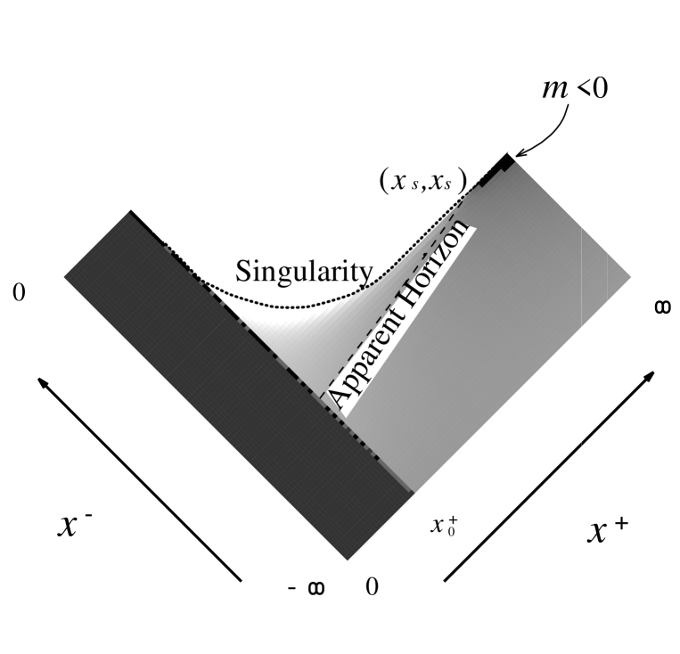
Figure 2: The behavior of the local mass for the RST model in density contour plot, where the density decreases as the local mass grows.

In the region $x^{-}\to-\infty$, the local mass shows the same behavior as that of the original CGHS model. It is clear from the fact that the above RST solutions reduce to the classical ones of the CGHS model at $x^{-}\to-\infty$. On the other hand, the local mass behaves differently at $x^{+}=x^{+}_{0}$ as

$${\cal M}|_{x^{+}=x^{+}_{0}}=M\frac{-\lambda^{2}x^{+}_{0}x^{-}}{-\lambda^{2}x^{+}_{0}x^{-}-N/48}.$$ (3.3)

This difference is caused by the additional effective term (3.1).

The RST model has the advantage that we can evaluate the value of the local mass at $x^{+}=+\infty$ analytically. The information at future null infinity contains that of the end point of the black hole. Also, at future null infinity the local mass directly corresponds to the total energy radiated so far. The result at future null infinity is

$${\cal M}|_{x^{+}\rightarrow+\infty}(x^{-})=M+\frac{N}{48}\Bigl{\{}-\frac{M}{-\lambda^{2}x^{+}_{0}x^{-}}+\lambda\log(1-\frac{M}{-\lambda^{2}x^{+}_{0}x^{-}})\Bigr{\}}.$$ (3.4)

The fact that in the RST model the black hole falls into negative energy state can be reproduced exactly in our study with the local mass. In Ref.[4] it is claimed that up to the point where the singularity and the apparent horizon meet together,

$$x_{s}^{+}=\frac{N\lambda x^{+}_{0}}{48M}(e^{48M/N\lambda}-1),$$

$$x_{s}^{-}=-\frac{M}{\lambda^{3}x^{+}_{0}}\frac{1}{1-e^{-48M/N\lambda}},$$ (3.5)

the total amount of the energy radiated by the Hawking radiation becomes

$$M+\frac{N\lambda}{48}(1-e^{-48M/N\lambda}).$$

This exceeds the energy supplied by the matter shock wave at $x^{+}=x^{+}_{0}$ by $\frac{N\lambda}{48}(1-e^{-48M/N\lambda})$. In fact, the local mass at the future null infinity gives

$${\cal M}(+\infty,x_{s}^{-})=-\frac{N\lambda}{48}(1-e^{-48M/N\lambda}).$$ (3.6)

This confirms the relation between the local mass and the energy momentum tensor (2.15). In Figure 2 one can see the region where the local mass becomes negative at the upper right of $(x_{s}^{+},x_{s}^{-})$.

4. Numerical study of the CGHS model

The equations of motion of the CGHS model at the one-loop level are given by

$$2\left(1-{N\over 12}\,e^{2\phi}\right)\,\partial_{+}\partial_{-}\phi-\left(1-{N\over 24}\,e^{2\phi}\right)\,\left(4\partial_{+}\phi\,\partial_{-}\phi+\lambda^{2}\,e^{2\rho}\right)=0~{},$$

(4.1)

$$\partial_{+}\partial_{-}\phi=\left(1-{N\over 24}\,e^{2\phi}\right)\partial_{+}\partial_{-}\rho~{},$$

where $\rho$ stands for the so-called Liouville field:

$$ds^{2}=-e^{2\rho}dx^{+}dx^{-}~{}.$$

These equations which incorporate the quantum effects are no longer exactly solvable and we shall solve them numerically.

The parameter $\lambda$ can be scaled away and we put $\lambda=1$. The initial data surface, $x^{+}=x_{0}^{+}$, is the line of a shock-wave of an infalling matter and we will choose $x_{0}^{+}=1$. The $\phi$ and $\rho$ on $x^{+}=1$ are those of the linear dilaton vacuum (LDV) and those values are given by

$$\phi(1,x^{-})=\rho(1,x^{-})=-{1\over 2}\,\log\,(-x^{-})~{}.$$ (4.2)

We shall impose boundary conditions at past null infinity such that the solutions become the classical ones there. Actually at a large negative value of $x^{-}$, we impose that the $\phi$ and $\rho$ take the classical values.

For fixed $x^{+}$ the equations (4.1) reduce to the ordinary differential equations for $\partial_{+}\phi$ and $\partial_{+}\rho$ with respect to $x^{-}$. We numerically integrate the equations from a large negative value of $x^{-}$ through the apparent horizon, $\partial_{+}\phi=0$, to the singularity $e^{2\phi}=12/N$. In practice we calculate up to the singularity. With the calculated values of $\partial_{+}\phi$ and $\partial_{+}\rho$ we step forward in the $x^{+}$ direction. Actually the values of $\partial_{+}\phi$ and $\partial_{+}\rho$ on the shock-wave line $x^{+}=1$ can be calculated from Eqs. (4.1) [3, 12],

$$\partial_{+}\phi(1,x^{-}) = -{1\over 2}+{M\over 2}\,\frac{1}{\sqrt{-x^{-}}\,\sqrt{-x^{-}-N/12}}~{},\,$$

$$\partial_{+}\rho(1,x^{-}) = -{1\over 2}-{12\,M\over N}\,\left(1-\sqrt{1+{N\over{12\,x^{-}}}}^{-1}\right)~{}.$$

and they can be used to check the accuracy of the numerical algorithm. The numerical method which we adopted is explained in the appendix.

The result of the singularity and the apparent horizon in the CGHS model for $M=25$ and $N=600$ is shown in Fig. 3. It indicates that the singularity and the apparent horizon meet at finite $x^{+}$ and $x^{-}$ which we denote $(x^{+}_{EP},x^{-}_{EP})$.

Figure 3: The singularity and the apparent horizon in the CGSH model.

The local mass function (2.6) in the CGHS model for the same $M$ and $N$ is shown in Fig. 4 and 5.

CGHSmassa.eps

Figure 4: The local mass function in the CGSH model (3Dplot).

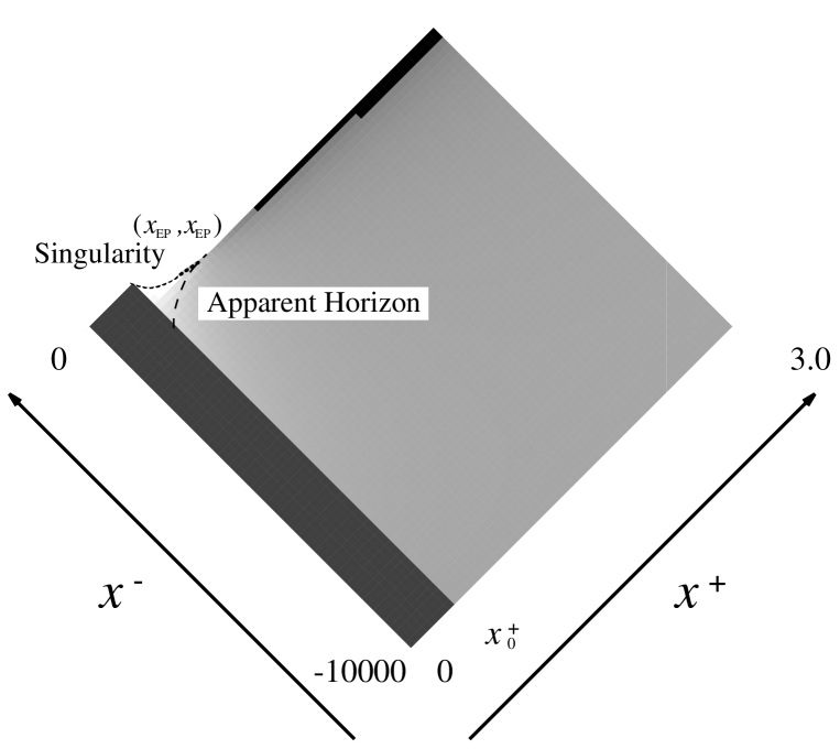
Figure 5: The local mass function in the CGSH model (density plot).

The figure 5 shows that the local mass becomes negative in some region, before $x^{-}=x^{-}_{EP}$ in the $x^{-}$ direction and after the endpoint $x^{+}>x^{+}_{EP}+({\rm some\ const.})$ in the $x^{+}$ direction, in a manner similar to the RST model.

5. Discussion

In the previous section we found that the amount of the Hawking radiation in the CGHS model exceeds the incoming energy as was seen in the RST model case. In other words, the CGHS model fails to end up as the vacuum but evolves into a space-time whose scalar curvature is negative.

One interpretation is that this merely means the failure of the CGHS model as a toy model for four dimensional black hole models. Note in particular that we have coupled scalar matter fields to the gravitational field in a way that is different from the four dimensional case. This coupling of the matter fields enables us to calculate the back reaction but could also cause the excess of the radiation energy.

One possible modification of the CGHS model may come from string theory. There have been many attempts to resolve the problems associated with black holes by applying string theory and one approach along this line is the following. The term $(1/4)e^{-2\phi}\alpha^{\prime}R_{abcd}R^{abcd}$[19], where $\alpha^{\prime}$ is the inverse of the string tension, will provide string corrections to the model. It would be interesting to estimate the effect of this using present local mass analysis.

For further investigation it may also be interesting to analyze a black hole model proposed by Nojiri and Oda [20]. The model is described by SL(2,R)/U(1) gauged WZW model deformed by (1,1) operator and they claim that the black hole reaches a zero mass state and evaporates completely.

Acknowledgment We would like to thank T. Eguchi for suggestive discussion. One of the authors (T.T) would like to thank Soryuushi Shougakukai for the financial support at the early stage of the present work. His thanks are also due to ITP members for their hospitality and the participants of the conference ‘Quantum Aspects of Black Holes’, especially to A. Strominger for discussions. Finally useful comments by D. Marolf to the manuscript is gratefully acknowledged.

A. The Numerical Method

The two dimensional surface $(x^{+},x^{-})$ is represented by a two dimensional lattice with equal spacing in each direction. The lattice spacing in the $x^{+}$ direction is much narrower than that in the $x^{-}$ direction.

The equation (4.1) can be symbolically represented by

$$\partial_{-}\partial_{+}\phi = f(\phi,\rho,\partial_{+}\phi)~{},$$

$$\partial_{-}\partial_{+}\rho = g(\phi)\,\partial_{-}\partial_{+}\phi~{}.$$

and for fixed $x^{+}$ the first equation can be seen as an ordinary differential equation of the first order for $\partial_{+}\phi$. We use the fourth-order Runge-Kutta method to get $\partial_{+}\phi$ in the $x^{-}$ direction. We have adopted the “Cubic Spline Interpolation” method to get values of an arbitrary $x^{-}$ at fixed $x^{+}$ and $\partial_{-}\phi$ and $\partial_{-}\rho$ are computed with a fourth-order backward differential method.

The values of $\phi$ and $\rho$ on the next $x^{+}={\rm const.}$ line are obtained from $\partial_{+}\phi$ and $\partial_{+}\rho$ by linear extrapolation.

References

- [1] C.G. Callan, S.B. Giddings, J.A. Harvey and A. Strominger, Phys. Rev. D45 (1992) R1005.
- [2] T. Banks, A. Dabholkar, M.R. Douglas and M. O’Loughlin, Phys. Rev. D45 (1992) 3607.
- [3] J.G. Russo. L. Susskind and L. Thorlacius, Phys. Lett. B292 (1992) 13
- [4] J.G. Russo. L. Susskind and L. Thorlacius, Phys. Rev. D46 (1992) 3444; ibid. D47 (1993) 533.
- [5] A. Biral and C. Callan, Nucl. Phys. B394 (1993) 73.
- [6] A. Strominger, Phys. Rev. D46 (1992) 4396.
- [7] S.P. de Alwis, Phys. Lett. B289 (1992) 278; ibid. B300(1993) 330.
- [8] K. Hamada, Phys. Lett. B300 (1993) 322.
- [9] S.W. Hawking and J. M. Stewart, Nucl. Phys. B400 (1993) 393.
- [10] David A. Lowe, Phys. Rev. D47(1993) 2446.
- [11] Tsvi Piran and Andrew Strominger, Phys. Rev. D48 (1993) 4729.
- [12] T. Tada and S. Uehara, Phys. Lett. B305 (1993) 23
- [13] W. Fischler, D. Morgan and J. Polchinski, Phys. Rev. D42 (1990) 4042.
- [14] A. Tomimatsu, Phys. Lett. B289 (1992) 283.
- [15] M. D. McGuigan, C.R. Nappi and S. A. Yost, Nucl. Phys. B375 (1992) 421
- [16] V. P. Frolov, Phys. Rev. D46 (1992) 5383
- [17] R. Mann, Phys. Rev. D47 (1993) 4438.
- [18] H. Kodama, Prog. Theor. Phys. 63 (1980) 1217.
- [19] C. G. Callan, R. C. Myers and M. J. Perry, Nucl. Phys. 311 (1988/89) 673.
- [20] S. Nojiri and I. Oda, preprint NDA-FP-10-93, hepth@xxx/9302024 (1993); Phys. Rev. D49 (1994) 4066.