DTP-94-35

September 1994

hep-th/9409035

On the Breathers of

$a_{n}^{(1)}$ Affine Toda Field Theory

Uli Harder, Alexander A. Iskandar, William A. McGhee

Department of Mathematical Sciences,

University of Durham,

Durham DH1 3LE,

England.

Abstract

Explicit constructions of $a_{n}^{(1)}$ affine Toda field theory breather solutions are presented. Breathers arise either from two solitons of the same species or from solitons which are anti-species of each other. In the first case, breathers carry topological charges. These topological charges lie in the tensor product representation of the fundamental representations associated with the topological charges of the constituent solitons. In the second case, breathers have zero topological charge. The breather masses are, as expected, less than the sum of the masses of the constituent solitons.

1 Introduction

Toda field theories have attracted interest for various reasons over the past few decades [1, 2, 3]. Of particular interest is the affine Toda field theory which is a perturbed conformal field theory that is still integrable [4]. There has been much progress in the understanding of the real coupling regime of these affine Toda theories [5, 6, 7, 8, 9, 10, 11].

More recently, Hollowood [12] showed that the $a_{n}^{(1)}$ series of affine Toda field theories have complex soliton solutions with real energy. The reality of energy and momentum has been generalized by Olive et al. to include all affine Toda theories associated with the affine Kac-Moody algebras [13, 14]. The sine-Gordon theory is the simplest example of the $a_{n}^{(1)}$ series, i.e. the $a^{(1)}_{1}$ Toda field theory. Besides soliton and antisoliton solutions of the sine-Gordon theory, there also exist oscillating solitonic solutions, the breathers. These breathers are bound states of the sine-Gordon soliton and antisoliton pair. Since the $a_{n}^{(1)}$ affine Toda field theory is a generalization of the sine-Gordon theory, it is natural to ask if such breather solutions also exist for these theories. Much has been conjectured about the breathers of the affine Toda field theory [12, 13, 14, 15]. Calculation of the scattering processes of the $a_{n}^{(1)}$ affine Toda solitons [16] also points to the existence of these breathers, since there are poles in the soliton $S$-matrix which correspond to bound states of soliton pairs. However, an explicit construction is lacking. The motivation behind this work is to give an explicit expression of classical breather solutions for the $a_{n}^{(1)}$ affine Toda field theory based on a similar construction to that of the sine-Gordon breather.

The affine Toda field theory Lagrangian density is given by,

$${\cal L}=\frac{1}{2}(\partial_{\mu}\phi)(\partial^{\mu}\phi)-\frac{m^{2}}{\tilde{\beta}^{2}}\sum_{j=0}^{n}n_{j}(e^{\tilde{\beta}\alpha_{j}\cdot\phi}-1),$$ (1.1)

where $\phi$ is an $n$-dimensional scalar field, $m$ and $\tilde{\beta}$ are the mass and coupling parameters respectively. The vectors $\alpha_{j}$ with $j=1,2,\ldots,n$ are the simple roots of the Lie algebra $g$ of rank $n$ associated with the theory. And $\alpha_{0}$ is chosen such that the set $\{\alpha_{0},\alpha_{j}\}$ represents the affine Dynkin diagram of an affine Kac-Moody algebras. For the simply-laced Kac-Moody algebras, $\alpha_{0}$ is the negative of the highest root $\psi=\sum_{j=1}^{n}n_{j}\alpha_{j}$; in particular, for the $a_{n}^{(1)}$ series, $n_{j}=1$ for all $j$. The constants $n_{j}$ are inserted into the potential term so that $\phi=0$ is a vacuum solution.

Substituting the coupling parameter $\tilde{\beta}$ with a purely imaginary coupling parameter, $i\beta$, the affine Toda field theory potential admits multiple vacua. The existence of these vacua signals a possibility of topological solitonic solutions which interpolate between them. The equation of motion can be derived easily from (1.1) upon substitution of the purely imaginary coupling parameter,

$$\partial^{2}\phi=-\frac{m^{2}}{i\beta}\sum_{j=0}^{n}n_{j}\alpha_{j}\exp(i\beta\alpha_{j}\cdot\phi).$$ (1.2)

Soliton solutions have been calculated using the Hirota’s methods [12, 19], and using an algebraic method [13, 14]. This algebraic approach is a generalization of the Leznov-Saveliev solution of the conformal Toda theory [17] where the simplest affine case, i.e. the sine-Gordon theory, has been discussed by Mansfield [18].

For the $a^{(1)}_{1}$ Toda field theory, which is the sine-Gordon theory, the single soliton solution is given by,

$$\phi=\frac{i\sqrt{2}}{\beta}\ln\left(\frac{1-e^{\sigma(x-vt)+\rho}}{1+e^{\sigma(x-vt)+\rho}}\right),$$ (1.3)

with the constraint $\sigma^{2}(1-v^{2})=4m^{2}$. The parameter $\rho=\eta+i\xi$ is complex, and its imaginary part determines the topological charge of the soliton. In this case, there are two possibilities, the soliton and the antisoliton, which have the same mass equal to $\frac{8m}{\beta^{2}}$. It is well known (see for instance Rajaraman [21]) that beside these soliton solutions, there also exist oscillating solitonic solutions, or breathers. The sine-Gordon breather is constructed from two approaching soliton solutions by changing the velocity $v$ into $iv$,

$$\phi_{\it breather}=\frac{i\sqrt{2}}{\beta}\ln\left(\frac{1-e^{\sigma(x-ivt)+\rho_{1}}-e^{\sigma(x+ivt)+\rho_{2}}-v^{2}e^{2\sigma x+(\rho_{1}+\rho_{2})}}{1+e^{\sigma(x-ivt)+\rho_{1}}+e^{\sigma(x+ivt)+\rho_{2}}-v^{2}e^{2\sigma x+(\rho_{1}+\rho_{2})}}\right).$$ (1.4)

Taking $\xi_{1}=-\xi_{2}=-\frac{\pi}{2}$ and $\eta_{1}=\eta_{2}=\eta$, yields a soliton solution oscillating about the point $\frac{\ln(v^{2})+2\eta}{2\sigma}$. As it is constructed from a soliton-antisoliton pair, this sine-Gordon breather has zero topological charge; its mass is equal to $\frac{16m}{\beta^{2}\sqrt{1+v^{2}}}$.

Following the prescription of taking imaginary velocity, the breathers created from two solitons of the $a_{n}^{(1)}$ affine Toda theories can be constructed. It turns out that in order for the energy of the breathers built from two solitons to be real, the constituent solitons must be of the same mass and approaching each other with the same imaginary velocity, resulting in a stationary breather. To obtain a moving breather, one can apply the usual Lorentz boost to the breather solution. The condition of real energy also produces an expression for the masses of these breathers which is less than the sum of the constituent solitons. One type of breathers can carry topological charge which coincides with the topological charge of a certain single soliton, while the other type has zero topological charge.

This paper is organised as follows. As breather solutions are constructed from soliton solutions, section two discusses the soliton solutions of the $a_{n}^{(1)}$ series. In section three, the breathers created from two solitons of the $a_{n}^{(1)}$ series are determined, and it is shown that there are two types. Type A breathers are constructed from two solitons of the same species and type B breathers are constructed from two solitons of opposite species. The type A breathers carry topological charge while type B breathers have zero topological charge, these will be discussed in section four together with some properties of the breather solution. It will be shown also that these topological charges lie in a fundamental representation which is a subset of a tensor product representation of the fundamental representations which are associated to the topological charges of the constituent solitons. Section five will discuss the sine-Gordon embedding in some cases of the $a_{n}^{(1)}$ family. Examples of the $a_{3}^{(1)}$ and $a_{4}^{(1)}$ breathers are given in section six. Section seven contains concluding remarks.

2 Soliton Solutions

This section provides a review on the construction of soliton solutions for the $a_{n}^{(1)}$ affine Toda field theory [12, 19]. Soliton solutions to the affine Toda equation of motion, (1.2), can be derived using Hirota’s method. An ansatz for the soliton solutions of the $a_{n}^{(1)}$ affine Toda field theory [12] is the following,

$$\phi=\frac{i}{\beta}\sum_{j=1}^{n}\alpha_{j}\ln\frac{\tau_{j}}{\tau_{0}}.$$ (2.1)

In Hirota’s method [22], the $\tau$-functions are a power series expansion in an arbitrary parameter $\varepsilon$ which will be set to 1 at the end of the construction,

$$\tau_{j}=1+\varepsilon t^{(1)}_{j}+\varepsilon^{2}t^{(2)}_{j}+\dots.$$ (2.2)

In the above expression, $t_{j}$ is a function of $(x,t)$. The equation of motion is solved order by order in the arbitrary parameter $\varepsilon$. An $N$ soliton solution is calculated by setting $t^{(a)}_{j}=0$ for $a>N$.

Inserting the ansatz (2.1) into the equation of motion (1.2), and assuming that the set of $h=n+1$ equations of motion decouple, results in the following,

$${\ddot{\tau_{j}}}\tau_{j}-{\dot{\tau_{j}}}^{2}-\tau_{j}^{\prime\prime}\tau_{j}+\tau_{j}^{\prime 2}=m^{2}(\tau_{j-1}\tau_{j+1}-\tau_{j}^{2})\qquad j=0,1,\ldots,n,$$ (2.3)

where the subscripts of the $\tau$-functions are labelled modulo the Coxeter number $h=n+1$. A single soliton solution is obtained by keeping the $\tau$-function expansion up to the order $\varepsilon$ and inserting to the above equation of motion. This yields,

$$\tau^{(a)}_{j}=1+\exp[\Omega_{a}+\rho_{a}+ij\theta_{a}]$$ (2.4)

where,

$$\Omega_{a}=\sigma_{a}(x-u_{a}t),\qquad\rho_{a}=\eta_{a}+i\xi_{a},\qquad\theta_{a}=\frac{2\pi a}{h},$$ (2.5)

$\sigma_{a},u_{a},\eta_{a},\xi_{a}$ $\in$ IR. The parameter $\sigma_{a}$ and the velocity $u_{a}$ are related by,

$$\sigma_{a}^{2}(1-u_{a}^{2})=4m^{2}\sin^{2}\frac{\pi a}{h}.$$ (2.6)

The superscript $a$ of the $\tau$-function (2.4) indicates the species of the soliton, which can take the value $1\leq a\leq n$. One can also write the $\tau$-functions with an explicit dependence on the lightcone coordinates, $x_{\pm}=\frac{1}{\sqrt{2}}(t\pm x)$, then $\Omega_{a}$ becomes,

$$\Omega_{a}=\delta_{a}^{(-)}x_{+}-\delta_{a}^{(+)}x_{-},$$

with,

$$\delta_{a}^{(\pm)}=\frac{1}{\sqrt{2}}\sigma_{a}(1\pm u_{a}).$$

A two soliton solution is obtained by solving the equation of motion (2.3) after inserting the expansion of the $\tau$-function up to second order in $\varepsilon$. The two soliton solution for species $a$ and $b$ is,

$$\tau^{(ab)}_{j} = 1+\exp[\Omega_{a}+\rho_{a}+ij\theta_{a}]+\exp[\Omega_{b}+\rho_{b}+ij\theta_{b}]$$ (2.7)

$$+A\exp[\Omega_{a}+\Omega_{b}+\rho_{a}+\rho_{b}+ij(\theta_{a}+\theta_{b})]$$

which can be compactly written as,

$$\tau^{(ab)}_{j}=1+(\tau^{(a)}_{j}-1)+(\tau^{(b)}_{j}-1)+A(\tau^{(a)}_{j}-1)(\tau^{(b)}_{j}-1).$$ (2.8)

The interaction coefficient in the above expression is given by,

$$A=-\frac{(\sigma_{a}-\sigma_{b})^{2}-(\sigma_{a}u_{a}-\sigma_{b}u_{b})^{2}-4m^{2}\sin^{2}(\frac{\pi}{h}(a-b))}{(\sigma_{a}+\sigma_{b})^{2}-(\sigma_{a}u_{a}+\sigma_{b}u_{b})^{2}-4m^{2}\sin^{2}(\frac{\pi}{h}(a+b))}.$$ (2.9)

If the rapidity variable $\Theta_{a}$ is defined through the velocity $u_{a}$ as, $u_{a}=\tanh\Theta_{a}$, then the interaction coefficient can be written in terms of rapidity difference $\Theta=\Theta_{a}-\Theta_{b}$ as,

$$A=\frac{\sin\left(\frac{\Theta}{2i}+\frac{\pi(a-b)}{2h}\right)\sin\left(\frac{\Theta}{2i}-\frac{\pi(a-b)}{2h}\right)}{\sin\left(\frac{\Theta}{2i}+\frac{\pi(a+b)}{2h}\right)\sin\left(\frac{\Theta}{2i}-\frac{\pi(a+b)}{2h}\right)}.$$ (2.10)

As in the case for two soliton solutions, a multi-soliton solution can be constructed from a collection of single soliton solutions [12]. The interaction between the solitons is pair-wise with the interaction coefficient as given above.

The energy-momentum tensor of soliton solutions can be written as [13],

$$T_{\mu\nu}=(\eta_{\mu\nu}\partial^{2}-\partial_{\mu}\partial_{\nu})C.$$ (2.11)

Or in terms of the lightcone components,

$$T_{+-} = \partial_{+}\partial_{-}C,$$ (2.12)

$$T_{\pm\pm} = -\partial_{\pm}^{2}C.$$ (2.13)

$T_{+-}$ is actually the trace of the energy-momentum tensor, then (2.12) becomes,

$$\partial^{2}C=-\frac{2m^{2}}{\beta^{2}}\sum_{j=0}^{n}\left(e^{i\beta\alpha_{j}\cdot\phi}-1\right).$$ (2.14)

Using the soliton solutions in the energy-momentum tensor leads to the following solution for the function $C$ up to a constant,

$$C=-\frac{2}{\beta^{2}}\sum_{j=0}^{n}\ln\tau_{j}.$$ (2.15)

The mass of the soliton solution can be calculated as follows. The energy and momentum density is given in terms of components of the energy-momentum density as, ${\cal E}=T_{00}$ and ${\cal P}=T_{10}$. Consider instead, the lightcone energy-momentum density,

$${\cal P^{\pm}}=\frac{{\cal E\pm P}}{\sqrt{2}},$$ (2.16)

Thus, using (2.11), the components of the lightcone energy-momentum are given by,

$$P^{+}=(-\partial_{+}C)_{x=-\infty}^{\infty},\qquad\qquad P^{-}=(\partial_{-}C)_{x=-\infty}^{\infty}.$$ (2.17)

For the single soliton solution (2.4), one finds that

$$\partial_{\pm}C=\mp\frac{2}{\beta^{2}}\sum_{j=0}^{n}\frac{\delta_{a}^{\mp}(\tau_{j}^{(a)}-1)}{\tau_{j}^{(a)}},$$ (2.18)

In the limit as $x\rightarrow-\infty$ the ratios $\frac{(\tau_{j}^{(a)}-1)}{\tau_{j}^{(a)}}$ vanish, and in the limit $x\rightarrow\infty$ all the ratios tend to 1. Recall the constraint (2.6) and write the rapidity of the soliton as $\Theta_{a}=\frac{1}{2}\ln\left(\frac{1+u_{a}}{1-u_{a}}\right)$, then the lightcone energy-momentum of a single soliton is given by

$$P^{\pm}=\frac{4hm}{\sqrt{2}\beta^{2}}\sin\left(\frac{\theta_{a}}{2}\right)e^{\mp\Theta_{a}}$$ (2.19)

And its mass is calculated to be

$$M_{a}^{2}=2P^{+}P^{-}=\left(\frac{4hm}{\beta^{2}}\sin\left(\frac{\theta_{a}}{2}\right)\right)^{2}.$$ (2.20)

Note, that the mass of the species $a$ soliton is proportional to the mass of the fundamental particle of the $a_{n}^{(1)}$ affine Toda field theory, $m_{a}=2m\sin(\frac{\theta_{a}}{2})$.

For a multi-soliton solution the calculation above can be performed in the same way. In particular a two soliton solution of species $a$ and $b$ yields,

$$\sqrt{2}P^{\pm}=M_{a}e^{\mp\Theta_{a}}+M_{b}e^{\mp\Theta_{b}}.$$ (2.21)

The single solitons of species $a$ carry topological charges which lie in the highest weight representation of the $a^{th}$ fundamental weight of the $A_{n}$ Lie algebra [24]. Thus, it is natural to associate the species of the solitons with the nodes of the Dynkin diagram of the associated Lie algebra, $A_{n}$.

3 Breather Solutions

To obtain an oscillating solitonic solution which is constructed from two solitons, one can follow the sine-Gordon prescription of changing the velocity into an imaginary velocity, i.e. changing $u$ into $iv$ in the $\tau$-functions. Care must be taken in the analytic continuation of $u\rightarrow iv$ such that the energy and momentum are real, although the energy and momentum densities generally are complex.

Changing $u$ into $iv$ also means changing a real rapidity into an imaginary rapidity, with a relation between velocity $v$ and rapidity $\Theta$ becomes $v=\tan(-i\Theta)$. From the lightcone energy-momentum of the two soliton solution (2.21), a real energy and momentum can be achieved provided that the two solitons forming a breather are of the same mass and moving towards to each other with the same velocity giving a stationary breather. One can make an oscillating solution from solitons of two different masses, but the energy and momentum of this solution will not be real. Generally, one can add a real rapidity $\Theta_{0}$ as a phase in the energy-momentum tensor, which acts as a Lorentz boost to the breather solution. Thus,

$$P^{\pm}_{breather}=\frac{4hm_{a}}{\sqrt{2}\beta^{2}}\cos(\Theta_{a})e^{\mp\Theta_{0}},$$ (3.1)

$m_{a}$ above is the mass of the fundamental particles of the $a_{n}^{(1)}$ affine Toda theory. For simplicity, in what follows only stationary breathers are considered. Hence (3.1) becomes,

$$P^{\pm}_{breather}=\frac{4h}{\sqrt{2}\beta^{2}}\frac{m_{a}}{\sqrt{1+v^{2}}},$$ (3.2)

and the mass of a breather is,

$$M_{breather}=\frac{2M_{a}}{\sqrt{1+v^{2}}}=\frac{4hm_{a}}{\beta^{2}\sqrt{1+v^{2}}}.$$ (3.3)

It is obvious that the mass of a breather is less than the sum of its constituent solitons. This result generalizes the sine-Gordon case, i.e. taking $h=2$ gives the mass of the sine-Gordon breather.

The masses $m_{a}$ of the fundamental particles of $a_{n}^{(1)}$ series are degenerate with respect to the $Z_{2}$ symmetry of the $A_{n}$ Dynkin diagram, i.e. $m_{a}=m_{h-a}$. Hence, there are two possibilities of forming a breather. Either the two constituent solitons are of the same species, these breathers will be called type A breathers or, the two constituent solitons are of opposite species, type B breathers. Exceptions to this classification are the breathers constructed from solitons of species $(n+1)$ of the $a_{2n+1}^{(1)}$ theories. These breathers are sine-Gordon embedded breathers which belong to both type A and B as will be explained in the following sections.

Looking back at the $\tau$-function of a two soliton solution of the same constituent mass, choosing $u_{a}=-u_{b}=iv$ yields the breather $\tau$-function,

$$\tau^{(ab)}_{j} = 1+\exp[\sigma_{a}(x-ivt)+\rho_{a}+ij\theta_{a}]+\exp[\sigma_{b}(x+ivt)+\rho_{b}+ij\theta_{b}]$$ (3.4)

$$+\exp[\sigma_{+}x+\lambda+\rho_{+}+ij\theta_{+}],$$

the interaction coefficient is written as $A=e^{\lambda}$ with $\lambda=\zeta+i\delta$, where $\zeta,\delta$ $\in$ IR and

$$\sigma_{+}=\sigma_{a}+\sigma_{b},\qquad\rho_{+}=\rho_{a}+\rho_{b},\qquad\theta_{+}=\theta_{a}+\theta_{b},$$

$$\eta_{-}=\eta_{a}-\eta_{b},\qquad\xi_{+}=\xi_{a}+\xi_{b}.$$

Note that for solitons of the same mass, $\sigma_{a}=\sigma_{b}$. By the ansatz (2.1), it is clear that in order to have a well-defined solution, each $\alpha_{j}$ component of the solution $\phi$ must be well defined. Thus, for each $j$, the ratio $\frac{\tau_{j}}{\tau_{0}}$ must not become zero or infinite. Evaluation of the behaviour of the $\tau$-function can be done easily by writing the real and imaginary part of (3.4) explicitly. It turns out that to avoid the real and imaginary part of (3.4) becoming zero simultaneously at the same point, the parameters $\xi_{+}$ and $\eta_{-}$ are restricted to a certain range of definition.

Moreover, for type A and B breathers, the interaction coefficient can have either positive or negative value. The critical velocity when the interaction coefficient changes sign is, for a type A breather

$$v^{(A)}_{c}=\tan(\frac{\theta_{a}}{2}),$$ (3.5)

and for a type B breather,

$$v^{(B)}_{c}=\frac{1}{v^{(A)}_{c}}.$$ (3.6)

For breathers with constituent solitons of species $a=\frac{h}{2}$, the interaction coefficient never changes sign.

3.1 Type A Breathers

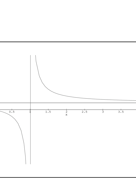
Figure 1: The graph shows the behaviour of the interaction coefficient for the type A breather solution. The interaction $A^{\prime}$ is given by $A^{\prime}=A\cos(\theta/2)$, the velocity as $x=v^{2}/v^{2}_{c}$. As mentioned in section 3.1 there is an upper bound for the velocity. This has not been marked in the graph.

The breathers with constituent solitons of the same species will have a negative interaction coefficient, $A<0$, when $v^{2}<v^{(A)2}_{c}$ (see figure 1). For these breathers, both the real and imaginary part of (3.4) will be trivially zero when the parameters $\xi_{+}$ have the following values,

$$\xi_{+}=(2\pi-j\theta_{+})\mbox{ mod }2\pi,\qquad j=0,\ldots,n.$$ (3.7)

This divides the range of $\xi_{+}$ into several regions which will determine the topological charge of the breather.

Furthermore, the maximum “distance” of separation between the two constituent solitons is restricted as follows,

$$-\min_{j}(\eta^{j}_{c})<\eta_{-}<\min_{j}(\eta^{j}_{c}),$$

where,

$$\eta^{j}_{c}=\mbox{arcosh}\left[2|A|\sin^{2}\frac{1}{2}(\xi_{+}+j\theta_{+})+1\right],$$

with $j=0,\ldots,n$. Each $\eta^{j}_{c}$ above will restrict $\tau_{j}$ such that it will never be zero. Hence, for all $\tau$-functions to avoid zero, the minimum value of $\eta^{j}_{c}$ is taken as the limit on the range of $\eta_{-}$.

For breathers of type A with positive interaction coefficient, the parameters $\xi_{+}$ must not have the following values,

$$\xi_{+}=(\pi-j\theta_{+})\mbox{ mod }2\pi,\qquad j=0,\ldots,n.$$ (3.8)

The separation “distance” is restricted as above with,

$$\eta^{j}_{c}=\mbox{arcosh}\left[2A\cos^{2}\frac{1}{2}(\xi_{+}+j\theta_{+})-1\right].$$

As $\eta^{j}_{c}$ are defined through an arcosh-function, these $\eta^{j}_{c}$ in turn will restrict the allowed velocity of the constituent solitons. Generally, not all $v^{2}>v^{(A)2}_{c}$ are allowed. In fact all velocities with absolute value greater than the absolute value of the critical velocity are allowed if for all $j$ the following is true,

$$\left[1-\frac{\cos^{2}\frac{1}{2}(\xi_{+}+j\theta_{+})}{\cos^{2}(\frac{\theta_{+}}{4})}\right]<0.$$

Otherwise, the velocity is bounded from above by,

$$v^{(A)2}_{c}<v^{2}\leq\frac{v^{(A)2}_{c}}{{\displaystyle\max_{j}}\left[1-\frac{\cos^{2}\frac{1}{2}(\xi_{+}+j\theta_{+})}{\cos^{2}(\frac{\theta_{+}}{4})}\right]}.$$

3.2 Type B Breathers

The constituent solitons of type B breathers are of opposite species. The negative interaction coefficient regime is accomplished with $v^{2}>v^{(B)2}_{c}$. In this case, the real and imaginary part of the $\tau$-functions will be trivially zero for

$$\xi_{+}=0\mbox{ mod }2\pi,$$ (3.9)

i.e. the parameter $\xi_{+}$ must not be an integer multiple of $2\pi$. For each $\tau_{j}$ to avoid zero, the separation parameter $\eta_{-}$ is limited to take values between,

$$-\min_{j}(\eta^{j}_{c})<\eta_{-}<\min_{j}(\eta^{j}_{c}),$$

where,

$$\eta^{j}_{c}=\mbox{arcosh}\left[2|A|\sin^{2}\frac{1}{2}(\xi_{+}+j\theta_{+})+1\right],$$

with $j=0,\ldots,n$. As for type A breathers, each $\tau_{j}$ has its own $\eta^{j}_{c}$, and the smallest of these is taken as the limit.

Contrary to the type A breathers, it is not possible to have type B breathers with positive interaction coefficient, or to have velocity $v^{2}<v^{(B)2}_{c}$. Since the $\tau$-functions would necessarily pass the origin and this would lead to a solution which is not well-defined.

4 Properties of the Breather Solutions

4.1 The Interaction Coefficient

The interaction coefficient A has properties similar to the properties of the $S$-matrix of the fundamental Toda particles. Recall the expressions for A from (2.9) and (2.10). The interaction term of the type A breathers is,

$$A_{aa}=\frac{v^{2}}{(1+v^{2})\cos^{2}(\frac{\theta_{a}}{2})-1},$$ (4.1)

or in terms of rapidity difference $i\Theta$,

$$A_{aa}=\frac{\sin^{2}(\frac{i\Theta}{2})}{\sin(\frac{i\Theta}{2}+\frac{\theta_{a}}{2})\sin(\frac{i\Theta}{2}-\frac{\theta_{a}}{2})}.$$ (4.2)

And for type B breathers,

$$A_{a{\bar{a}}}=(1+v^{2})\cos^{2}(\frac{\theta_{a}}{2})-v^{2},$$ (4.3)

in terms of rapidity difference $i\Theta$,

$$A_{a{\bar{a}}}=\frac{\cos(\frac{i\Theta}{2}+\frac{\theta_{a}}{2})\cos(\frac{i\Theta}{2}-\frac{\theta_{a}}{2})}{\cos^{2}(\frac{i\Theta}{2})}.$$ (4.4)

As the case of $S$-matrices of fundamental Toda particles, these interaction coefficients admit a pole. For type A breathers,

$$v=v^{(A)}_{c}\qquad\mbox{ or, }\qquad i\Theta=\frac{2\pi a}{h}$$ (4.5)

and, for type B breathers,

$$v\rightarrow\infty\qquad\mbox{ or, }\qquad i\Theta=\pi.$$ (4.6)

It is readily seen that the pole of $A_{aa}$ is exactly the fusing angle related to the process $a+a\rightarrow{\overline{(h-2a)}}$ of the fundamental particles [5]. Hollowood noted that the same fusing rule also applies to soliton fusings in $a_{n}^{(1)}$ theories [12]. In fact, the fusing rule of fundamental particles applies also to all simply laced affine Toda solitons [13, 23]. The fusing of two solitons of species $a$ into ${\overline{(h-2a)}}$ hinted that the topological charge of type A breathers has to be found in the same representation as the topological charges of ${\overline{(h-2a)}}$ single solitons.

It is not surprising that at the pole of the interaction coefficient, the breathers fail to exist. Using the breather $\tau$-function, (3.4), with the interaction coefficient approaching its pole, the interaction term dominates. Hence, the solution falls into one of the vacuum solutions of the complex affine Toda potential,

$$\phi=-\frac{1}{\beta}\sum^{n}_{j=1}j\alpha_{j}\theta_{+}.$$ (4.7)

On the other hand, if the positions of the constituent solitons are simultaneously shifted by $-\frac{\zeta}{2}$, i.e. changing $\eta\rightarrow\eta-\frac{\zeta}{2}$, the breather turns into a static solution as the interaction coefficient approaches its pole.

When there is no interaction between the constituent solitons, the interaction coefficient is zero. In this case, the $\tau$-functions do not give a well defined solution, as the $\tau$-functions will vanish at a particular point in space-time. This is quite obvious, since the breathers are bound states of soliton pairs and therefore a breather interaction coefficient cannot be zero.

Furthermore, the interaction coefficient $A$ has the following general properties some of which are similar but not the same as the properties of the $S$-matrix,

• Crossing symmetry

  $$A_{aa}(v)=A^{-1}_{a{\bar{a}}}(\frac{1}{v})\qquad\mbox{ or, }\qquad A_{aa}(i\Theta)=A^{-1}_{a{\bar{a}}}(i\Theta-\pi).$$ (4.8)

• Evenness

  $$A(v)=A(-v)\qquad\mbox{ or, }\qquad A(i\Theta)=A(-i\Theta).$$ (4.9)

• Symmetry

  $$A_{a{\bar{a}}}(v)=A_{{\bar{a}}a}(v)\qquad\mbox{ or, }\qquad A_{a{\bar{a}}}(i\Theta)=A_{{\bar{a}}a}(i\Theta).$$ (4.10)

• Periodicity

  $$A(i\Theta)=A(i\Theta+2\pi).$$ (4.11)

4.2 The Topological Charges

In the soliton solutions of the complex affine Toda field equations, the topological charge is a conserved quantity of zero spin. For the $a_{n}^{(1)}$ series, topological charges of the single and multi-soliton solutions have been calculated [24]. Unfortunately, the calculation of topological charges of multi-soliton solutions used there is not applicable for breathers because the two solitons constituting the breather only separate a finite “distance” from each other.

The topological charge $q$ of a solution $\phi$ is defined by

$$q=\frac{\beta}{2\pi}\int_{-\infty}^{\infty}\partial_{x}\phi\mbox{d}x=\frac{\beta}{2\pi}\lim_{x\to\infty}(\phi(x,t)-\phi(-x,t)).$$ (4.12)

Writing the solution $\phi$ in terms of the breather $\tau$-functions, defining $f_{j}=\frac{\tau_{j}}{\tau_{0}}$ for $j=1\dots n$ and making use of the definition of the logarithm of a complex number, (4.12) can be recast as

$$q=-\frac{1}{2\pi i}\sum_{j=1}^{n} \alpha_{j} \;\lim_{x\to\infty}\{\ln|f_{j}(x,t)|-\ln|f_{j}(-x,t)|$$ (4.13)

$$+ i\arg(f_{j}(x,t))+2i\pi k^{\prime}-i\arg(f_{j}(-x,t))-2i\pi k^{\prime\prime}\},$$

where $k^{\prime},k^{\prime\prime}\in\mbox{\sf ZZ}$. A simplification of (4.13) results from the fact that $\lim_{|x|\to\infty}|f_{j}(x,t)|=1$, thus

$$q=-\frac{1}{2\pi}\sum_{j=1}^{n}\alpha_{j}\;\lim_{x\to\infty}\{\arg(f_{j}(x,t))-\arg(f_{j}(-x,t))+2\pi k\}$$ (4.14)

with $k=k^{\prime}-k^{\prime\prime}$. The number $k$ determines the curve $f_{j}$ in the complex plane, and in particular, how often and in what direction it winds around the origin. The topological charge is therefore determined by the change in the argument of $f_{j}$ as $|x|$ goes to infinity.

For the type A breather it is not too difficult to deduce the number of distinct topological charges in the fashion of [24]. The number of the topological charges is determined by the number of sectors of allowed values of $\xi_{+}$. From the expression for forbidden $\xi_{+}$’s, (3.7) or (3.8), it follows that one looks for the smallest number $p$ for which

$$\frac{2ap}{h}=k\,\mbox{with}\,p,k\in\mbox{\sf IN}.$$ (4.15)

Here $a$ is the species of the constituent solitons and $h$ is the Coxeter number.

With $2\tilde{a}=\frac{2a}{\gcd(2a,h)}$, $\tilde{h}=\frac{h}{\gcd(2a,h)}$ then (4.15) can be rewritten as

$$2\tilde{a}p=\tilde{h}k.$$ (4.16)

Because $2\tilde{a}$ and $\tilde{h}$ are coprime it follows that $p=\tilde{h}$ and $k=2\tilde{a}$. Thus the range of the allowed values for $\xi_{+}$ is divided into $\tilde{h}$ sectors. This leads to the following formula for the maximum number of topological charges of type A breather with constituent solitons of species $a$

$$\tilde{h}=\frac{h}{\gcd(2a,h)}.$$ (4.17)

This argument holds independently of the sign of the interaction coefficient. The argument of $f_{j}(x,t)$ can only change when $f_{j}(x,t)$ is undefined or zero, hence the topological charge within each sector is constant. It turns out that in each of these sectors, the topological charges take a different unique value. These topological charges are related by permutation of the roots $\alpha_{j}$ for $j=0,\ldots,n$. The topological charge of a specific sector will be determined first, and is called the highest charge [24]. Then it will be shown that in all other sectors, the topological charges will be different. This means that $\tilde{h}$ is indeed the number of topological charges associated with a breather.

In the following, calculation of the highest charge will be performed for a type A breather with negative interaction coefficient. The calculation for positive interaction coefficient is the same and will not be presented here. To calculate the highest topological charge, one has to employ a little trick first to simplify the breather $\tau$-function. The type A breather $\tau$-function is given by

$$\tau_{j}^{(aa)} = 1+\exp[\sigma_{a}(x+ivt)+\rho+ij\theta_{a}]+\exp[\sigma_{a}(x-ivt)+\rho^{\prime}+ij\theta_{a}]$$

$$-\exp[\zeta+2\sigma_{a}x+\rho_{+}+2ij\theta_{a}].$$

First choose $t=0$ because the topological charge does not depend on the time. Second choose $\rho={-\zeta/2}+\hat{\rho}$ and $\rho^{\prime}={-\zeta/2}+\hat{\rho}^{\prime}$, this corresponds to a simultaneous shift of the constituent solitons to the left. By this shifting, the last term in the breather $\tau$-function will not depend on the interaction coefficient $A$,

$$\tau_{j}^{(aa)}=1+\exp(\sigma_{a}x+ij\theta_{a}-\zeta/2)(e^{\hat{\rho}}+e^{\hat{\rho}^{\prime}})-\exp(2\sigma_{a}x+\hat{\rho}_{+}+2ij\theta_{a}).$$

With $\mu_{a}(2j)=\frac{4\pi aj}{h}\mbox{ mod }2\pi$, the limits $|x|\to\infty$ of $f_{j}$ will give

$$\lim_{x\to\infty}f_{j} = e^{i\mu_{a}(2j)},$$

$$\lim_{x\to-\infty}f_{j} = 1.$$ (4.18)

Moreover one can take the limit $\zeta$ approaching $+\infty$, this corresponds to choosing the velocity $v$ very near to $v^{(A)}_{c}$. As long as $v$ is not equal to $v^{(A)}_{c}$ the breather solution is well-defined by construction. Write $y=e^{2\sigma_{a}x}$, then provided one does not take the limit $x\to\infty$, the $y^{1/2}$ term can be dropped,

$$\tau_{j}^{(aa)} = 1+y^{1/2}\exp(ij\theta_{a}-\zeta/2)(e^{\hat{\rho}}+e^{\hat{\rho}^{\prime}})-y\exp(\hat{\rho}_{+}+2ij\theta_{a})$$ (4.19)

$$= 1-y\exp(\hat{\rho}_{+}+i\mu_{a}(2j)).$$

By splitting the ratio $f_{j}$ into its real and imaginary part one can now easily show that $f_{j}$ traces out a clockwise curve in the complex plane, i.e. the winding number $k$ is zero. To see this take $\hat{\rho}=\hat{\rho}^{\prime}=i(\pi-\frac{\varepsilon}{2})$ where $\varepsilon$ is a real, positive and infinitesimal parameter,

$$\tau_{j}=1-y\exp(i(\mu_{a}(2j)-\varepsilon)).$$

Then the ratio $f_{j}$ can be written as

$$f_{j} = \frac{1}{|1-ye^{\hat{\rho}_{+}}|^{2}}[1-y(\cos(\mu_{a}(2j)-\varepsilon)+\cos(\varepsilon))+y^{2}\cos(\mu_{a}(2j))$$

$$+i\{-y(\sin(\mu_{a}(2j)-\varepsilon)+\sin(\varepsilon))+y^{2}\sin(\mu_{a}(2j))\}].$$

The only zeros for the imaginary part occur when $y=0$ and

$$y=\frac{\sin(\mu_{a}(2j)-\varepsilon)+\sin(\varepsilon)}{\sin(\mu_{a}(2j))},$$

with $\mu_{a}(2j)\neq 0\mbox{ or }\pi$. For small $\varepsilon$ this is

$$y=1+\varepsilon\frac{1-\cos(\mu_{a}(2j))}{\sin(\mu_{a}(2j))}+O(\varepsilon^{2}).$$ (4.20)

Now inserting (4.20) into the real part of $f_{j}$ results in,

$$\Re e(f_{j}|1-ye^{\hat{\rho}_{+}}|^{2})=-2\varepsilon\frac{1-\cos(\mu_{a}(2j))}{\sin(\mu_{a}(2j))}+O(\varepsilon^{2}).$$

One should also observe that in the small $\varepsilon$ regime the imaginary part behaves for small $y$ like

$$\Im m(f_{j}|1-ye^{\hat{\rho}_{+}}|^{2})=-y\sin(\mu_{a}(2j))+\dots.$$

So, for $0<\mu_{a}(2j)<\pi$, the curve starts at $(1,0)$ with a negative imaginary part and crosses the negative part of the real line. For $\pi<\mu_{a}(2j)<2\pi$, it starts at $(1,0)$ with a positive imaginary part and crosses the positive part of the real line. In any case, it winds around the origin in the clockwise sense. Thus, the change of argument of $f_{j}$ is given by $\mu_{a}(2j)-2\pi$. The explicit formula for the highest topological charge is therefore determined by (4.14)

$$q_{a}^{(1)}=\sum_{j=0}^{n}\frac{2a(h-j)\mbox{ mod }h}{h}\alpha_{j}.$$ (4.21)

In the summation above, the extended root $\alpha_{0}$ is included for convenience in the permutation of the simple roots and $\alpha_{0}$. As mentioned previously, this result does not depend on the sign of the interaction coefficient.

From this highest charge, one can obtain all the other charges as follows. Suppose initially the value of $\xi_{+}$ is chosen. Then, making a shift of $\frac{4\pi a}{h}$ on this $\xi_{+}$ amounts to sending the breather solution to a different sector of $\xi_{+}$. Successive applications of this shift will bring the breather solution to every allowed sector of $\xi_{+}$. With the $\tilde{h}^{th}$ application it will return to the original sector. Recall that with (4.19) the breather solution is given by,

$$\phi=\frac{i}{\beta}\sum_{j=0}^{n}\alpha_{j}\ln(1-\omega_{a}^{2j}ye^{\hat{\rho}_{+}}).$$

Making the shift $\xi_{+}\to\xi_{+}-\frac{4\pi a}{h}$ in the above solution gives,

$$\phi=\frac{i}{\beta}\sum_{j=0}^{n}\alpha_{j}\ln(1-\omega_{a}^{2j}ye^{\hat{\rho}_{+}-\frac{4i\pi a}{h}})=\frac{i}{\beta}\sum_{j=0}^{n}\alpha_{j+1}\ln(1-\omega_{a}^{2j}ye^{\hat{\rho}_{+}}).$$

Thus this shifting is the same as cyclically permuting the roots $\alpha_{j}$ for all $j=0,\ldots,n$. And hence, each shifting results to a different topological charge. Since the maximum number one can shift $\xi_{+}$ is $\tilde{h}$ times, then $\tilde{h}$ is exactly the number of topological charges of the breather solution. The expression for all the topological charges is

$$q_{a}^{(k)}=\sum_{j=0}^{n}\frac{2a(h-j)\mbox{ mod }h}{h}\alpha_{(j+k-1)},\qquad k=1,2,\ldots,{\tilde{h}},$$ (4.22)

where the roots $\alpha_{j}$ are labelled modulo $h$.

This is analogous to the one soliton case [24]. Furthermore, as explained in the same paper, all these topological charges lie in the same representation because they are related by a Weyl transformation as will be shown in the next subsection.

For the type B breather it has been determined in a preceding caculation (subsect. 3.2) that there is only one sector of allowed values for $\xi_{+}$. The only possible way for the topological charge to change is whenever the ratio $f_{j}$ is not well-defined, i.e $\xi_{+}$ changes from one sector to another. So, in this case there cannot be a change in the topological charge. The only open question now is what value the topological charge takes. To determine this one simply follows the previous prescription [24]. The $\tau$-functions for the type B breather are given by

$$\tau_{j}^{(a{\bar{a}})} = 1+\exp[\sigma_{a}(x+ivt)+\rho+ij\theta_{a}]+\exp[\sigma_{a}(x-ivt)+\rho^{\prime}-ij\theta_{a}]$$

$$-\exp[\zeta+2\sigma_{a}x+\rho_{+}],$$

where $\bar{a}=h-a$. Because the topological charge is time independent one can set $t=0$. Also, one can substitute $\exp(\sigma_{a}x)=z$, $\rho=\rho^{\prime}=i(\pi+\frac{\epsilon}{2})$ with $\epsilon\in\mbox{\sf IR}$ and infinitesimal. The $\tau$-function is then given in the compact form

$$\tau_{j}^{(a{\bar{a}})}=1-2z\cos(j\theta_{a})e^{i\frac{\epsilon}{2}}-z^{2}e^{\zeta+i\epsilon}.$$

Let $f_{j}$ be defined as before. The start and end point of the curve traced out by $f_{j}$ as $x$ goes from $-\infty$ to $\infty$ are in this case the same, $f_{j}(x=\pm\infty)=1$. Solving an equation for the imaginary part of $f_{j}$ one finds that these are also the only points for which the imaginary part vanishes. Therefore the winding number $k$ is zero, because the curve cannot wrap around the origin. Moreover, since the change of arguments of $f_{j}$ as $x$ goes from $-\infty$ to $\infty$ is zero, the topological charge of any type B breather is deduced to be zero. In a sense, type B breathers are sine-Gordon like breathers. The constituent solitons are of opposite topological charges such that the resulting breather has zero topological charge. In fact, as will be discussed in the next section, type B breathers do not come from a sine-Gordon embedding in the theory.

4.3 Topological Charge and Representation Space

It is natural to expect that the topological charges which have been derived in the previous calculation lie in the tensor product representation of the fundamental representation associated with the topological charges of the constituent solitons. In fact, for the type A breather, with the exception for breathers built from species $(n+1)$ in the $a_{2n+1}^{(1)}$ cases, the topological charges lie in the fundamental representation which is a component of the Clebsch-Gordan decomposition of the tensor product representation. For type B breathers and the exceptional cases above, the topological charge (which is zero) lies in the singlet representation component of the Clebsch-Gordan decomposition of the tensor product representation.

For the non-zero highest topological charge, the first step is to show that it lies in the ${\cal R}_{\lambda_{2a\bmod h}}$ fundamental representation. This will be shown using a combination of Weyl transformations [24]. Then the second step is to show the other topological charges are related to the highest charge by a special Coxeter element of the Weyl group. It is convenient to write the highest charge (4.21) as

$$q_{a}^{(1)}=\sum_{j=0}^{n}\frac{bj\mbox{ mod }h}{h}\alpha_{j},$$ (4.23)

where $b=h-(2a\bmod h)$. Because of the $Z_{2}$ symmetry of the simple roots, it is necessary to consider only the case $b\leq\left[\frac{h}{2}\right]$. The notation $[x]$ means the largest integer less or equal to $x$, hence for $h$ even, $\left[\frac{h}{2}\right]=\frac{h}{2}$, and for $h$ odd, $\left[\frac{h}{2}\right]=\frac{h-1}{2}$. Furthermore, (4.23) can be rewritten in terms of the fundamental weights $\lambda_{j}$ defined by $\frac{2\lambda_{j}\cdot\alpha_{k}}{\alpha_{k}^{2}}=\delta_{jk}$ as follows,

$$q_{a}^{(1)} = \frac{1}{h}\{2[b\bmod h]-[2b\bmod h]\}\lambda_{1}+\frac{1}{h}\{2[bn\bmod h]-[b(n-1)\bmod h]\}\lambda_{n}$$ (4.24)

$$+\sum_{j=1}^{n-1}\frac{1}{h}\{2[bj\bmod h]-[b(j-1)\bmod h]-[b(j+1)\bmod h]\}\lambda_{j}.$$

Then the following can be demonstrated easily,

$$q_{a}^{(1)}\cdot\alpha_{j}=\left\{\begin{array}[]{lcl}1&&j=n,\\ 0\mbox{ or }-1&&j=n-1,\\ 0\mbox{ or }-1\mbox{ or }1&&1\leq j<n-1.\end{array}\right.$$ (4.28)

The part $q_{a}^{(1)}\cdot\alpha_{j}=-1$ for $j<n-1$ will be demonstrated in the following. Let, $bj=ch+d$ where $d<b$ and $c\geq 0$, thus $j=1$ is excluded. Then with (4.24) one find that,

$$q_{a}^{(1)}\cdot\alpha_{j} = \frac{1}{h}\{2[bj\bmod h]-[b(j-1)\bmod h]-[b(j+1)\bmod h]\}$$

$$= \frac{1}{h}\{2d-(d-b+h)-(d+b)\}=-1.$$

There are $(b-1)$ terms of $q_{a}^{(1)}\cdot\alpha_{j}=-1$ for $j<n-1$ since this happens only when $d<b$. Furthermore, it is straightforward to see that for $1<j<n-1$

$$q_{a}^{(1)}\cdot\alpha_{j}=-1\Longrightarrow q_{a}^{(1)}\cdot\alpha_{j-1}=1.$$ (4.29)

Thus, if the scalar products of $q_{a}^{(1)}$ with the simple roots $\{\alpha_{j}\}$ is written as a row vector, it has the entry 1 at $n^{th}$ position and there are $(b-1)$ pairs of $(1,-1)$ to the left of it,

$$q_{a}^{(1)}\cdot\{\alpha_{j}\}=(0,\ldots,0,1,-1,0,\ldots,1,-1,1,-1,\ldots,0,1),$$

the $j^{th}$ entry of the row vector on the right-hand side is $q_{a}^{(1)}\cdot\alpha_{j}$.

It is also elementary to see the following. Suppose a weight $\gamma_{1}$ has a scalar product with the simple roots as $\gamma_{1}\cdot\{\alpha_{j}\}=(0,\ldots,0,1,-1,0,\ldots,0)$. Consider the Weyl reflection $r$ with respect to the simple root $\alpha_{k}$ where $\gamma_{1}\cdot\alpha_{k}=-1$. The action of $r$ on $\gamma_{1}$ will shift the pair $(1,-1)$ in $\gamma_{1}\cdot\{\alpha_{j}\}$ one step to the right, i.e. $r:\gamma_{1}\longrightarrow\gamma_{1}^{\prime}$ with

$$\gamma_{1}^{\prime}\cdot\{\alpha_{j}\}=(0,\ldots,0,0,1,-1,\ldots,0).$$

For a weight $\gamma_{2}$ which has $\gamma_{2}\cdot\{\alpha_{j}\}=(0,\ldots,0,1,-1,1,\ldots,0)$, consider the Weyl reflection $r^{\prime}$ with respect to the simple root $\alpha_{k}$ where $\gamma_{2}\cdot\alpha_{k}=-1$. The action of $r^{\prime}$ on $\gamma_{2}$ will give $\gamma_{2}^{\prime}$ where,

$$\gamma_{2}^{\prime}\cdot\{\alpha_{j}\}=(0,\ldots,0,0,1,0,\ldots,0).$$

So, using a combination of these Weyl transformations, $q_{a}^{(1)}$ can be transformed into a fundamental weight, $q_{a}^{(1)}\longrightarrow\lambda$, where

$$\lambda\cdot\{\alpha_{j}\}=(0,\ldots,0,1,0,\ldots,0).$$

Since there are $(b-1)$ pairs of $(1,-1)$ in $q_{a}^{(1)}\cdot\{\alpha_{j}\}$ row vector, then after these combination of Weyl transformations the entry 1 will appear at the position $n-(b-1)=2a\bmod h$. Hence the highest topological charge $q_{a}^{(1)}$ lies in the fundamental representation ${\cal R}_{\lambda_{2a\bmod h}}$.

Recall that the rest of the topological charges are obtained by cyclically permuting the simple roots and $\alpha_{0}$, (4.22). This cyclic permutation is the same as the action of the following Coxeter element of the Weyl group on $q_{a}^{(1)}$,

$$\omega_{tc}=r_{1}r_{2}\ldots r_{n},$$ (4.30)

where $r_{j}$ is a Weyl reflection with respect to the simple root $\alpha_{j}$. Then, the topological charges are related to the highest charge by,

$$q_{a}^{(k)}=\omega_{tc}^{k-1}(q_{a}^{(1)}).$$ (4.31)

Note that the ordering of Weyl reflections above is special, other orderings do not necessarily relate one topological charge to another. The relation (4.31) is straightforward to see using the fact that,

$$\omega_{tc}(\alpha_{j})=\alpha_{j+1}\qquad\mbox{ for }j=0,1,\ldots,n$$ (4.32)

the simple roots and $\alpha_{0}$ are labelled modulo $h$. Further examination of (4.22) shows that the set of topological charges $\{q_{a}^{(k)}\}$ coincides with the topological charges of the species $2a\bmod h$ single solitons.

The next task is to show that ${\cal R}_{\lambda_{2a\bmod h}}$ is a component of the Clebsch-Gordan decomposition of ${\cal R}_{\lambda_{a}}\otimes{\cal R}_{\lambda_{a}}$. This will be shown using a conjecture attributed to Parthasarathy, Ranga Rao and Varadarajan [25]. The PRV conjecture may be stated as follows: let $\bar{\gamma}$ be a unique dominant weight of the Weyl orbit of $\gamma=\lambda+\omega\mu$ for any $\omega$ in the Weyl group and $\lambda,\mu$ are highest weights, then ${\cal R}_{\bar{\gamma}}$ appears with multiciplity of at least one in the decomposition of ${\cal R}_{\lambda}\otimes{\cal R}_{\mu}$, where ${\cal R}_{\lambda}$ and ${\cal R}_{\mu}$ are finite dimensional irreducible representations with highest weights $\lambda$ and $\mu$ respectively. This conjecture has been proved recently [26]; it was first used in the context of affine Toda theories by Braden [27].

For convenience of calculation, one can write the fundamental weights of the Lie algebra $A_{n}$ as follows,

$$\lambda_{a}=\sum_{j=0}^{a}\frac{(h-a)j}{h}\alpha_{j}+\sum_{j=a+1}^{n}\frac{a(h-j)}{h}\alpha_{j}.$$ (4.33)

By the $Z_{2}$ symmetry of the simple roots of $A_{n}$, one has to consider only the case $a\leq[\frac{h}{2}]$. Choose $\omega$ to be the Coxeter element defined in (4.30). Then, remembering the action of this Coxeter element on the simple roots, c.f. (4.32), it is easy to show that

$$\lambda_{a}+\omega_{tc}^{a}\lambda_{a}=\lambda_{2a}.$$ (4.34)

It is obvious that $\lambda_{2a}$ is a unique dominant weight of the Weyl orbit. Thus by PRV conjecture ${\cal R}_{\lambda_{2a\bmod h}}\subset{\cal R}_{\lambda_{a}}\otimes{\cal R}_{\lambda_{a}}$.

This completes the claim that all the topological charges lie in the same fundamental representation ${\cal R}_{\lambda_{2a\bmod h}}$ which is an irreducible component of ${\cal R}_{\lambda_{a}}\otimes{\cal R}_{\lambda_{a}}$,

$$\{q_{a}^{(k)}\}\;\in\;{\cal R}_{\lambda_{2a\bmod h}}\subset{\cal R}_{\lambda_{a}}\otimes{\cal R}_{\lambda_{a}}.$$ (4.35)

However, as noted in the previous calculation, the number of topological charges is $\tilde{h}=\frac{h}{\gcd(2a,h)}$ which is generally less than the dimension of ${\cal R}_{\lambda_{2a\bmod h}}$. So, the topological charges of type A breathers, normally do not fill the fundamental representation ${\cal R}_{\lambda_{2a\bmod h}}$. Only particular combinations of the topological charge of the constituent solitons can make up a breather. A special case of the type A breather is when the constituent solitons come from the fundamental representation ${\cal R}_{\lambda_{a}}$ which is self-conjugate, this happens for ${\cal R}_{\lambda_{n+1}}$ in the representation of $A_{2n+1}$. This breather belongs to both type A and B.

For the type B breathers and the exceptional case above, the fundamental representations of its constituent solitons are conjugate of each other (or self-conjugate). Thus, the topological charge of these breathers will lie in the tensor product ${\cal R}_{\lambda_{a}}\otimes{\cal R}_{\lambda_{h-a}}$. Using the PRV conjecture as before, it can be shown that

$$\lambda_{a}+\omega_{tc}^{a}\lambda_{h-a}=0.$$ (4.36)

Hence, the trivial singlet representation appears in the Clebsch-Gordan decomposition of this tensor product. It is in this singlet representation that the topological charge lies.

5 Sine-Gordon Embedding

Automorphisms of the Dynkin diagram can be used to reduce an affine Toda theory to another affine Toda theory with fewer scalar fields [2]. Using this reduction method, Sasaki noted that in the $a_{n}^{(1)}$ affine Toda theories with a real coupling parameter, there are ways to reduce some members of the $a_{n}^{(1)}$ family to the $a_{1}^{(1)}$ theory, i.e. the sinh-Gordon theory [28]. The same procedure can be applied in the case of complex Toda theories. Define the solution to the equation of motion (1.2) as,

$$\phi=\mu\psi,$$ (5.1)

where $\mu$ is some vector to be determined. Then (1.2) becomes,

$$\mu\partial^{2}(\beta\psi)=im^{2}\sum_{j=1}^{n}\alpha_{j}\left(e^{i\beta\alpha_{j}\cdot\mu\psi}-e^{i\beta\alpha_{0}\cdot\mu\psi}\right).$$ (5.2)

The aim is to reduce (5.2) above into the sine-Gordon equation of motion by choosing a suitable $\mu$,

$$\mu\partial^{2}(\beta\psi)=im^{2}\mu\left(e^{i\beta\psi}-e^{-i\beta\psi}\right)=-2m^{2}\mu\sin(\beta\psi).$$ (5.3)

There are two kinds of reductions. A direct reduction results when several nodes of the affine Dynkin diagram which do not have a direct link are identified. When linked nodes are transposed, this results in a non-direct reduction.

One can reduce the $a_{2n+1}^{(1)}$ theories to $a_{1}^{(1)}$ theory using a direct reduction by choosing $\mu$ as follows [28],

$$\mu_{1}=\alpha_{1}+\alpha_{3}+\ldots+\alpha_{2n-1}+\alpha_{2n+1}.$$ (5.4)

The vector $\mu_{1}$ is an invariant vector under the $Z_{n+1}$ symmetry which identifies $\alpha_{j}\rightarrow\alpha_{j+2}$. Projecting the simple roots of $a_{2n+1}^{(1)}$ to $\mu_{1}$ subspace gives the simple roots of $a_{1}^{(1)}$ with multiplicity $(n+1)$,

$$\alpha_{j}\cdot\mu_{1}=2\mbox{ or }-2,$$

for $j$ odd or even respectively. A non-direct reduction is a two step reduction, first $a_{4n-1}^{(1)}$ can be reduced to the three dimensional subspace of $a_{3}^{(1)}$ then $a_{3}^{(1)}$ can be reduced to $a_{1}^{(1)}$ [28]. There are two choices of $\mu$ for this non-direct reduction,

$$\mu_{2}=\alpha_{1}+\alpha_{2}+\alpha_{5}+\alpha_{6}+\ldots+\alpha_{4n-3}+\alpha_{4n-2},$$ (5.5)

$$\mu_{3}=\alpha_{2}+\alpha_{3}+\alpha_{6}+\alpha_{7}+\ldots+\alpha_{4n-2}+\alpha_{4n-1},$$ (5.6)

in the above, $\mu_{3}$ is obtained from $\mu_{2}$ by cyclically permuting the simple roots of $a_{4n-1}^{(1)}$ once. Together with the vector $\mu_{1}$, these three vectors are invariant under the $Z_{n}$ symmetry which identifies $\alpha_{j}\rightarrow\alpha_{j+4}$. The simple roots of $a_{4n-1}^{(1)}$ can be projected to $\mu_{2}$ or $\mu_{3}$ giving the simple roots of $a_{1}^{(1)}$ with multiplicity $2n$.

In terms of the single soliton $\tau$-functions (2.4), direct reduction forces some $\tau$-functions to be equal leaving only two different $\tau$-functions,

$$\tau_{0}^{(a)}=\tau_{2}^{(a)}=\ldots=\tau_{2n}^{(a)}\qquad\mbox{ and }\qquad\tau_{1}^{(a)}=\tau_{3}^{(a)}=\ldots=\tau_{2n-1}^{(a)},$$ (5.7)

with,

$$\tau_{j}^{(a)}=1+\omega_{a}^{j}e^{(\Omega_{a}+\rho)}.$$

Since $\omega_{a}^{j}=\exp(\frac{2i\pi a}{h}j)$, it is clear that for the $a_{2n+1}^{(1)}$ theories, only solitons of species $a=(n+1)$ are the true sine-Gordon solitons embedded in the theory. For the non-direct reductions, one has to have the following condition for the $\tau$-functions. Using $\mu_{2}$ yields,

$$\tau_{0}^{(a)}=\tau_{3}^{(a)}=\tau_{4}^{(a)}=\ldots=\tau_{4n-4}^{(a)}=\tau_{4n-1}^{(a)},$$

$$\tau_{1}^{(a)}=\tau_{2}^{(a)}=\tau_{5}^{(a)}=\ldots=\tau_{4n-3}^{(a)}=\tau_{4n-2}^{(a)},$$

and for the choice of $\mu_{3}$,

$$\tau_{0}^{(a)}=\tau_{1}^{(a)}=\tau_{4}^{(a)}=\ldots=\tau_{4n-4}^{(a)}=\tau_{4n-3}^{(a)},$$

$$\tau_{2}^{(a)}=\tau_{3}^{(a)}=\tau_{6}^{(a)}=\ldots=\tau_{4n-2}^{(a)}=\tau_{4n-1}^{(a)}.$$

These conditions on the $\tau$-functions of $a_{4n-1}^{(1)}$ will never be satisfied. This is because for $h=4n$, the factor $\omega_{a}^{j}$ cannot be equal to $\omega_{a}^{j+1}$ since $j$ and $(j+1)$ are coprime.

Thus, the solitons associated with middle spot of the $A_{2n+1}$ Dynkin diagram are the only sine-Gordon solitons embedded in the $a_{2n+1}^{(1)}$ affine Toda theories. Hence, these solitons can bind together resulting in sine-Gordon breathers, i.e. type A breathers with zero topological charge. Note also that type B breathers by the above definitions are not formed from any sine-Gordon embedded solitons.

6 Examples

In this section the case of $a_{3}^{(1)}$ and $a_{4}^{(1)}$ breathers will be given as examples.

The number above each spot on the Dynkin diagram are the number of topological charges of the type A breathers constructed from solitons associated with each spot (see figure 2). The topological charges of the type A breather, $q_{a}^{(k)}$, are listed below. The subscript denotes the species of the constituent solitons and the superscript labels the topological charges, $q_{a}^{(1)}$ is the highest topological charge.

$$q_{1}^{(1)} = \frac{1}{2}\alpha_{1}+\frac{1}{2}\alpha_{3},$$

$$q_{1}^{(2)} = -\frac{1}{2}\alpha_{1}-\frac{1}{2}\alpha_{3},$$

and,

$$q_{2}^{(1)}=0.$$

The topological charges $\{q_{3}\}$ is the same as $\{q_{1}\}$ and not listed above. All type B breathers have zero topological charge.

The topological charges $\{q_{1}\}$, and hence also $\{q_{3}\}$, lie in the second fundamental representation, ${\cal R}_{\lambda_{2}}\subset{\cal R}_{\lambda_{1}}\otimes{\cal R}_{\lambda_{1}}$ or ${\cal R}_{\lambda_{3}}\otimes{\cal R}_{\lambda_{3}}$. The dimension of ${\cal R}_{\lambda_{2}}$ is 6, and there are only 2 topological charges for $\phi_{11}$ or $\phi_{33}$ breathers. Thus, these topological charges do not fill up ${\cal R}_{\lambda_{2}}$. For $q_{2}$, as explained in the previous section, this is an embedded sine-Gordon breather, hence $q_{2}=0$.

Since topological charges are conserved quantities, it follows that for both type A breathers and type B breathers $q_{a}$ is equal to the sum of the topological charges of the constituent solitons. Thus only a special combination of constituent solitons can make up a breather.

The Dynkin diagram for $A_{4}$ can be found in figure 3. The topological charges of type A breathers in $a_{4}^{(1)}$ are listed as follows. Breathers from species $a=1$ solitons:

$$q_{1}^{(1)} = \frac{3}{5}\alpha_{1}+\frac{1}{5}\alpha_{2}+\frac{4}{5}\alpha_{3}+\frac{2}{5}\alpha_{4},$$

$$q_{1}^{(2)} = -\frac{2}{5}\alpha_{1}+\frac{1}{5}\alpha_{2}-\frac{1}{5}\alpha_{3}+\frac{2}{5}\alpha_{4},$$

$$q_{1}^{(3)} = -\frac{2}{5}\alpha_{1}-\frac{4}{5}\alpha_{2}-\frac{1}{5}\alpha_{3}-\frac{3}{5}\alpha_{4},$$

$$q_{1}^{(4)} = \frac{3}{5}\alpha_{1}+\frac{1}{5}\alpha_{2}-\frac{1}{5}\alpha_{3}+\frac{2}{5}\alpha_{4},$$

$$q_{1}^{(5)} = -\frac{2}{5}\alpha_{1}+\frac{1}{5}\alpha_{2}-\frac{1}{5}\alpha_{3}-\frac{3}{5}\alpha_{4}.$$

Breathers from species $a=2$ solitons:

$$q_{2}^{(1)} = \frac{1}{5}\alpha_{1}+\frac{2}{5}\alpha_{2}+\frac{3}{5}\alpha_{3}+\frac{4}{5}\alpha_{4},$$

$$q_{2}^{(2)} = -\frac{4}{5}\alpha_{1}-\frac{3}{5}\alpha_{2}-\frac{2}{5}\alpha_{3}-\frac{1}{5}\alpha_{4},$$

$$q_{2}^{(3)} = \frac{1}{5}\alpha_{1}-\frac{3}{5}\alpha_{2}-\frac{2}{5}\alpha_{3}-\frac{1}{5}\alpha_{4},$$

$$q_{2}^{(4)} = \frac{1}{5}\alpha_{1}+\frac{2}{5}\alpha_{2}-\frac{2}{5}\alpha_{3}-\frac{1}{5}\alpha_{4},$$

$$q_{2}^{(5)} = \frac{1}{5}\alpha_{1}+\frac{2}{5}\alpha_{2}+\frac{3}{5}\alpha_{3}-\frac{1}{5}\alpha_{4}.$$

Breathers from species $a=3$ solitons:

$$q_{3}^{(1)} = \frac{4}{5}\alpha_{1}+\frac{3}{5}\alpha_{2}+\frac{2}{5}\alpha_{3}+\frac{1}{5}\alpha_{4},$$

$$q_{3}^{(2)} = -\frac{1}{5}\alpha_{1}+\frac{3}{5}\alpha_{2}+\frac{2}{5}\alpha_{3}+\frac{1}{5}\alpha_{4},$$

$$q_{3}^{(3)} = -\frac{1}{5}\alpha_{1}-\frac{2}{5}\alpha_{2}+\frac{2}{5}\alpha_{3}+\frac{1}{5}\alpha_{4},$$

$$q_{3}^{(4)} = -\frac{1}{5}\alpha_{1}-\frac{2}{5}\alpha_{2}-\frac{3}{5}\alpha_{3}+\frac{1}{5}\alpha_{4},$$

$$q_{3}^{(5)} = -\frac{1}{5}\alpha_{1}-\frac{2}{5}\alpha_{2}-\frac{3}{5}\alpha_{3}-\frac{4}{5}\alpha_{4}.$$

Breathers from species $a=4$ solitons:

$$q_{4}^{(1)} = \frac{2}{5}\alpha_{1}+\frac{4}{5}\alpha_{2}+\frac{1}{5}\alpha_{3}+\frac{3}{5}\alpha_{4},$$

$$q_{4}^{(2)} = -\frac{3}{5}\alpha_{1}-\frac{1}{5}\alpha_{2}+\frac{1}{5}\alpha_{3}-\frac{2}{5}\alpha_{4},$$

$$q_{4}^{(3)} = \frac{2}{5}\alpha_{1}-\frac{1}{5}\alpha_{2}+\frac{1}{5}\alpha_{3}+\frac{3}{5}\alpha_{4},$$

$$q_{4}^{(4)} = -\frac{3}{5}\alpha_{1}-\frac{1}{5}\alpha_{2}-\frac{4}{5}\alpha_{3}-\frac{2}{5}\alpha_{4},$$

$$q_{4}^{(5)} = \frac{2}{5}\alpha_{1}-\frac{1}{5}\alpha_{2}+\frac{1}{5}\alpha_{3}-\frac{2}{5}\alpha_{4}.$$

These topological charges lie in the following fundamental representation,

$$\{q_{1}^{(k)}\}\; \in \;{\cal R}_{\lambda_{2}}\subset{\cal R}_{\lambda_{1}}\otimes{\cal R}_{\lambda_{1}},$$

$$\{q_{2}^{(k)}\}\; \in \;{\cal R}_{\lambda_{4}}\subset{\cal R}_{\lambda_{2}}\otimes{\cal R}_{\lambda_{2}},$$

$$\{q_{3}^{(k)}\}\; \in \;{\cal R}_{\lambda_{1}}\subset{\cal R}_{\lambda_{3}}\otimes{\cal R}_{\lambda_{3}},$$

$$\{q_{4}^{(k)}\}\; \in \;{\cal R}_{\lambda_{3}}\subset{\cal R}_{\lambda_{4}}\otimes{\cal R}_{\lambda_{4}}.$$

There is no sine-Gordon embedding in this case. And the topological charges of all type B breathers are zero.

7 Conclusions

Following the example of the sine-Gordon theory, classical oscillating soliton solutions of the $a_{n}^{(1)}$ affine Toda theories have been constructed as bound states of soliton pairs. These breathers are classified by the species of the constituent solitons. These can either be two solitons of the same species (type A breathers) or solitons of antispecies (type B breathers).

The topological charges of these breather solutions have been calculated. Type A breathers carry topological charges which lie in the fundamental representation ${\cal R}_{\lambda_{2a\bmod h}}$ $\subset$ ${\cal R}_{\lambda_{a}}\otimes{\cal R}_{\lambda_{a}}$, where $a$ is the species of the constituent solitons. To be precise, these topological charges coincide with the topological charges of the single soliton of species $2a\bmod h$. Therefore the fundamental representation ${\cal R}_{\lambda_{2a\bmod h}}$ is normally not filled up [24]. It is a mystery that only certain combinations of the topological charges of the constituent solitons are allowed to bind together to yield a breather. An understanding of these phenomena is far from complete. It is conjectured that in the quantum theory there are more states than classical solutions [16]. In other words, the topological charges in the quantum theory have been conjectured to fill up the associated fundamental representation. As part of the spectrum of the quantum theory corresponds to classical soliton and breather solutions, one might have thought that the classical breather solutions give at least some of the missing topological charges. This appears not to be the case, at least for breathers with two constituent solitons.

Exceptional cases of type A breathers are those constructed from solitons of species $(n+1)$ in the $a_{2n+1}^{(1)}$ theories. These are embedded sine-Gordon breathers which belong to type A and type B since both carry zero topological charge. They differ from the type B breathers as type B are sine-Gordon like breathers. It has been shown that in both of these cases, the topological charge lies in the singlet component of the Clebsch-Gordan decomposition of the tensor product of a fundamental representation with its conjugate representation.

Of no less important interest are breathers in other affine Toda theories. It will be interesting to know how many breathers can be constructed from their solitons.

Figure 2: Dynkin diagram for $A_{3}$.

Figure 3: Dynkin diagram for $A_{4}$.

References

• [1] A.E. Arinshtein, V.A. Fateev and A.B. Zamolodchikov, Phys. Lett. B87 (1979), 389.
A.V. Mikhailov, M.A. Olshanetsky and A.M. Perelomov, Comm. Math. Phys. 79 (1981), 473.
• [2] D.I. Olive and N. Turok, Nucl. Phys. B215 (1983), 470.
• [3] D.I. Olive and N. Turok, Nucl. Phys. B220 (1983), 491.
D.I. Olive and N. Turok, Nucl. Phys. B257 (1985), 277.
• [4] T. Eguchi and S.-K. Yang, Phys. Lett B224 (1989), 373.
T. Hollowood and P. Mansfield, Phys. Lett. B226 (1989), 73.
• [5] H.W. Braden, E. Corrigan, P.E. Dorey and R. Sasaki, Nucl. Phys. B338 (1990), 689.
• [6] P. Christe and G. Mussardo, Nucl. Phys. B330 (1990), 465.
P. Christe and G. Mussardo, Int. J. Mod. Phys. A5 (1990), 4581.
• [7] H.W. Braden, E. Corrigan, P.E. Dorey and R. Sasaki, Nucl. Phys. B356 (1991), 469.
• [8] P.E. Dorey, Nucl. Phys. B358 (1991), 654.
P.E. Dorey, Nucl. Phys. B374 (1992), 741.
• [9] M.D. Freeman, Phys. Lett. B261 (1991), 57.
A. Fring, H.C. Liao and D.I. Olive, Phys. Lett. B266 (1991), 82.
• [10] H.W. Braden and R. Sasaki, Phys. Lett. B255 (1991), 343.
H.W. Braden and R. Sasaki, Nucl. Phys. B379 (1992), 377.
R. Sasaki and F.P. Zen, Int. J. Mod. Phys. A8 (1993), 115.
• [11] G.W. Delius, M.T. Grisaru and D. Zanon, Nucl. Phys. B382 (1992), 365.
E. Corrigan, P.E. Dorey and R. Sasaki, Nucl. Phys. B408 (1993), 579.
P.E. Dorey, Phys. Lett. B312 (1993), 291.
• [12] T. Hollowood, Nucl. Phys. B384 (1992), 523.
• [13] D.I. Olive, N. Turok and J.W.R. Underwood, Nucl. Phys. B401 (1993), 663.
• [14] D.I. Olive, N. Turok and J.W.R. Underwood, Nucl. Phys. B409 (1993), 509.
• [15] A. Fring, P.R. Johnson, M.A.C. Kneipp and D.I. Olive, Vertex Operators and Soliton Time Delays in Affine Toda Field Theory, SWAT-93-94-30, hep-th/9405034.
• [16] T. Hollowood, Int. Jour. Mod. Phys. A8 (1993), 947.
• [17] A.N. Leznov and M.V. Saveliev, Lett. Math. Phys. 3 (1979), 485.
• [18] P. Mansfield, Comm. Math. Phys. 98 (1985), 525.
• [19] N.J. MacKay and W.A. McGhee, Int. J. Mod. Phys. A8 (1993), 2791.
• [20] C.P. Constantinidis, L.A. Ferreira, J.F. Gomes and A.H. Zimerman, Phys. Lett. B298 (1993), 88.
H. Aratyn, C.P. Constantinidis, L.A. Ferreira, J.F. Gomes and A.H. Zimerman, Nucl. Phys. B406 (1993), 727.
• [21] R. Rajaraman, Instanton and Solitons, North Holland, (1982).
• [22] R. Hirota, Direct methods in soliton theory, in Solitons, eds. R.K. Bullogh and P.S. Caudrey (1980), p. 157.
• [23] R.A. Hall, Ph.D. thesis, Durham University, 1994; unpublished.
• [24] W.A. McGhee, Int. J. Mod. Phys. A9 (1994), 2645.
• [25] K.R. Parthasarathy, R. Ranga Rao and V.S. Varadarajan, Ann. Math. 85 (1967), 383.
• [26] S. Kumar, Invent. Math. 93 (1988), 117.
• [27] H.W. Braden, J. Phys. A25 (1992), L15.
• [28] R. Sasaki, Nucl. Phys. B383 (1992), 291.
Refer to caption