MIT-CTP-2303                       hep-th/9408115

Large $N$ Phases of Chiral QCD₂

Michael Crescimanno

Washington Taylor

Center for Theoretical Physics
Laboratory for Nuclear Science
and Department of Physics
Massachusetts Institute of Technology
Cambridge, Massachusetts 02139, USA

A matrix model is constructed which describes a chiral version of the large $N$ $U(N)$ gauge theory on a two-dimensional sphere of area $A$. This theory has three separate phases. The large area phase describes the associated chiral string theory. An exact expression for the free energy in the large area phase is used to derive a remarkably simple formula for the number of topologically inequivalent covering maps of a sphere with fixed branch points and degree $n$.

1 Introduction

Although QCD is a relatively old subject, the nonperturbative calculation of physically significant quantities in this theory is poorly understood. Two-dimensional pure QCD, however, does admit a nonperturbative exact solution [1-3]. Recent work [4-8] has shown further that there is string theory description of pure two-dimensional gauge theories with various gauge groups. It is hoped that some modification of this string picture will provide a systematic nonperturbative description of QCD in any dimension.

A particularly interesting feature of two-dimensional QCD is that when the theory is considered on a two-sphere, there is a phase transition between the large and small area limits of the large $N$ gauge theory. It was shown by Douglas and Kazakov [9] that the string expansion is asymptotic to the full nonperturbative QCD₂ partition function only when the dimensionless area is greater than $\pi^{2}$; below this value, the theory simplifies dramatically and is essentially a free theory described by a master field satisfying the Wigner semicircle law.

The existence of this phase transition raises the question of whether an analogous transition will occur in the four dimensional theory. Such a phase transition would mean that a calculation in the strong coupling regime would be unable to make useful predictions about physics at weak coupling, so it is certainly important to understand the nature of this type of phase transition.

Gross and Matytsin [10] have studied the DK phase transition from the point of view of the weak coupling expansion. They found that for weak coupling (in two dimensions), there are nonperturbative instanton contributions to the partition function which vanish in the asymptotic expansion below the critical point but which give rise to an infinite instanton density above that point, driving the DK phase transition. An analogous calculation indicated that this mechanism might not cause a phase transition in four dimensions.

The phase transition has also been studied from the string point of view in [11]. Analytic and numerical results indicate that the string expansion has a radius of convergence which coincides with the critical point. In the string language, the transition is driven by the entropy of branch point singularities in the string maps. (The formula for this entropy which was conjectured in [11] is proven in this paper.)

Although these studies have given us some understanding of the reasons for the phase transition in two-dimensional QCD, there are still many unanswered questions. Studying similar phase transitions in closely related theories may give insights into the structure of these transitions.

An interesting feature of the large $N$ QCD theory in two dimensions is that the theory almost exactly factorizes into two copies of a simpler, “chiral” theory [6, 7]. The chiral theory encapsulates most of the important features in the geometry of the underlying string theory, and seems worthy of study as a theory in its own right.

The goal of this paper is to study a chiral sector of the two-dimensional gauge theory on the sphere and to determine its large $N$ phase structure. We find that the chiral theory contains 3 distinct phases, as opposed to the 2 phases of the combined theory. Furthermore, we find that the same analytic formulae describe both the large and small area limits; in analogy with what was found in [11]. These formulae also reproduce the asymptotic string expansion. This suggests that the chiral theory, which is not yet well understood from the point of view of the large $N$ gauge theory, may have unexpected duality properties.

In Section 2 we briefly describe the QCD₂ string and review the large $N$ theory and the Douglas-Kazakov phase transition. We define the chiral theory and give an Ansatz for the matrix model corresponding to this theory. Section 3 contains a saddle point evaluation of the chiral partition function. We find a class of single-cut saddle point solutions which agree order by order with the string expansion and which are defined for large and small areas, but not in an intermediate region. In Section 4, the single-cut solution is used to derive a previously conjectured formula for the number of sphere to sphere maps with $n$ branch points. In Section 5 we find double-cut solutions for the saddle point equations and show that these solutions interpolate exactly between the regions of weak and strong coupling given by the single-cut solutions. Section 6 contains a discussion of our results and related issues.

2 Preliminaries

The partition function of two-dimensional Yang-Mills theory on a compact manifold with genus $G$ and area $A$ is given by the exact formula [2, 3]

$$Z(G,A,N) = \int[{\cal D}A^{\mu}]{\rm e}^{-{1\over 4g^{2}}\int_{\cal M}{\rm Tr}(F\wedge^{\Large\star}F)}$$ (2.1)

$$= \sum_{R}(\dim R)^{2-2G}{\rm e}^{-\frac{A}{2N}C_{2}(R)},$$

where the sum is taken over all irreducible representations of the gauge group, with $\dim R$ and $C_{2}(R)$ being the dimension and quadratic Casimir of the representation $R$. We absorb the coupling constant $\lambda=g^{2}N$ into the dimensionless area $A$ throughout this paper.

We are interested in studying the Yang-Mills theories with gauge groups $U(N)$ and $SU(N)$. The irreducible representations of these gauge groups are associated with Young diagrams with row lengths $n_{i}$, where for $U(N)$ the row lengths satisfy

$$\infty>n_{1}\geq\cdots\geq n_{N}>-\infty$$ (2.2)

and for $SU(N)$

$$\infty>n_{1}\geq\cdots\geq n_{N}=0.$$ (2.3)

We denote the sum of the row lengths by $n=\sum n_{i}$. In terms of the row lengths, the dimension of a representation $R$ is given by

$$\dim R=\prod_{i>j}\left(1-\frac{n_{i}-n_{j}}{i-j}\right).$$ (2.4)

For $U(N)$ the quadratic Casimir is given by

$$C_{2}(R)=Nn+\sum_{i}n_{i}(n_{i}-2i+1),$$ (2.5)

and for $SU(N)$ we have

$$C_{2}(R)=Nn+\sum_{i}n_{i}(n_{i}-2i+1)-\frac{n^{2}}{N}.$$ (2.6)

In [6, 7] the asymptotic expansion in $1/N$ of the $SU(N)$ partition function (2.1) was described in terms of a string theory of covering maps. This asymptotic expansion was constructed by summing over a subset of representations called “composite” large $N$ representations; these are essentially the representations whose quadratic Casimir has a leading term of order $N$. Composite representations are formed by taking the tensor product of a representation $R$ corresponding to a Young diagram with a finite number of boxes, and a representation $\bar{S}$ corresponding to the complex conjugate of a representation $S$ associated with another diagram with a finite number of boxes. The resulting large $N$ expansion of (2.1) essentially factorizes into two copies of a simpler, “chiral” string expansion. The chiral expansion arises from restricting the sum to only representations corresponding to diagrams with a finite number of boxes. The string geometry of the chiral theory is simpler than that of the full theory because in the chiral theory all maps from the string world sheet to the target space have the same relative orientation, so the theory can be viewed as a theory of orientation-preserving string maps. The chiral QCD₂ string theory has recently been constructed by Cordes, Moore, and Ramgoolam in terms of a topological string theory [12]; related work appears in [13].

In the string expansion of (2.1), a term of order $N^{2-2g}$ in the partition function is interpreted as arising from a (possibly disconnected) string world sheet of genus $g$. The dimension of a representation associated with a Young diagram containing a finite number $n$ of boxes has a leading term of order $N^{n}$. Thus, when the genus $G$ is greater than 1, the leading order nontrivial term in the chiral partition function is of order $N^{2-2G}$ and arises from the fundamental representation (with Young diagram           ). In the full $SU(N)$ theory, both the fundamental representation and its conjugate contribute terms of order $N^{2-2G}$. Because in these cases only a finite number of terms contribute to the leading order term in the partition function, the large $N$ theory with $G>1$ clearly cannot have a phase transition at leading order. When $G=1$, the contribution of the dimension factor to the partition function vanishes and so all representations contribute to the $N^{0}$ term. However, in this case the contribution of all the terms can easily be summed and found to give a theory with no phase transitions at leading order. The leading term in the free energy of this theory corresponds in the string picture to a summation over unbranched covers of a torus by a torus.

For the spherical case $G=0$, however, the situation is more complicated. In the partition function, terms corresponding to Young diagrams with $n$ boxes give rise to terms of order $N^{2n}$. The free energy of the string expansion, given by the logarithm of the partition function, has a leading term of order $N^{2}$. However, an infinite number of string diagrams contribute to the coefficient of this leading term, and so a phase transition in the leading order term cannot be ruled out.

The possibility of a phase transition in the genus 0 free energy was investigated in [14, 9, 15]. These papers considered the $U(N)$ theory, using the continuum variables

$$x=\frac{i}{N}\;\;\;\;\;\;n(x)=\frac{n_{i}}{N}$$ (2.7)

to describe Young diagrams in the large $N$ limit. Changing variables to

$$h(x)=-n(x)+x-1/2,$$ (2.8)

the partition function can be rewritten as a functional integral

$$Z(A)=\int{\cal D}h(x)\;{\rm e}^{-N^{2}S[h(x)]},$$ (2.9)

where

$$S[h(x)]=-\int_{0}^{1}{\rm d}x\int_{0}^{1}{\rm d}y\;\ln[h(x)-h(y)]+\frac{A}{2}\int_{0}^{1}{\rm d}x\;h(x)^{2}-\frac{A}{24}.$$ (2.10)

This action is familiar from Hermitian matrix model theories, where the log term arises from the Van der Monde determinant factor associated with integration over the angular degrees of freedom in the matrix. The saddle point of this action is described by the equation

$$\frac{A}{2}h=P\int{\rm d}s\;\frac{u(s)}{h-s},$$ (2.11)

where $u(h)={\rm d}x/{\rm d}h$. Since $x$ ranges between $0$ and $1$, $u$ is normalized so that $\int u=1$. Because the variables $n_{i}$ are nonincreasing, $u$ must satisfy the constraint $u(h)\leq 1$.

The integral equation (2.11) has a solution given by the Wigner semicircle law. However, for values of $A>\pi^{2}$, the Wigner semicircle solution violates the constraint $u\leq 1$. In order to deal with this problem, Douglas and Kazakov (DK) adopted the Ansatz that the function $u(h)$ should be identically equal to 1 in a region $[-b,b]$, and should be between 0 and 1 in the regions $(-a,-b)$ and $(b,a)$ for some $0<b<a$. This Ansatz was physically motivated by the idea that above the critical area, the density function $u$ would become saturated to its maximum value of 1 in a region symmetric around the origin, due to the symmetry of the quadratic potential. Using this Ansatz, DK solved the integral equation (2.11) in the nonconstant regions of $u$, and found an expression for $u(h)$ and the leading term in the derivative of the free energy in terms of complete elliptic functions. They found a third order phase transition separating the large and small $A$ phases at $A=\pi^{2}$, and verified that the free energy in the large area phase agrees with the string expansion.

In subsequent work [15], it was pointed out by Minahan and Polychronakos (MP) that the symmetric form of the DK Ansatz effectively restricts the saddle point to the $Q=0$ $U(1)$ charge sector of the $U(N)$ theory. They considered a more general asymmetric Ansatz, in which $u$ has support in the region $(d,a)$, and is identically 1 in the region $[c,b]$ where $d<c<b<a$. By solving the integral equation (2.11) using this Ansatz, they found a more general set of solutions for the $U(N)$ theory, where for a fixed value of $A$ there is a range of solutions corresponding to different values of the $U(1)$ charge $Q$. MP did not ascertain whether the value of the free energy was larger or smaller on these additional solutions, so that it is not clear whether these other possible saddle points affect the free energy of the theory. However, it was shown in [11] that the free energy of the complete $SU(N)$ theory is equal to the free energy of the $Q=0$ $U(N)$ theory in the large area phase where the string expansion is valid. Thus, the results of DK can be taken to be a complete description of the phase structure of the large $N$ $SU(N)$ theory on the sphere. This result seems to indicate that in fact, for a fixed $A$, the DK saddle points represent the extremum of the action with respect to $Q$.

In this paper we analyze the chiral version of the large $N$ theory using the matrix model approach. The precise theory we will investigate is the chiral version of the $Q=0$ $U(N)$ theory, which corresponds to a string theory of orientation-preserving maps with branch points but no tube or handle singularities. To define a matrix model for the chiral theory, we choose an Ansatz for which $u$ selects representations with row lengths $n_{i}=0$ for all $i$ greater than some fixed value $k$. In the continuum variables, this condition corresponds to

$$u(h)=1,\;\;\;\;\;{\rm for}\;c\leq h<1/2,$$ (2.12)

where $u(h)$ has support on the interval $(d,1/2)$ for some $d\leq c<1/2$. The remainder of this paper is devoted to using (2.12) to calculate the saddle point and determine the phase structure of the chiral theory.

3 Single-cut Solution

The simplest Ansatz for a function $u(h)$ satisfying (2.12) is that $u<1$ in the region $(d,c)$. This will result in a solution that is the analog of the Wigner semicircle saddle point solution in the low area phase of the coupled theory [9]. Surprisingly we will find that it describes both the small and large area phases of the chiral theory. This Ansatz gives rise to the integral equation

$$\frac{Ah}{2}+\ln\frac{h-1/2}{h-c}=P\int_{d}^{c}{\rm d}s\;\frac{u(s)}{h-s}.$$ (3.1)

The general approach to solving an integral equation of this type [17] is to define a function

$$f(h)=\int_{d}^{c}{\rm d}s\;\frac{u(s)}{h-s}.$$ (3.2)

Note that $f$ is analytic on the complex $h$ plane, with a cut along the interval $[d,c]$. Defining $f_{+}(h)$ and $f_{-}(h)$ to be the limiting values of $f$ as one approaches the cut from above and below respectively, we have

$${\cal F}(h)\equiv\frac{Ah}{2}+\ln\frac{h-1/2}{h-c}=1/2(f_{+}+f_{-})$$ (3.3)

and

$$u(h)=\frac{-1}{2\pi i}(f_{+}-f_{-}).$$ (3.4)

Let $g(h)$ be a function which is valued on the cut plane, and let $g_{+}(h)$ and $g_{-}(h)$ be the limiting values of $g(h)$ as one approaches the cut from above and from below respectively. We choose a $g$ which satisfies $g_{+}+g_{-}=0$. It follows that

$$-\pi i\frac{u(h)}{g_{+}(h)}=\frac{1}{2}\left[(f/g)_{+}+(f/g)_{-}\right]$$ (3.5)

and

$$-\frac{(f/g)_{+}-(f/g)_{-}}{2\pi i}=-\frac{f_{+}+f_{-}}{2\pi ig_{+}}=\frac{-1}{\pi i}\frac{{\cal F}}{g_{+}}{}.$$ (3.6)

But this indicates that

$$\frac{f(h)}{g(h)}=\int_{d}^{c}{\rm d}s\;\frac{-1}{\pi i}\frac{{\cal F}(s)}{(h-s)g_{+}(s)}.$$ (3.7)

For our problem, a simple choice for a function $g$ satisfying $g_{+}+g_{-}=0$ is

$$g(h)=\sqrt{(h-c)(h-d)},$$ (3.8)

and thus

$$f(h)=\frac{g(h)}{2\pi i}\oint{\rm d}s\;\frac{{\cal F}(s)}{(h-s)g(s)}=\frac{1}{2\pi i}\sqrt{(h-c)(h-d)}\oint{\rm d}s\;\frac{\frac{As}{2}+\ln\frac{s-1/2}{s-c}}{(h-s)\sqrt{(s-c)(s-d)}},$$ (3.9)

where the integral is taken around the cut $(c,d)$. Deforming the contour, we get contributions from the poles at $h$ and $\infty$ and the integral around the log cuts,

$$f(h)=\frac{Ah}{2}+\ln(\frac{h-1/2}{h-c})-\frac{A}{2}\sqrt{(h-c)(h-d)}+\int_{c}^{1/2}{\rm d}s\frac{\sqrt{(h-c)(h-d)}}{(h-s)\sqrt{(s-c)(s-d)}}.$$ (3.10)

We can now calculate $u(h)$ in the interval $(d,c)$

$$u(h) = \frac{1}{\pi}\left[\frac{A}{2}\sqrt{(c-h)(h-d)}-\int_{c}^{1/2}{\rm d}s\frac{\sqrt{(c-h)(h-d)}}{(h-s)\sqrt{(s-c)(s-d)}}\right]$$ (3.11)

$$= \frac{1}{\pi}\left[\frac{A\sqrt{(c-h)(h-d)}}{2}+\tan^{-1}\left(-\frac{\sqrt{(c-h)(h-d)(1-2c)(1-2d)}}{h-(h+1/2)(c+d)+2cd}\right)\right]$$

where we take values of $\tan^{-1}$ to be between 0 and $\pi$.

The variables $c$ and $d$ are of course not arbitrary. Since $u$ is normalized to $\int u(h)\;{\rm d}h=1$, we know that for large $h$, $f(h)$ satisfies

$$f(h)=\frac{1-1/2+c}{h}+(\cdots)h^{-2}+(-2F^{\prime}(A)+1/24+c^{3}/3)h^{-3}+{\cal O}(h^{-4}).$$ (3.12)

where we note that $F(A)$ is the free energy, $F(A)=\ln(Z(A))/N^{2}$. Expanding (3.10) in powers of $h$ and performing the necessary integrations, we find that $c$ and $d$ satisfy the conditions

$$-\frac{A}{4}(c+d)=\ln\left(\frac{\sqrt{(1-2c)(1-2d)}+1-d-c}{c-d}\right),$$ (3.13)

$$1=A\frac{(c-d)^{2}}{16}+\sqrt{(1/2-c)(1/2-d)}.$$ (3.14)

In Figure 1 we have graphed the solutions to (3.13) and (3.14) on the $c$-$A$ plane.

Figure 1: single-cut solutions

These solutions lie on two disconnected curves. We observe that in the large area regime, as $A\rightarrow\infty$, we have $c,d\rightarrow-1/2$. As $A\rightarrow 0$, on the other hand, we have $c\rightarrow 1/2$, $d\rightarrow-\infty$. In section 4 we show that the large $A$ solution to these equations reproduces the string solution.

For a solution of the constraint equations to give a physically acceptable saddle point we must further verify that $u(h)\leq 1$. Unphysical solutions are denoted in Figure 1 by dashed lines. Checking the solutions in the large $A$ region, we find that for sufficiently large $c$, the function $u$ is larger than 1 for $h\sim c-$. The $A$ value for which this first occurs is the point where ${\rm d}u/{\rm d}h=0$ at $h=c$. Furthermore, it is straightforward to verify that this is precisely the point where ${\rm d}A/{\rm d}c={\rm d}d/{\rm d}c=0$. This implies that $c$ and $d$ satisfy the relation

$$4\sqrt{\frac{{1/2-c}}{{1/2-d}}}+3c+d-2=0.$$ (3.15)

Combining this with (3.13) and (3.14) we find that the area at this point is approximately

$$A_{+}\approx 10.189$$ (3.16)

Similarly, we find that for sufficiently large $A$, the solutions on the small $A$ curve in Figure 1 are unphysical because the function $u$ develops a “bump”, where $u(h)>1$. The boundary of the physical region occurs at the point where the equations

$$u(e)=1\;\;\;\;u^{\prime}(e)=0$$ (3.17)

have a simultaneous solution for some $d<e<c$. These equations simplify to the simultaneous equations

$$\cos\left(\frac{A\sqrt{(c-e)(e-d)}}{4}\right) = \sqrt{\frac{(e-d)(1/2-c)}{(c-d)(1/2-e)}}$$ (3.18)

$$\frac{\sqrt{(1/2-c)(1/2-d)}}{1/2-e} = \frac{A}{4}(2e-c-d)$$ (3.19)

Again combining with (3.13) and (3.14), the solution to these equations corresponds to an area of approximately

$$A_{-}\approx 9.426$$ (3.20)

In Figure 2, we have graphed the function $u(h)$ at the two values of area $A_{+}$ and $A_{-}$. These represent the boundaries of the physical region of the single-cut solution.

$A=A_{+}$

$A=A_{-}$

Figure 2: Function $u(h)$ at critical points

Given the solutions we have found to the integral equation (3.1) which satisfy the constraint $u(h)\leq 1$, we can use (3.10) and (3.12) to calculate $F^{\prime}(A)$, the derivative of the free energy with respect to the area, for the solutions of the single-cut Ansatz. We have

$$-2F^{\prime}(A) = \left[-1/12+\frac{(c-d)^{2}(5c^{2}+6cd+5d^{2})A}{256}\right.$$

$$\hskip 21.68121pt\left.+\int_{c}^{1/2}{\rm d}s\frac{s^{3}-s^{2}(c+d)/2-s(c-d)^{2}/8-(c+d)(c-d)^{2}/16}{\sqrt{(s-c)(s-d)}}\right].$$

Performing the integration and using (3.14), we have

$$F^{\prime}(A)=\frac{A(c-d)^{2}}{384}(1+c+d-\frac{9c^{2}+14cd+9d^{2}}{4})-(\frac{c+d}{24}+\frac{3c^{2}+2cd+3d^{2}}{48}).$$ (3.22)

We have thus found that for any area outside the region $(A_{-},A_{+})$ there is a unique solution to the integral equation (3.1) which satisfies $u(h)<1$ for $d<h<c$. We have calculated the derivative of the free energy for these solutions. However, for $A_{-}<A<A_{+}$ we have found no solution corresponding to a function $u$ representing a master field for the large $N$ Young diagram. In Section 5, we will show that allowing $u$ to be identically 1 in another interval provides a solution in the intermediate area regime.

4 Enumeration of Sphere Maps

Now that we have an analytic expression for the derivative of the free energy of the chiral theory for $A>A_{+}$ and for $A<A_{-}$, we expect that in the large area regime this formula should agree with the free energy of the chiral QCD₂ string. The chiral string theory has a free energy which is expressed as a double expansion in ${\rm e}^{-A/2}$ and $A$. Specifically, the free energy of the chiral theory can be written [11]

$$\sum_{n=1}^{\infty}\phi_{n}(A)x^{n},$$ (4.1)

where

$$x={\rm e}^{-\frac{A}{2}},$$ (4.2)

and the functions $\phi_{n}(A)$ are polynomials of degree $2n-2$ in $A$. To check the correspondence with (3.22) we must expand our solutions for $c,d,$ and $F^{\prime}$ as double expansions around $A=\infty$. Writing

$$c=-1/2+\epsilon\;\;\;\;d=-1/2-\delta,$$ (4.3)

the conditions (3.13, 3.14) on $c,d$ become

$${\rm e}^{-A/4}{\rm e}^{(\epsilon-\delta)A/4}=\frac{\epsilon+\delta}{2(1+\sqrt{(1-\epsilon)(1+\delta)})+\delta-\epsilon}$$ (4.4)

and

$$1-\sqrt{(1-\epsilon)(1+\delta)}=\frac{A(\epsilon+\delta)^{2}}{16}.$$ (4.5)

We can rewrite these two equations as

$$\epsilon+\delta=\sqrt{x}\left(4-\frac{A(\epsilon+\delta)^{2}}{8}+\delta-\epsilon\right){\rm e}^{(\epsilon-\delta)A/4}.$$ (4.6)

and

$$\delta-\epsilon=\delta\epsilon-\frac{A(\delta+\epsilon)^{2}}{8}+\frac{A^{2}(\delta+\epsilon)^{4}}{256}.$$ (4.7)

These equations can be solved order by order in $\sqrt{x}$, giving $c$ and $d$ as power series’ in $x^{1/2}$ with the coefficients of $x^{n/2}$ being polynomials in $A$ of order $n-1$. Computing up to $n=2$, for example, we have

$$c = -1/2+2x^{1/2}+(A-2)x+(A^{2}-4A+2)x^{3/2}$$

$$\hskip 72.26999pt+(A^{3}-6A^{2}+8A-2)x^{2}+{\cal O}(x^{3/2})$$

$$d = -1/2-2x^{1/2}+(A-2)x-(A^{2}-4A+2)x^{3/2}$$

$$\hskip 72.26999pt+(A^{3}-6A^{2}+8A-2)x^{2}+{\cal O}(x^{3/2}).$$

Plugging these expansions into (3.22), we have an expansion for $F^{\prime}(A)$ in $x$ and $A$. The lowest order terms in this expansion give

$$F^{\prime}(A)=-\frac{1}{2}x-(\frac{A^{2}}{4}-\frac{3A}{2}+\frac{3}{2})x^{2}+\cdots$$ (4.9)

We have calculated this expansion out to order $x^{12}$, and find exact agreement with the coefficients in the polynomials $\phi_{n}$ of the string expansion. The polynomials $\phi_{n}(A)$ for $n\leq 7$ are given explicitly in [11].

Thus, we have verified that in the large area regime, the matrix model we have constructed correctly reproduces the string theory of chiral QCD₂. We now have an exact formula for the free energy of this theory, which we can use to calculate to arbitrary order the terms in the expansion. A particularly interesting calculation is the determination of the leading coefficients in the polynomials $\phi_{n}(A)$. For a fixed value of $n$, the polynomial $\phi_{n}$ is of degree $2n-2$, and the coefficient $\gamma_{n}$ of $A^{2n-2}/(2n-2)!$ is equal to the number of topologically distinct holomorphic maps from $S^{2}$ to $S^{2}$ with $2n-2$ elementary branch point singularities whose images are fixed. It was conjectured by Gross and Taylor [11] that these coefficients are given by

$$\gamma_{n}=\frac{n^{n-3}(2n-2)!}{n!}$$ (4.10)

We can now use the exact expression for the free energy (3.22) to prove that these are precisely the leading coefficients in the matrix model free energy expansion, and thus by implication that the coefficients $\gamma_{n}$ of the QCD₂ string are indeed given by (4.10).

To calculate the desired coefficients in the free energy expansion, it will be useful to consider a simplification of the theory described above in which subleading terms in the polynomial coefficients of powers of $x$ are dropped. We denote the free energy of the simplified theory by $\tilde{F}$. This free energy has a derivative which is of the form (continuing to drop subleading terms)

$$\tilde{F}^{\prime}(A)=\sum_{n}\zeta_{n}A^{2n-2}x^{n}.$$ (4.11)

In the string theory language, this simplification corresponds to removing $\Omega$-points from the theory. From the form of equations (4.6) and (4.7), it is straightforward to show that the expansions of $\epsilon$ and $\delta$ are of the form

$$\epsilon = \sum_{n=1}^{\infty}x^{n/2}(e_{n}A^{n-1}+{\cal O}(A^{n-2}))$$ (4.12)

$$\delta = \sum_{n=1}^{\infty}x^{n/2}(d_{n}A^{n-1}+{\cal O}(A^{n-2})).$$ (4.13)

Rewriting (3.22) in terms of $\epsilon$ and $\delta$, and dropping terms which are of lower order in $A$ for each power of $x$, we have

$$\tilde{F}^{\prime}(A)=\frac{2(\tilde{\epsilon}-\tilde{\delta})^{2}-(\tilde{\epsilon}+\tilde{\delta})^{2}}{16}=\frac{1}{8}(\tilde{\epsilon}-\tilde{\delta})^{2}-\frac{1}{2A}(\tilde{\epsilon}-\tilde{\delta}).$$ (4.14)

where

$$\tilde{\epsilon} = \sum_{n=1}^{\infty}e_{n}A^{n-1}x^{n/2}$$ (4.15)

$$\tilde{\delta} = \sum_{n=1}^{\infty}d_{n}A^{n-1}x^{n/2}.$$ (4.16)

Dropping lower order terms in equations (4.6) and (4.7), we have

$$\tilde{\epsilon}+\tilde{\delta}=4x^{1/2}{\rm e}^{(\tilde{\epsilon}-\tilde{\delta})A/4}$$ (4.17)

and

$$\tilde{\epsilon}-\tilde{\delta}=\frac{A(\tilde{\delta}+\tilde{\epsilon})^{2}}{8}.$$ (4.18)

Combining these equations,

$$\xi=\frac{A(\tilde{\epsilon}-\tilde{\delta})}{2}=A^{2}x{\rm e}^{\xi}.$$ (4.19)

We will now find it useful to recall some properties of the generating function

$$f(z)=\sum_{n=1}^{\infty}\frac{n^{n-2}}{(n-1)!}z^{n}.$$ (4.20)

A famous theorem due to Cayley [16] asserts that $c_{n}=n^{n-2}$ is the number of distinct connected graphs with $n$ labeled vertices and $n-1$ edges. If we remove a fixed vertex from every graph of this type, and sum over all possible graphs by summing over the number $k$ of edges connected to that vertex and over all possible subgraphs connected to each edge, we can derive the recursive equation

$$c_{n}=\sum_{k}\sum_{m_{1}+\cdots+m_{k}=n-1}\frac{(n-1)!}{k!m_{1}!\cdots m_{k}!}\prod_{i=1}^{k}m_{i}c_{m_{i}}.$$ (4.21)

This equation implies that $f(z)$ satisfies

$$f(z)=z{\rm e}^{f(z)}$$ (4.22)

If we were to label edges instead of vertices, the number of distinct graphs would be $c_{n}/n$ (where graphs with symmetry are counted with a weight of the inverse of the order of symmetry). By removing a fixed edge from each graph, and counting all graphs connected to that edge as above, we arrive at the equation

$$c_{n}/n=1/2\sum_{i=1}^{n-1}\frac{(n-2)!}{(i-1)!(n-i-1)!}c_{i}c_{n-i}$$ (4.23)

This gives rise to the equation for the generating function,

$$f(z)^{2}=2\sum_{n=1}^{\infty}\frac{n^{n-3}}{(n-2)!}z^{n}.$$ (4.24)

From (4.22) and (4.19), we see that

$$\xi=f(A^{2}x).$$ (4.25)

We can now rewrite the derivative of the free energy in the form

$$\tilde{F}^{\prime}(A)=\frac{f(A^{2}x)^{2}}{2A^{2}}-\frac{f(A^{2}x)}{A^{2}}=-\sum_{n=1}^{\infty}\frac{n^{n-3}}{(n-1)!}A^{2n-2}x^{n}.$$ (4.26)

This is precisely the desired result, and proves that the coefficients in (4.10) describe the free energy for the large area phase of the matrix model described in the previous section. The equivalence of this matrix model with the chiral string expansion of QCD₂ indicates that the number of topologically distinct degree $n$ covers of the sphere by a sphere with $2n-2$ fixed branch points is exactly $n^{n-3}(2n-2)!/n!$. This result was used (but not proven) in [11] to argue that in the strong coupling string expansion the entropy of branch point singularities drives the phase transition on the sphere, both in the chiral and coupled theories.

5 The Double-Cut Solution

In Section 3, we derived a single-cut solution to the equation of motion for both small ($A<A_{-}$) and large areas ($A>A_{+}$). For intermediate areas $A_{-}<A<A_{+}$ there are no physically viable single-cut solutions. This is due to the fact that the functions $u(h)$ describing the single-cut solution for the areas in this range are “unphysical”; they do not satisfy the constraint $u(h)<1$ and thus cannot correspond to Young diagrams.

This situation is analogous to that which arises at the DK phase transition point [9, 15]. In the coupled theory, the simple saddle point solution described by the Wigner semicircle law gives a good description of the theory for areas less than the critical area $A=\pi^{2}$. However, above the critical area the Wigner semicircle violates the constraint $u\leq 1$, and does not correspond to an acceptable solution. In the language of [9, 15], this theory is described as a system of fermions moving in 1 dimension in an external quadratic potential and interacting with a logarithmic potential. When the critical area is reached, the fermion density is saturated at $h=0$ and condensation occurs giving a function $u(h)$ which is identically 1 in a small region.

In terms of the fermion language, we are here considering a system where the potential is again quadratic but where there is an impenetrable barrier at the point $h=1/2$, at which fermions tend to congregate. As the area is increased, the strength of the external quadratic potential increases and the particles move towards the origin $h=0$, creating a “bump” in $u(h)$. Eventually, the first critical point $A_{-}$ is reached, and the fermion density reaches unity at a point $h=e$. Just as the full theory developed a condensate where $u=1$ beyond the critical point, we might expect a similar effect in the chiral theory above $A=A_{-}$. However, unlike the situation which Douglas and Kazakov considered, our system is not symmetric, so we cannot expect any particular relation between the endpoints of the condensation region. Thus, we will adopt an Ansatz for the solution of (2.11) in which $u(h)$ has support on the region $(d,1/2)$, with

$$u(h)=1\;\;\;\;\;\;{\rm for}\;\;\;c<h<b\;\;\;{\rm or}\;\;\;a<h<1/2$$ (5.1)

for some values $d<c<b<a$. Note that $u(h)$ is subject to the constraint $u(h)<1$ throughout the regions $(d,c)$ and $(b,a)$.

A solution, $u(h)$, satisfying the double-cut Ansatz (5.1) may be found by adapting the method described in Section 2. The integral equation for the saddle point thus reads,

$$\frac{Ah}{2}+{\rm ln}{\frac{(h-1/2)(h-b)}{(h-a)(h-c)}}=P\int_{R}{\rm d}s\frac{u(s)}{h-s}$$ (5.2)

where the region of integration is $R=(d,c)\cup(b,a)$. As before, it is useful to define the analytic function

$$f(h)=\int_{R}{\rm d}s\frac{u(s)}{h-s}$$ (5.3)

and, letting $g(h)=\sqrt{(h-a)(h-b)(h-c)(h-d)}$ as appropriate for the double-cut Ansatz (5.1), we find that we may rewrite $f(h)$ as

$$f(h)=\frac{Ah}{2}+{\rm ln}{\frac{(h-1/2)(h-b)}{(h-a)(h-c)}}+g(h)\int_{a}^{1/2}\frac{{\rm d}s}{(h-s)g(s)}+g(h)\int_{c}^{b}\frac{{\rm d}s}{(h-s)g(s)}$$ (5.4)

where we have deformed the contours giving terms corresponding to the pole at $s=h$ and to the logarithmic discontinuities on the intervals $(a,1/2)$ and $(c,b)$. We may express $f(h)$ from (5.4) in terms of elliptic functions. This is particularly useful for writing $u(h)$ in the region $R$. We find

$$u(h) = \frac{2}{\pi\rho}\left[\sqrt{\frac{(h-c)(h-d)}{(a-h)(h-b)}}\left((a-b)\Pi(\nu,\frac{(a-d)(h-b)}{(b-d)(h-a)},q)+(h-a)F(\nu,q)\right)\right.$$ (5.5)

$$\qquad+\left.\sqrt{\frac{(a-h)(h-b)}{(h-c)(h-d)}}\left((c-d)\Pi(\frac{(b-c)(h-d)}{(b-d)(h-c)},q)+(h-c)K(q)\right)\right]$$

where

$$\nu=\sin^{-1}(\sqrt{\frac{(b-d)(1/2-a)}{(a-d)(1/2-b)}})\;\;\;\;\;\;q=\sqrt{\frac{(b-c)(a-d)}{(a-c)(b-d)}}\;\;\;\;\;\rho=\sqrt{(a-c)(b-d)}$$ (5.6)

and where the notation for the elliptic functions is that used in Byrd and Freidman [18]. Thus $F$,$E$ and $\Pi$ are the elliptic integrals of the first, second and third kind, respectively, and when the angle $\nu$ does not appear as one of the arguments of an elliptic function the symbol then represents the associated complete elliptic function (note $K(q)$ is the complete elliptic function associated to $F$).

As described in Section 3, the parameters $a,b,c,d$ are not arbitrary but are subject to conditions related to the definition of $f(h)$ in (5.3). As was done in Section 3, we study the asymptotics of $f$ to determine these conditions on $a,b,c,d$. Expanding $f(h)$ about $h\rightarrow\infty$ and isolating the terms of order ${\cal O}(h)$, ${\cal O}(1)$ and ${\cal O}(h^{-1})$ respectively we find,

$$A=\frac{4}{\rho}(K(q)-F(\nu,q))$$ (5.7)

$$(a-b)\Pi(\nu,\frac{a-d}{b-d},q)+(b-W/2)F(\nu,q)=(c-d)\Pi(\frac{b-c}{b-d},q)+(d-W/2)K(q)$$ (5.8)

$$1=\sqrt{\frac{(1/2-a)(1/2-c)(1/2-d)}{1/2-b}}+\rho(E(q)-E(\nu,q))+\frac{(a-b-c+d)^{2}}{4\rho}(K(q)-F(\nu,q))$$ (5.9)

where $W=a+b+c+d$. Note that since there are four unknowns $a,b,c,d$, for fixed area $A$ there will be at most a one parameter family of solutions to these three equations. Also note that as one takes $a\rightarrow b$ (or $c\rightarrow b$) two of the three equations above become the constraint equations (3.13), (3.14) of the single-cut solution.

The solutions to this double-cut problem which satisfy the constraint $u(h)\leq 1$ for all $h$ are depicted in Figure 3. We find that there is a continuum of double-cut solutions (the shaded region) for each $A>A_{-}$. The upper boundary of the region of solutions is given by the curve describing the single-cut solution above $A_{+}$. The cusp point at the bottom of the region is precisely the lower critical point. Note that there the value of $c$ is the value of $h$ at which the “bump” in $u$ (see Figure 2) touches $u(c)=1$, and not the value defined in the single-cut solution, which is now taken by $a$ at that point.

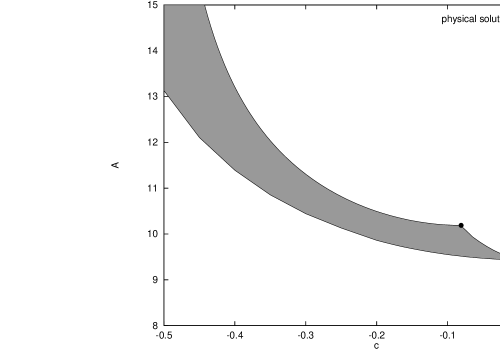
Figure 3: double-cut solutions

The constraint $u(h)\leq 1$ must be satisfied for all $h$ in order for the solution $u(h)$ to correspond to a Young diagram at large $N$. This condition can be used to describe analytically the remaining boundary curves of the physically acceptable region in Figure 3. As one varies $a,b,c,d$ in such a way as to satisfy (5.7), (5.8), and (5.9), the solution (5.5) first fails this condition at the points $b$ and $c$. Thus, we can find the boundaries of the double-cut problem simply by studying the slope of the solution $u(h)$ at the points $b$ and $c$. The boundary of the double-cut solutions arising from the condition that $u(b+)\leq 1$ is

$$(a-b)(K(q)-F(\nu,q))=(a-c)(E(q)-E(\nu,q)).$$ (5.10)

This is the boundary curve at the bottom of the physical region. An analysis of the slope of the solution $u(h)$ near the point $c$, (i.e., requiring $u(c-)\leq 1$) yields an equation for the final boundary of the double-cut region. It reads

$$\rho(b-c)\sqrt{\frac{(1/2-d)(1/2-a)}{(1/2-c)(1/2-b)}}=(a-c)(c-d)(K(q)-F(\nu,q))-\rho^{2}(E(q)-E(\nu,q)).$$ (5.11)

One finds that the solutions at these boundaries are indeed legal solutions, so the double-cut region is closed. It is easy to verify that the $u(c-)\leq 1$ boundary runs precisely between the $A_{+}$ and $A_{-}$.

Having found these new saddle points of the action (2.10) we now study their contribution to the partition function. To begin with, we can see from Figure 3 that for all $A>A_{-}$ there is indeed a one parameter family of solutions to the saddle point equation. However, not all these solutions are actually saddle points, since the saddle point equation is only satisfied in the interior of the regions $(d,c)$ and $(b,a)$. To determine which of the values is the physical saddle point for any given $A$ it would be necessary to compute the exact free energy $F$ and to maximize this quantity across all solutions corresponding to that fixed value of $A$.

Unfortunately, however, an exact calculation of the free energy is technically difficult. The situation here is analogous to that which arises in the full QCD₂ theory. In that case, it was shown by Minahan and Polychronakos [15] that for every value of $A$ above the critical value $\pi^{2}$ there is a family of solutions to the saddle point equation, parameterized by the parameter $Q$ corresponding to the $U(1)$ charge, which is essentially the first moment of $u(h)$. In that case also, a direct calculation of the free energy is difficult. Symmetry arguments would indicate that the DK solutions with $U(1)$ charge $Q=0$ are the physical saddle points in this theory. The correspondence of the strong coupling expansion of the DK solutions with the QCD₂ string gives further weight to this conclusion; however this result has not been rigorously proven.

In the chiral theory, we no longer have a reflection symmetry to rely on; however, the correspondence of the strong coupling expansion of the single-cut solution with the chiral string theory is a strong indication that the free energy is extremized by the single-cut solutions above $A=A_{+}$. We have numerically integrated the free energy in that region and found that indeed $F$ seems to be maximized on the single-cut solution for any fixed $A>A_{+}$. The behavior of the theory in the intermediate phase, however, presents a much more subtle problem. Numerically integrating $F$ indicates that the physical solutions in the intermediate phase lie near or on the boundary (5.11). The numerical analysis of $F$ in this region is extremely delicate, presumably due to the existence of phase transitions at $A_{-},A_{+}$.

Thus, although we have fairly solid evidence that the single-cut solution describes the physical saddle point above $A_{+}$, we are unable to give an exact formula for the curve corresponding to the physical solutions connecting the two critical points. Nonetheless, we can compute the derivative of the free energy along the physical curve using the same method as was used in Section 3 to calculate $F^{\prime}(A)$ in the single-cut region. From the fact that the physical saddle point obeys the classical equations of motion, we find that the derivative of the free energy is related to the second moment of the density function $u(h)$ by

$$F^{\prime}(A)=-\frac{1}{2}\int{\rm d}h\;u(h)h^{2}+1/24.$$ (5.12)

After some algebra one ascertains that

$$\int{\rm d}h\;u(h)h^{2}$$ (5.13)

$$= \big{(}\frac{(1/2-b)(1+W)}{6}+M\big{)}\sqrt{\frac{(1/2-a)(1/2-c)(1/2-d)}{1/2-b}}+M\rho(E(q)-E(\nu,q))$$

$$+(3W^{2}X^{2}+6WXYZ+Y^{2}Z^{2}+2X^{2}Y^{2}+2X^{2}Z^{2}+X^{4})\frac{(K(q)-F(\nu,q))}{192\rho}$$

where

$$W=a+b+c+d\;\;\;\;\;X=a-b-c+d\;\;\;\;\;Y=a+b-c-d\;\;\;\;\;\;Z=a-b+c-d$$ (5.14)

and where

$$M=(3W^{2}+X^{2}+Y^{2}+Z^{2})/48$$ (5.15)

Using the constraint equations (5.7, 5.8, 5.9) allows us to write this expression in terms of algebraic functions of the area $A$ and the points $a,b,c,d$,

$$\int{\rm d}hu(h)h^{2} = \frac{(1/2-b)(1+W)}{6}\sqrt{\frac{(1/2-a)(1/2-c)(1/2-d)}{1/2-b}}+M$$ (5.16)

$$+(6WXZY+Y^{2}Z^{2}+X^{2}Y^{2}+X^{2}Z^{2})A/768$$

As a simple check note that in the limit $b\rightarrow a$ this expression leads to the result of (3.22). We have thus given an explicit formula for the derivative of the free energy in the double-cut region which is applicable to whatever curve describes the physical solutions in that region, although we have been unable to describe the curve analytically. If one could derive an analytic formula for the physical solutions in the intermediate region, (5.16) could be used to calculate the order of the phase transition at the two critical points.

6 Conclusions

We have developed a matrix model that describes a single chiral sector of the QCD₂ string. The analysis indicates that there are three distinct regimes for solutions of the saddle point equation of the chiral theory on the sphere. We have shown that there exists a simple single-cut solution which exists for large and small areas and which agrees with the string picture in an expansion around large area. However, this single-cut solution ends (stops leading to physically viable solutions) as one decreases the area from infinity and also as one increases the area from zero. Thus the single-cut solution cannot describe the system for areas $A_{-}<A<A_{+}$. We have shown that for these intermediate areas a saddle point may be found as a double-cut solution to the (integral) equation of motion. This double-cut solution limits to the single-cut solution in the large area regime and connects the upper and lower branches of the single-cut solution. For any fixed $A>A_{-}$ there is a one-parameter continuum of saddle point solutions. When $A>A_{+}$, we have fairly conclusive evidence that the single-cut solution dominates the theory. However, in the intermediate regime we cannot calculate exactly where the curve describing the physical saddle point lies. In fact, although we believe there is only a single curve with maximum free energy connecting the two points $A_{+}$ and $A_{-}$, it is conceivable that there may be multiple physical saddle points in this intermediate region, although numerical evidence indicates that there is indeed only a single such curve, which lies near or on the $u(c-)\leq 1$ boundary (5.11).

Despite our uncertainty regarding the exact location of the intermediate saddle point curve, our analysis gives a fairly complete picture of the theory at any $A$. The dominant stationary solutions are the single-cut solutions for $A\geq A_{+}$ and $A\leq A_{-}$ and there are likely to be a simple trajectory of solutions in the double-cut region that interpolate between these single-cut solutions. The fact that the physical curve of solutions in $(c,A)$ space, as well as the solutions $u(h)$, undergo discontinuities at the points $A_{+}$ and $A_{-}$ indicates that there are probably phase transitions at these points. The behavior of the density function $u(h)$ at the point $A_{-}$ is closely analogous to that of the full QCD₂ density function at the DK phase transition point, suggesting that the chiral theory probably has a third order phase transition at this point. However, an exact characterization of phase transitions in the chiral theory will not be possible until a method is found for determining which of the solutions in the double-cut region actually dominate the partition sum. If this could be accomplished, it would then be straightforward in principle to compute the order of the phase transition at the critical points simply by comparing power series expansions of the free energy $F(A)$ on either side of the critical points.

The single-cut solution of the matrix model gave us an exact analytic formula for the large area regime of the chiral theory. Because this exact formula has a series expansion which is equal to the leading ($N^{2}$) term in the free energy of the chiral string theory, we were able to relate the terms in this expansion to sums over maps between Riemann surfaces. In particular, a calculation of the leading terms in the area polynomials of the expansion allowed us to derive a previously conjectured result on the number of sphere to sphere maps. An interesting direction for further work might be to find further structure in the analytic equations for the large area chiral theory and to relate this structure to the geometry of string maps.

It is remarkable that the location of the critical point bounding the large area phase is relatively insensitive to the details of the theory in question. The result proven here for the number of sphere to sphere maps was used in [11] to show that in a chiral theory with branch points, but without $\Omega$-points, the critical point occurs near $A=11.9$. In this paper we found that the $\Omega$-points in the chiral theory shift the critical point to near $A=10.2$, which is extremely close to the DK critical point in the coupled theory at $A=\pi^{2}\approx 9.9$.

One particularly surprising feature of the results given here is the fact that although the chiral theory apparently has three distinct phases, the large and small area phases are in fact described by the same analytic expressions, indicating some type of duality between these two phases. This situation also bears an striking similarity to the results of [11] where the convergence properties of the string expansion were studied for both the chiral and coupled QCD₂ theories. In that analysis, it was shown that the string expansion of the chiral theory has a radius of convergence approximately equal to the point $A_{+}$, but that the string series also converges for very small areas. A numerical comparison, however, shows that the results of the matrix model disagree with the explicit string sum for small area. The small area phase we have described in this work of course lies outside the radius of convergence of the large area phase. Thus, the fact that the string sum did converge for small $A$ seems mysterious.

In order to further understand the chiral QCD₂ matrix model we have described here, it would be interesting to study directly the free energy of this model. A way of analytically describing the dominant saddle points for $A_{-}<A<A_{+}$ in this model would be invaluable for the computation of the order of the phase transition across the critical loci. Furthermore, an understanding of how to compute $F$ directly might shed some light on the significance of the one-parameter families of solutions described in [15] for the full QCD₂ large $N$ theory.

Acknowledgements

We thankfully acknowledge helpful conversations with S. Axelrod, M. Douglas, D. Gross, J. Minahan, A. Polychronakos, H. J. Schnitzer and I. M. Singer. W. T. would also like to thank the Aspen Center for Physics where part of this work was completed.

References

- [1] A. Migdal, Zh. Eksp. Teor. Fiz. 69, 810 (1975) (Sov. Phys. JETP. 42 413).
- [2] B. Rusakov, Mod. Phys. Lett. A5, 693 (1990).
- [3] E. Witten, Comm. Math. Phys. 141,153 (1991).
- [4] D. Gross, Nucl. Phys. B400, 161 (1993).
- [5] J. Minahan, Phys. Rev. D47, 3430 (1993).
- [6] D. Gross, W. Taylor, Nucl. Phys. B400, 181 (1993).
- [7] D. Gross, W. Taylor, Nucl. Phys. B403, 395 (1993).
- [8] S. G. Naculich, H. A. Riggs, H. J. Schnitzer Mod. Phys. Lett. A8, 2223 (1993).
- [9] M. Douglas, V. Kazakov, Phys. Lett. B319, 219 (1993).
- [10] D. J. Gross, A. Matytsin, Instanton Induced Large Phase Transitions in Two- and Four- Dimensional QCD, preprint PUPT-1459, hep-th/9404004, April 1994.
- [11] W. Taylor, Counting Strings and Phase Transitions in 2D QCD, preprint MIT-CTP-2297, hep-th/9404175, April 1994.
- [12] S. Cordes, G. Moore, and S. Ramgoolam, Large 2D Yang-Mills Theory and Topological String Theory, preprint YCTP-P23-93, hep-th/9402107, February 1994.
- [13] P. Horava, Topological Strings and QCD in Two Dimensions, preprint EFI-93-66, hep-th/9311156, November 1993.
- [14] B. Rusakov, Phys. Lett. B303, 95 (1993).
- [15] J. A. Minahan, A. P. Polychronakos, Nucl. Phys. B422 (1994) 172.
- [16] A. Cayley, Quart. Jnl. Pure Appl. Math 23, 376-378 (1889).
- [17] A. C. Pipkin, “A Course on Integral Equations,” Berlin, Springer, 1991.
- [18] P. F. Byrd, M.D. Friedman, “Handbook of Elliptic Integrals for Engineers and Physicists,” Berlin, Springer, 1954.