SLAC–PUB–6506 May 1994 hep–th/9407039 T Towards Quantum Cosmology without Singularities††thanks: Work supported by the Department of Energy, contract DE–AC03–76SF00515.
Abstract
In this paper we investigate the vanishing of cosmological singularities by quantization. Starting from a 5d Kaluza–Klein approach we quantize, as a first step, the non–spherical metric part and the dilaton field. These fields which are classically singular become smooth after quantization. In addition, we argue that the incorporation of non perturbative quantum corrections form a dilaton potential. Technically, the procedure corresponds to the quantization of 2d dilaton gravity and we discuss several models. From the 4d point of view this procedure is a semiclassical approach where only the dilaton and moduli matter fields are quantized.
We consider a cosmological string solution which has classical singularities (big bang). Near these singularities the theory factorizes in a smooth spherical part and a singular 2d part. This singular part is the well-known dilaton gravity (see e.g. [1]-[4]) and as a first step we are going to quantize this part with the result that all singularities disappear. This procedure is also known as s-wave reduction and was so far used for 4d BH physics.
1. Classical theory. Our 4d classical model is given by
| (1) |
where is a dilaton field, is the torsion corresponding to the antisymmetric tensor field and is a modulus field. A cosmological solution to this model is given by [5]
| (2) |
After a time reparameterization one obtains the standard Friedmann–Robertson–Walker (FRW) metric with as 3d volume form corresponding to the spatial curvature (). The parameter is the minimal extension and for the parameter denotes the maximal extension of the universe. This is obvious after transforming the solution to the conformal time
| (3) |
for which the metric is
| (4) |
|
|
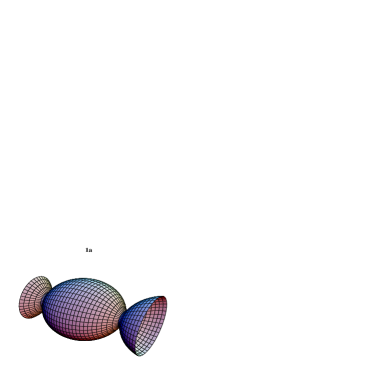
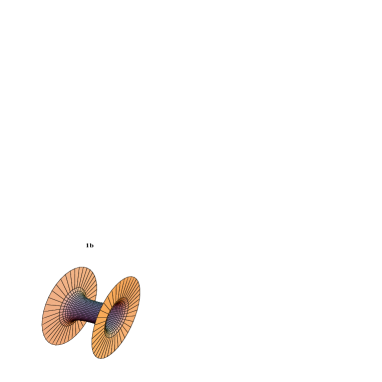
Unfortunately, in [5] no analytic results for the world radius in the standard parameterization of the FRW metric could be found. We have plotted numerical results in figure 1. Figure 1a shows the oscillating solution for and 1b the wormhole solution for . For the solution has again the geometry of figure 1b but with the difference that there are no asymptotic flat regions as for . Remarkably, the scalar fields and have divergencies although the metric behaves completely smooth for all times. To understand this phenomena one has to go back to the 5 dimensional (5d) origin. In the sense of a Kaluza–Klein approach solution (2) can be obtained by dimensional reduction of a 5d theory. Then, the modulus field corresponds to a time dependent compactification radius of the fifth coordinate. The corresponding action is given by the effective string action
| (5) |
and the 5 dimensional solution can be written as
| (6) |
The 5d dilaton is related to by and . For and after switching the signature of the metric ( and ) this 5d solution is just the 5d BH solution (in the conformal time ) discussed by Horowitz and Strominger in [6]. Here, define the two horizons of the theory and our cosmological solution lives between these horizons.
2. S-wave reduction. We are particularly interested in the fate of the singularities if one starts to quantize the theory. Therefore, it is reasonable to restrict ourselves to the region near the singularities (). In this region one can assume that quantum corrections become important. Furthermore, as one can see from (6) in this limit the 5d solution decouples in a 3d spherical part () and a 2d part which is the known dual 2d BH [7]. In the figure it is just the region of minimal extension, e.g. inside the wormhole of fig. 1b.
Before we can start to quantize the 2d part we have to reduce the 5d action (5) down to a 2d theory. Motivated is this procedure by the assumption that the quantum corrections respect the spherical symmetry. Generally, this is not the case but sufficient for a first approximation. In BH physics this procedure is also known as s–wave reduction. For the 5d metric we make the ansatz
| (7) |
where is the 2d metric part. In what follows we quantize only and the dilaton (resp. , see below). The remaining fields are assumed to be classical backgrounds given by (2) or (6). After integrating out the angular degrees of freedom and using the field from (2) we obtain for (5)
| (8) |
with and . Near the singularity () the background field is smooth, (see (6) and (7)) and up to the second order in we can approximate the terms by a constant
| (9) |
with . A classical solution in conformal coordinates is given by [7]
| (10) |
where is constant. This solution can be transformed to the 2d () part of (6) where corresponds to .
3. Quantization. The quantization of (9) has been studied in various papers [1]-[4], [8, 9]. Each of these models will be discussed, but before we do so in detail let us come back to the classical solution once more. The fact that (6) or (2) are independent of tha fifth coordinate leads to the dual solution
| (11) |
Both solutions have a significant difference. Singular points of (6) are regular in (11) and vice versa. Furthermore, in the region that we are interested in () the solution (6) is in the strong coupling region () whereas the dual solution (11) is in the weak coupling region (; if we assume that which is reasonable, since corresponds to the maximal/minimal extension of the universe) Again the 2d part decouples and can be transformed into (10) where corresponds to .
When quantizating this theory we are especially interested in what happens in the strong coupling region, i.e. the fate of the singularity in (6). As a consistency condition of this procedure we have to ensure that in the classical limit (weak coupling region) we get back our classical result (11) which is non singular for . We are following the procedure of de Alwis [8] and later on we discuss the modification concerning the other models. After choosing the conformal gauge
| (12) |
we can rewrite (9) as a general 2d model
| (13) |
with: . Thus, the quantization of the dilaton gravity is reduced to the quantization of a 2d model with the target space spanned by and . This model, however, is well defined only if the background fields and define a 2d conformal field theory. This symmetry is a consequence of the fact, that the original theory depends only on and not on , and thus, has to respect the symmetry: and (see (12)). We transform the theory to an exact model and define the quantum theory by this (exact) conformal field theory (see e.g. [8, 9]). Following this approach we first note that the target space metric has the general structure
| (14) |
where and are model dependent functions of or . For we have the CGHS model [1]; for the model from Strominger [3]; and describes the RST model [4]. The parameter originates from the definition of the functional integration measure and corresponds to additional conformal matter. As next step we introduce new target space coordinates
| (15) |
and obtain a flat metric
| (16) |
(for negative we have to perform a Wick rotation in and ). For this flat metric it is easy to find the dilaton and tachyon that define a conformal field theory. The general solution of the corresponding equations is
| (17) |
The demand to get the classical model (9) in the weak coupling limit yields a further restriction to and . Following the suggestion of de Alwis we set: and and get the known Liouville theory ( as Liouville field) that couples to the matter field
| (18) |
This describes a well defined 2d gravity theory on the classical as well as on the quantum level. The strategy is to define the quantum theory in terms of this action and to regard (9) as the classical limit.
As second step we have to find solutions of the equations of motion for and ()
| (19) |
Solving these equations we have to restrict ourselves to solutions that reproduce the BH solution (10) in the classical limit. Therefore, we are interested in a solution depending on only and find
| (20) |
(). Using the transformation (15) we can express this solution in and . In doing so we have to fix the up to now arbitrary functions and . Let us start with parameterization suggested by de Alwis: , . Motivated is this choice by the fact that for all values of and the transformation (15) is non singular and secondly that the range of and goes from to if and do so. For and one gets
| (21) |
In terms of (20) one finds in the weak coupling limit () the desired classical solution (10)
| (22) |
Since we are in the weak coupling region this solution corresponds to our dual solution (11) which is non-singular for . In the strong coupling limit () we obtain
| (23) |
Therefore, after incorporation of quantum corrections () the black hole solution gets smooth also in the strong coupling region. Note, that in dilaton gravity a singularity in the metric has to be accompanied by a singularity in the dilaton, i.e. singularities can only appear in the strong or weak coupling region. For the other models the picture is qualitatively the same. In the CGHS model () one obtains for (15)
| (24) |
and in strong coupling region this model gives
| (25) |
For the Strominger model () we find ( )
| (26) |
which gives in the strong coupling region
| (27) |
And finally in the RST model (, ) the general solution is given by
| (28) |
In the strong coupling region this model behaves like
| (29) |
Therefore we find that all models have no singularities in the strong coupling region and yield the classical result in the weak coupling region.
One can now ask what is the influence of this quantization procedure for the further evolution of the universe. For the derivation of our results it was crucial that the solution decouples in a 2d (dilaton gravity) part and a 3d spherical part. This is valid only if one considers the theory, e.g. ,inside the wormhole of fig. 1b. Extending this procedure to the region away from the wormhole seems to be difficult. But nevertheless, quantum correction inside the wormhole can form a dilaton potential which could be a source of an inflationary period in later times. A dilaton potential in our original action (1) or (5) corresponds to an additional tachyon contribution in the 2d action which is independent of (since was correlated to the constant field in the wormhole, see (8)). The tachyon we have discussed so far is only one possibility. This solution has the advantage that the renormalization group functions vanish thereby yielding a finite 2d quantum field theory. The most general tachyon field, however, is a combination of contributions given by (17). A further additive tachyon term is given by (for )
| (30) |
where the function is given by (15) This term, discussed e.g. in [8] and [10], has in the weak coupling region for all discussed models the typical non-perturbative structure
| (31) |
where is the string coupling constant. Therefore this term vanishes very rapidly in the weak coupling (classical) region and becomes important in the strong coupling region. Furthermore, since is a function of the dilaton only, this tachyon term represents a candidate for a dilaton potential created by non-perturbative quantum corrections in the strong coupling region. If we insert the values for the several models (21), (24), (26) and (28) we obtain different potentials. But all these potentials have no local or global minima and are probably not good candidates to discuss an inflationary period (see e.g. [11] and refs. therein). It remains an open question whether another choice of the model dependent functions and could yield a more appropriate potential.
4. Discussion. Starting with a classical solution of the low energy string effective action we investigated the quantization near the cosmological singularity. Via a 5d Kaluza–Klein approach this solution was obtained as a dimensional reduced theory. Near the singularity the 5d theory decouples in a 3d non singular (spherical) part and a singular 2d part. As a first step we have quantized only this singular 2d part (s-wave reduction). The results (21) - (29) show that for all models the singularity disappears after the quantization of the theory, i.e. the 2d metric part and the dilaton remains finite. An interpretation of this result is that the wormhole becomes traversable via quantum corrections. In addition, we have shown that the incorporation of non perturbative quantum corrections form a dilaton potential. The discussion of the possible structures of the potential created by this procedure remains an interesting task for further investigations.
We used the 5d theory to get contact with the known dilaton gravity. But it is also possible to quantize the 4d theory (1) directly. Our approximation to quantize only the divergent 2d part in 5 dimensions is effectively the same as to quantize the dilaton and moduli matter fields only. Note that the 2d metric part has only one degree of freedom. In the conformal gauge (12) this is the Liouville field but we can also take another gauge, e.g. and then is our moduli field (see (6)). Thus, from the 4d point of view we replaced the dilaton and moduli contributions in the Einstein equation by its vacuum expectation value
| (32) |
where is the metric in the Einstein frame. Classically, the 4d string metric was smooth but the Einstein metric was singular (caused by the dilaton and moduli). However, after quantization the singularities in the scalar fields disappeared and thereby also the Einstein metric turned out to be non-singular. This implies that similar to the string frame the Einstein metric describes a universe which starts and ends (for ) not with a singularity but with a minimal (nonzero) extension (wormhole). Therefore, in both frames the spatial part of the universe is qualitatively given in figure 1. Of course, the quantization of the scalar fields near the singularity can only be a first step and future investigations have to show whether a complete quantum theory will leave this qualitative feature intact.
Acknowledgments
We would like to thank S. Förste and J. García-Bellido for
useful comments. The work of K.B. is supported by a DAAD grant and of
T.T.B. by the Swiss National Science Foundation. The work of both
authors was also supported by the US Department of Energy, contract
DE-AC03-76SF00515.
References
- [1] C.G. Callan, S.B. Giddings, J.A. Harvey, A. Strominger: “Evanescent black holes”, Phys. Rev. D45 (1992) 1005;
- [2] T.T. Burwick, A.H. Chamseddine: “Classical and quantum consideration of 2d gravity”, Nucl. Phys. B384 (1992) 411;
- [3] A. Strominger: “Faddeev–Popov ghosts and (1+1) dimensional black hole evaporation”, Phys. Rev. D46 (1992) 4396;
- [4] J.G. Russo, L. Susskind, L. Thorlacius: “End point of Hawking radiation, Phys. Rev. D46 (1992) 3444;
- [5] K. Behrndt, S. Förste: “String–Kaluza–Klein cosmology”, preprint SLAC–PUB–6471, RI–2–94 (hep-th: 9403179); K. Behrndt, S. Förste: “Cosmological string solutions in 4 dimensions from 5d black holes”, Phys. Lett. B320 (1994) 253;
- [6] G.T. Horowitz, A. Strominger: “Black strings and p-branes”, Nucl. Phys. B360 (1991) 197;
-
[7]
E. Witten: “String theory and black holes”, Phys. Rev. D44 (1991) 314;
A. Giveon: “Target space duality and stringy black holes”, Mod. Phys. Lett. A6 (1991) 2843; - [8] S.P. de Alwis: “Quantum black holes in two dimensions”, Phys. Rev. D46 (1992) 5429;
- [9] A. Bilal, C. Callan: “Liouville model of black hole evaporation”, Nucl. Phys. B394 (1993) 73;
- [10] J.G. Russo, A.A. Tseytlin: “Scalar–tensor quantum gravity in two dimensions”, Nucl. Phys. B382 (1992) 259;
- [11] R. Brustein: “The role of the superstring dilaton in cosmology and particle physics”, preprint CERN–TH.7255/94 (hep–th/9405066).