Replica Field Theory for Deterministic Models: Binary Sequences with Low Autocorrelation

Abstract

We study systems without quenched disorder with a complex landscape, and we use replica symmetry theory to describe them. We discuss the Golay-Bernasconi-Derrida approximation of the low autocorrelation model, and we reconstruct it by using replica calculations. Then we consider the full model, its low $T$ properties (with the help of number theory) and a Hartree-Fock resummation of the high-temperature series. We show that replica theory allows to solve the model in the high $T$ phase. Our solution is based on one-link integral techniques, and is based on substituting a Fourier transform with a generic unitary transformation. We discuss this approach as a powerful tool to describe systems with a complex landscape in the absence of quenched disorder.

hep-th/9405148
ROM2F/94/015
Roma-La Sapienza 1019

1 Introduction

This note has been prompted by two main motivations. One comes from a problem whose solution has relevant practical applications, while the other one is more abstract in nature, and is generated from what we have learned in the last years about disordered systems [1, 2].

We will be dealing with the problem of finding binary sequence with low autocorrelation [3, 4, 5]. Sequences of this kind are important in favoring efficient communication, and the practical side of the problem is obvious. We hope we will convince the reader it is also fascinating from a theoretic point of view.

When we search binary sequences of $+1$ and $-1$ having minimal autocorrelation we are dealing with a completely deterministic problem, and disorder is not a part of the game. In our starting rules there is nothing random. Still, we will see how the system can indeed have a behavior that is very much reminiscent of a random system. Changing one spin to optimize a given set of correlations can increase other correlation functions, with a competitive effect which turns out to be typical of a system which contains disordered couplings. We will see that replica symmetry theory [1, 2] can be an useful tool even for describing this kind of systems. We will be able, by using the analogy with a relevant disordered system, to capture the general features of the model. We will try to understand and stress the differences which distinguish a low autocorrelation model from a spin glass like model. That will lead us to a detailed discussion of the low temperature properties of the low autocorrelation model.

We present a careful investigation of some statistical mechanics aspects of the problem, by largely extending previous results due to Golay [4] and to Bernasconi [5]. We establish a relation between this deterministic problem and random spin glasses, which we consider a very interesting outcome of this study. Some ideas typical of spin glasses, as replica symmetry breaking, can be successfully used in this context.

In section (2) we define the models we will discuss in the rest of the paper. In section (3) we discuss the ground state structure of the model (also by using well known number theory, see for example [6]) and we begin a discussion of its phase diagram and of the low temperature phase. In section (4) we discuss the validity of the Golay-Bernasconi approximation. We introduce the replica symmetry approach, we define a disordered model and we study its behavior. In section (5) we investigate in better detail the high-temperature regime. We perform and describe a high-temperature expansion. We introduce a Hartree-Fock approximation which allows us to write a closed form for the free energy.

In section (7) we discuss the full phase diagram of the model. In section (6) we introduce one more model which can be solved by using the replica approach. The solution is the same we get with the Hartree-Fock approximation. In section (8) we draw our conclusions.

The reader which will find this problem interesting will be happy to know that much related material is becoming available. Reference [7] mainly contains a study of the dynamical properties of the system, which uses the tempering Monte Carlo approach [8]. Ref. [9] discusses aging in low autocorrelation models. Reference [10, 11] introduces and discusses more models and analogies with random systems (and, in particular, the open low autocorrelation model, see later). More results, which partially overlap with ours, will be discussed by Bouchaud and Mezard in [12].

2 Definition of the Model

Let us consider a sequence of length $N$ of spin variables $\sigma_{j}$. They are labeled by a one-dimensional index $j$ ($\sigma_{j}$, $j=1,N$), and can take the values $\pm 1$. The Hamiltonian is defined by

$$H\equiv\frac{1}{N-1}\sum_{k=1}^{N-1}C^{2}_{k}\ ,$$ (1)

where $C_{k}$ is the sum of the $\sigma_{i}-\sigma_{j}$ correlation functions at distance $k\equiv|i-j|$. The choice of the boundary conditions, i.e. of the terms we will include in the sum (1), allows us to define two different models.

• The open model is defined by using open boundary conditions. In this case $C_{k}$ is obtained by summing $N-k$ terms:

  $$C_{k}\equiv\sum_{j=1}^{N-k}\sigma_{j}\sigma_{j+k}\ .$$ (2)

• The periodic model is defined by using periodic boundary conditions. Here we are considering a closed chain, and:

  $$C_{k}\equiv\sum_{j=1}^{N}\sigma_{j}\sigma_{(j+k-1)(\mbox{\footnotesize mod}N)+1}\ .$$ (3)

  Here we have summed $N$ contributions, considering all spin couples at distance $k$ on the closed chain.

The periodic model has some peculiarities which allow us to study it in greater detail. The main tool we will use is the Fourier transform. We can rewrite the periodic Hamiltonian as

$$H={1\over N-1}\sum_{p=1}^{N}(|B(p)|^{4}-1)+1\ ,$$ (4)

where the $B(p)$ are the Fourier transformed $\sigma_{i}$, and the Fourier transform is defined as

$$B(p)\equiv\frac{1}{\sqrt{N}}\sum_{j=1}^{N}e^{i\frac{2\pi p}{N}j}\sigma_{j}\ .$$ (5)

In eq. (4) we had to subtract a constant factor since in the sum of eq. (1) we do not include the constant correlation at distance zero.

In this paper we will focus on the periodic model. Further results about the open model will be contained in ref. [11].

As we have already discussed much attention has been devoted in the past to the problem of finding the ground state of such a model [3, 4, 5]. Here we will continue such an effort, but we will also (and mainly) extend our study to the thermo-dynamical behavior of the model. We will study its behavior as a function of the inverse temperature $\beta\equiv\frac{1}{T}$. Our main efforts will be devoted to the computation of free energy density. We define the partition function of our system as

$$Z_{N}(\beta)\equiv\sum_{\{\sigma\}}e^{-\beta H(\{\sigma\})}\ ,$$ (6)

where the sum runs over the $2^{N}$ allowed configurations of the spin variables, and the free energy density as

$$f(\beta)\equiv\lim_{N\to\infty}\ (-{1\over\beta N}\ \ln(Z_{N}(\beta)))\ .$$ (7)

Once again, we note that this approach has both a practical interest and a theoretical one. It is interesting to study the full thermo-dynamical behavior of the system since that gives more information about features of the low autocorrelation sequences. We will be interested for example in their number and their basin of attraction, and in their stability properties (which can be very relevant for practical applications). On the other side such a statistical mechanics approach will help us to shift towards the realm of disordered systems.

3 The Ground State Energy and a First Look at Thermodynamics

The ground state of the periodic model defined by the Hamiltonian (1) (with $C_{k}$ given by (3)) is not known in general. No systematic procedure to construct ground state configurations for generic $N$ is known. A remarkable exception holds for given values of $N$, where ad hoc constructions exist. Such constructions are mainly based on number theory [6], and they produce spin sequences with a total energy of order $1$, i.e. with an energy density $e\equiv\frac{H}{N}$ of order $\frac{1}{N}$ (which tends to zero in the thermo-dynamical limit).

Let us describe a simple construction, which works when $N$ is a prime larger than $2$ [6]. We set the $\sigma_{j}$ variables to $-1$, $0$ or $+1$ by identifying

$$\sigma_{j}=j^{{1\over 2}(N-1)}\mbox{\rm mod }N\ .$$ (8)

In this way we get $\sigma_{j}=\pm 1$ for $j<N$, and $\sigma_{N}=0$. For example for $N=13$ by using this construction we get the sequence

$$\begin{array}[]{cccccccccccccc}j&1&2&3&4&5&6&7&8&9&10&11&12&13\\ \sigma_{j}&+1&-1&+1&+1&-1&-1&-1&-1&+1&+1&-1&+1&0\end{array}$$

By following this procedure we have obtained a sequence which, but for its last spin, is a legitimate one (in the sense it is composed by $\pm 1$). Now we will proceed by first evaluating the energy of this quasi-legal sequence, and eventually by computing the effect of modifying the last spin to $\pm 1$, to get a truly legal sequence. We will show that such a sequence is in some cases a true ground state (i.e. it has the minimum allowed energy).

Computing the energy of such a sequence is an easy task. Theorems well known by mathematicians [6] tell us that in this case all correlation functions $C_{k}$ are equal to $-1$ (we remind the reader we are discussing the periodic model). We can also use a Gauss theorem [6] to notice that the Fourier transformed variables take here the form

$$B(p)=G(N)\ \sigma_{p}\ ,$$ (9)

where $G(N)=1$ if the prime $N$ has the form $4n+1$ (with positive integer $n$), and $G(N)=-i$ if it has the form $4n+3$ (in different words on our sequences the Fourier transformed variables are equal or proportional to the original $x$-space variables). It is clear that the Hamiltonian (1) of the periodic model takes on our slightly-illegal spin sequence the value $1$.

Now we have to understand what happens when we modify the spin $\sigma_{N}$, by setting it to $\pm 1$. It is easy to see that when we do that the Hamiltonian changes of a finite amount. Indeed for $N$ of the form $4n+3$ the Hamiltonian does not change, and keeps it value of $1$. The point is that (as can be easily verified by inspection) the $\pm 1$ sequences are in this case antisymmetric around the site $N$. For $N$ of the form $4n+1$ the $\pm 1$ sequences are symmetric around the site $N$, and on the fully-legal sequence $H$ takes a value of $5$.

Since we are considering $N$ odd, it is clear that for $N$ prime of the form $4n+3$ the two fully legal sequences we have built (and the sequences obtained by using the translational invariance of the problem, and the $\pm 1$ symmetry) are true ground states. This is because for $N$ odd the minimum value allowed for each $C_{k}$ is $1$, and the minimum value allowed for $H$ is $1$. We have exhibited configurations with the minimal allowed energy, i.e. ground states.

Let us state again our conclusion. In the case of $N$ prime of the form $4n+3$ we have obtained a thermodynamical ground state, whose energy density goes to zero when the volume goes to infinity. Translational invariance and spin flip invariance imply that the degeneracy of the ground state is at least $2N$.

For other values of $N$, for example of the form $N=2^{p}-1$, there are alternative techniques to construct the ground state, based for example on the theory of Galois fields [6]. For example for $N=2^{57}-1=144115188075855871$ one finds that the sequence which satisfies the relation

$$\sigma_{j}=\sigma_{j-24}\sigma_{j-57}$$ (10)

is a ground state. If we exclude the trivial case of $\sigma_{i}$ identically equal to $1$ (which is not a ground state), such sequence is unique, apart from a translation [6, 13].

It is rather interesting to note that also in this case the Fourier transform is very similar to the original sequence. One finds that it exists a value of $s$ such that

$$B(p)=\sigma_{p+s}\ .$$ (11)

The deep reasons for this duality among configuration and Fourier space escape us.

It is quite remarkable that this last sequence is considered at all practical effects a good random sequence (see for example [13]). We can summarize the status of things by saying that the ground state of our model can be obtained as the output of a random number generator! This is surprising, but maybe not so much. When designing a random number generator one wants bit sequences with low autocorrelation. That means that for large values of $N$ the correlation functions should not be proportional to $N$. A true sequence of random numbers should have autocorrelations of order $N^{\frac{1}{2}}$. One is doing “better” than that by obtaining sequences with autocorrelation of order $1$. That does not seem to cause any practical problem.

For generic values of $N$ we do not have any method to explicitly exhibit the ground state, and we do not know the ground state energy. The very existence of the thermodynamic limit is non trivial. One could get different results when $N$ goes to infinity depending on the arithmetic properties of $N$ sequence one selects. We shall see later that in the high-temperature region the $N^{-1}$ corrections are different for sequences consisting of even or odd values of $N$. The corrective terms proportional to $N^{-3}$ also change depending if one selects an $N$ series such that $N$ is or not multiple of $3$. We will see that in general things become more and more complex when we look at higher order corrections.

In order to get the first hints about the ground states and the thermodynamical behavior of the system we have used two approaches. In first we have solved exactly (by computing the density of states by exact enumeration) systems of size up to $N=38$. By examining all configurations we have computed the number of configurations of a given energy ${\cal N}(E)$ as a function of $E$. We have looked at the ground state energy $E_{0}$, and stored and analyzed the ground state and the first excited state configurations (at least for some of the $N$ values). From ${\cal N}(E)$ we are able to reconstruct the partition function, the free energy density and all the related thermodynamical quantities.

As a second step we have looked for the ground state energy by using a minimization procedure. For a given $N$ value we start from a random $\sigma_{i}$ configuration, and we minimize its energy by single spin-flips. We repeat this procedure until satisfaction. We assume we have reached the ground state when the minimum energy has been found $F$ times. In the case where we also have the exact solution ($N\leq 38$) this procedure easily gives the correct ground state energy. The choice of $F=100$ recognitions is still safe in the $N$ region going up to $N=50$. Low energy states with a small basin of attraction are the most dangerous. For the case of the good prime $N=47$ (where by good we mean here of the form $4n+3$) the first excited state is found a number of times of order of $50$ before finding the true ground state (which in this case, as we have explained, we know exactly).

In fig. 1 we plot ($N-1$) times the ground state energy as a function of $N$. The small filled triangles are from the minimization search. For $N\leq 38$ they are circled by larger empty dots (that reminds the reader that in this case we also have the exact result, which coincides with the the minimization result).

Figure 1: The ground state energy times $(N-1)$ as a function of $N$. The small filled triangle are from the minimization search. For $N\leq 38$ where we also have the exact solution the small triangles are circled by larger empty dots.

At a first look the ground state energy ($E_{0}$) depends quite randomly on $N$. But we notice some regular patterns which can be of some importance.

• For $N$ prime of the form $4n+3$ the ground state energy is the one given by the exact construction we have described before. This is a test of our programs and procedures.

• For $N$ of the form $4n+2$, $n$ zero and positive integer, i.e. for all the $n$ we have analyzed, we find

  $$E_{N}=4\ .$$ (12)

  We cannot be sure that this behavior is not an accident, but we have to notice we find it for all values of $N$ of this kind.

• For $N$ of the form $4n+1$, $n\geq 8$, i.e. for $N\geq 33$, we have found that

  $$E_{N}=5-\frac{96}{N-1}\ .$$ (13)

  For $N$ of this form, even for $N$ prime, our number theory based ground state construction does not necessarily give a ground state.

We can use these results to try some claims about the $N\to\infty$ limit for the ground state energy. The merit factor, used for estimating how good a low autocorrelation sequence is, for a sequence of length $N$ (and $N$ large, or to agree with standard definitions we need to multiply times $N$ and divide times $N-1$) is given by

$$F^{(N)}\equiv\frac{N}{E^{(N)}}\ .$$ (14)

If the energy goes to a constant value in the large $N$ limit that means that the system will have a zero energy density, and a diverging merit factor. We know that on the primes $N$ of the form $4n+3$ this is exactly what happens. But we also know that such $N$ values have zero measure, and selecting such a sequence could not be a reliable way to go to the infinite volume limit for generic values of $N$. If the behavior we have described in equations (12),(13) survives in the large $N$ limit we have two finite measure sequences (including one $N$ value over $2$) which have asymptotically a zero energy density. On the other $N$ values we are not able to draw even tentative and qualitative conclusions like the above.

The number of configurations of a given energy ${\cal N}(E)$ allows us, as we have explained, to evaluate the thermodynamical properties of the system. In figures (2a-d) we show ${\cal N}(E)$, the number of configuration of energy $E$ as a function of $E$, respectively for $N=31$ (a good prime), $33$ (of the form $4n+1$, non prime), $34$ (of the form $4n+2$) and $37$ (of the form $4n+1$, prime). In figures (3) and (4) we show respectively the internal energy minus the ground state energy (normalized between zero and one) and the specific heat as a function of $T$, for the same $N$ values and a smaller volume, $N=19$.

Figure 2: ${\cal N}(E)$, the number of configuration of energy $E$ as a function of $E$. (a): $N=31$ (a good prime); (b) $N=33$ (of the form $4n+1$, non prime); (c): $N=34$ (of the form $4n+2$); (d): $N=37$ (of the form $4n+1$, prime)

Figure 3: The internal energy $E(T)$ minus the ground state energy (and normalized between zero and one) as a function of $T$, respectively for $N=19$ and $N=31$ (good primes, respectively dots-dashes and dots), $33$ (of the form $4n+1$, non prime, short dashes), $34$ (of the form $4n+2$, long dashes) and $37$ (of the form $4n+1$, prime, continuous line)

Figure 4: As in figure (3), but for the specific heat as a function of $T$.

At this point we are able to draw a few tentative conclusions.

• Changing $N$ of a small amount, typically of a $\Delta N=1$ (when $N$ is already of order $40$), induces large variations in thermodynamic observable quantities in the low $T$ region. Fluctuations from one volume size $N$ to a similar one are large, and macroscopic. Such fluctuations forbid any simple extrapolation to the $N\to\infty$ infinite volume limit. They decrease however for increasing $N$. Their amplitude is compatible with being proportional to $N^{-1}$ also at finite temperature.

• A pronounced peak in the specific heat increases with $N$, strongly suggesting that in the infinite volume limit the system undergoes a phase transition. The $T$ position of the maximum of the specific heat decreases with increasing $N$ (in an irregular pattern). In the region of $N\simeq 30-40$ from the position of the peak we estimate a critical temperature $T_{c}\simeq 0.5$. The nature and the order of the phase transition are difficult to assess.

• The density of states ${\cal N}(E)$ for low energies depends on $E$ approximately as

  $${\cal N}(E)=2N\ e^{A\ E}$$ (15)

  (remember that the minimal degeneracy of the ground state is $2N$). In our $N$ region $A$ turns out to be strongly dependent on $N$. Such a dependence can be fitted well by a linear behavior. This is the same effect we can see in the $N$ dependence of the location of the peak in fig. (4). For our large $N$ values (of order $30-40$) the constant $A$ is of the order of $1.5$.

• The configurations with energy slightly larger that the ground state energy are in average not similar to the ground state. The typical mutual overlap of a ground state and a first excited state is not large when $N$ increases. In particular typical first excited state configurations are not obtained by a single spin-flip operation on one of the ground states. The configurations which are generated by a single spin-flip on the ground state have in average energy higher than the first excited state. For example in the case of $N$ prime of the form $4n+3$ the energy gap among the ground states and its one spin-flipped excitation is at least of $3$. In this case no first excited state is a single spin-flip of the ground state.

  Let us analyze this point in better detail. For a ground state configuration $s_{0}^{\alpha}$ (the series of the $N$ spin variables $\sigma$ which form the ground state $\alpha$) we define the overlap with the first excited state as

  $$O^{\alpha}_{(0,1)}\equiv\frac{1}{N-2}\max_{A}(s_{0}^{\alpha}\cdot s_{1}^{A})\ ,$$ (16)

  where $A$ runs over all first excited state configurations, $\alpha$ can take values over all ground state configurations, and the $\cdot$ is the sum over sites of the product of the two spin variables. $O^{\alpha}_{(0,1)}$ is $1$ when the ground state $\alpha$ corresponds to a first excited state which differs from the configuration $\alpha$ in a single spin flip. This is the maximum possible overlap. If there is the same number of equal spins and different spins $O^{\alpha}_{(0,1)}=0$. For a given $N$ value we define the maximum overlap of the ground state and the first excited state as

  $$O_{(0,1)}^{M}=\max_{\alpha}O^{\alpha}_{(0,1)}\ ,$$ (17)

  where the maximum is taken over all configurations which have the minimum energy. We plot $O_{(0,1)}^{M}$ as a function of $N$ in fig. (5). The maximum overlap is $1$ only for a few values of $N$ (for large $N$, the ones of the form $4n+2$). For good primes it is always very low.

  

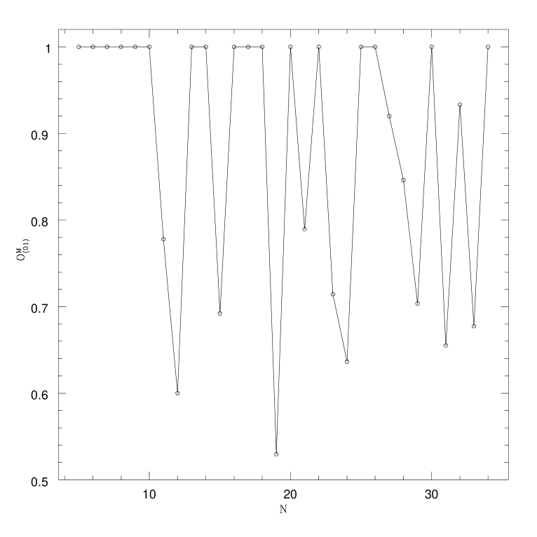
  Figure 5: $O_{(0,1)}^{M}$ as a function of $N$.

  A more useful information can be gathered if we look at the average ground state to first excited state overlap. We define

  $$\langle O_{(0,1)}\rangle\equiv\frac{1}{{\cal N}_{0}}\sum_{\alpha}O^{\alpha}_{(0,1)}\ ,$$ (18)

  where ${\cal N}_{0}$ is the sum runs over all ground states and ${\cal N}_{0}$ is their number. We plot $\langle O_{(0,1)}\rangle$ in fig. (6). As $N$ increases the average overlap decreases, and for $N>22$ we never find a very large average overlap between ground and first excited states.

  

  Figure 6: $\langle O_{(0,1)}\rangle$ as a function of $N$.

  At last we plot in fig. (7) the ground state energies, the first excited state energies and the average energy of configurations obtained by a single spin flip from the ground state (all of them multiplied times $(N-1)$). The difference between single spin flip and first excited state is large, and in this case (even more than in fig. (6)) the effect does not depend dramatically from the cardinality of $N$.

  

  Figure 7: $(N-1)$ times the ground state energy (continuous curve), first excited state energy (dashes) and average energy of configurations obtained by a single spin flip from the ground state (dots) as a function of $N$.

• Few configurations with very small energy start to dominate the partition function at low $T<T_{c}$. We note that our estimate for the constant $A$ coincides with our finite size estimate for the critical temperature (from the location of the specific heat peak). The relation $T_{c}\simeq\frac{1}{A}$ (which holds in the REM model [15]) seems to apply here with reasonable precision.

  This scenario is very similar to the one we are used to see in spin glasses, when a replica symmetry broken phase exists. In particular it reminds of Derrida’s Random Energy Model (REM) [15], where at low temperature only a very small set of configurations dominates the partition function [15, 16].

• As we can already see from fig. (4) the specific heat becomes very small in the low temperature region. Very likely it is exponentially small in the thermodynamical limit. We expect that the $N^{-1}$ corrections (which in the REM [15] are proportional to $(N(\beta-\beta_{c}))^{-1}$) dominate the specific heat in the low temperature phase for $N$ not too large.

• Derrida’s model does not have the divergence of the specific heat at the transition point which we have here. This is likely to be the signature of a transition of a different nature than the one in Derrida’s model.

4 The Golay-Bernasconi Approximation and a First Replica Computation

Let us try now to give an approximate analytic evaluation of the thermodynamical properties of the model. We will follow the approach Golay [4] has originally introduced (see also Bernasconi work [5]) for the open model, and apply it to the periodic model. We will stress the interest and the obvious limitations of such a simple approximation (which basically amounts to consider the correlation functions $C_{k}$ as independent variables).

Let us consider the periodic model, and the correlation function $C_{k}$ as defined from eq. (3). The basic observation is that on a generic random configuration of the $\sigma$ the correlation functions turn out to be also independent variables, randomly distributed according to a Gaussian distribution with variance $N$. Therefore for the probability distribution of the correlation function $C_{k}$ we can write

$$P(C_{k})=(2\pi N)^{-\frac{1}{2}}\ e^{-\frac{C_{k}^{2}}{2N}}\ ,$$ (19)

which holds under our statistical independence hypothesis. Here $k$ can vary from $1$ to $N$. Let us take $N$ odd. Since in this case the correlation functions satisfy the relation

$$C_{k}=C_{N-k}$$ (20)

for all $k$ values, the Hamiltonian (1) can be rewritten as

$$H\equiv{2\over N-1}\sum_{k=1}^{\frac{N-1}{2}}C^{2}_{k}\ .$$ (21)

In this case we only need to consider $\frac{N-1}{2}$ modes. For even $N$ we should add to $H$ the contribution at $k=\frac{N}{2}$ without the factor $2$.

In this approximation the partition function is given by

$$Z(\beta)=2^{N}\prod_{k=1}^{\frac{N-1}{2}}\ \{\ \int dC_{k}\ P(C_{k})\ e^{-\beta H(C_{k})}\ \}\ ,$$ (22)

where we have used (20) and (21) to have $k$ running only up to $\frac{N-1}{2}$. Substituting we get

$$Z(\beta)=2^{N}\prod_{k=1}^{\frac{N-1}{2}}\{\int\frac{dC_{k}}{\sqrt{2\pi N}}\ e^{-C_{k}^{2}(\frac{1}{2N}+\frac{2\beta}{N-1})}\}\ .$$ (23)

For $N$ large we finally get

$$Z(\beta)=e^{N\ (\ln(2)-\frac{1}{4}\ln(1+4\beta))}\ .$$ (24)

We have obtained the expression (24) under the assumption that the $\sigma_{i}$ are independent variables (and then also the $C_{k}$ are). This is obviously not true as soon as $\beta>0$, and expression (24) fails. Indeed the $C_{k}$ are not Gaussian independent random variables. For $\beta>0$ when evaluating the partition function we sample the tail of the probability distribution $P(C_{k})$, where the expression (19) is not valid (we will see that the high $T$ expansion does not coincide with the correct one even at first order). Here we are trying to understand (until now lacking a better approach: but see later) if at least in a high-temperature phase eq. (24) can be an useful approximation to the true behavior of our system.

From the approximated result for the partition function of (24) we can compute the free energy density (7), and the usual thermodynamical energy density and entropy. We find

$$f(\beta) = \frac{1}{\beta}(\frac{1}{4}\ln(1+4\beta)-\ln(2))\ ;$$

$$e(\beta) = {1\over 1+4\beta}\ ;$$ (25)

$$s(\beta) = \ln(2)-\frac{1}{4}\ln(1+4\beta)+\frac{\beta}{1+4\beta}\ .$$

The behavior of the energy density is quite reasonable, while the entropy density $s(\beta)$ becomes negative at low temperature (it goes to $-\infty$ at $T=0$). The entropy density $s(\beta)$ becomes zero at $\beta_{G}=10.3702$, where the energy density has the value $e_{G}\equiv e(\beta_{G})=.02354$.

A possible approximated approach to the problem (along the direction hinted by Golay and Bernasconi) would be based on saying that this solution is close to the correct one in the high $T$ phase, for $\beta\leq\beta_{G}$. One would then claim that a good approximation is to state that for $\beta>\beta_{G}$ general thermodynamical properties (i.e. the fact that both the specific heat and the entropy are not allowed to become negative) imply that the energy density has to remain constant

$$e(\beta)=e_{G}\ ,\ \ \forall\ \beta\geq\beta_{G}\ .$$ (26)

We have a scenario which is very reminiscent of the REM [15]. As we have already noticed an obvious drawback of this point of view, which is built on a series of arbitrary assumptions, is that it does not reproduce correctly even the first non-trivial order of the high $T$ series expansion. It captures however some of the relevant features of the model (like for example the presence of an abrupt transition at finite $T$), and it seems worthwhile to try to understand better its features.

Now we will try to apply the replica method to the problem of sequences with low autocorrelation (at a first stage to try to recover the results of the Golay-Bernasconi-Derrida (GBD) approximation we have just discussed). We know that replica methods have been applied with good success [1, 2] to the analysis of systems whose behavior has remarkable similarities to the one of our low autocorrelation sequences. Yet, until now replica approach has been dealing with system in which quenched randomness plays a major role. There is nothing of a priori random in our low autocorrelation sequences, and the replica method could seem here out of place.

However if it is true that the generic properties of the behavior of low autocorrelation sequences have something to do (at least for not too low $T$) with the ones of a system with quenched disorder. Then we can hope to use the replica techniques.

We will want a random system which mimics the properties of our original ordered system. We will have to identify such a system on the basis of some general principle, and we will see that this will be more or less easy in the different cases.

One possible approach is based on considering a Hamiltonian

$$H_{\{J\}}(\{\sigma\})\ ,$$ (27)

which depends on the quenched control parameters $\{J\}$, which are randomly distributed. For a particular realization of the sequence $\{J\}$ such random Hamiltonian coincides with our original Hamiltonian (in the present case with (21)). Let us suppose that we are able to use the replica approach to compute the average of the thermodynamic functions for the system described by (27). Now we can hope that the result obtained for a generic realization of the random variables $\{J\}$ is the same we would have obtained by selecting the exact $\{J\}$ sequence which leads to the original Hamiltonian (21)). In this case the replica symmetry gives the correct result for the deterministic model. This way of reasoning is potentially very dangerous, and can lead to disaster. The $3d$ Edwards-Anderson model, once understood (for recent progresses see [17]), will not very probably lead to the same solution of the ferromagnetic $3d$ Ising Model. The issue here deals with how generic is the special $\{J\}$ sequence which gives the original deterministic Hamiltonian, and cannot be solved a priori. A posteriori for example one can verify if the deterministic and the random models have the same high-temperature expansion (of course this may lead to surprises in the low temperature region).

A second possible approach is based on the introduction of a control parameter $\epsilon$, and of a Hamiltonian

$$H_{\epsilon,\{J\}}(\{\sigma\})\ ,$$ (28)

which interpolates from the random Hamiltonian at $\epsilon=0$ to the deterministic Hamiltonian at $\epsilon=1$. If the interpolation is smooth and there are no phase transitions in the interval $0<\epsilon<1$ the perturbative expansion around the result $\epsilon=0$ (which one should be able to obtain) could be used to estimate the results for $\epsilon=1$.

This is the general framework. We hope that, by using one of these approaches, replica method will enable us to obtain qualitative and quantitative predictions about the deterministic problem.

Let us start by trying to reproduce the GBD result (i.e. the simple approximation we have just studied) in the framework of replica theory. Our aim will be to consider a soluble random model such that the probability distribution of correlation functions is Gaussian, as in (19). In the high-temperature phase the free energy density of such a model should be given by the GBD approximation.

We will consider the Hamiltonian

$$H\equiv{2\over N-1}\sum_{k=1}^{\frac{N-1}{2}}{\tilde{C}}^{2}_{k}\ .$$ (29)

In this new model the ${\tilde{C}}_{k}$ are not simply correlation functions anymore, but they are given by

$${\tilde{C}}_{k}\equiv\sum_{m,j}J^{k}_{m,j}\ \sigma_{m}\sigma_{j}\ ,$$ (30)

where the $J$ are quenched random variables with an average value of order $\frac{1}{N}$ and variance $\frac{1}{N}$. The precise form of the distribution is irrelevant. A possible choice for the distribution of the $J$ variables is

$$J^{k}_{i,j}=0 1-\frac{1}{N}\ ,$$ with probability

$$J^{k}_{i,j}=1 \frac{1}{N}\ .$$ with probability (31)

Random $J$ variables allow connections of random site couples $i-j$. Since the $\sigma_{j}$ are connected randomly it is reasonable to expect that in the large $N$ limit the modified correlation functions ${\tilde{C}}_{k}$ are indeed distributed as independent Gaussian variable. So we expect our random model defined by (29), (30) to have the same behavior (at least in the high-temperature phase) than the deterministic model defined by (19), (21).

The model can be studied by means of the usual replica techniques. The partition function

$$Z_{\{J\}}(\beta)=\sum_{\{\sigma\}}\ \exp\{-\frac{2\beta}{N-1}\sum_{k=1}^{\frac{N-1}{2}}{\tilde{C}}^{2}_{k}\}$$ (32)

is quartic in the spin variables $\sigma$. We can introduce the variables $X_{k}$ to disentangle the interaction, getting

$$Z_{\{J\}}(\beta)=\sum_{\{\sigma\}}\prod_{k=1}^{\frac{N}{2}}\int\frac{dX_{k}}{\sqrt{8\pi\beta}}\exp\{-\frac{X^{2}_{k}}{8\beta}+\frac{i}{\sqrt{N}}X_{k}\sum_{m,j}J^{k}_{m,j}\sigma_{m}\sigma_{j})\}$$ (33)

(where for large $N$ we have written $N$ instead of $N-1$).

We want to compute averages over the $\{J\}$ of the free energy density of the system,

$$f(\beta)\equiv\lim_{N\to\infty}(-\frac{1}{\beta N}\overline{\ln(Z_{\{J\}}(\beta))})\ ,$$ (34)

where the average is a quenched average over the disorder. We can employ now the replica trick, rewriting the average over the disorder of the $\ln Z$ as

$$f(\beta)\equiv\lim_{N\to\infty}(-\frac{1}{\beta N}\lim_{n\to 0}\frac{\overline{Z_{\{J\}}(\beta)^{n}}-1}{n})\ .$$ (35)

By adopting the usual abuse of inverting the two limits we finally get

$$f(\beta)\equiv\lim_{n\to 0}\phi^{(n)}(\beta)\ ,$$ (36)

where

$$\phi^{(n)}(\beta)\equiv\lim_{N\to\infty}(-\frac{1}{\beta N}\frac{\overline{Z_{\{J\}}(\beta)^{n}}-1}{n})\ .$$ (37)

Computing the average over the disorder of $Z^{n}$ is easy. By assuming a Gaussian distribution for the $J$ variables (with zero expectation value and width $\frac{1}{N}$) we find that

$$\overline{Z_{\{J\}}(\beta)^{n}}=\sum_{\{\sigma\}}\prod_{k=1}^{\frac{N}{2}}\int\prod_{a=1}^{n}(\frac{dX^{a}_{k}}{\sqrt{8\pi\beta}})\exp\{-\frac{1}{8\beta}\sum_{a=1}^{n}(X^{a}_{k})^{2}-\frac{1}{2}\sum_{m,j}(\sum_{a=1}^{n}X^{a}_{k}\sigma^{a}_{m}\sigma^{a}_{j})^{2}\}\ .$$ (38)

The second term in the exponential couples the different replicas. We can rewrite it as

$$\frac{1}{2}\sum_{a,b}X_{k}^{a}\ (\sum_{m}\sigma_{m}^{a}\sigma_{m}^{b})\ (\sum_{j}\sigma_{j}^{a}\sigma_{j}^{b})\ X_{k}^{b}\ .$$ (39)

In order to decouple this interaction we write $1$ as

$$1=\prod_{a,b}\int dQ_{a,b}\ \delta(\sum_{j=1}^{N}\sigma_{j}^{a}\sigma_{j}^{b}-NQ_{a,b})\ ,$$ (40)

and use the Lagrange multipliers $\Lambda_{a,b}$ to rewrite the $\delta$ functions

$$1=\prod_{a,b}\ [\int dQ_{a,b}\ d\Lambda_{a,b}\ \exp\{i\Lambda_{a,b}(\sum_{j=1}^{N}\sigma_{j}^{a}\sigma_{j}^{b}-NQ_{a,b})\}]\ .$$ (41)

Now using eq. (41) in (38) we can integrate over the $X_{k}^{a}$ variables, and disintegrate the sum over the $\sigma_{j}$ configurations. We get

$$\overline{Z_{\{J\}}(\beta)^{n}}=\int\prod_{a,b}(dQ_{a,b})\prod_{a,b}(d\Lambda_{a,b})e^{-NA(\Lambda,Q)}\ ,$$ (42)

where

$$A(\Lambda,Q)\equiv G(Q)+F(\Lambda)+T(\Lambda,Q)\ ,$$ (43)

and we have defined

$$G(Q) \equiv \frac{1}{4}\mbox{Tr}\ln(\delta_{a,b}+4\beta Q_{a,b}^{2})$$

$$F(\Lambda) \equiv -\ln(\sum_{\{\sigma\}}\exp\{\sum_{a,b}\Lambda_{a,b}\sigma^{a}\sigma^{b}\})$$ (44)

$$T(\Lambda,Q) \equiv \mbox{Tr}\{\Lambda_{a,b}Q_{b,a}\}\ ,$$

where the trace Tr is taken over the replica indices, and the integral over $\Lambda_{a,b}$ is taken over the imaginary axis.

In the large $N$ limit $\overline{Z_{\{J\}}(\beta)^{n}}$ is dominated by its saddle point value, i.e. we get that

$$\phi^{(n)}(\beta)=\frac{1}{\beta}\frac{A_{SP}}{n}\ ,$$ (45)

where by $A_{SP}$ we have indicated the saddle point value of the expression (43).

In the high temperature phase we can look at the replica symmetric solution, where $Q_{a,b}=0$ for $a\neq b$. The saddle point equations for $\Lambda$ imply that $Q_{a,a}=1$ (this result is valid at all temperatures). The expression for the free energy reduces in this way to eq. (25). The result is, as we promised before, the same of the GBD approximation.

Before studying the properties of the broken replica solution of this stationary equation, we can get some further insight into the model by considering the following generalization:

$$H_{(\alpha)}=\frac{2}{\sqrt{\alpha}(N-1)}\sum_{k=1}^{\alpha N/2}{\tilde{C}}^{2}_{k}\ ,$$ (46)

where the quantities ${\tilde{C}}_{k}$ are defined as in (30). Here we have only changed the number of $J$ values which can couple two sites $i$ and $j$. Since here we are not dealing with pure correlation functions, but with terms which are coupled or not according to the value of a random variable, there are no reasons for fixing the total number of non-zero $J$ values to be of order of $N^{2}$. For $\alpha=1$ we recover our previous model.

The model can be solved for generic $\alpha$ and one finds results that are very similar to the previous case. The only difference is that now

$$G(Q)\equiv\frac{\alpha}{4}\mbox{Tr}\ln(1+\frac{4\beta Q^{2}}{\sqrt{\alpha}})\ .$$ (47)

In the limit in which $\alpha$ goes to infinity all sites are coupled and the model describes an infinite range $4$-spin interaction. In this limit one gets

$$G(Q)\to\frac{\alpha^{\frac{1}{2}}}{4}-\frac{1}{8}\sum_{a,b}Q^{4}_{a,b}\ ,$$ (48)

which is the known result for the $p=4$ model [16]. For $\alpha$ going to zero frustration disappears. In other words the models based on $H_{\alpha}$ are related to the generic $4$-spin random models in the same way as the Hopfield models are related to the Sherrington-Kirkpatrick model.

In the limit $p\to\infty$ the model with a $p$-spin interaction coincides with the REM [15]. In the low temperature phase replica symmetry is broken at one step [15, 16]. In this case (where $p\to\infty$) the entropy at the transition and below the transition point is zero, and the self-overlap parameter $q(1)$ jumps from $0$ to $1$ at the transition point [16]. Let us also note that in some sense [16] the $p=2$ Sherrington-Kirkpatrick case is a special case, and that as soon as $p>2$ things change. For example as soon as $p>2$ the phase transition becomes, as far as the function $q(x)$ is concerned, first order.

We have computed the one step replica broken solution for our $\alpha$-dependent model. In this case the matrices $Q$ and $\Lambda$ are described by the breakpoint $m$ and by their value inside a block. In the limit $n\to 0$ we find that

$$G(Q) = \frac{(m-1)\alpha}{4m}\ln(1+\frac{4\beta}{\sqrt{\alpha}}(1-q^{2}))+\frac{\alpha}{4m}\ln(1+\frac{4\beta}{\sqrt{\alpha}}(q^{2}m+1-q^{2}))$$

$$F(\Lambda) = \lambda-\frac{1}{m}\ln\int_{-\infty}^{+\infty}\frac{dx}{\sqrt{2\pi}}e^{-\frac{x^{2}}{2}}\cosh^{m}(\sqrt{2\lambda}x)-\ln(2)$$ (49)

$$T(\Lambda,Q) = \lambda q(m-1)\ .$$

We can solve now the saddle point equations for $A_{SP}$ under the form (4) for the $p=4$ spin interaction (our model for $\alpha=\infty$). This gives the free energy density of the one step replica broken solution (that is exact for the $p\to\infty$ model). Here we find that the entropy at the transition is very small (about $.01$) and that the self-overlap parameter $q(1)$ is very close to $1$ (it is greater than $.95$). The GBD approximation describes a scenario with a zero entropy at the transition point, and $q(1)$ jumping from $0$ to $1$. That means that the difference between the GBD approximation and the infinite range $4$ spin interaction is of the order of a few percent (on the expectation values of typical thermodynamical observables).

The situation improves if we look at to our model with $\alpha=1$. In this case, assuming one step replica symmetry breaking, we find that the entropy at the transition is tiny (smaller than $.0001$) and that the self-overlap parameter $q(1)$ is very close to $1$ (it is greater than $.99$). The inverse transition temperature is practically identical to the one we have found in the GBD approximation (after eqs. (25)). Here the Golay-Bernasconi-Derrida approximation is practically perfect.

That completes a quite detailed understanding of our $\alpha$-dependent disordered model. We have obtained the one step replica broken solution of the model, and it has been useful to show that the model undergoes a finite $T$ phase transition to a glassy region, where the partition function is dominated by a restricted set of states. The corrections to the GBD approximation can be computed and they turn out to be very small.

5 The High-Temperature Expansion of the Low Autocorrelation Model and a Hartree-Fock Resummation

In the previous section we have used replica theory to analyze and solve a model which does not have the same high-temperature expansion than the low autocorrelation model we started from, i.e. the one defined from (1,3). Altogether we have been acting quite recklessly. We have introduced a (maybe not so good) approximation to our original deterministic model, and we have defined (in (46,30)) and solved a model with quenched random disorder which reproduces such an approximation. This has been useful to show that replica theory can play an important role even in the understanding of statistical models which do not contain quenched disorder in their formulation. Still, now we are interested in stepping forward, and getting a deeper understanding of our original model.

The first tool we will use to learn more about the full low autocorrelation sequence model is the high-temperature expansion. As matter of principle this can be done in a very straightforward way, but on practical grounds the fact that model is non-local creates lot of complications. For example the coefficient of the high $T$ expansion (of the energy density, let us say) are not polynomial in $N$, as they would be for a well behaved interaction. Only the leading contribution (in $N^{-1}$) at each order in $\beta$ is universal, while subleading corrections tend to depend on the cardinality of $N$ (for example we can have a given polynomial for odd $N$ and a different one for even $N$, and so on with more and more complicate behaviors).

The direct evaluation of the high-temperature approximation in $x$-space is possible, but not very convenient, because of the problems we have just described. We have just used it to check the general behavior of particular classes of diagrams. We have found convenient to use instead the momentum space representation Hamiltonian (4). We have computed the leading terms in $N^{-1}$ of the first $3$ non-trivial $\beta^{-k}$ expansion coefficients for the free energy density, i.e we have only considered connected diagrams in the expansion of the partition function $Z(\beta)$.

For example the coefficient of the $\beta^{2}$ term (for the free energy density) is

$$\lim_{N\to\infty}\frac{1}{3!}\frac{1}{N^{7}}\ [\sum_{k_{1},k_{2},k_{3}}|B(k_{1})|^{4}|B(k_{2})|^{4}|B(k_{3})|^{4}]_{c}\ ,$$ (50)

where the small $c$ signifies that we have only included in the sum contributions from connected diagrams. In order to compute the diagrams one has to analyze separately the case where $k_{1}=k_{2}=k_{3}$, the case where two $k_{i}$ are equal and the one where all the three $k$’s are different. By using this approach we have been able to find that the first $3$ orders of the small $\beta$ expansion of the energy density (deduced from the free energy density by the usual relation $e(\beta)=-\partial(\beta f(\beta))/\partial\beta$) are given by

$$e(\beta)=1-8\beta+160\beta^{2}+O(\beta^{3})\ .$$ (51)

We have also looked at subleading contributions to the energy density $\beta^{2}$ term, both in real space and in momentum space. One easily sees that there are in this case diagrams which are proportional to

$$\frac{1}{N^{3}}\sum_{k_{1}}\delta_{N}(3k_{1})\ ,$$ (52)

where $\delta_{N}(k)=1\iff k=0(\mbox{mod}\ N)$. A term of this kind gives a non-zero contribution only if $N$ is multiple of $3$.

The number of relevant diagrams proliferates at the next order in $\beta$ ($O(\beta^{3}$ for the internal energy). Here subleading corrections also contain terms proportional to

$$\frac{1}{N^{4}}\sum_{k_{1}}\delta_{N}(5k_{1})\ ,$$ (53)

which now also distinguish the $N$ values which are multiple of $5$.

At last we have been able to check that at order $\beta^{4}$ (again for the internal energy) there are terms of order $N^{-5}$ which even for $N$ odd have a different expression depending on if $N=1(\mbox{mod}4)$ or not.

Indeed the easiest way to compute the high-temperature expansion coefficients turned out to be based on the exact solution of the systems with size up to $N=38$ we have described before (together with the insight about the diagram structure we have described in the former paragraphs). We have used here the density of states ${\cal N}_{N}(E)$. The cumulant of order $k$

$$\langle H^{k}\rangle_{c}^{(N)}(\beta=0)$$ (54)

can be used indeed to fit the $N^{-j}$ coefficients of the $\beta^{k}$ term in the high-temperature expansion. In better educated models such coefficients would be simple polynomial in $N$, and the information we have would (for $N$ up to $38$) would allow us to fit a large number of terms. Here on the contrary we have a polynomial behavior only on selected subsequences of $N$ values (that we have discussed before). So the number of terms we have been able to work out is quite low.

Already the term of order $1$ in the energy density is different for odd and even $N$ values. We find that

$$e_{0}^{(o)}(\beta,N) = 1-\frac{1}{N}\ ,$$

$$e_{0}^{(e)}(\beta,N) = 1\ ,$$ (55)

where by the subscript to $e$ we indicate the order in $\beta$, and by the upperscripts $(e)$ and $(o)$ we indicate respectively even and odd. The same structure survives at next order in $\beta$, giving

$$e_{1}^{(o)}(\beta,N) = \beta(-8+\frac{24}{N}-\frac{16}{N^{2}})\ ,$$

$$e_{1}^{(e)}(\beta,N) = \beta(-8+\frac{32}{N^{2}})\ .$$ (56)

We have been able to check directly from the diagrammatic expansion the full expressions (55) and (56) (including all subleading correction).

We have already explained that at order $\beta^{2}$ we get different results depending on if $N$ is multiple of $3$ or not. For $N$ of the form $3n+1$ and $3n+2$ (integer $n$) we find

$$e_{2}^{(\overline{3})}(\beta,N)=\beta^{2}(160-\frac{1008}{N}+\frac{1856}{N^{2}}-\frac{1008}{N^{3}})\ ,$$ (57)

while for $N$ multiple of $3$ we get

$$e_{2}^{(3)}(\beta,N)=\beta^{2}(160-\frac{1008}{N}+\frac{1856}{N^{2}}-\frac{752}{N^{3}})\ ,$$ (58)

where here by the superscripts $(3)$ and $(\overline{3})$ we have designated $N$ values which are and are not multiple of $3$.

At next order in $\beta$ ($\beta^{3}$ for the internal energy density) we have been able to find the exact polynomial only for $N$ non multiple of $3$ and $5$ (that for our $N$ values, and indeed up to $N=77$, coincide with prime values). Here we had $9$ numbers (the momenta for primes going from $7$ to $37$) and $5$ coefficients to find. That is redundant enough to allow to check carefully that we did the right thing. For the other $N$ value subsequences at this order, and next orders in $\beta$, we have not been able to calculate the expansion coefficients. Here we find (with obvious notation)

$$e_{3}^{(\overline{3},\overline{5})}(\beta,N)=\beta^{3}(1-\frac{1}{N})(-5248+\frac{43520}{N}-\frac{124672}{3N^{2}}-\frac{781312}{3N^{3}})\ .$$ (59)

As far as the leading $N^{-k}$ term is concerned we have in this way gained one order in our small $\beta$ expansion, by finding

$$e(\beta)=1-8\beta+160\beta^{2}-5248\beta^{3}\ +O(\beta^{4}).$$ (60)

Can we learn something more about the model in its high-temperature phase? We hope so, and in order to do that we will now try to write down a statistical model that hopefully resums the high-temperature expansion.

But for a trivial shift in the energy we can rewrite the partition function of the low autocorrelation model as

$$Z(\beta)=\int\prod_{i=1}^{N}[d\sigma_{i}]\exp\{-\frac{2\beta}{N}\sum_{p=1}^{\frac{N}{2}}|B_{p}|^{4}\}\ ,$$ (61)

where the $B_{p}$ are the Fourier transformed variables defined in (5). Let us define now the new Hamiltonian

$$H_{\nu}(B)\equiv\frac{2}{N}\sum_{p=1}^{\frac{N}{2}}|B_{p}|^{2\nu}\ ,$$ (62)

where now the $B_{p}$ are the fundamental variables of the model. In the case $\nu=2$ this Hamiltonian coincides (apart from the trivial energy shift) with the one of the original model. The case $\nu=1$ will be of large importance, since in this case $H_{1}=N$ for all $\{\sigma\}$ configurations.

We can obtain a very simple result if we select only the contributions to the high $T$ expansion which come from diagrams in which all momenta are set to be equal. That means for example we choose from (50) only contributions with $k_{1}=k_{2}=k_{3}$.

It is easy to resum these diagrams. In this case we find that the probability distribution for the $B_{p}$ factorizes in an independent contribution for each momentum, and we get that

$$\langle f(B)\rangle \equiv \int{dBd\overline{B}}\ f(B)P(B)\ ,$$

$$P(B) \propto \exp(-|B|^{2}-\beta|B|^{\nu})\ .$$ (63)

This result cannot be the correct, complete answer, since it implies that $|B|^{2}$ is a function of $\beta$, while we know that for all $\beta$ values the correct answer is

$$\langle|B|^{2}\rangle=\langle\sigma^{2}\rangle=1\ .$$ (64)

However we will see with pleasure that we are not very far from the correct answer.

It is clear that leading contributions coming from diagrams where the flowing momenta are different exist, and we will have to consider them. These contributions generate an interaction in our effective Hamiltonian, and they cannot be neglected. A detailed inspection of the large $N$ leading contributions in the high temperature expansion leads us to conjecture that for large $N$ the partition function of the low autocorrelation model can be written (at least in the high $T$ phase) as

$$Z_{\nu}(\beta)\equiv\int\prod_{p=1}^{\frac{N}{2}}[dB_{p}\ d\overline{B}_{p}]\exp\{-\sum_{p=1}^{\frac{N}{2}}|B_{p}|^{2}\}\exp\{\frac{N}{2}g({\cal D})\}\exp\{-\beta\sum_{p=1}^{\frac{N}{2}}H_{\nu}(B)\}\ ,$$ (65)

where the operator ${\cal D}$ is defined as

$${\cal D}\equiv\frac{2}{N}\sum_{p=1}^{\frac{N}{2}}\frac{\partial^{2}}{\partial B_{p}\partial\overline{B}_{p}}\ ,$$ (66)

the integral is taken over real and imaginary part of $B_{p}$, and $g$ is a function which does not depend on $\nu$ and which we will explicitly compute.

We have here a guess for the form of $P(B)$. We have a Gaussian weight over the $B$’s, a weight given by the Hamiltonian and an interaction correction term, the function $g$. Such a conjecture comes from a comparison with the dominant contributions in the high-temperature expansion of the original formulation of the model. For all terms we have been able to think about the correspondence holds. As we shall see later the expression we have conjectured essentially corresponds to a Hartree-Fock approximation.

Let us start by evaluating the partition function (65) for a generic function $g$.

As usual it is convenient to introduce the representation

$$1=\int dx\ \delta(x-{{\cal D}})=\int dx\int d\lambda\ \exp\{i\lambda(x-{{\cal D}})\}\ .$$ (67)

By inserting the $\delta$ function the ${dBd\overline{B}}$ integrals factorize, and we get

$$Z_{\nu}(\beta)=\int dx\int_{i{\bf R}}d\lambda\ e^{\frac{N}{2}(\lambda x+g(x))}[{dBd\overline{B}}e^{-|B|^{2}}e^{-\lambda\frac{\partial^{2}}{\partial B\partial\overline{B}}}e^{-\beta|B|^{2\nu}}]^{\frac{N}{2}}\ ,$$ (68)

where the derivative operator only acts on the last exponential function.

In order to compute $Z_{\nu}(\beta)$ we can use now the familiar expression for the heat kernel. Let us consider the real variable $z$, and the operator $O$ acting on functions $f$. The kernel of $O$, $K_{O}$, is defined as

$$(Of)(z)=\int dz^{\prime}\ K_{O}(z,z^{\prime})f(z^{\prime})\ .$$ (69)

If we consider now the operator $\exp\{-\lambda\frac{\partial^{2}}{\partial z^{2}}\}$ we find that its kernel (the heat kernel) has the form

$$\frac{1}{2\sqrt{\pi\lambda}}e^{-\frac{(z-z^{\prime})^{2}}{4\lambda}}\ .$$ (70)

We can use this last formula to rewrite $Z_{\nu}(\beta)$ (the most transparent approach consists in using as independent variables real and imaginary part of $B$, getting in this way two real heat kernels). Now the integrals over the left variable of the two kernels are Gaussian. After integrating them out we are left with the expression

$$Z_{\nu}(\beta)=\int dx\int_{i{\bf R}}d\lambda\ e^{\frac{N}{2}[\frac{x}{4\mu}+\tilde{g}(x)+\ln(\mu)+L(\beta,\mu)]}\ ,$$ (71)

where we have defined $\mu\equiv(1+4\lambda)^{-1}$, $\tilde{g}(x)\equiv g(x)-\frac{x}{4}$, and

$$L(\beta,\mu)\equiv\ln\{\int{dBd\overline{B}}e^{-\mu|B|^{2}-\beta|B|^{2\nu}}\}\ .$$ (72)

The former expression can be evaluated in the large $N$ limit by taking its saddle point. One finds that

$$\tilde{g}^{\prime}(x)+\frac{1}{4\mu} = 0\ ,$$

$$-\frac{x}{4\mu^{2}}+\frac{1}{\mu}-\langle|B|^{2}\rangle_{eff} = 0\ ,$$ (73)

where the expectation value is computed with the effective local Hamiltonian:

$${{\cal H}}(B)\equiv\mu|B|^{2}+\beta|B|^{2\nu}\ .$$ (74)

We have also to impose that the sum of the $|B|^{2}$ is one, which was a crucial feature of our original model. If the expectation value of $|B|^{2}$ is one than the expectation value over the effective Hamiltonian also has to be one. That gives us a third equation

$$\langle|B|^{2}\rangle_{eff}=1\ .$$ (75)

We have found that the saddle point free energy is determined from

$$\tilde{g}^{\prime}(x)+\frac{1}{4\mu} = 0\ ,$$

$$-\frac{x}{4\mu^{2}}+\frac{1}{\mu} = 1\ ,$$ (76)

$$\langle|B|^{2}\rangle_{eff} = 1\ .$$

The second of equations (76) gives us $x$ as a function of $\mu$, i.e.

$$x=4(\mu-\mu^{2})\ .$$ (77)

Now we can use the first of equations (76) to determine the function $\tilde{g}$. We find that

$$\tilde{g}^{\prime}(x)=-\frac{1}{2(1+(1-x)^{\frac{1}{2}})}\ ,$$ (78)

that gives

$$\tilde{g}(x)=-\ln(1+\sqrt{1-x})+\sqrt{1-x}$$ (79)

(where we have omitted an irrelevant constant).

Now it easy to compute the saddle point free energy density. One only has to use the third of equations (76) to determine the saddle point value of $\mu$. The expression for $\ln(Z_{\nu}(\beta))$ eventually greatly simplifies.

If we are only interested in computing the expectation value of the energy density we can use a shortcut, by noticing that the energy density of the model is the derivative with respect to $\beta$ of the logarithm of the partition function, and can be expressed as

$$e(\beta)=\langle|B|^{2\nu}\rangle_{eff}\ .$$ (80)

The former identity has to be supplemented by the condition (75), i.e. $\mu$ is fixed by setting the expectation value of $|B|^{2}$ over the effective Hamiltonian to one. In a language suitable to field theory addicts we can say that only tadpole diagrams have survived. The total contribution of the tadpoles is fixed by the condition eq. (75). Given the simplicity of the result it is quite likely that our proof may be simplified.

We have tested the correctness of our conjecture by computing the corresponding high-temperature expansion and by verifying that the first $4$ coefficients are indeed correct, and coincide with (60). Our Hartree-Fock resummation is equivalent, as far as we can see, to the complete low autocorrelation model at least in the whole high $T$ phase.

6 The Replica Approach

In the previous section we have succeeded to write a closed form for the solution of our model in the high $T$ phase. We are ready now to try to achieve the main result of this paper, and show that replica theory can be used to obtain the solution of a non-random spin model. We will define a disordered model which has the correct high-temperature expansion of the initial non-random model (and contrary to the GBD case we will not need here any approximation), and that can be solved at all temperatures by using the replica method.

The model we propose is based on the simple observation that the Fourier transform is a very special unitary operator. Naively one could think to write a model where the Hamiltonian is the one defined in (62) with $\nu=2$, but the basic configurational variables which will be integrated over are

$$B(p)\equiv\sum_{j}U_{p,j}\sigma_{j}\ ,$$ (81)

where the $U$ matrix are generic unitary transformations, and compute the thermodynamic properties of the model for a random choice of the $U$ matrices. The point is here that the Fourier transform is one particular unitary transformation, and we try to understand what happens if we substitute it with a random transformation.

One has to be slightly more sophisticated than that, since by using generic unitary matrices $U$ already at the first orders of the high $T$ expansion one gets a result that is different from the one one obtains when using the Fourier transform. This effect can be traced to the fact that by using a generic unitary transformation we are ignoring the fact that in the original model we were transforming real functions, and there

$$B(p)=\overline{B(-p)}\ .$$ (82)

This reality property turns out to be crucial, and our model with quenched disorder will have to account for it. In order to satisfy this constraint we will consider the Fourier transform as an orthogonal transformation which carries a real function in a complex one, which satisfies (82). We introduce the variables $A(p)$ by

$$B(0) = A(1)\ ,$$

$$B(\frac{N}{2}) = A(N)\ ,$$

$$B(p) = A(2p)+iA(2p+1)\ \mbox{\rm for}\ p=1,\frac{N-1}{2}\ ,$$ (83)

and (for even $N$) rewrite the Hamiltonian (62) as

$$H=\sum_{p=1}^{\frac{N-1}{2}}|A(2p)+iA(2p+1)|^{4}+|A(1)|^{4}+|A(N)|^{4}$$ (84)

Our random model will be defined, in the large $N$ limit, from the equivalent Hamiltonian (we are forgetting contributions of relative order of magnitude $N^{-1}$)

$$H\equiv\sum_{p=1}^{\frac{N}{2}}|A(2p-1)+iA(2p)|^{4}\ ,$$ (85)

where the $A$ variables are defined from the spin variables $s_{j}$ as

$$A(p)\equiv\sum_{j=1}^{N}O_{p,j}\sigma_{j}\ ,$$ (86)

and the $O_{p,j}$ are random orthogonal transformations, over which we will integrate.

The model we have obtained can be studied using the replica approach. In order to present the replica computation for models of this kind in a compact way we will describe the solution of a model based on unitary matrices. An explicit computation shows that if we solve the orthogonal model (86) along the same lines we obtain (apart from a rescaling of $\beta$) the same thermodynamical behavior in the large $N$ limit. We define the Hamiltonian

$$H\equiv\sum_{p=1}^{\frac{N}{2}}|C(p)|^{2\nu}\ ,$$ (87)

where

$$C(p)\equiv\sum_{j=1}^{\frac{N}{2}}U_{p,j}\ \tau_{j}\ ,$$ (88)

the $U$’s are random unitary transformations and $\tau_{j}\equiv\sigma_{2j-1}+i\sigma_{2j}$. We have effectively written a model which is based on $\frac{N}{2}\times\frac{N}{2}$ unitary matrices (naively we would have used $N\times N$ unitary matrices), ensuring in this way to get the correct normalization of the free energy in the high $T$ expansion. The aim of this section will be to solve this model (which will eventually be of interest for us for $\nu=2$) and to show that its high-temperature expansion is the same than for the original low autocorrelation sequence model.

We proceed as in section (4) and introduce replicas. We find that

$$\overline{Z^{n}} \propto \int dUd\lambda dC\overline{d\lambda dC}$$ (89)

$$\sum_{\{\tau\}} \exp\{\sum_{a}[\sum_{p=1}^{\frac{N}{2}}|C^{a}(p)|^{2\nu}+(i(\lambda_{a}(p)C^{a}(p)-\lambda_{a}(p)\sum_{j=1}^{\frac{N}{2}}U_{p,j}\tau_{j}^{a})+h.c.)]\}\ ,$$

where with $d\lambda$ and $dC$ we indicate respectively $\prod_{a,p}\lambda_{a}(p)$ and $\prod_{a,p}C_{a}(p)$, with $(a=1,n)$, $(p=1,\frac{N}{2})$. The integrals are taken over the real and imaginary parts of the variables $\lambda$ and $C$, and the integral over $dU$ is over the unitary group. We have to compute an integral of the form

$$\int dU\exp\{\sum_{p,j=1}^{\frac{N}{2}}\Omega_{p,j}U_{p,j}+h.c.\}\ ,$$ (90)

with $\Omega_{p,j}=\sum_{a}\,\lambda_{a}(p)\tau_{j}^{a}$ , $\mbox{\rm Tr}(\Omega U)\sim N$, and the integral is performed over the unitary group. This problem has been solved in full generality by Brezin and Gross [18]. However their formula is more complicated of what we need here. At finite non-zero $n$, in the limit of $N$ going to infinity, only the terms containing one single trace operation survive, and the integral is given by

$$\int dU\exp\{\mbox{Tr}(\Omega U+h.c.)\}=\exp\{\frac{N}{2}\mbox{Tr}G({\Omega\Omega^{*}\over N^{2}})\}\ ,$$ (91)

where $G(z)$ is a function which form we want to derive. Let us consider the case in which the matrix $\Omega$ has one single element different from zero, for example $\Omega_{11}\equiv\frac{zN}{2}$. We define the function $G(z)$ from the relation

$$I\equiv\int dU\exp\{\frac{NzU_{1,1}}{2}+h.c.\}=\exp\{NG(\frac{|z|^{2}}{4})\}\ .$$ (92)

The integral over the unitary group is given by

$$I = \int dU\exp(\frac{N}{2}zU_{1,1}+h.c.)$$

$$= \int dx\ \delta(\sum_{j=1}^{N}x^{2}_{j}-1)\exp\{\frac{N}{2}zx_{1}\}$$

$$\simeq \int dx_{1}(1-x_{1}^{2})^{\frac{N}{2}}\exp\{\frac{N}{2}zx_{1}\}\ .$$

We have used here the fact that a randomly chosen line of the unitary matrix is only constrained to have the sum of its elements equal to one. The last integral can be evaluated by using the saddle point method. We find

$$I \sim \int dx_{1}\exp(\frac{N}{2}f(x_{1},z))$$ (94)

$$= \int dx_{1}\exp(\frac{N}{2}(\log(1-x_{1}^{2})+zx_{1}))\ .$$

The stationary point $x_{0}$ of this saddle point equation gives $I\sim\exp(\frac{N}{2}f(Z))$. Using eq.(92) we find

$$G(z)=-\ln(\sqrt{1+z}+1)+\sqrt{1+z}\ .$$ (95)

This result can also be derived using the Brezin and Gross formulae [18]. $G$ corresponds to the function $\tilde{g}$ of the previous section.

Now we have to compute $\mbox{\rm Tr}G(\frac{\Omega\Omega^{*}}{N^{2}})$. It is easy to verify that for all positive integer values of $P$

$$\mbox{\rm Tr}\{(\frac{\Omega\Omega^{*}}{N^{2}})^{P}\}=\mbox{\rm Tr}\{(\Lambda Q)^{P}\}\ ,$$ (96)

where $\Lambda$ and $Q$ are $n\times\ n$ matrices, defined as

$$\Lambda_{a,b} = \frac{1}{N}\sum_{p=1}^{\frac{N}{2}}\lambda(p)^{a}\overline{\lambda(p)^{b}}\ ,$$

$$Q_{a,b} = \frac{1}{N}\sum_{k=1}^{\frac{N}{2}}\tau^{a}_{k}\overline{\tau^{b}_{k}}\ .$$ (97)

That implies

$$\mbox{\rm Tr}G({\Omega\Omega^{*}\over N^{2}})=\mbox{\rm Tr}G(\Lambda Q)\ .$$ (98)

The computation now continues using the standard techniques introduced in the section $4$. First we introduce auxiliary fields $R$ and $M$ associated to the matrices $Q$ and $\Lambda$ respectively:

$$1=\prod_{ab}\int dQ_{ab}\delta(Q_{ab}-\frac{1}{N}\sum_{i}\tau_{i}^{a}\overline{\tau_{i}^{b}})$$

$$=\prod_{ab}\int dQ_{ab}dR_{ab}\exp\{iR_{ab}(Q_{ab}-\frac{1}{N}\sum_{i}\tau_{i}^{a}\overline{\tau_{i}^{b}})\}\ ,$$ (99)

and analogously for $\Lambda_{ab}$ and the Lagrange multipliers $M_{ab}$

$$1=\prod_{ab}\int d\Lambda_{ab}\delta(\Lambda_{ab}-\frac{1}{N}\sum_{p}\lambda(p)^{a}\overline{\lambda(p)^{b}})$$

$$\sim\prod_{ab}\int d\Lambda_{ab}d\tilde{M}_{ab}\exp\{i\tilde{M}_{ab}(\Lambda_{ab}-\frac{1}{N}\sum_{p}\lambda(p)^{a}\overline{\lambda(p)^{b}})\}\ .$$ (101)

Putting all together we find that we need to compute

$$\overline{Z^{n}} \sum_{\tau} \int d\lambda d\overline{\lambda}dCd\overline{C}\int d\Lambda d\tilde{M}dQdR$$

$$\exp\{ i\tilde{M}(\Lambda-\frac{1}{N}\sum_{p}\lambda_{p}\overline{\lambda_{p}}\}\exp\{i\tilde{R}(Q-\frac{1}{N}\sum_{i}\tau_{i}\overline{\tau_{i}}\}$$

$$\exp\{ NG(\Lambda Q)\}\exp\{|C|^{2\nu}\}\exp\{i\lambda C+h.c.\}\ .$$

Performing the integration over the $\lambda$ variables we finally obtain that $(N\ln(Z))^{-1}$ is given by the stationary point of

$$\overline{Z^{n}}=\int dQdRd\Lambda dM\ \exp\{NA[R,Q,\Lambda,M]\}\ ,$$ (104)

(where we have defined $M\equiv(4\tilde{M})^{-1}$) which means

$$\beta f=-\frac{1}{Nn}\,A_{SP}[R,Q,\Lambda,M]\ .$$ (105)

The function $A$ is given by

$$A[R,Q,\Lambda,M] =$$ (106)

$$F_{f}(M) +\mbox{\rm Tr}\ln(M)-\mbox{\rm Tr}\frac{\Lambda}{4M}+\mbox{\rm Tr}G(\Lambda Q)-\mbox{\rm Tr}RQ+F_{s}(R)\ ,$$

where

$$\exp\{F_{f}(M)\} = \int{dCd\overline{C}}\ \exp\{-\beta\sum_{a}|C_{a}|^{2\nu}-\sum_{a,b}C_{a}M_{a,b}\overline{C_{b}}\}\ ,$$

$$\exp\{F_{s}(R)\} = \int d\{\tau\}\exp\{\sum_{a,b}R_{a,b}\tau_{a}\overline{\tau_{b}}\}\ .$$ (107)

The previous formula is also valid in the case of a continuous distribution of the spins $\sigma$. In the present case the spin take the discrete values $\pm 1$, and we have to substitute the integral by a sum.

In order to solve the saddle point equations we start by eliminating some of the auxiliary variables. The full set of saddle point equations for $A$ gives:

$$\frac{\partial A}{\partial R_{ab}}=-Q_{ab}+\frac{\partial F_{s}(R)}{\partial R_{ab}}=0\ ,$$

$$\frac{\partial A}{\partial\Lambda_{ab}}=-(\frac{1}{4M})_{ab}+(QG^{\prime}(\Lambda Q))_{ab}=0\ ,$$ (108)

$$\frac{\partial A}{\partial Q_{ab}}=-R_{ab}+(\Lambda G^{\prime}(\Lambda Q))_{ab}=0\ ,$$ (109)

$$\frac{\partial A}{\partial M_{ab}}=\frac{\partial F_{f}(M)}{\partial M_{ab}}+(\frac{1}{M})_{ab}+(\frac{\Lambda}{4M^{2}})_{ab}=0\ ,$$ (110)

After some algebra and using the relation

$$G^{\prime 2}(z)=\frac{1}{4z}-\frac{G^{\prime}}{z}$$ (111)

we can phrase our result in a very simple form. The free energy is given by the stationary point of

$$A[M,R]=F_{f}(M)+F_{s}(R)+\mbox{\rm Tr}\ln(4(M-R))\ .$$ (112)

The expectation values of quantities which are local in momentum or in configuration space can be computed using respectively the simple Hamiltonians

$${\cal H_{M}} \equiv -\beta\sum_{a}|C_{a}|^{2\nu}-\sum_{a,b}C_{a}M_{a,b}\overline{C_{b}}\ ,$$

$${\cal H_{R}} \equiv \sum_{a,b}R_{a,b}\tau_{a}\overline{\tau_{b}}\ .$$ (113)

The saddle point equations for the stationary free energy are now

$$\langle C_{a}\overline{C_{b}}\rangle_{M}=\langle\tau_{a}\overline{\tau_{b}}\rangle_{R}=Q_{a,b}$$

$$(M-R)\ Q=1\ ,$$ (114)

where the mean values $\langle...\rangle_{M}$ and $\langle...\rangle_{R}$ are evaluated using the Hamiltonians $\cal{H_{C}}$ and $\cal{H_{R}}$ respectively. The first condition is a clear consequence of the unitarity of the transformation. The second equation has a less clear meaning.

In the high temperature phase the different matrices are non-zero only in their diagonal part. This can be computed in the annealed case $n=1$. In this case the different matrices have a unique element $Q=1$, $\Lambda=\lambda$, $R=r$ and $M$. The free energy is given by:

$$\beta f=-\ln\int{dCd\overline{C}}\ \exp\{-\beta|C|^{2\nu}-M|C|^{2}\}-\log(2)\ ,$$ (115)

where $M$ is determined by the simple equation

$$\langle|C|^{2}\rangle_{M}=1\ .$$ (116)

The internal energy is given by the relation

$$u(\beta)=\frac{\partial(\beta f)}{\partial\beta}=\langle|C|^{2\nu}\rangle_{M}\ ,$$ (117)

which coincides with the corresponding equations of the previous section a part from a rescaling of $\beta$.

We have shown that our model reproduces the high-temperature expansion of the effective action conjectured in the previous section. For a random system it is well known that the annealed free energy is a lower bound to the quenched free energy. That enables us to develop at least a partial analysis of our results without doing the explicit computation of the replica symmetry breaking in the limit $n\to 0$. Let us notice, indeed, that in this light the results of the previous section imply that the ground state energy of the model is greater than $0.025$.

Explicit formulae can be written in the case of one step replica symmetry breaking. We want all the three matrices $R,Q,M$ to commute. To this end we break each one of these matrices into sub-blocks of equal size $m$. The different elements are, for instance in case of the matrix $M$, $M_{aa}=M_{D}$ and $M_{ab}=M_{1}$ if the indices $(a,b)$ do belong to the same sub-block of size $m$, while otherwise $M_{ab}=0$. The same holds for the matrix $R$. The variational parameters are now $m,M_{D},M_{1},R_{D},R_{1}$ and $q_{1}(Q_{aa}=2)$, and the saddle point equations are:

$$\int d\mu(z)\langle|C|^{2}\rangle_{z} = 2\ ,$$

$$\int d\mu(z)|\langle C\rangle_{z}|^{2}=\int d\rho(h)|\langle\tau\rangle_{h}|^{2} = q_{1}\ ,$$ (118)

$$(M_{D}-R_{D})+(m-1)q_{1}(M_{1}-R_{1}) = 1\ ,$$

$$(M_{1}-R_{1})(1+(m-2)q_{1})+(M_{D}-R_{D})q_{1} = 0\ ,$$

where

$$d\mu(z) \propto \exp(-\frac{|z|^{2}}{2M_{1}}){\cal Z}(z)^{m}dzd\overline{z},$$

$$\langle f(C)\rangle_{z} = \int{dCd\overline{C}}\ \exp(-\beta|C|^{2\nu}-(M_{D}-M_{1})|C|^{2}-2\Re(zC))f(C)\ ,$$

$$d\rho(h) \propto exp(-\frac{|h|^{2}}{2R_{1}})\cosh^{m}(h_{R})\cosh^{m}(h_{I})dh\ d\overline{h}\ ,$$ (119)

$$\ \ \langle\tau\rangle_{h} = \tanh(h_{R})+i\tanh(h_{I})\ .$$

We have not studied in detail the solutions of these equations, but from the previous experience we conjecture that there is a transition very similar to the Derrida model, and that such a transition corresponds to a first step of replica symmetry breaking. We expect the free energy lower bound we have obtained from the annealed approximation to be very good.

7 A Discussion of the Phase Diagram

If our initial conjecture about our effective theory and Hartree-Fock resummation is correct we have solved the model in the high $T$ phase (with two different approaches). That does not mean we have acquired a large deal of information in the low $T$ phase. Indeed the formulae we have found cannot be valid at all temperatures since (analogously to what happens in the GBD approximation) it leads to negative entropies at low temperatures, and the entropy diverges logaritmically at zero temperature.

We plot in fig. (8) our result for the energy as a function of $T$. In our solution the energy goes to zero only at $T=0$. In an approximation of the GBD type the entropy becomes zero at a non-zero $T_{G}$, about $.1$, and the $T=0$ energy does not change in the cold phase, and remains fixed to its value at $T_{G}$ and different from zero (i.e. about $.025$). It is clear that we have to expect that the high-temperature approximation breaks down before $T$ is lowered to the point where the entropy is zero. More precisely it should break in the region where the free energy is still negative, since the exact result is that the free energy is zero at $T=0$ (at least for prime values of $N$ and quite likely for all $N$).

Figure 8: The analytic result for the energy as a function of $T$.

The comparison of these analytic results with the exact computations is very interesting, and we show it in fig. (9). In the whole high temperature region where the energy varies from $1.0$ to $0.2$ the agreement is very good, strongly supporting the correctness of our solution in this temperature range. There is a disagreement in the region where the energy becomes smaller and $T\to 0$.

Figure 9: Comparison of the analytic results and the small $N$ exact solutions. Continuous curve for analytic solution, dots for $N=31$ and dashes for $N=37$.

The temperature where the free energy becomes zero is about $T_{F}=.30$ (where the internal energy is about $.074$).

At such low $T$ values the probability of finding the system in an excited state, typically a single spin-flip of the ground state, is negligible, since we know that the energy gap is at least of order $3$. Let us draw a few possible, plausible scenarios:

• The high-temperature approximation is valid down to a temperature very close to $T_{F}$. At this temperature there is a first order phase transition to a state with practically zero energy density. In this case the discontinuity in the energy will be close to $.074$, and the discontinuity in entropy close to $.25$. This is the possibility that is favored from our evidence.

• The high-temperature approximation breaks down at a temperature higher that $T_{F}$, i.e. about $T=.5$. In this case the transition could very well be of the second order from the thermodynamic point of view. We do not have any evidence for this possibility, but we cannot exclude it.

• It is also possible that when $N\to\infty$ for some values of $N$ the energy density remains different from zero. If that is what is happening the analytic results obtained by using replica theory could be exact at all $T$ values, even in the low $T$ region for these values of $N$. In other words we suggest the possibility that two different thermodynamic limit can be obtained if we send $N\to\infty$ along different sequences. This would be a rather strange phenomenon (which can happen only due to the infinite range nature of the forces), however the non-unicity of the thermodynamic limit is present in a related spin glass model [11].

From our results we are not able to discriminate in a definitive way between these possibilities.

8 Conclusions

Let us summarize. We have succeeded in obtaining a large body of information about a deterministic system by using replica symmetry theory. We have defined a deterministic, quite complex model, and in first we have studied a simple approximation. We have shown that it is easy to reproduce such simple approximation by using replica theory. We have resummed the high temperature expansion of the model, and we have shown that indeed replica theory allows to solve the model in the whole high $T$ region. We have found indications about the nature of the transition regime, but we have not been able to describe in detail the transition point and the low $T$ phase.

In order to get the bulk of our analytical results we have written a disordered model, where we have substituted the Fourier transform with a generic unitary transformation (after some thinning of degrees of freedom). The two models coincide at high temperature, but they do (very probably) differ at low temperature. The deterministic model has (very probably) zero energy density at zero temperature, while the second one has a ground state energy density equal to $.025$. Still, we have to note that if for generic values of $N$ (non good primes, where we know we get a zero energy density) the deterministic system would admit a ground state with energy equal to $.025N$, we could appreciate the effect only for $N$ very large, of the order of $200$, while we have been able to solve the model only up to $N=38$. We cannot exclude that in the deterministic model the energy density is indeed non-zero for generic values of $N$, or even that for different choices of $N$ (of non zero measure) one could get different behaviors.

We believe that the use of replica field theory for studying systems without quenched noise is a very promising tool, which will be able to lead to precise results both in the high and in the low temperature phase. Systems without built-in disorder can have a complex landscape, and one can use replica theory to understand it.

References

- [1] M. Mézard, G. Parisi and M. A. Virasoro, Spin Glass Theory and Beyond (World Scientific, Singapore 1987).
- [2] G. Parisi, Field Theory, Disorder and Simulations (World Scientific, Singapore 1992).
- [3] A. B. Boehemer, Binary Pulse Compression Codes, IEEE Trans. Inform. Theory, IT13 (1967) 156; R. Turyn, Sequences with Small Correlation, in Error Correcting Codes, edited by H. B. Mann (Wiley, New York 1968), p. 195; M. R. Schroeder, Synthesis of Low Peak Factor Signals and Binary Sequences with Low Autocorrelation, IEEE Trans. Inform. Theory, IT16 (1970) 85; M. J. E. Golay, A Class of Finite Binary Sequences with Alternate Autocorrelation Values Equal to Zero, IEEE Trans. Inform. Theory, IT18 (1972) 449; J. Lindner, Binary Sequences up to Length 40 with Best Possible Autocorrelation Function, Electronic Letters 11 (1975) 507.
- [4] M. J. E. Golay, Sieves for Low Autocorrelation Binary Sequences, IEEE Trans. Inform. Theory, IT23 (1977) 43; M. J. E. Golay, The Merit Factor of Long Low Autocorrelation Binary Sequences, IEEE Trans. Inform. Theory, IT28 (1982) 543.
- [5] J. Bernasconi, Low Autocorrelation Binary Sequences: Statistical Mechanics and Configuration Space Analysis, J. Physique (Paris) 48 (1987) 559.
- [6] See for example M. R. Schroeder, Number Theory in Science and Communication (Springer-Verlag, Berlin 1984).
- [7] G. Migliorini, Sequenze Binarie in Debole Autocorrelazione, Tesi di Laurea, Università di Roma Tor Vergata (Roma, March 1994); and to be published.
- [8] E. Marinari and G. Parisi, Simulated Tempering: a New Monte Carlo Scheme, Europhys. Lett. 19 (1992) 451.
- [9] G. Migliorini and F. Ritort, A Direct Determination of the Glass Transition in Low Auto-Correlation Models, to be published.
- [10] E. Marinari, G. Parisi and F. Ritort, Replica Field Theory for Deterministic Models: A Non-Random Spin Glass with Glassy Behavior, to be published.
- [11] E. Marinari, G. Parisi and F. Ritort, Replica Field Theory for Deterministic Models: on the Golay-Bernasconi Open Model, to be published.
- [12] J. P. Bouchaud and M. Mezard, to be published.
- [13] D. E. Knuth, The Art of Computer Programming (Addison-Wesley, USA 1969).
- [14] D. Lancaster, E. Marinari and G. Parisi, in preparation.
- [15] B. Derrida, Random-Energy Model: An Exactly Solvable Model of Disordered System, Phys. Rev. B24 (1981) 2613.
- [16] D. J. Gross and M. Mezard, The Simplest Spin Glass, Nulc. Phys. B240 (1984) 431.
- [17] E. Marinari, G. Parisi and F. Ritort, On the Ising Spin Glass, cond-mat/9310041, to be published on J. Phys. A (Math. Gen.).
- [18] E. Brezin and D. J. Gross, The External Field Problem in the Large Limit of QCD, Phys. Lett. 97B (1980) 120.