SLAC–PUB–6471 RI–2–94 March 1994 hep–th/9403179 T String–Kaluza–Klein Cosmology

Abstract

We generalize a five dimensional black hole solution of low energy effective string theory to arbitrary constant spatial curvature. After interchanging the signature of time and radius we reduce the 5d solution to four dimensions and obtain that way a four dimensional isotropic cosmological space time. The solution contains a dilaton, modulus field and torsion. Several features of the solution are discussed.

1 Introduction

One of the important motivations to discuss string theory is that string theory contains quantum gravity. However, it is very complicated to get results based on quantum gravitational effects (like e.g. scattering of gravitons). Therefore a common and useful way to obtain some insight in the fate of space time predicted by string theory is to study the low energy effective string theory as a classical theory and to look whether remarkable differences to Einstein gravity occur. For example it seems to be more promising to solve the problem of information loss in the process of collapsing matter [1] in low energy effective string theory (CGHS gravity) rather than in Einstein gravity. Here the main reason for the simplification due to string theory is that string theory enables one to study that phenomenon in lower dimensions. (String theory motivates 2d dilaton gravity whereas the Einstein–Hilbert action is trivial in two dimensions.) A good review about those problems is given in [2].

Another subject where one might expect interesting stringy modifications of general relativity is cosmology. Unfortunately, in string cosmology there are not so many interesting solutions available. One method to obtain exact solutions is given by dealing with WZW or gauged WZW models. For gauged WZW models the solution is actually not exact but the first order of an existing exact solution. Isotropic four dimensional cosmological solutions can be obtained from an $SU(2)\times$Feigin–Fuchs WZW model [3]. However, because of the direct product structure one arrives always at static cosmology. There are also exact non isotropic solutions describing a non isotropic matter distribution [4].

Since we are interested in dynamical isotropic cosmologies possibly describing new scenarios for the universe we have to stick to the less elegant phenomenological approach. That is, we will just consider solutions of the low energy effective theory and lose that way information about whether those solutions belong actually to a CFT. However, there might be exact isotropic solutions with time dependent world radius. Probably one can get those solutions by gauging WZW models containing the $SU(2)$ as a subgroup. The gauging should be done in such a way that it does not affect the $SU(2)$ subgroup and thus the $S_{3}$ structure survives. Since that is very involved we choose the phenomenological approach for the time being and hope that our solution corresponds to an (up to now unknown) CFT. Later on we will mention some facts which suggest that there is a CFT corresponding to our five dimensional solution.

In a recent paper [5] we have obtained a four dimensional cosmological solution containing a dilaton and a graviton. There we started with a five dimensional black hole solution of Einstein gravity and reduced it to a four dimensional cosmological solution. In order to obtain an effective string action in four dimensions we had to combine the reduction with a Weyl rescaling of the metric. Thus the way through the five dimensional theory had a purely technical meaning. In the present paper we will take the five dimensional origin of our solution more seriously, i.e. we will combine string and Kaluza–Klein theory. That way we will be able to incorporate also an antisymmetric tensor field.

If a higher dimensional solution of a theory does not depend on a certain number of coordinates one can compactify those coordinates in a Kaluza–Klein way [6]. In our case we will take a twisted static 5d black hole (BH) solution and will compactify the coordinate which was the time before the twisting. (Twisting means here that we interchange the signature of radius and time.) The resulting four dimensional solution will be regarded as a cosmological solution. The degree of freedom corresponding to the 5th coordinate leads to an additional scalar field in the 4d theory.

Before discussing the explicit solution let us briefly explain the procedure in general. Our starting point is the 5d string effective action

$$S^{(5)}=\int d^{5}x\sqrt{G}e^{-2\psi}\left(R+4(\partial\psi)^{2}-\frac{1}{12}H^{2}\right)$$ (1)

where $\psi$ is the dilaton field and $H_{\mu\nu\lambda}=\partial_{[\mu}B_{\nu\lambda]}$ is the torsion corresponding to the antisymmetric tensor field $B_{\mu\nu}$. Since we are interested in a 4d cosmological interpretation we want to end up with a 4d Friedmann–Robertson–Walker metric

$$\tilde{ds}^{2}=-d\tau^{2}+a(\tau)^{2}d\Omega_{k}^{2}$$ (2)

with $a(\tau)$ as world radius and $d\Omega_{k}^{2}$ as 3d volume measure with the constant curvature $k$ (1,0,-1). The most general 5d metric respecting this 4d geometry is given (due to Birkhoff’s theorem) by a Schwarzschild solution

$$ds^{2}=\rho^{2}dy^{2}-e^{\lambda}dt^{2}+t^{2}d\Omega_{k}^{2}=\rho^{2}dy^{2}+\tilde{G}_{\mu\nu}dx^{\mu}dx^{\nu}$$ (3)

where $y$ is the 5th coordinate. Assuming that $\rho$ and $\lambda$ are functions of $t$ only and furthermore that $\psi$ and $H$ are also independent of $y$ (and $B_{\mu 5}=0$) we can reduce (1) to [6]

$$S^{(5)}\rightarrow S^{(4)}=\int d^{4}x\sqrt{\tilde{G}}e^{-2\phi}\left(\tilde{R}+4(\partial\phi)^{2}-(\frac{\partial\rho}{\rho})^{2}-\frac{1}{12}H^{2}\right)\ .$$ (4)

After that the 4d metric is given by the “spatial” part of the 5d metric and the dilaton is

$$\phi=\frac{1}{4}\lambda=\psi-\frac{1}{2}\log\rho.$$ (5)

This procedure to construct new cosmological solution has two advantages. First, one can start with known static solutions (in general BH solutions), generalize them to arbitrary spatial curvature $k$ and after twisting and dimensional reduction one ends up with a cosmological solution in four dimensions. That way it is easy to find cosmological solutions even for non flat spatial curvature. Those cosmological solutions contain matter described by the dilaton, modulus and antisymmetric tensor field. Secondly, because the 5d theory has an abelian isometry (corresponding to the independence of the 5th coordinate) it is possible to use the duality (or also O(d,d)) symmetry to construct new solutions. Note, that in standard (4d) cosmology dualizing the isometries destroys the spherical symmetry. Thus, especially for solutions with non flat spatial curvature the Kaluza–Klein approach has some advantages.

In the literature several solutions have been discussed so far. But only few complete analytic solutions are known. For $k=1$ there is an exact solution corresponding to the SU(2) WZW model [3]. As already mentioned this solution is static in the string frame and becomes time dependent in the Einstein frame (via a Weyl transformation containing the dilaton). For $k=0$ an analytic solution was found by A.A. Tseytlin [7]. This solution has a time dependent world radius in the string frame as well. Examples for anisotropic solutions which expand in different directions with different velocities are given in [8, 9] (see also references therin). In this case a couple of solutions correspond to gauged WZW theories. Cosmological scenarios coming from string theory are, e.g., discussed in [8] (with special emphasis on the role played by the dilaton) and in [10] (inflation and deflation scenarios). Numerical results showed that the initial conditions have a significant influence on different scenarios [11]. Our 4d theory differs from these solutions by an additional scalar field (modulus) and a vanishing central charge term but via the Kaluza–Klein approach we were able to find an analytic solution for arbitrary $k$. In the context of Einstein gravity (vanishing dilaton) the Kaluza–Klein approach via 5d BH has been discussed in [12, 13, 14]. Here, via the inclusion of a cosmological constant it was possible to get a period of exponential inflation [13]. But to obtain a sufficient long inflation an extremal accuracy of the initial conditions is necessary.

We have organized the paper as follows. In the next section we want to start with an explicit 5d solution and consider the properties of this solution. In the third section we will discuss the effective 4d theory and the cosmological interpretation of this solution. A forth section is devoted to the asymptotic behavior, the behavior of the dilaton and modulus field, and to the discussion of singularities. Finally we will give some conclusions.

2 Five dimensional solution

From (3) follows that we have to look for a black hole solution of the 5d theory (1). Fortunately, this problem was already solved by Gibbons and Maeda [15]. Based on this solution Horowitz and Strominger developed a black p-brane solution [16]. It is not very difficult to generalize their solution to arbitrary constant spatial curvature $k$ and one gets

$$\begin{array}[]{c}ds^{2}=\frac{-k+\left(\frac{t_{+}}{t}\right)^{2}}{1-\left(\frac{t_{-}}{t}\right)^{2}}dy^{2}-\frac{1}{(-k+(\frac{t_{+}}{t})^{2})(1-(\frac{t_{-}}{t})^{2})}dt^{2}+t^{2}d\Omega_{k}^{2}\\ e^{-2(\psi-\psi_{0})}=1-\left(\frac{t_{-}}{t}\right)^{2}\qquad,\qquad H=2t_{+}t_{-}\epsilon_{3,k}\end{array}$$ (6)

where in the torsion $2t_{-}t_{+}=Q_{M}$ defines a magnetic charge and $\epsilon_{3,k}$ is the volume form corresponding to $d\Omega_{k}$, i.e.

$$\epsilon_{3,k}=\left(\frac{\sin\sqrt{k}\chi}{\sqrt{k}}\right)^{2}\sin\theta\,d\chi\wedge d\theta\wedge d\varphi$$

Note, that in this (cosmological) context the time $t$ is the variable playing the role of the radius of the 3-sphere (e.g. for $k=+1$) and that in comparison to the usual BH physics the signature is different. If we set $k=1$, interpret $y$ as time and $t$ as radius this is just the solution in the notation of [16]. It has a curvature singularity at $t^{2}=t_{-}^{2}$ and at $t=0$ and an event horizon at $t^{2}=t_{+}^{2}$. It is interesting that this solution corresponds to a conformal field theory in the limit $t_{-}=t_{+}$ for $k=1$ [17]. In the following we will give an argument that also for arbitrary $k$ there is such a limit. It is useful to transform the solution to the conformal time $\eta$ (from the point of view of 4d cosmology). Assuming that $t_{+}^{2}>kt_{-}^{2}$ this transformation is given by

$$t^{2}=t_{-}^{2}+(t_{+}^{2}-kt_{-}^{2})\left(\frac{\sin\sqrt{k}\eta}{\sqrt{k}}\right)^{2}\ .$$ (7)

For the solution (6) we obtain

$$\begin{array}[]{l}ds^{2}=\left(\frac{\sqrt{k}}{\tan\sqrt{k}\eta}\right)^{2}\,dy^{2}+\left\{t_{-}^{2}+(t_{+}^{2}-kt_{-}^{2})\left(\frac{\sin\sqrt{k}\eta}{\sqrt{k}}\right)^{2}\right\}\,\left[-d\eta^{2}+d\Omega_{k}^{2}\right]\\ e^{2(\psi-\psi_{0})}=1+\frac{t_{-}^{2}}{(t_{+}^{2}-kt_{-}^{2})\left(\frac{\sin\sqrt{k}\eta}{\sqrt{k}}\right)^{2}}\end{array}$$ (8)

and the torsion remains unchanged. In this parameterization it can be seen that for $k=1$ the “spatial” part oscillates between the minimal extension $t_{-}^{2}$ and the maximal extension $t_{+}^{2}$ and at these extrema the compactification radius of the 5th coordinate $\rho$ has a pole or zero, respectively. Similar to [17] we are interested in a critical limit in which the spherical coordinates decouple from the $(y,\eta)$ part. An obvious possibility is that $t_{+}^{2}=kt_{-}^{2}$. In this limit our 5d theory decouples in a direct product of a 3d (spherical) part and the 2d ($\eta,y$) part. The (constant) spherical part of the metric is then given by $t_{-}^{2}d\Omega_{k}^{2}$ and the torsion by (6). In order to prove the conformal invariance of this 3d theory we calculate the generalized curvature $\hat{R}$ which is defined in terms of the connection $\hat{\Gamma}=\Gamma+\frac{1}{2}H$ (where $\Gamma$ is the standard Christoffel connection)

$$\hat{R}_{mnab}=R_{mnab}+\frac{1}{2}\left(D_{b}H_{mna}-D_{a}H_{mnb}\right)+\frac{1}{4}\left(H_{mbr}H^{r}_{~{}na}-H_{mar}H^{r}_{~{}nb}\right)$$ (9)

($m,n,a,..$ are the indices of the 3d theory) and we get the result

$$\hat{R}_{mnab}=\left(\frac{k}{t_{-}^{2}}-\frac{t_{+}^{2}}{t_{-}^{4}}\right)\,\left(G_{ma}G_{nb}\,-\,G_{mb}G_{na}\right)\ .$$ (10)

Thus, in the limit $t_{+}^{2}=kt_{-}^{2}$ this curvature vanishes which means that the 3d subspace is parallelized and therefore the corresponding $\sigma$ model is conformally invariant [18]. But because the dilaton is divergent in this limit we have to shift the constant part $\psi_{0}$ simultaneously. The complete extremal limit is therefore given by

$$\psi_{0}\rightarrow\psi_{0}+\frac{1}{2}\log(t_{+}^{2}-kt_{-}^{2})\qquad\mbox{and then}\qquad t_{+}^{2}\rightarrow kt_{-}^{2}$$ (11)

and the resulting 5d metric and dilaton are

$$\begin{array}[]{l}ds^{2}=\left(\frac{\sqrt{k}}{\tan\sqrt{k}\eta}\right)^{2}\,dy^{2}+t_{-}^{2}\left[-d\eta^{2}+d\Omega_{k}^{2}\right]\\ e^{2(\psi-\psi_{0})}=\frac{t_{-}^{2}}{\left(\frac{\sin\sqrt{k}\eta}{\sqrt{k}}\right)^{2}}\qquad,\qquad H=2\sqrt{\pm k}t_{-}^{2}\epsilon_{3,k}\ .\end{array}$$ (12)

Now, we are going to discuss the three cases ($k=-1,0,1$) separately. For $k=1$ the spherical part is a $S_{3}$ manifold and the conformal field theory resulting from the vanishing of $\hat{R}$ (9) is the SU(2) WZW theory which is only consistent if the radius of the $S_{3}$ is quantized [19, 3] $t_{-}^{2}=1,2,3,..$. After a Wick rotation in $\eta$ the remaining 2d theory ($(y,\eta)$ part of the metric and the dilaton) is the dualized 2d black hole solution corresponding to an $SL(2,R)/U(1)$ coset model [20, 21, 22]. If we scale $y$ ($y\rightarrow yt_{-}$) we find that the levels of both WZW models are given by $t_{-}$ and consequently the level of the gauged WZW model leading to the 2d black hole is quantized, too.

For $k=-1$ (remember, here $k$ is not the level of the WZW model but the spatial curvature) the 3-space is a pseudo sphere and the 2d part is the standard $SL(2,R)/SO(1,1)$ 2d black hole. Again, $t_{-}^{2}$ corresponds to the level of the 2d black hole coset model, but now, because the 3d part corresponds not to a compact group we have no quantization condition for $t_{-}$. For vanishing $k$ the situation is a little curious. Below, we will give the duality transformation (15) leading to a new solution. If we perform that transformation in (12) and set $k=0$ we find that the 2d part is just the 2d Minkowski space written in polar coordinates and since the spherical part is flat as well we have a 5d Minkowski space. Furthermore the 5d dual dilaton for $k=0$ vanishes in this limit, too. Therefore, for $k=0$ the extremal limit yields a (dualized) trivial 5d theory.

Before we turn back to our original parameterization (6) we want to discuss another extremal limit. The above extremal limit (11) for $k=1$ makes sense only in the conformal time. In our original time (6) we would get a wrong sign of $G_{tt}$ or equivalently the allowed $t$-region would shrink to zero (see below). But for $k=-1$ we can perform the extremal limit first and afterwards transform it to the conformal time. The result is

$$ds^{2}=dy^{2}+\left\{\frac{1}{2}e^{2\eta}+t_{-}^{2}\right\}\left[-d\eta^{2}+d\Omega_{k=-1}^{2}\right]\ .$$ (13)

If we perform a further time rescalling in order to get a conformal flat spatial part we find

$$\begin{array}[]{l}ds^{2}=dy^{2}+\left\{1+\frac{t_{-}^{2}}{\eta^{2}}\right\}\left[-d\eta^{2}+\eta^{2}d\Omega_{k=-1}^{2}\right]\\ e^{2\psi}=1+\frac{t_{-}^{2}}{\eta^{2}}\ .\end{array}$$ (14)

In this conformal limit the compactification radius of the 5th coordinate is constant ($\rho=1$) and the remaining part is conformally equivalent to the 4d Minkowski space with the conformal factor given by the dilaton field. The geometry of this limit is $R\,\times\,$4d throat, see figure (2d). The conformal exactness of this model is not due to a correspondence to a WZW model. Instead, it is possible to show that this model has a super symmetric generalization ((4,4) extended world sheet) for which a non-renormalization theorem exists [23]. The spatial parts of both extremal 5d theories (12) and (14) are different. The former one is constant in time and has no flat regions whereas the later one has a time evolution and one flat limit (for $\eta\rightarrow\infty$). We will come to this point again when we discuss the effective 4d theory.

Let us now turn back to our original time parameterization (6). Since none of the background fields in (6) depends on $y$ we can apply a duality transformation with respect to the $y$ direction [24],

$$\begin{array}[]{c c l}G_{55}&\longrightarrow&\frac{1}{G_{55}}\\ \psi&\longrightarrow&\psi-\frac{1}{2}\log G_{55}\end{array}.$$ (15)

Therewith the dual solution is given by

$$ds^{2}=\frac{1-\left(\frac{t_{-}}{t}\right)^{2}}{-k+\left(\frac{t_{+}}{t}\right)^{2}}dy^{2}-\frac{dt^{2}}{\left(-k+\left(\frac{t_{+}}{t}\right)^{2}\right)\left(1-\left(\frac{t_{-}}{t}\right)^{2}\right)}+t^{2}d\Omega_{k}^{2}$$ (16)

$$e^{-2\psi}\sim-k+\left(\frac{t_{+}}{t}\right)^{2}\;\;\;\;,\;\;\;\;H=2\,t_{+}t_{-}\epsilon_{3,k}.$$ (17)

From(3) and (5) it is clear that in the 4d theory (after the compactification has been performed) the duality transformation (15) results only in an inversion of the compactification radius (modulus field),

$$\rho\longrightarrow\frac{1}{\rho},$$ (18)

which is a manifest symmetry in (4). The 4d dilaton is not affected by the 5d duality transformation.

Before we discuss the effective 4d theory it is worthwhile to consider the special case of one vanishing constant ($t_{+}$ or $t_{-}$). (A vanishing of both makes sense only for $k=-1$ yielding a 5d flat theory (cf. (6)).) In either case the torsion vanishes. If we set $t_{-}=0$ the result is the standard 5d black hole generalized to arbitrary constant spatial curvature. The other case ($t_{+}=0$) defines a 5d dilaton graviton system, but the resulting 5d black hole solution is just the dualized standard 5d black hole [25]. In that sense both cases are dual to each other, and thus, it is sufficient to consider only one case, e.g. $t_{-}=0$. In this case we have a 5d Einstein-Hilbert theory without a dilaton field. Therefore, if we reduce this 5d theory only one scalar field coming from $G_{55}$ arises in the effective 4d theory. That leads to a further option of interpretation. Namely we can perform an additional Weyl transformation in such a way that we obtain a 4d string effective action with a dilaton and a graviton only [5].

3 Effective 4 dimensional theory

After we have given a solution of the 5d theory we are ready to study the Kaluza–Klein reduced 4d theory. A stationary point of (4) is given by

$$\begin{array}[]{c c l}ds^{2}&=&-\frac{dt^{2}}{\left(-k+\left(\frac{t_{+}}{t}\right)^{2}\right)\left(1-\left(\frac{t_{-}}{t}\right)^{2}\right)}+t^{2}d\Omega_{k}^{2}\\ \rho^{2}&=&\frac{-k+\left(\frac{t_{+}}{t}\right)^{2}}{1-\left(\frac{t_{-}}{t}\right)^{2}}\\ e^{-2\phi}&\sim&\sqrt{\left(1-\left(\frac{t_{-}}{t}\right)^{2}\right)\left(-k+\left(\frac{t_{+}}{t}\right)^{2}\right)}\end{array}.$$ (19)

In order to have a well defined metric in (19) we have to restrict the time $t$ to those regions where the $G_{tt}$ component is greater than zero,

$$\left(-k+\left(\frac{t_{+}}{t}\right)^{2}\right)\left(1-\left(\frac{t_{-}}{t}\right)^{2}\right)>0.$$ (20)

Hence both factors in (20) have to be either positive or negative. This leads to the two possibilities

$$\begin{array}[]{l c r}t_{+}^{2}>kt^{2}&\;\;t_{-}^{2}<t^{2}&\qquad\qquad(a)\\ \mbox{or}&&\\ t_{+}^{2}<kt^{2}&\;\;t_{-}^{2}>t^{2}&\qquad\qquad(b)\end{array}.$$

Since these restrictions are very important for the fate of the universe we will discuss them in a more detailed way. The time $t$ in (19) defines the radius of the 3 space and therefore these conditions restrict the region for the world radius (and not the life time as one might think). A bounded $t$ region results in a bounded three space. In order to get a better impression we transform the solution to the conformal time coordinate $\eta$ defined by (7). For (19) we find

$$ds^{2}=\left\{t_{-}^{2}+(t_{+}^{2}-kt_{-}^{2})\left(\frac{\sin\sqrt{k}\eta}{\sqrt{k}}\right)^{2}\right\}\,\left[-d\eta^{2}+d\Omega_{k}^{2}\right]\ .$$ (21)

First, we consider the compact case $k=1$ where $t$ is simply the radius of the three sphere. In that case from (a), (b) follows

$$\begin{array}[]{ c c l r}t_{-}^{2}<&t^{2}&<t_{+}^{2},&\qquad\qquad(a^{\prime})\\ t_{+}^{2}<&t^{2}&<t_{-}^{2},&\qquad\qquad(b^{\prime})\end{array}$$

respectively. That means that the three space oscillates between the extrema $t_{\pm}$. However, that smooth interpretation of the 4d metric is only possible for $t_{-}^{2}>0$ (let us assume that $t_{-}^{2}<t_{+}^{2}$). Otherwise for $t_{-}^{2}<0$ the radius of the 3 sphere shrinks to zero at $t=0$ and the corresponding singularity is the beginning of the universe. Moreover, the universe ends with a singularity where the Weyl factor in (21) vanishes again. In this case the lifetime of the universe is finite whereas in the former case we have an eternal oscillation (see figure (1a,2a)). For $k=0,-1$ the solution is not oscillating and if $t^{2}_{\pm}>0$ the $t$ region is infinite but bounded from below. Again, if one constant is negative , e.g. $t_{-}^{2}<0$, from (a) and (b) follows that the $t$ region could be finite.

So far we have considered our solution in the string frame, i.e. in the frame wherein extended objects propagate. However, another description is possible in the Einstein frame which is given by a redefinition of the metric

$$G_{\mu\nu}^{(E)}=e^{-2\phi}\,G_{\mu\nu}\ .$$ (22)

After this redefinition the effective action (4) becomes

$$S=\int d^{4}x\sqrt{G^{(E)}}\left[R^{(E)}-2(\partial\phi)^{2}-\left(\frac{\partial\rho}{\rho}\right)^{2}-\frac{1}{12}e^{-4\phi}H^{2}\right]$$ (23)

that contains the standard Einstein–Hilbert part. In the Einstein frame our 4d solution takes the form

$$ds_{E}^{2}=-\frac{dt^{2}}{\sqrt{\left(-k+\frac{t_{+}^{2}}{t^{2}}\right)\left(1-\frac{t_{-}^{2}}{t^{2}}\right)}}+t^{2}\sqrt{\left(-k+\frac{t_{+}^{2}}{t^{2}}\right)\left(1-\frac{t_{-}^{2}}{t^{2}}\right)}d\Omega_{k}^{2}.$$ (24)

(The other fields are the same in the Einstein and String frame.) In the following we will consider both frames on an equal footing. There are several arguments in favour of one or the other frame. From the string $\sigma$ model follows, that the string couples to the string metric and that the free motion of a string follows geodesics in the string frame [26]. On the other hand if one wants to get the string correlation functions with correct vertex operators from the string $\sigma$ model one has to take the Einstein frame (e.g. see [27]). But all these arguments are not compelling for one or the other frame. Instead, if one measures, e.g. the world radius, in some physical units defined by the Compton wave length of matter contributions both frames yield the same results [28].

Up to now we have used the coordinate system from the 5d black hole solution. But that is not the convenient system for the discussion of cosmological scenarios. Usually one takes the Friedmann–Robertson–Walker system defined by the metric

$$ds^{2}=-d\tau^{2}+a^{2}(\tau)d\Omega_{k}^{2}.$$ (25)

The corresponding coordinate transformation is given by the solution $t(\tau)$ of the following differential equations

$$\dot{t}^{2}(\tau)=\left(-k+\frac{t_{+}^{2}}{t^{2}}\right)\left(1-\frac{t_{-}^{2}}{t^{2}}\right)$$ (26)

in the string frame and

$$\dot{t}^{2}(\tau_{E})=\sqrt{\left(-k+\frac{t_{+}^{2}}{t^{2}}\right)\left(1-\frac{t_{-}^{2}}{t^{2}}\right)}$$ (27)

in the Einstein frame. In the string frame the world radius $a$ is given by

$$a^{2}(\tau)=t^{2}(\tau)$$ (28)

whereas in the Einstein frame it gets an additional factor

$$a_{E}^{2}(\tau_{E})=t^{2}(\tau_{E})\sqrt{\left(-k+\frac{t_{+}^{2}}{t^{2}(\tau_{E})}\right)\left(1-\frac{t_{-}^{2}}{t^{2}(\tau_{E})}\right)}.$$ (29)

Figure 1: Plots for the world radius $a(\tau)$, the dilaton $\phi(\tau)$ (doted) and the modulus $\rho(\tau)$ (dashed) in the string frame (a,b,c) and in the Einstein frame (d,e,f). On the left hand side is $k=1$, in the middle $k=-1$ and on the right hand side is $k=0$. All Plots are calculated for $t_{+}=4$ and $t_{-}=1$

Unfortunately we are not able to find an analytic solution for (26) and (27). Only in some special cases for vanishing constants or in the extremal limit we find an analytic expression. In general we can perform the coordinate transformations (26) and (27) numerically only. In the following we will discuss some plotted results. Let us first assume that $0<t_{-}^{2}<t_{+}^{2}$. In figure (1a) we have plotted the world radius for $k=1$. The doted line shows the dilaton behavior and the dashed line the modulus field $\rho$. In this case the universe oscillates between the minimum $t_{-}$ and the maximum $t_{+}$. At these points the dilaton field is divergent and the modulus field is infinite at the minima and zero at the maxima. Note, that the duality transformation (18) inverts that behavior, i.e. the modulus field is zero at the minima and infinite at the maxima. Figure (1d) shows the same configuration but in the Einstein frame. Here, the universe starts and ends with a singularity where the world radius vanishes and the dilaton is divergent. The other figures correspond to $k=-1$ (1b,1e) and $k=0$ (1c,1f). The qualitative behavior is similar. In the string frame (1c,1f) the universe is shrinking up to a minimum given by $t_{-}$ (at $\tau=0$) and then expands for ever. In the Einstein frame (1e,1f) we have again a singularity at this minimum and in both frames the dilaton and modulus is divergent at $\tau=0$. The only difference is given by the behavior at infinity. But this question we are going to discuss in the next section.

For the present, we want to consider the case $t_{-}=0$ in the string frame as an illustrative example. There are two different possibilities to handle this case. Firstly, we can take the solution (19) set $t_{-}=0$ and then transform the solution to the proper time $\tau$. After that one gets a completely analytical expression for $a(\tau)$. The other possibility takes into account that $t_{-}=0$ corresponds to a vanishing 5d dilaton and torsion (cf. (6)) resulting in a 5d Einstein–Hilbert theory. Therefore, the 4d theory can contain only one independent scalar field corresponding to $G_{55}$ and the reduction procedure (4), (5) can be modified in order to end up with a 4d effective action (string or Einstein) which contains only one scalar field. This procedure is described in [25] and the difference to the solution (19) with $t_{-}=0$ is given by an additional Weyl transformation. But let us describe the case $t_{-}=0$ for the present solution. For $k=1$ we will find the same results as Matzner and Mezzacappa [12]. The solution of (26) is given by

$$\begin{array}[]{ lc r }\tau=\pm k\sqrt{-kt^{2}+t_{+}^{2}}&\qquad\mbox{for}&k=\pm 1\\ \tau=\frac{t^{2}}{2|t_{+}|}&\qquad\mbox{for}&k=0\ .\end{array}$$ (30)

This leads to the following equations for the world radius $a$ (28)

$$\begin{array}[]{lcr}\tau^{2}+ka^{2}=t_{+}^{2}&\qquad\mbox{for}&k=\pm 1\\ a=\sqrt{2|t_{+}|\tau}&\qquad\mbox{for}&k=0\ .\end{array}$$ (31)

For $k=1$ we get a half circle in the $(a,\tau)$ plane ($a>0$). For $k=-1$ the solution describes a hyperbolae in the $(a,\tau)$ plane. Asymptotically we get the flat solution ($a=\tau$) with the restrictions $a^{2}<\tau^{2}$ for $t_{+}^{2}>0$ or $a^{2}>\tau^{2}$ for $t_{+}^{2}<0$.

4 Asymptotic behavior, Dilaton, Singularities …

In this section we discuss some special questions in detail.

Asymptotic behavior: Although, it is not possible to solve the equations (26) and (27) generally we can find analytic results in special regions. First we want to consider the case $t(\tau)\rightarrow t_{-}$. For $0<t_{-}<t_{+}$ ($t_{-}$ and $t_{+}$ real) that limit corresponds to minima in figure (1a-1c) and we find

$$\begin{array}[]{ccc}a(\tau)\sim\tau^{2}+const.&\quad,&a_{E}(\tau)\sim\tau^{\frac{2}{3}}\\ e^{2\phi}\sim\tau^{-2}&\quad,&e^{2\phi_{E}}\sim\tau^{-\frac{2}{3}}~{}.\end{array}$$ (32)

We see that in the string frame we have a quadratic time dependence of the world radius. In the Einstein frame $a(\tau)$ vanishes at $t(\tau)=t_{-}$. For $k=1$ we get the same behavior near the maxima in figure (1a) ($a\sim-\tau^{2}+const$ or $a_{E}\sim(\tau_{0}-\tau)^{2/3}$). This different behavior of the string frame in comparison to the Einstein frame is caused by the divergence of the dilaton near the extrema. A complete other behavior occurs if $t_{-}^{2}<0$. Then, $t=0$ is the lower bound and we obtain for $\tau\rightarrow 0$ (or $t\rightarrow 0$)

$$\begin{array}[]{ccc}a(\tau)\sim\tau^{\frac{1}{3}}&\quad,&a_{E}(\tau)\sim\tau^{\frac{2}{3}}\\ e^{2\phi}\sim\tau^{\frac{2}{3}}&\quad,&e^{2\phi_{E}}\sim\tau~{}.\end{array}$$ (33)

Again, for $k=1$ the world radius approaches zero with the same power at the end of the universe. The qualitative feature in the string frame is then the same as in the Einstein frame: the universe starts and ends with a singularity ($a=0$).

The other asymptotic limit $\tau\rightarrow\infty$ or $t\rightarrow\infty$ is possible for $k=0$ or $k=-1$ only (cf. (20)) and we find

$$\begin{array}[]{ccc}a(\tau)\sim\left\{\begin{array}[]{cc}\sqrt{\tau}&\quad k=0\\ \tau&\quad k=-1\end{array}\right.&\quad,&a_{E}\sim\left\{\begin{array}[]{cc}\tau^{\frac{1}{3}}&\quad k=0\\ \tau&\quad k=-1\end{array}\right.\\ e^{2\phi}\sim\left\{\begin{array}[]{cc}\tau^{\frac{1}{2}}&\quad k=0\\ 1&\quad k=-1\end{array}\right.&\quad,&e^{2\phi_{E}}\sim\left\{\begin{array}[]{cc}\tau^{\frac{2}{3}}&\quad k=0\\ 1&\quad k=-1\end{array}\right.~{}.\end{array}$$ (34)

This behavior does not depend on whether $t_{-}^{2}$ is greater or less than zero. In the string frame there are no reasons to restrict $\tau$ to positive values. For negative $\tau$ we obtain the same behavior. Remarkable, for $k=-1$ we have then in the infinite past and infinite future two asymptotic flat regions and because $a(\tau)$ remains finite at $\tau=0$ (for $t_{-}^{2}>0$) these two flat regions are connected by a wormhole (figure (2b)). For $k=0$ we have two asymptotic non flat region which are connected. If we come from minus infinity the universe shrinks down to a minimal size ($a=t_{-}$) and then expands forever. But both regions are only connected in the string frame. In the Einstein frame there is a curvature singularity ($a_{E}(\tau=0)=0$) between both regions.

Let us discuss the dilaton behavior. As it can bee seen in the figures (1) and in the asymptotic behavior the dilaton is always divergent at the extrema in the string frame. This can be explained as follows. If we use (26) and (19) we get for $\dot{a}(\tau)$ ($a(\tau)=t(\tau)$)

$$\dot{a}\left(t(\tau)\right)=a^{\prime}(t)\,\dot{t}(\tau)=\sqrt{\left(-k+\frac{t_{+}^{2}}{t^{2}}\right)\left(1-\frac{t_{-}^{2}}{t^{2}}\right)}=e^{-2\phi}$$ (35)

and thus $\phi=\infty$ at $\dot{a}=0$. Since the string and Einstein metric differ by the conformal factor $e^{-2\phi}$ every extremum in the string frame corresponds to a zero of $a_{E}$ in the Einstein frame (cf. figure (1a) and (1d)).

We obtain similar results for the modulus field $\rho$ (cf. (19)). It is either zero, e.g. at $t^{2}=t_{+}^{2}$ for $k=1$ corresponding to the maxima in figure (1a) or it is divergent at $t^{2}=t_{-}^{2}$ corresponding to the minima. In contrast to the dilaton field the modulus field is not uniquely determined. The reason is that we can always invert the modulus by the duality transformation (15). The singularities of the scalar fields are somehow strange because at these points the 4d string metric is smooth. Therefore we want to give a detailed discussion on that singularities.

Singularities: In order to exclude pure coordinate singularities we calculate the scalar curvature. In the Robertson–Walker frame (25) the curvature is given by [29]

$$R=6\left(\frac{\ddot{a}}{a}+\left(\frac{\dot{a}}{a}\right)^{2}+\frac{k}{a^{2}}\right)$$ (36)

where $\dot{a}=a^{\prime}(t)\,\dot{t}$. If we use (26) and (28) for the string frame we find

$$R=6\,\frac{t_{+}^{2}t_{-}^{2}}{t^{6}}\$$ (37)

and for the Einstein frame we have to perform another transformation (27) in (29) with the result

$$R=-\frac{3(t_{+}^{2}-kt_{-}^{2})^{2}}{2[(t^{2}-t_{-}^{2})(t_{+}^{2}-kt^{2})]^{\frac{3}{2}}}\ .$$ (38)

We observe that in the string frame there is only a singularity at $t=0$. Whenever $t=0$ belongs to the allowed region the singularity has to be considered as a big bang or big crunch singularity. If $t=0$ is not in the allowed region there is no singularity at the edges of the $t$ region and hence an analytical continuation (e.g. by transforming to the conformal time $\eta$) of the solution is possible. In the Einstein frame we have singularities at $t^{2}=t_{\pm}^{2}$ (as long as these points belong to the allowed $t$ region).

Let us discuss the situation for $k=1$. For $k=0,-1$ the arguments are qualitatively the same. First let us assume that both constants are positive, $t_{\pm}^{2}>0$ and that $t_{+}^{2}>t_{-}^{2}$. Whereas in the string frame these values define only the maximal/minimal radius of the three sphere and are non singular the situation is different in the Einstein frame. In the Einstein frame, the radius of the three sphere contains an additional square root which vanishes at $t^{2}=t_{\pm}^{2}$ and therefore there are singularities at these points (cf. (29)). In the other case where $t_{-}^{2}<0$ the string frame is singular at $t=0$ but in the Einstein frame the limit $t\rightarrow 0$ yields a finite radius of the three sphere: $\sqrt{t_{+}^{2}(-t_{-}^{2})}$ ($t_{-}^{2}<0$) which is just the magnetic charge (see(6)) and therefore there is no singularity at this point. The same happens at $t^{2}=t_{+}^{2}$ but now the Einstein frame is singular and the string frame is smooth. So, we have the result that both frames are in some sense complementary with respect to the (4d) space time singularities. If one frame is singular at one of the critical points ($t^{2}=0,t_{-}^{2},t_{+}^{2}$) than in the other frame there is no singularity at that point and vice verse. The reason is that the dilaton is divergent at all these critical points. However, this conclusion is only possible as long as both constants are non vanishing. If one constant vanishes than both frames have simultaneously singularities, e.g. for $t_{-}=0$ (30).

It is illustrative to study the singularity structure for the solvable case $t_{-}=0$. For $k=1$ the point $t=0$ (= vanishing 3 sphere) is mapped on two points $\tau=\pm t_{+}$. These are the two end points of the half circle in the $(a,\tau)$ plane and hence there is a big bang and a big crunch singularity. For $k=0$ we have a big bang singularity at $\tau=0$. For $k=-1$ and $t_{+}^{2}<0$ the point $t=0$ is not in the allowed region (i.e. the universe shrinks not to zero) and the allowed $\tau$ region is the real axis. Hence there are no singularities whereas for $t_{+}^{2}>0$ there are singularities at $\tau=\pm t_{+}$. Cutting off the region where $\tau$ or $a$ are less than zero we get a big bang singularity at $\tau=|t_{+}|$.

Nevertheless, although the string metric for $t_{\pm}^{2}>0$ is non singular the scalar fields are singular at the extrema of the string frame. These singularities can be understood as remnants of the 5d theory which has singularities there. But is the theory there really singular? Let us explain the situation for $k=-1$. Near the minimum, i.e. for vanishing $\tau$ (or $\eta$) or inside the wormhole (see figure (1b,2b)) the spherical part of the 5d metric decouples and the 2d part behaves like a dualized Lorentzian black hole (see (8)). The spherical part is non singular there but the 2d part has a singularity. On the other hand dualizing the theory yields the standard 2d black hole which has no singularity at $\tau=0$ (only a coordinate singularity corresponding to a horizon). This is a consequence of the known fact that for 2d stringy black holes the target space duality transformation interchanges the horizon with the singularity [21, 22]. The question is now whether matter or information can pass the wormhole. In [22] it was shown that for winding modes it is possible to define vertex operators which are regular even at the BH singularity. Thus, we can conclude that winding modes can pass the wormhole, and furthermore, that here is an essential difference to ordinary field theory: only string states can pass the wormhole singularity. In addition, the duality symmetry which transforms winding modes to momentum modes ensures that both modes are physically equivalent. This region in our cosmological solution seems to be very interesting and deserves still further investigations.

Extremal limit: In section two we pointed out that similar to the 5d black hole solution it is possible to find a limit in which the 5d solution corresponds to a conformal field theory. In that limit (11) the 5d solution is given either by (12) or by (13). The corresponding 4d solution (12) is

$$\begin{array}[]{l}ds^{2}=t_{-}^{2}\left[-d\eta^{2}+d\Omega_{k}^{2}\right]\\ \rho=\left(\frac{\sqrt{k}}{\tan\sqrt{k}\eta}\right)\qquad,\qquad e^{-2\phi}\sim\cos\sqrt{k}\eta\,\frac{\sin\sqrt{k}\eta}{\sqrt{k}}\ .\end{array}$$ (39)

This extremal solution is valid for arbitrary $k$. Especially, for $k=0$ the dual solution describes the flat Minkowski space with vanishing dilaton and linear modulus field. The geometry for $k=1$ is $R\times S^{3}$, i.e. a 4d throat and for $k=-1$ we have to replace $S^{3}$ by a 3d pseudo sphere.

For $k=-1$ the other extremal limit coming from (14) yields as 4d theory

$$\begin{array}[]{l}ds^{2}=\left\{1+\frac{t_{-}^{2}}{\eta^{2}}\right\}\left[-d\eta^{2}+\eta^{2}d\Omega_{k=-1}^{2}\right]\\ \rho=1\qquad,\qquad e^{2\phi}=1+\frac{t_{-}^{2}}{\eta^{2}}\ .\end{array}$$ (40)

The torsion in all cases is given by (12). The geometry of this limit is a half throat. For $\eta\rightarrow 0$ we reach again the $R\times S_{k}^{3}$ geometry, whereas for $\eta\rightarrow\infty$ we end up with a flat Minkowski space (see figure (2d)). While in (39) the (string) metric is static it is time dependent in (40). In the Einstein frame the situation is vice verse. After performing the corresponding Weyl transformation we get for (39)

$$ds_{E}^{2}=\cos\sqrt{k}\eta\,\frac{\sin\sqrt{k}\eta}{\sqrt{k}}\left[-d\eta^{2}+d\Omega_{k}^{2}\right]$$ (41)

which is again oscillating for $k=1$. For (40) we obtain a flat Minkowski space (the Weyl factor drops out) but a non trivial dilaton. Note that as long as $k\not=0$ we have a non vanishing torsion.

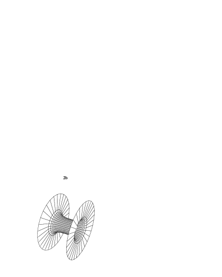
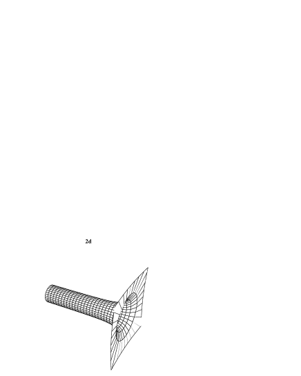
Figure 2: In (a) we have plotted the closed oscillating solution for $k=1$ and (b) is the wormhole solution for $k=-1$. Below are the both extremal limits: (c) corresponding to $R\times S_{k}^{3}$ and (d) the throat solution with one flat region for $k=-1$.

¿From the geometry it is clear that both extremal limits are non singular in the string frame. However, in the Einstein frame (41) is singular at certain points. If we calculate the Ricci scalar in the extremal limit we find

$$R_{E}\sim\frac{1}{|\sin\sqrt{k}\eta\,\cos\sqrt{k}\eta|^{3}}\ .$$ (42)

Thus, corresponding to the zeros of the Weyl factor in (41) the Ricci scalar has singularities. The asymptotic behavior of the world radius in the proper time $\tau$ is: $a(\tau)\sim\tau^{\frac{1}{3}}$ for $\tau\rightarrow 0$ (independently of $k$) and at infinity we obtain $a(\tau)\sim\sqrt{\tau}$ for $k=0$ and for $k=-1$ the metric (41) is again asymptotically flat.

Finally, let us discuss what happens if we perform the extremal limit. We have plotted the results in figures (2a-2d). For $k=1$ in the limit (11) the maxima and minima approach each other yielding a 4d $R\times S^{3}$ geometry which is a static universe (figure (2c)). In the case of $k=-1$ the solution has two asymptotic flat regions connected by a wormhole (figure (2b)). In this case we have two possibilities to perform the extremal limit. The limit (11) shifts both flat regions to the infinite past or infinite future and we have again a static universe with the only difference that $S^{3}$ has to be replaced by the 3d pseudo sphere. In the other extremal limit one flat region remains fixed and the other one is shifted to infinity. Looking on (40) one could think that there are two flat regions ($\eta\rightarrow\pm\infty$), but from every point $\eta_{0}$ (positive or negative) the point $\eta=0$ is infinite far away

$$s=\int_{\eta_{0}}^{\eta}\sqrt{\tilde{\eta}^{2}+t_{-}^{2}}\,\frac{d\tilde{\eta}}{\tilde{\eta}}=\left[\sqrt{\tilde{\eta}^{2}+t_{-}^{2}}-t_{-}\log\frac{\sqrt{\tilde{\eta}^{2}+t_{-}^{2}}+t_{-}}{|\tilde{\eta}|}\right]_{\eta_{0}}^{\eta}\longrightarrow\infty\quad\mbox{for}\quad\eta\rightarrow 0$$ (43)

and therewith the other flat region is not reachable. Asymptotically one can reach one flat region ($\eta\rightarrow\infty$ if $\eta_{0}>0$; see figure (2d)) or the point $\eta=0$ (corresponding to minimal extension of the throat). In both cases an infinite proper time is necessary. As long as we are not in the extremal limit the corresponding length is finite. Thus, the wormhole solution for $k=-1$ loses during the extremal limit one or both of its flat regions.

Additional dust contribution: Finally, we want to discuss whether it is possible to include dust matter in a consistent way. In [13, 12] it was argued that the 4d cosmological interpretation of a ($k=+1$) 5d back hole solution is pathological. Namely, an additional dust contribution to the energy momentum tensor would create a singularity near the maximal extension of the universe. Let us investigate whether a similar effect occurs here, too. For that reason we consider our 5d solution in the Einstein frame and perform a time transformation to get the standard Schwarzschild metric (3) (note, that here the functions $\lambda(t)$ and $\rho(t)$ do coincide with the solution given in (6)). An additional dust contribution to the 5d energy momentum tensor is given by

$$T_{tt}=\mu(t)\,e^{\lambda}\ .$$ (44)

Assuming that for the dust part of the energy momentum tensor the energy conservation is fulfilled we find for the energy density

$$\mu(t)=\frac{C}{\rho\,t^{3}}\ .$$ (45)

Because the dust part of the energy momentum tensor contributes to the $(t,t)$ part only the function $\lambda(t)$ remains unchanged ($\lambda$ is defined by the (5,5) component of the Einstein equation). The $(t,t)$ part of the Einstein equation yields a modified function $\rho(t)$

$$\rho=\left(1+C\,\frac{2}{3}\int^{t}\frac{(1-\frac{1}{3}(\frac{t_{-}}{\tilde{t}})^{2})d\tilde{t}}{[(-k+(\frac{t_{+}}{\tilde{t}})^{2})(1-(\frac{t_{-}}{\tilde{t}})^{2})]^{\frac{2}{3}}\,\tilde{t}^{2}}\right)\tilde{\rho}(t)$$ (46)

where $\tilde{\rho}$ is the compactification radius (modulus field) when the dust contribution to the energy momentum tensor vanishes ($C=0$). We want to restrict ourselves on regions away from the point of minimal extension ($\tilde{t}^{2}=t_{-}^{2}$). Obviously, the dust contribution (44) is singular at zeros of $\rho$. As long as $C>0$ the zeros of $\rho$ coincide with the zeros of $\tilde{\rho}$ and the dust part yields no additional divergencies. But if $C<0$ additional zeros can occur. For $k=0,-1$ the integral is finite and as long as $|C|$ is smaller than a critical value nothing disastrous happens (it is reasonable to restrict oneself on small perturbations). For $k=1$, however, the integral is divergent if we approach the maximal extension of the 4d string metric $\tilde{t}^{2}=t_{+}^{2}$ and for all negative $C$ we get an additional zero of $\rho$. Since this point is a singularity or horizon of the 5d theory this behavior is not surprising. Some confusion can appear after reduction to 4d because the 4d string metric is completely smooth. But nevertheless at this point the scalar matter part (dilaton and modulus) has singularities and one can expect that also the dust matter part is singular there. In the 4d Einstein frame are no such shortcomings because all zeros of $\rho$ and therewith singularities in the energy momentum tensor are accompanied by curvature singularities. Sokolowski [30] argued that just this behavior indicates that in this context the Einstein frame is physically more reasonable. Thus, we can conclude that dust matter can be included consistently as long as we are not too close to the extrema in the string frame or equivalently not to close to the curvature singularities in the Einstein frame.

5 Conclusions

In the present paper we discussed a combination of string and Kaluza–Klein theory [6] in the context of cosmological space time structures. For that sake we had to generalize the 5d black hole solution [15, 16] to arbitrary constant curvature of the spherical 3d subspace. Furthermore we had to interchange the signature of time and radius in order to get a cosmological solution after the Kaluza–Klein reduction.

We were able to show that the 5d solution generalized to arbitrary constant spatial curvature possesses a limit where it is exact to all orders in $\alpha^{\prime}$. That was done in analogy to the considerations in [17]. So, at least in a certain limit there is an exact conformal field theory behind our 5d phenomenological solution.

After performing the Kaluza–Klein reduction we got a four dimensional configuration with an isotropic cosmological metric, a dilaton field, torsion and a modulus field. Unfortunately there is no way to find an analytical expression for the metric in the standard Robertson–Walker form. That form is very suitable for the discussion of cosmological scenarios. Therefore it is worthwhile to give a numerical solution for the world radius. For certain special cases one can find analytical results. However, in those special cases the dilaton and the torsion of the 5d theory vanish and hence we get the result known from Einstein gravity [12]. Depending on the choice of parameters we have finite or infinite universes. For $t_{\pm}^{2}>0$ our cosmological solution is oscillating for $k=1$, for $k=-1$ we get a wormhole solution with two flat regions (in the infinite past and in the infinite future), for $k=0$ the geometry is also a wormhole but without flat regions. Transforming these solutions into the Einstein frame has the consequence that the wormholes and all other extrema of the string frame shrink to zero and form singularities. In some sense the singularities in both frames are complementary: a singularity in one frame is an (non singular) extremum in the other frame. The reason is, that the dilaton is divergent at all zeros and extrema of the world radius. In addition, we have briefly discussed the question whether matter or information can pass the wormhole. In this region the 5d metric has a smooth 3d spherical part and a singular 2d BH part and for winding modes it is possible to pass the 2d BH singularity. In addition to the numerical results the time dependence of the world radius was given in some asymptotical regions.

Finally we discussed the question what happens when we throw dust into the five dimensional space time. For that we transformed the 5d effective string action to the Einstein frame and added a dust contribution to Einstein’s equations. We observed that for open universes ($k=0,-1$) there will be no additional singularity in the dust contribution as long as it does not exceed a critical value. For closed universes ($k=1$) the dust contribution becomes singular near the maximal extension of the universe in the string frame. But because at this point the dilaton is divergent too, this singular matter contribution is not surprising. Instead, transforming the solution into the Einstein frame yields the result that all divergencies in the matter contribution coincide with divergencies of the metric (at the big bang or the big crunch).

The most interesting open question in our approach is whether it is possible to find exact 5d (or higher dimensional) solutions which will give a cosmological solution after Kaluza–Klein reduction. For closed universes those exact solutions might be obtained by the consideration of gauged WZW models consisting of a group which has the $SU(2)$ as a subgroup. However, the gauging must not affect the $SU(2)$ subgroup in order to preserve the $S_{3}$ geometry. Perhaps those solutions will also be interesting in the context of black hole physics, (as the one we used obviously was).

Acknowledgments
S. F. would like to thank Amit Giveon and Gautam Sengupta for useful discussions. K. B. is grateful to J. Garcia–Bellido, L. Dixon, L. Susskind, A.A. Tseytlin and D.L. Wiltshire for helpful discussions and remarks.

References

- [1] S. W. Hawking,Comm. math. Phys. 43(1975)199;
- [2] J. A. Harvey, A. Strominger: “Quantum Aspects of Black Holes”, Trieste Lectures 1992, EFI-92-41 (hep-th/9209055);
- [3] I. Antoniadis, C. Bachas, J. Ellis, D.V. Nanopoulos, Nucl. Phys. B328 (1989) 117;
-
[4]
C. R. Nappi, E. Witten, Phys. Lett. B293(1992)309;
A. Giveon, A. Pasquinucci, Phys. Lett. B294(1992)162; - [5] K. Behrndt, S. Förste, Phys. Lett. B320(1994)253;
-
[6]
T. Banks, M. Dine, H. Dijkstra, W. Fischler,
Phys. Lett. B212(1988)45,
J. Maharane, J.H. Schwarz, Nucl. Phys. B390(1993)3; - [7] A.A. Tseytlin, Int.J.Mod.Phys. D1 (1992) 223;
- [8] A.A. Tseytlin, in procc. of “String quantum gravity and physics at planck energy scale”, Erice, 1992 (hep-th: 9206067);
-
[9]
D. Lüst: “Cosmological String Background”, CERN-TH.6850/93
(hep-th: 9303175); - [10] M. Gasperini, G. Veneziano: “Inflation, deflation, and frame independence in string cosmology”, Mod. Phys. Lett. A8 (1993) 3701;
-
[11]
D.S. Goldwirth, M.J. Perry: “String-dominated cosmology”,
CFA–3694
(hep-th: 9308023); - [12] R.A. Matzner, A. Mezzacappa, Phys. Rev. D32(1985)3114;
- [13] D.L. Wiltshire, Phys. Rev. D36(1987)1634;
- [14] G.W. Gibbons, P.K. Townsend, Nucl. Phys. B282(1987)610;
- [15] G.W. Gibbons, K. Maeda, Nucl. Phys. B298 (1988) 741;
- [16] G.T. Horowitz, A. Strominger, Nucl. Phys. B360 (1991) 197;
- [17] S.B. Giddings, A. Strominger, Phys. Rev. Lett. 61 (1991) 2930;
-
[18]
E. Braaten, T.L. Curtright, C.K. Zachos, Nucl. Phys. B260;
(1985)630
S. Mukhi, Phys. Lett. B162(1985)345; - [19] E. Witten, Comm.Math.Phys. 92(1984) 455 ;
- [20] E. Witten, Phys. Rev. D44(1991)314 ;
- [21] A. Giveon, Mod.Phys.Lett. A6 (1991) 2843;
- [22] R. Dijkgraaf, H. Verlinde, E. Verlinde, Nucl. Phys. B371 (1992) 269;
- [23] C.G. Callan, J.H. Harvey, A. Strominger: ”Supersymmetric String Solitons”, Trieste Lectures 1991, EFI–91-66 (hep-th: 9112030);
- [24] T. Buscher, Phys. Lett. 194B(1987)59, Phys. Lett. 201B(1988)466;
- [25] K. Behrndt, S. Förste, preprint SLAC-PUB-6411 (hep-th: 9312167), to appear in procc. “27th Symposium on the Theory of Elementary Particles”, Wendisch–Rietz, 1993;
-
[26]
N. Sanchez, G. Veneziano, Nucl. Phys.B333 (1990) 253;
J. Garcia–Bellido, L.J. Garay,Nucl. Phys. B361 (1991) 713, Nucl. Phys.B400 (1993) 416; - [27] A.A. Tseytlin, Int.J.Mod.Phys.A3 (1988);
- [28] B.A. Campbell, A. Linde, K.A. Olive , Nucl. Phys. B355 (1991) 146;
- [29] R. M. Wald: General Relativity, Chicago & London 1984;
- [30] L.M. Sokolowski, Class.Quant.Grav. 6 (1989) 59.