Edge Asymptotics of Planar Electron Densities

Abstract

The $N\to\infty$ limit of the edges of finite planar electron densities is discussed for higher Landau levels. For full filling, the particle number is correlated with the magnetic flux, and hence with the boundary location, making the $N\to\infty$ limit more subtle at the edges than in the bulk. In the $n^{\rm th}$ Landau level, the density exhibits $n$ distinct steps at the edge, in both circular and rectangular samples. The boundary characteristics for individual Landau levels, and for successively filled Landau levels, are computed in an asymptotic expansion.

1 Introduction

Recent work [1, 2, 3, 4, 5, 6, 7] has illustrated the fundamental importance of the edge properties of planar incompressible quantum fluids in the understanding of the quantum Hall effect [8]. The physical incompressibility of the quantum Hall samples correlates boundary and bulk degrees of freedom in an interesting manner. The boundary values of the bulk particle densities behave as $1+1$ dimensional chiral Kac-Moody currents, the algebraic properties of which characterize the edge excitations [2, 3, 5]. Furthermore, the incompressibility may be fruitfully understood via a quantum deformation of the algebra of area-preserving diffeomorphisms [6, 7, 9]. Most of this work has concentrated on the physics of the lowest Landau level, but higher Landau levels are also important for a complete description of the quantum Hall effect. Here, I consider the exact large $N$ asymptotics of the edge properties of incompressible quantum fluids in higher Landau levels.

Consider the nonrelativistic Pauli hamiltonian operator for spin-polarized (i.e. scalar) fermions confined to the two-dimensional plane, in the presence of a uniform magnetic field (of strength B) perpendicular to the plane:

$$H={1\over 2m}\left(\vec{p}-{e\over c}\vec{A}\right)^{2}-{e\hbar B\over 2mc}$$ (1)

It is well known that, in the plane, the spectrum of this hamiltonian consists of an infinite discrete set of equally spaced energy levels (called ”Landau levels”), each of which is infinitely degenerate [10]. The infinite degeneracy of each level is directly related to the infinite area of the plane, and for a sample of finite area the degeneracy $N$ is of the order of the net magnetic flux $\phi$ through the region (measured in fundamental flux units $hc/e$):

$$N=\phi+\mu$$ (2)

where $\mu=O(1)$. In the plane, the eigenstates of the energy operator (1) may be written as $\psi_{n}^{j}$, where $n=0,1,2,\dots$ is the Landau level index (corresponding to the energy eigenvalue $E_{n}=n\hbar\omega_{c}$ where $\omega_{c}=eB/mc$ is the cyclotron frequency) and $j$ labels the degenerate states within each Landau level. In the $n^{th}$ Landau level, the expectation value of the density operator is given by the function

$$\rho_{n}(\vec{x})=\sum_{j}|\psi_{n}^{j}(\vec{x})|^{2}$$ (3)

For a fully filled Landau level, the occupation number equals the degeneracy, so the summation in (3) is always over $N$ values of $j$. At some fixed point $\vec{x}$ within the bulk of the sample, the thermodynamic limit, $N\to\infty$, simply involves extending this finite sum to an infinite sum. But at the edge of the sample, each individual density $|\psi_{n}^{j}(\vec{x})|^{2}$ in the sum is itself evaluated at a distance scale $|\vec{x}|=R$ which is correlated with the particle number as $R\sim\sqrt{\phi}\sim\sqrt{N}$ because of (2) and the condition of full filling. Thus the thermodynamic limit is much more subtle at the sample boundaries. The analysis of these limits is the subject of this paper.

The precise form of the eigenstates $\psi_{n}^{j}$ depends on the gauge chosen for the vector potential $\vec{A}$. To describe a finite sample, one should choose the gauge with the geometry of the sample boundary in mind. It is convenient to choose the gauge so that, on the boundary, the normal component of the vector potential $\vec{A}$ vanishes. Thus, for circular samples one uses the ”symmetric” gauge, $\vec{A}=-{B\over 2}(y,-x)$, while for rectangular samples (actually for rectangular strips with upper and lower sides identified) one uses the ”Landau” gauge, $\vec{A}=B(0,x)$. Owing to the degeneracy of the Landau levels, a change in the gauge involves a change in the nature of the sum over $j$ in (3), and so the functional form of $\rho_{n}$ is gauge dependent. We shall see that it is considerably easier to analyze the asymptotics of $\rho_{n}$ in the symmetric gauge than in the Landau gauge.

2 Circular Geometry

In the symmetric gauge it is useful to work with complex coordinates $z\equiv x+iy$, and the degenerate states are labelled by an (integer) angular momentum index $j$:

$$\psi_{n}^{j}={1\over\sqrt{\pi}}\left({B\over 2}\right)^{{j+1\over 2}}\sqrt{{n!\over(n+j)!}}~{}z^{j}~{}L_{n}^{j}\left({Br^{2}\over 2}\right)exp\left({-{Br^{2}\over 4}}\right)$$ (4)

In (4), the Landau level index $n$ runs over all nonnegative integers $n=0,1,2,\dots$, while the angular momentum index takes values $j=-n,-n+1,-n+2,\dots$ within the $n^{th}$ energy level. The $L_{n}^{j}$ are the generalized Laguerre polynomials [11] and the eigenstates $\psi_{n}^{j}$ are orthonormal in the plane. The individual densities $|\psi_{n}^{j}(\vec{x})|^{2}$ are radially symmetric functions of Gaussian form, peaked at a radius $r\simeq\sqrt{j+n}$, which increases with $j$. So for a finite disc of $N$ electrons, all in the $n^{th}$ Landau level, the density function is

$$\rho_{n}(\xi,N)=n!~{}e^{-\xi}\sum_{j=-n}^{N-n-1}{\xi^{j}\over(n+j)!}\left(L_{n}^{j}(\xi)\right)^{2}$$ (5)

where the natural dimensionless variable is $\xi={B\over 2}r^{2}$, in terms of which the boundary $r=R$ is given by $\xi={B\over 2}R^{2}\equiv\phi$. Thus, analysis of the boundary density in the thermodynamic limit involves the $N\to\infty$ behaviour of $\rho_{n}(\xi,N)$ for $\xi=\phi\simeq N$.

Consider first of all the density function for the lowest Landau level,

$$\rho_{0}(\xi,N) = e^{-\xi}\sum_{j=0}^{N-1}{\xi^{j}\over j!}$$ (6)

$$= e^{-\xi}e_{N-1}(\xi),$$

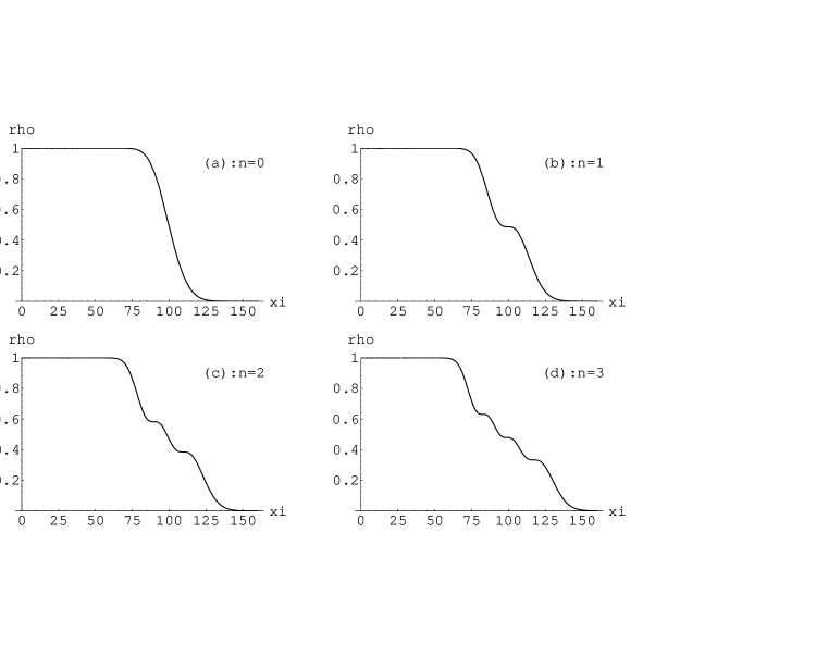
Figure 1: The symmetric gauge density functions (5) plotted for $N=100$ electrons for the first four Landau levels, $n=0,1,2,3$. Notice the uniform bulk density equal to $1$ and the boundary fall-off at $\xi\simeq N$. For the $n^{th}$ Landau level there are $n$ distinct steps at the boundary. The exact locations of these steps are given (see equation (15)) by the zeros of $L_{n}^{N-n-1}$ and $L_{n}^{N-n}$.

where $e_{N-1}(\xi)$ is the truncated exponential function [11]. This lowest Landau level density function is plotted in Figure (1 a) for $N=100$. We see that $\rho_{0}(\xi,N)$ does indeed represent a finite droplet of uniform bulk density (equal to 1 in the normalization chosen in equation (5)), dropping rapidly to zero at the ’edge’ where $\xi\simeq N$. For fixed $\xi$ within the bulk it is clear from (6) that $\rho_{0}(\xi,N)\to 1$ as $N\to\infty$. Indeed, since the bulk density is asymptotically uniform (see below), we can evaluate this uniform value deep in the bulk (i.e. at $\xi=0$) and (6) immediately gives $\rho_{0}(0,N)=1$.

To study $\rho_{0}(\xi,N)$ in the vicinity of the boundary (i.e. evaluated at $\xi=\phi=N-\mu$), we use the following integral representation [11] for the truncated exponential function in terms of the incomplete Gamma function $\Gamma(N,\xi)$

$$e_{N-1}(\xi)={\Gamma(N,\xi)\over\Gamma(N)}e^{\xi}$$ (7)

where

$$\Gamma(N,\xi)\equiv\int_{\xi}^{\infty}e^{-t}t^{N-1}dt$$ (8)

One can then use Laplace’s method [12] to show that the large $N$ behaviour near the edge is

$$\rho_{0}(N-\mu,N)={1\over 2}+{(\mu-{1\over 3})\over\sqrt{2\pi N}}+O({1\over N})$$ (9)

giving a leading order edge density equal to half the bulk density, with subleading corrections that go as $O({1\over\sqrt{N}})$ in the variable $\xi$. The $\xi$ derviative of the lowest Landau level density is

$${d\over d\xi}\rho_{0}=-{\xi^{N-{1}}\over(N-1)!}~{}e^{-\xi}$$ (10)

Note that the summation over $j$ has disappeared, due to cancellations between successive terms, a fact that makes the $N\to\infty$ limit of the derivative much easier to consider. For large $N$, the derivative is nonzero only in the vicinity of the boundary. In fact, for large $N$, all derivatives of $\rho_{0}$ vanish in the bulk, explaining the uniform bulk density. We can estimate the derivative ${d\over d\xi}\rho_{0}$ at the boundary using the fact

$${\xi^{N}\over N!}~{}e^{-\xi}={1\over\sqrt{2\pi N}}e^{-{(\xi-N)^{2}\over 2N}}\left(1-{1\over 12N}+\dots\right)\left(1+{1\over 3}{(\xi-N)^{3}\over N^{2}}+\dots\right)$$ (11)

Therefore,

$${d\over d\xi}\rho_{0}(N-\mu,N)=-{1\over\sqrt{2\pi N}}e^{-\mu^{2}/2N}\left(1+{\mu-1/12\over N}+\dots\right)$$ (12)

However, since the sample itself grows in size as $N$ increases ($R\sim\sqrt{N}$), it is more meaningful to consider the derivative in terms of the rescaled variable $\zeta=\xi/N$, for which the boundary is at $\zeta=(1-{\mu\over N})$. In terms of this rescaled coordinate,

$${d\over d\zeta}\rho_{0}|_{\zeta=1-\mu/N}=-\sqrt{{N\over 2\pi}}e^{-N(\mu/N)^{2}/2}\left(1+O({1\over N})\right)$$ (13)

which shows that the edge derivative becomes large and negative as $-\sqrt{N}$; and that the derivative is a delta function of width ${1\over{N}}$ concentrated at the boundary, as is appropriate for the derivative of a step-function density profile. In terms of the actual radial coordinate $r=\sqrt{{2\over B}\xi}$, the slope at the boundary is asymptotically constant

$${d\over dr}\rho_{0}\big{|}_{\rm boundary}=-\sqrt{B\over\pi}\left(1+O({1\over N})\right)$$ (14)

These results for the lowest Landau level density are reassuring, but not particularly surprising. The $N\to\infty$ limit is greatly facilitated by the relation of $\rho_{0}(\xi,N)$ to the incomplete gamma function. Such a direct relation is not available for the higher Landau levels due to the appearance of the Laguerre polynomial factors in (5). However, the asymptotic edge behaviour is significantly more interesting for these higher Landau levels. In Figure (1), the densities $\rho_{n}$ are plotted for $n=0,1,2,3$ with $N=100$. The pattern is striking - each density function has uniform bulk value equal to unity, and each falls off at an edge located at $\xi\simeq N$, but the $n\geq 1$ densities exhibit a distinct step-like pattern. This is a general feature of $\rho_{n}(\xi,N)$ - there are exactly $n$ such steps in the vicinity of the boundary. However, if one looks more closely by magnifying the scale of $\rho_{n}$ considerably, these ”steps” are in fact pairs of a local minimum and a local maximum. The locations of these local minima and maxima may be identified as a result of the following remarkable identity which generalizes the formula (10):

$${d\over d\xi}\rho_{n}(\xi,N)=-n!e^{-\xi}{\xi^{N-n-1}\over(N-1)!}L_{n}^{N-n-1}(\xi)~{}L_{n}^{N-n}(\xi)$$ (15)

Note that, as in (10), taking the derivative of $\rho_{n}$ enables the removal of the summation over the angular momentum index: this is due to intricate cancellations between successive terms in the sum, using the recurrence and differential-difference relations of the Laguerre polynomials. From (15) we see that the ’troughs’ and ’peaks’ of each step are located at the zeros of $L_{n}^{N-n+1}(\xi)$ and $L_{n}^{N-n}(\xi)$. Each Laguerre factor in (15) is a polynomial of degree $n$ with $n$ real zeros, and, furthermore, their zeros are interwoven (and for a given $n$, the $k^{th}$ zero of $L_{n}^{j}$ increases with $j$ [11]), explaining the pairing of local maxima and minima which gives the impression of steps.

Perhaps even more remarkable than this step-like behaviour is the fact that when the density functions for successive Landau levels are summed, the boundary again becomes ”smooth” (i.e. the steps disappear). This is directly relevant for applications to the quantum Hall effect [8], where one is interested, for example, in the density for full filling of the first $p$ Landau levels:

$$\rho_{\rm total}^{(p)}(\xi,N)\equiv\sum_{n=0}^{p-1}\rho_{n}(\xi,N)$$ (16)

These fully filled densities are plotted in Figure (2) for $p=1,2,3,4$ and for $N=100$. Notice that the form of these density functions is once again like the lowest Landau level density function $\rho_{0}$ plotted in Figure (1 a). To explain this miraculous cancellation of the boundary steps, note first of all the following identity which relates the density in the $n^{th}$ level to the density in the $(n-1)^{th}$ level:

$$\rho_{n}(\xi,N)=\rho_{n-1}(\xi,N)-(n-1)!e^{-\xi}{\xi^{N-n}\over(N-1)!}L_{n}^{N-n}(\xi)L_{n-1}^{N-n}(\xi)$$ (17)

The second term on the right hand side is concentrated at the boundary, since it is a sum of terms like (11). Using this identity, it follows that

$$\rho_{\rm total}^{(p)}(\xi,N)=p~{}\rho_{0}(\xi,N)-{e^{-\xi}\over(N-1)!}\sum_{n=1}^{p-1}(p-n)(n-1)!\xi^{N-n}L_{n}^{N-n}(\xi)L_{n-1}^{N-n}(\xi)$$ (18)

Once again, the sum on the right hand side is concentrated at the boundary, while the bulk value is just $p$ (i.e., $p$ times the bulk value of $\rho_{0}$). For low values of $p$ it is easy to perform the finite sums in (18), yielding

$$\rho_{\rm total}^{(1)}(\xi,N) = \rho_{0}(\xi,N)$$

$$\rho_{\rm total}^{(2)}(\xi,N) = 2\rho_{0}(\xi,N)+e^{-\xi}{\xi^{N-1}\over(N-1)!}\left(\xi-N\right)$$

$$\rho_{\rm total}^{(3)}(\xi,N) = 3\rho_{0}(\xi,N)+e^{-\xi}{\xi^{N-2}\over 2(N-1)!}\left(\xi^{3}-(3N-5)\xi^{2}+N(3N-7)\xi-N(N-1)^{2}\right)$$

$$\rho_{\rm total}^{(4)}(\xi,N) = 4\rho_{0}(\xi,N)+e^{-\xi}{\xi^{N-3}\over 6(N-1)!}\left(\xi^{5}-(5N-8)\xi^{4}+(10N^{2}-30N+26)\xi^{3}\right.$$ (19)

$$\left.\hskip 72.26999pt-N(10N^{2}-42N+50)\xi^{2}+N(5N^{3}-26N^{2}+37N-16)\xi\right.$$

$$\left.\hskip 72.26999pt-N(N-1)^{2}(N-2)^{2}\right)$$

The edge contributions are all concentrated at the boundary, and despite the seemingly complicated expressions (19), they all have a common functional form - see Figure (3).

Thus, the leading behaviour of the density of $p$ fully filled Landau levels is identical to $p$ times the density of the fully filled lowest Landau level, with subleading corrections $\sim O(1/\sqrt{N})$ concentrated at the boundary. For full filling of the first few Landau levels, this subleading edge behaviour can be determined from (9) and (19):

$$\rho_{\rm total}^{(1)}(N-\mu,N) = {1\over 2}+{\mu-{1\over 3}\over\sqrt{2\pi N}}+O({1\over N})$$

$$\rho_{\rm total}^{(2)}(N-\mu,N) = 1+{\mu-{2\over 3}\over\sqrt{2\pi N}}+O({1\over N})$$

$$\rho_{\rm total}^{(3)}(N-\mu,N) = {3\over 2}+{{3\over 2}\mu-{3\over 2}\over\sqrt{2\pi N}}+O({1\over N})$$

$$\rho_{\rm total}^{(4)}(N-\mu,N) = 2+{{3\over 2}\mu-2\over\sqrt{2\pi N}}+O({1\over N})$$ (20)

The general formula for this subleading behaviour, for any $p$, is

$$\rho_{\rm total}^{(p)}(N-\mu,N) = {p\over 2}+{2\Gamma\left(\left[{p+1\over 2}\right]+{1\over 2}\right)\over\Gamma\left({1\over 2}\right)\Gamma\left(\left[{p+1\over 2}\right]\right)}\left({\mu-{p\over 3}\over\sqrt{2\pi N}}\right)+O({1\over N})$$ (21)

where $[{p+1\over 2}]$ denotes the integer part of ${p+1\over 2}$. Notice that the coefficient of ${\mu\over\sqrt{2\pi N}}$ for $p$ odd is equal to that for $p+1$.

The derivative of $\rho_{\rm total}^{(p)}$ is localized at the boundary, since

$${d\over d\xi}\rho_{\rm total}^{(p)}=-{e^{-\xi}\over(N-1)!}\sum_{n=0}^{p-1}n!\xi^{N-n-1}L_{n}^{N-n-1}(\xi)L_{n}^{N-n}(\xi)$$ (22)

For low values of $p$, this derivative is:

$${d\over d\xi}\rho_{\rm total}^{(1)} = -e^{-\xi}{\xi^{N-1}\over(N-1)!}$$

$${d\over d\xi}\rho_{\rm total}^{(2)} = -e^{-\xi}{\xi^{N-2}\over(N-1)!}\left(\xi^{2}-2(N-1)\xi+N(N-1)\right)$$

$${d\over d\xi}\rho_{\rm total}^{(3)} = -e^{-\xi}{\xi^{N-3}\over 2(N-1)!}\left(\xi^{4}-4(N-1)\xi^{3}+6(N-1)^{2}\xi^{2}-4N(N-1)(N-2)\xi\right.$$

$$\hskip 216.81pt\left.+N(N-1)^{2}(N-2)\right)$$

$${d\over d\xi}\rho_{\rm total}^{(4)} = -e^{-\xi}{\xi^{N-4}\over 6(N-1)!}\left(\xi^{6}-6(N-1)\xi^{5}-3(N-1)(5N-6)\xi^{4}\right.$$ (23)

$$\hskip 36.135pt\left.+4(N-1)(N-2)(5N-3)\xi^{3}-3N(N-1)(N-2)(5N-11)\xi^{2}\right.$$

$$\hskip 36.135pt\left.+6N(N-1)^{2}(N-2)(N-3)\xi-N(N-1)^{2}(N-2)^{2}(N-3)\right)$$

In terms of the radial coordinate, the asymptotic boundary slopes are

$${d\over dr}\rho_{\rm total}^{(1)}|^{\rm boundary} = -\sqrt{B\over\pi}\left(1+O({1\over N})\right)$$

$${d\over dr}\rho_{\rm total}^{(2)}|^{\rm boundary} = -\sqrt{B\over\pi}\left(1+O({1\over N})\right)$$

$${d\over dr}\rho_{\rm total}^{(3)}|^{\rm boundary} = -{3\over 2}\sqrt{B\over\pi}\left(1+O({1\over N})\right)$$

$${d\over dr}\rho_{\rm total}^{(4)}|^{\rm boundary} = -{3\over 2}\sqrt{B\over\pi}\left(1+O({1\over N})\right)$$ (24)

The general formula for the leading-order boundary slope is

$${d\over dr}\rho_{\rm total}^{(p)}|^{\rm boundary}=-\sqrt{{B\over\pi}}{2\Gamma\left(\left[{p+1\over 2}\right]+{1\over 2}\right)\over\Gamma\left({1\over 2}\right)\Gamma\left(\left[{p+1\over 2}\right]\right)}\left(1+O\left({1\over N}\right)\right)$$ (25)

where, as before, $[{p+1\over 2}]$ denotes the integer part of ${p+1\over 2}$. Notice that for $p$ odd the asymptotic boundary slope is equal to that for $p+1$. Note also that the leading dependence of the slope agrees with the $O(\mu/\sqrt{N})$ dependence of $\rho_{\rm total}^{(p)}(N-\mu,N)$ given in (20,21), as it must.

These results rely on such specific properties of the Laguerre polynomials, that it is not immediately clear whether these strange edge phenomena are some sort of side-effect of the symmetric gauge or of the circular nature of the samples. It is therefore instructive to consider also the boundary phenomena for the rectangular samples using the Landau gauge. Notice that the Landau and symmetric gauges are related by the gauge transformation $\vec{A}^{Landau}=\vec{A}^{symmetric}+\vec{\nabla}\lambda$ with gauge function $\lambda={B\over 2}xy$. Normally, in the absence of degeneracies, different gauges lead trivially to identical densities since the nondegenerate wavefunctions are simply related by a phase factor $e^{i\lambda}$. However, due to the degeneracy of the Landau levels, the gauge invariance only implies that $e^{i\lambda}\psi_{n}^{j,{}symmetric}$ is some linear combination of the $\psi_{n}^{k,{}Landau}$ with the same energy (i.e. with the same Landau level index $n$). The particular form of this linear combination is gauge dependent, and so the conversion of the density from one gauge to another is not such a straightforward matter.

3 Rectangular Geometry

In the Landau gauge, the eigenstates of the Pauli energy operator (1) are

$$\psi_{n}^{k}=e^{iky}\left({B\over\pi}\right)^{1/4}{1\over\sqrt{2^{n}n!}}H_{n}\left(\sqrt{B}(x-{k\over B})\right)exp\left(-{B\over 2}\left(x-{k\over B}\right)^{2}\right)$$ (26)

where, as in (4), the Landau level label $n=0,1,2,\dots$, but now the degenerate states are labelled by a continuous momentum index $k$. This continuous momentum label may be discretized by compactifying in the $y$ direction. That is, if we consider the infinite strip $-\infty<x<+\infty$, $0\leq y\leq L$ rather than the entire plane, then with periodic or anti-periodic boundary conditions in the $y$ direction, the momentum index $k$ takes values $k=({2\pi\over L})j$. Here, $j$ takes integer values for periodic boundary conditions, and half-odd-integer values for anti-periodic boundary conditions. The $H_{n}$ are the Hermite polynomials [11], and the wavefunctions $\psi_{n}^{k}$ are orthogonal in the infinite strip.

The individual densities $|\psi_{n}^{k}|^{2}$ are independent of the $y$ coordinate (just as in the symmetric gauge the individual densities are independent of the angular coordinate), and have a Gaussian form in the $x$ direction (analogous to the radial Gaussian form of the densities in the symmetric gauge) peaked at $x\simeq{k\over B}$. Thus, for a rectangular strip of finite extent in the $x$ direction, there are corresponding upper and lower bounds on the allowed values of the discrete momentum. For convenience of notation, we choose the sample to be a square: $-{L\over 2}\leq x\leq+{L\over 2}$, $0\leq y\leq L$, and use the rescaled $x$-coordinate, $\xi\equiv{BL\over 2\pi}x={\phi\over L}x$, in terms of which the boundaries lie at $\xi=\pm{\phi\over 2}$.

Then the density for the fully filled $n^{th}$ Landau level is

$$\rho_{n}(\xi,N)=\sqrt{{2\over\phi}}{1\over 2^{n}n!}\sum_{j=-N/2}^{N/2}e^{-2\pi(\xi-j)^{2}/\phi}\left(H_{n}\left(\sqrt{{2\pi\over\phi}}(\xi-j)\right)\right)^{2}$$ (27)

where the flux $\phi$ and the particle number $N$ are related as in (2) for full filling.

The density (27) is plotted in Figure (4) for the first four Landau levels for $N=40$ and $\phi\simeq N$. From these plots we observe the same behaviour as in the symmetric gauge. In the lowest Landau level, there is a uniform bulk density equal to 1, which drops rapidly to zero in the vicinity of the boundaries at $\xi=\pm{\phi\over 2}\simeq\pm{N\over 2}$. In the higher Landau levels there is once again distinct step-like behaviour at the edge - specifically, in the $n^{\rm th}$ Landau level there are $n$ distinct steps in the density in the vicinity of the boundaries. Moreover, when the densities for successive Landau levels are summed, as in (16), these boundary steps cancel out, leaving a smooth boundary density of the same form as the lowest Landau level case: see Figure (5).

It is much more difficult to prove rigorous results for the asymptotics of the Landau gauge $\rho_{n}(\xi,N)$ because there are no clear analogues of the Laguerre polynomial results (15,17) for the Hermite polynomials. However, the Christoffel-Darboux identity for the Hermite polynomials [11] implies the following finite sum formula:

$$\sum_{n=0}^{m}{(H_{n}(x))^{2}\over 2^{n}n!}={1\over 2^{m+1}m!}\left((H_{m+1}(x))^{2}-H_{m}(x)H_{m+2}(x)\right)$$ (28)

Applying this formula to the fully filled density $\rho_{\rm total}^{(p)}\equiv\sum_{n=0}^{p-1}\rho_{n}$ with $\rho_{n}$ as in (27) we see immediately that

$$\rho_{\rm total}^{(p)}=p\rho_{p}+\sqrt{{2\over\phi}}{1\over 2^{p}(p-1)!}\sum_{j=-N/2}^{N/2}e^{-2\pi(\xi-j)^{2}/\phi}H_{p-1}\left(\sqrt{{2\pi\over\phi}}(\xi-j)\right)H_{p+1}\left(\sqrt{{2\pi\over\phi}}(\xi-j)\right)$$ (29)

The summation term on the right hand side of (29) is concentrated on the boundary - the fact that it vanishes in the bulk can be seen most directly by noting that the orthogonality of the polynomials $H_{p-1}$ and $H_{p+1}$ ensures that the leading contribution to the Euler-MacLaurin formula [12] vanishes. Therefore, the bulk value of the fully filled density is asymptotically equal to $p$ times the bulk density of the $p^{th}$ Landau level. This bulk value (for any given Landau level) may be evaluated deep in the bulk at $\xi=0$ by applying the Euler-MacLaurin formula to $\rho_{n}(0,N)$

$$\rho_{n}(0,N) = \sqrt{{2\over\phi}}{1\over 2^{n}n!}\sum_{j=-N/2}^{N/2}e^{-2\pi j^{2}/\phi}\left(H_{n}\left(\sqrt{{2\pi\over\phi}}j\right)\right)^{2}$$ (30)

$$= \sqrt{{2\over\phi}}\left\{{1\over 2^{n}n!}\int_{-N/2}^{+N/2}dxe^{-2\pi x^{2}/\phi}\left(H_{n}\left(\sqrt{{2\pi\over\phi}}x\right)\right)^{2}\right.$$

$$\hskip 72.26999pt\left.+{1\over 2^{n}n!}e^{-2\pi(N/2)^{2}/\phi}\left(H_{n}\left(\sqrt{{2\pi\over\phi}}{N\over 2}\right)\right)^{2}+\dots\right\}$$

$$= 1+O\left({1\over\sqrt{N}}\right)$$

where we have used the fact that ${1\over\sqrt{2^{n}n!}}|e^{-x^{2}/2}H_{n}(x)|<k$ for all $x$ and $n$, where $k=1.086435...$ is Charlier’s number [11]. By a similar computation, now evaluating $\rho_{n}(\xi,N)$ at the edge where $\xi\simeq\pm{N\over 2}$, we find

$$\rho_{n}(\pm{N\over 2},N) = \sqrt{{2\over\phi}}{1\over 2^{n}n!}\sum_{j=-N/2}^{N/2}e^{-2\pi(j\mp N/2)^{2}/\phi}\left(H_{n}\left(\sqrt{{2\pi\over\phi}}(j\mp N/2)\right)\right)^{2}$$ (31)

$$= {1\over 2}+O\left({1\over\sqrt{N}}\right)$$

4 Conclusion

In this paper it has been shown that, in the $N\to\infty$ limit, the expectation value of the planar electron density for the $n^{th}$ Landau level exhibits $n$ distinct steps near the boundary. This has been shown in both the symmetric gauge (appropriate for circular samples) and in the Landau gauge (appropriate for rectangular samples), in order to dispel possible doubts that this is perhaps an artifact of the particular (gauge dependent) basis used for the degenerate subspaces. At first sight, such non-smooth boundary structure seems to be problematic for the usual [2, 3, 5, 7] identification of the boundary charge with a chiral Kac-Moody current. However, when successive Landau levels are filled these boundary steps cancel out, leaving a smooth boundary whose boundary characteristics have been computed exactly (see equations (21,25)). It is not a priori obvious, in this independent particle picture, that the densities for independent Landau levels must conspire to produce a smooth edge behaviour.

Having identified the boundary behaviour of the higher Landau level electron densities, it would now be interesting to consider the boundary currents within a given Landau level, as discussed, for example, in [9] for the lowest Landau level. Presumably, for successively filled Landau levels one obtains different representations of the $W_{1+\infty}$ algebra. It would be very interesting to learn whether there is any connection between the boundary steps of the $n^{th}$ Landau level density and the different ”boundaries” needed for the $W_{1+\infty}$ representation theory and for the fractional QHE hierarchy [2, 4, 6]. It should also be possible to apply some of the results obtained here, for the asymptotic behaviour of sums of Laguerre and Hermite polynomials, to the analysis of the pair correlation function [13] and to the Coulomb interaction energy in higher Landau levels.

Acknowledgements: I am grateful to C. Bender, A. Cappelli, A. Lerda, C. Trugenberger and G. Zemba for discussions relating to this problem. This work has been supported in part by the D.O.E. through grant number DE-FG02-92ER40716.00, and by the University of Connecticut Research Foundation.

Figure 2: The symmetric gauge density functions $\rho_{\rm total}^{(p)}(\xi,N)$ for $p$ fully filled Landau levels, plotted for $N=100$ electrons. Notice the uniform bulk density equal to $p$, the boundary density equal to ${p\over 2}$, and the absence of the boundary steps seen in the individual higher Landau level densities in Figure (1).

Figure 3: The $N=100$ edge contribution by which the symmetric gauge density for $p$ fully filled Landau levels differs from $p$ times the density for the lowest Landau level - see (18,19). Notice that the edge contribution is centered at $\xi\simeq 100$ and that for different $p$ it has the same functional form.

Figure 4: The Landau gauge density functions (27) plotted for $N=40$ electrons for the first four Landau levels, $n=0,1,2,3$. Notice the uniform bulk density equal to $1$ and the boundary fall-off at $\xi\simeq\pm{N\over 2}$. For the $n^{th}$ Landau level there are $n$ distinct steps at each boundary.

Figure 5: The Landau gauge density functions $\rho_{\rm total}^{(p)}(\xi,N)$ for $p$ fully filled Landau levels, plotted for $N=40$ electrons. Notice the uniform bulk density equal to $p$, the boundary density equal to ${p\over 2}$, and the absence of the boundary steps seen in the individual higher Landau level densities in Figure (4).

References

• [1] B.ย Halperin, Phys. Rev. B 25, 2185 (1982), Phys. Rev. Lett. 52, 1583 (1984), 52, 2390 (E) (1984).
• [2] X-G.ย Wen, Phys. Rev. Lett. 64, 2206 (1990), Int. Journ. Mod. Phys. B 6, 1711 (1992).
• [3] M.ย Stone, Ann. Phys. 207, 38 (1991), Phys. Rev. B 42, 8399 (1990).
• [4] J.ย Frรถhlich and A.ย Zee, Nucl. Phys. B 354, 369 (1991); X-G.ย Wen and A.ย Zee, Phys. Rev. B 46, 2290 (1993).
• [5] A.ย Cappelli, G.ย Dunne, C.ย Trugenberger and G.ย Zemba, Nucl.Phys. B 398, 531 (1993), โ€Symmetry Aspects and Finite-Size Scaling of Quantum Hall Fluidsโ€, CERN Preprint TH-6784/93, Proc. Conf. Common Trends in Condensed Matter and High Energy Physics, Chia Laguna (Italy), September 1992, ed. L.ย Alvarez-Gaumรฉ et al, to appear in Nucl. Phys. B (Proc. Suppl.).
• [6] A.ย Cappelli, C.ย Trugenberger and G.ย Zemba, Nucl. Phys. B 396, 465 (1993), Phys. Lett. B 306, 100 (1993), โ€Classification of Quantum Hall Universality Classes by $W_{1+\infty}$ Symmetryโ€, Max-Planck-Institut Preprint MPI-Ph/93-75 (October 1993).
• [7] S.ย Iso, D.ย Karabali and B.ย Sakita, Nucl. Phys. B 388, 700 (1992), Phys. Lett. B 296, 143 (1992).
• [8] For excellent reviews of the QHE, see: R.ย Prange and S.ย Girvin, The Quantum Hall Effect, Springer Verlag, New York (1990); M.ย Stone, Quantum Hall Effect, World Scientific, Singapore (1992).
• [9] J.ย Martinez and M.ย Stone, โ€Current Operators in the Lowest Landau Levelโ€, Santa Barbara Preprint NSF-ITP-93-38 (March 1993).
• [10] L.ย Landau, Zeit. Phys. 64, 629 (1930); L.ย Landau and E.ย Lifshitz, Quantum Mechanics (Nonrelativistic Theory), Pergamon Press, Oxford (1977).
• [11] A.ย Erdรฉlyi et al, Eds., The Bateman Manuscript Project, Volume II: Higher Transcendental Functions, Krieger Publishing Co., Malabar (FL) (1981).
• [12] C.ย Bender and S.ย Orszag, Advanced Mathematical Methods for Scientists and Engineers, McGraw-Hill, New York (1978).
• [13] A.ย MacDonald, Phys. Rev. B 30, 3550 (1984).
Refer to caption