Lattice models and $N=2$ supersymmetry

Abstract

We review the construction of exactly solvable lattice models whose continuum limits are $N=2$ supersymmetric models. Both critical and off-critical models are discussed. The approach we take is to first find lattice models with natural topological sectors, and then identify the continuum limits of these sectors with topologically twisted $N=2$ supersymmetric field theories. From this, we then describe how to recover the complete lattice versions of the $N=2$ supersymmetric field theories. We discuss a number of simple physical examples and we describe how to construct a broad class of models. We also give a brief review of the scattering matrices for the excitations of these models.

USC-93/026
          hep-th/9311138
         November, 1993

1 Introduction

$N=2$ supersymmetric theories in two dimensions are in some ways much simpler than their non-supersymmetric kin. This is essentially because the $N=2$ supersymmetry imples the presence of a topological sector for which semi-classical analysis yields exact quantum results. (In the language of supersymmetry, the “$F$-terms” are not renormalized.) This does not mean that the model is semi-classically rigid, but only that a key (topological) subsector of the theory is semi-classically determined: the complete theory is very rich and has all of the complexity of a non-supersymmetric theory. The topological subsector has thus provided a “bridgehead” from which many of the non-trivial quantum aspects of the model can be explored, and usually with greater facility, and often in more detail than is possible for non-supersymmetric theories. (For reviews, see [1, 2, 3].) For example, $N=2$ Landau-Ginzburg theories have a superpotential that is exact. For $N=2$ superconformal models this means that the operator algebra and the anomalous dimensions (conformal weights) of the Landau-Ginzburg fields are trivially computable [4, 5]. On the other hand, it is still somewhat unclear as to how much of the rest of the theory, and in particular, how much of the complete operator content is determined by the Landau-Ginzburg potential. Indicative results are known: For example, the ADE classification of modular invariants of $N=2$ minimal models collapses to the ADE classification of modality zero singularities [6, 4]. Ramond sector characters can be obtained from the Landau-Ginzburg potential by computing the elliptic genus [7, 8, 9, 10].

For $N=2$ supersymmetric quantum integrable field theories (QIFT’s ) the Landau-Ginzburg description leads to transparent analysis of the soliton structure [11, 12, 13]. In $N=2$ QIFT’s, and even non-integrable $N=2$ QFT’s, differential equations can also be obtained for some of the scaling functions [14]. For the $N=2$ QIFT’s these scaling functions can also be obtained from the thermodynamic Bethe ansatz, but instead of differential equations, one obtains complicated integral equations [15].

Over the last decade it has also become evident that many of the structures of quantum integrable field theories have analogues in exactly solvable lattice models (see, for example [16, 17, 18, 19, 20]). Using this technology, lattice models have been constructed in which the continuum limits give rise to many of the non-supersymmetric conformal field theories. It is therefore natural to expect that there should be exactly solvable lattice models whose continuum limits are $N=2$ supersymmetric QIFT’s. We shall henceforth refer to such lattice models as $N=2$ lattice models. It is also to be hoped that such lattice regularizations may have especially simple features. If so, they may in turn help us to understand some mysterious issues like the appearance of branching functions in local height probabilities [21]. There are also practical reasons for constructing $N=2$ lattice models. The simplicity of $N=2$ QFT’s has led to more progress than in any other kind of field theory. It is especially attractive to try to compare some of the advanced results with real or computer experiments. To do so, the construction of a “physically reasonable” lattice model whose continuum limit is the $N=2$ QFT of interest is a natural way to proceed. We also hope that the $N=2$ lattice models will be “more universal” than their non-supersymmetric counterparts. Indeed, consider a general non-supersymmetric model, and suppose that we do not impose the requirement of exact solvability. Since there are generically very many relevant operators in such a model, the corresponding coupling constants would need to be very finely tuned in order to find a particular second order phase transition and hence a particular conformal field theory. Thus one of the side-effects of exact solvability is to automatically make such a fine-tuning of the couplings. The $N=2$ lattice models have a further special, and robust, identifying feature: the presence of a topological sector. Thus, not only can one construct them by imposing exact solvability, but one can also identify them by virtue of their topological sector. In fact, we will argue in this review that any “trivial” statistical mechanics model will probably give rise to a non-trivial $N=2$ lattice model, and thus the $N=2$ models will be of relevance in a large variety of situations. For instance the polymer and percolation problems, the statistics of Bloch walls in high temperature Ising model, Brownian motion, are all described by $N=2$ supersymmetric theories.

The investigation of lattice models associated with supersymmetric QFT’s has a rather long history. To our knowledge it started with the study of $N=1$ supersymmetry in the tricritical Ising model [22, 23, 24] and the fully frustrated XY-model [25] (the latter related to Josephson junctions arrays).

Then $N=1$ supersymmetry together with $N=2$ supersymmetry were observed at some special points of the Ashkin-Teller model and the six-vertex (or XXZ) model [26, 27, 28]. By analysis of torus partition functions it was easy to identify more generally special points of the higher spin $U_{q}(SU(2))$ vertex models [29, 30] that were $N=2$ supersymmetric. A physical explanation of this came later [31]. In the simplest case of the six-vertex model it leads to $N=2$ supersymmetry in the percolation problem. Similarly, by analysis of the related Izergin-Korepin ($O(n)$) model [32, 33], another family of lattice models with $N=2$ supersymmetry was found (or conjectured). The simplest of this family leads to $N=2$ supersymmetry in the self-avoiding walk (polymer) problem. This turns out to be a very favorable case for comparison with real and numerical experiments [34]. More complete study of the $SU(2)$ based models was carried out in [35]. Recently, it has been shown how one can go beyond models based upon $SU(2)$. That is, $N=2$ lattice models based on any simply-laced Lie algebra have been constructed by using “partial restriction” of modified solid-on-solid (SOS) models, or equivalently by twisting and performing partial quantum group truncation of the corresponding vertex models. The continuum limits of these lattice models are the $N=2$ superconformal coset models based on hermitian symmetric space [36, 37, 38].

At the present time, there is a respectable number of known $N=2$ lattice models. They resemble in some respects the corresponding QFT, although the structures are not yet as closely linked as one would wish. They have already led to comparison with real and numerical experiments, and very good agreement has been found. The purpose of this review is to describe in some detail the current state of knowledge and to point to new directions of research.

The first section is rather qualitative and collects observations about the expected structure of $N=2$ lattice models. A variety of simple examples is worked out, starting from simple geometrical ideas and introducing the fundamental tools that will be used extensively later. One of the basic themes underlying the $N=2$ lattice constructions is the role of the “trivial” topological sector. This will be used directly in later sections to construct and analyse the $N=2$ lattice models based on general Lie algebras. In the fourth section we will briefly discuss the scattering matrices of excitations in the $N=2$ lattice models and their continuum limits. In section five we discuss further physically interesting aspects of $N=2$ lattice models, and in the last section we conclude by summarizing what we believe are the important open problems in the subject.

2 Features of $N=2$ lattice models.

Our purpose in this section is to study a number of closely related and simple models that exhibit the basic features of the $N=2$ lattice models. Our aim is to try to give some intuitive understanding of $N=2$ lattice models, to show how one can analyse their various features, and ultimately to evolve a strategy for finding such models.

2.1 The clues from the topological sector

If the theory has $N=2$ supersymmetry then, as mentionned earlier, there is a topological sector, with the following characteristics. The topological sector of the $N=2$ QFT consists of operators that are annihilated by two of the four supercharges. The topological physical states consist of only the ground states of the non-topological $N=2$ lattice model. The operators of the topological model are order parameters of the non-topological sector, and the correlation functions of these operators are constant in the topological sector.

The presence of some sort of “topological” sector is one of the main attributes of an $N=2$ lattice model, and because of the links between the topological and non-topological sectors in the continuum, the identification of the lattice topological sector proves an important tool in the construction of the complete $N=2$ lattice model. More precisely, the idea is to study representations of the lattice algebras and lattice symmetries (such as Temperly-Lieb and quantum group representaions). For certain choices of parameters some of these will be very simple or trivial, and the corresponding lattice models will be “topological.” The idea is to define the topological model precisely, fix the parameters to their topological values, but then modify the choice of representations or modify the choice of lattice variables in such a manner that the $N=2$ lattice model emerges from its topological limit. We will describe two “dual” methods for accomplishing this. The first relies on the fact that a lattice model can have very different properties when it is described by different sets of observables that are not mutually local. One thus obtains some of the $N=2$ lattice models by considering a “trivial” model where the given lattice variables do not interact, and then one makes a “change of variables” to new set of geometrical observables that have highly non-trivial properties. The non-interacting observables describe the topological model, while the new observables describe the non-trivial $N=2$ lattice model. The second method is to consider the restriction process in solid-on-solid (SOS) models (or quantum group truncation in the equivalent vertex formulation), and start with a restriction that results in a “frozen” or completely rigid topological model. One then “gets something from nothing” by relaxing the restrictions imposed on the SOS model, while at the same time one “topologically untwists” the Boltzmann weights to avoid singularities in the transfer matrix. It turns out that the first method is a priori a little more intuitive, while the second method is much easier to generalize. We therefore start by describing a simple example of the first procedure and then trace a connection to the second method.

2.2 Examples of lattice topological sectors

2.2.1 Percolation: an example of a geometrical model

Consider a square lattice and put on every edge a variable $\sigma$ that can take two possible values, $0$ or $1$. Suppose that the edge variables do not interact with each other, but put the whole system in a magnetic field. Since the spins do not interact, all correlation functions are trivially constant (or, at least are delta functions). This appears to be a completely trivial model and the partition function is ${\cal Z}=\left(1+e^{-H}\right)^{N_{E}}$, where ${N_{E}}$ is the number of edges. We now pass to a new set of observables (called geometrical observables in what follows): Call edges with variable $\sigma=0$ “empty” and edges with variable $\sigma=1$ “occupied” (we represent occupied edges with heavy lines in figure 1) and consider the geometrical properties of clusters, that is, of the connected sets of occupied edges. These cluster observables are non-local with respect to the original $\sigma$ variables, and the “trivial” model now describes the bond percolation problem. Since the sum over variables $\sigma=0,1$ is unconstrained, there is a probability of $p={e^{-H}\over 1+e^{-H}}$ of having an occupied edge, and a probability of $p={1\over 1+e^{-H}}$ of having an empty edge. The correlation functions of new variables, such as the probability that two vertices belong to the same cluster, are non-trivial. The original trivial model can, of course, be recovered by deciding to study only local questions like “is this edge occupied” and forgetting about non local questions like “are these two edges part of the same cluster”. As we will see, the distinction between these two questions is clearer from a representation theory point of view, and easy to implement, for instance, in a transfer matrix formalism.

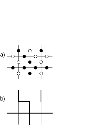
Figure 1: a) A configuration of “up” (black dot) or “down” (white dot) spins on the edges of the square lattice. b) The corresponding configuration of “occupied” or “empty” edges.

To determine the supersymmetry point of this model we consider it upon a torus. The new observables can be given various boundary conditions: for instance, one can sum over non-contractible clusters giving each some weight, or fugacity. The presence of unbroken supersymmetry means that, in the thermodynamic limit, the free energy per edge cannot depend upon the boundary conditions on the torus. Intuitively, if $p>1/2$ or $p<1/2$, one will find large clusters of occupied or unoccupied edges. Thus non-contractible clusters will make significant contributions to the free energy, and thus the latter will depend upon the boundary conditions. However, when one has $p=1/2$, or $H=0$, one is at the percolation point, a critical point where the geometrical correlation functions decay algebraically and there is a vanishing fraction of big clusters of occupied or unoccupied edges. The partition function is ${\cal Z}=2^{N_{E}}$. This lattice partition function is, as usual, defined up to a non-universal term of the form $e^{fN_{E}}$. In the continuum, the partition function simply counts the number of “different observables” of the model. It is rather reasonable that there is only one such observable (beside the identity): the variable $\sigma$. One thus expects $Z=2$. This is also consistent with the identification of this percolation problem as an $N=2$ lattice model. As we will see, the foregoing lattice partition function can be interpreted as the Witten index of the $N=2$ lattice model. We will soon present rather more direct evidence that for $p=1/2$ this is indeed an $N=2$ lattice model.

2.2.2 The dual point of view: the “frozen” Potts model

The foregoing non-trivial bond percolation problem can also be described using the $Q$-state Potts model in the limit $Q\to 1$. The general $Q$-state Potts model is defined by putting a spin variable, $\sigma$, on each vertex of the square lattice. These spin variables take values in $1,\ldots,Q$, and the lattice partition function is

$${\cal Z}_{\rm Potts}~{}=~{}\sum_{\{\sigma\}}\prod_{<i;j>}{}~{}e^{K~{}\delta(\sigma_{i},\sigma_{j})}\ ,$$ (1)

where the sum is over all spins and the product is over is over nearest neighbours. The connection with the percolation problem becomes evident upon making a high temperature expansion of the Potts model: The partition function can be written

$$Z_{\rm Potts}~{}=~{}{\rm tr}~{}\left(\prod_{<i;j>}\left\{1~{}+~{}(e^{K}-1)\delta(\sigma_{i},\sigma_{j})\right\}\right)\ ,$$ (2)

which can then be expanded graphically by connecting all vertices with the same spin $\sigma$. One then finds that

$$Z~{}=~{}\sum_{\rm graphs}(e^{K}-1)^{N_{B}}~{}Q^{N_{C}}\ ,$$ (3)

where $N_{B}$ is the number of bonds in the graph, and $N_{C}$ is the number of clusters. This high temperature expansion coincides with the bond percolation problem only if the $Q^{N_{C}}$ term is equal to one, i.e. if and only if $Q=1$. One must also make the following identification:

$$e^{K}-1~{}=~{}e^{-H}\ .$$ (4)

However, if one considers the Potts model with $Q=1$, one finds that it is a trivial, completely frozen, “topological” model. The partition function (1) collapses to ${\cal Z}_{\rm Potts}=e^{KN_{E}}$. The bond percolation problem should really be viewed as the $Q\to 1$ limit of the Potts model. For example, the derivatives of ${\cal Z}_{\rm Potts}$ at $Q=1$ describe generating functions for the percolation problem [39]. Similarly, derivatives of the Green functions correspond to geometrical correlation functions; for example the spin-spin two point function of the Potts model yields the probability that two vertices belong to the same cluster.

We therefore see that the percolation problem is closely associated with a frozen model. To obtain the non-trivial model from the frozen model we need to find models that are “close to the frozen model.” The natural way of doing this is to use an algebraic approach.

2.2.3 Representations of the Temperley-Lieb algebra

To proceed further it is convenient to think in algebraic terms and turn to a transfer matrix formalism [40]. Consider thus a rectangle of size $L\times T$ and propagation in the $\hat{y}$ direction. We define more precisely the geometrical observables in terms of connectivities as follows. Number the vertices on a given time slice by $1,2,\ldots,L$, running from left to right. The space of states ${\cal H}_{L}^{\rm geom}$ is the set of all possible partitions of $1,2,\ldots,L$. In a partition of $L$ at time $t$, two vertices are grouped together if at time $t$ they are connected through a cluster that extends into their present and past. For instance, for $L=4$ the partition $(13)(2)(4)$ correspond to the fact that there is connectivity between $1$ and $3$, while $2$ and $4$ are not currently connected to any other vertex by connections through clusters in their past (see figure 2). Introduce operators, $e_{k}$, that act on ${\cal H}_{L}^{\rm geom}$. For odd subscripts, $e_{2j-1}$ transforms connectivities at time $t$ to connectivities at time $t+1$ by inserting vertical “occupied” bonds at all but the $j^{\rm th}$ vertex. Thus one has $e_{3}|(13)(2)(4)>=|(13)(2)(4)>$, and $e_{1}|(13)(2)(4)>=|(1)(2)(3)(4)>$. For even subscripts, $e_{2j}$, modifies connectivities at the same time, and simply inserts a horizontal edge between the $j^{\rm th}$ and $(j+1)^{\rm th}$ vertices. For example, one has $e_{2}|(13)(2)(4)>=|(123)(4)>$.

Figure 2: The partition $(13)24$ means that vertices 1 and 3 are connected through a path of occupied edges at previous times (by convention past means edges below $y=t$). Acting with $e_{3}$ corresponds to adding an occupied vertical edge in all but the second column between $y=t$ and $y=t+1$ resulting again in $(13)24$. Acting with $e_{1}$ corresponds to adding an occupied vertical edge in all but the first column between $y=t$ and $y=t+1$ and this destroys the connection between vertices 1 and 3, resulting in the partition $1234$.

These operators satisfy the relations

$$e_{j}^{2}=\sqrt{Q}e_{j},\qquad e_{j}e_{j\pm 1}e_{j}=e_{j},\qquad[e_{j},e_{k}]=0,\ |j-k|\geq 2$$ (5)

with $\sqrt{Q}=1$, and hence furnish a particular representation of the Temperley-Lieb algebra [41, 42, 33]. The general form of this algebra can be realized in a number of simple models, and, in particular,in the $Q$-state Potts model.

Define ${\cal H}_{L}^{\rm Potts}$ to be the space of all possible (Potts model) spin states on the $L$ vertices across a time slice of the lattice. Introduce the following operators on ${\cal H}_{L}^{\rm Potts}$:

$$\left(e_{2j}\right)_{\sigma,\sigma^{\prime}}=\sqrt{Q}~{}\prod_{k}~{}\delta(\sigma_{k},\sigma_{k}^{\prime}){}~{}\delta(\sigma_{j},\sigma_{j+1})$$ (6)

and

$$\left(e_{2j-1}\right)_{\sigma,\sigma^{\prime}}={1\over\sqrt{Q}}~{}\prod_{k\neq j}~{}\delta(\sigma_{k},\sigma_{k}^{\prime})\ .$$ (7)

The operators $e_{j}$ satisfy the Temperly-Lieb algebra for general $Q$. The transfer matrix of the Potts model may be written:

$$\tau=Q^{L/2}\prod_{j=1}^{L}X_{2j}\prod_{j=1}^{L}X_{2j-1}$$ (8)

where

$$X_{2j-1}={e^{K}-1\over\sqrt{Q}}+e_{2j-1},\ X_{2j}=1+{e^{K}-1\over\sqrt{Q}}e_{2j}\ {}.$$ (9)

The decoupled spin model in the magnetic field is related to this by setting $Q=1$ and $e^{K}=1+e^{-H}$ as in (4). The transfer matrix of the bond percolation problem is also given by (8), (9), but with the Temperley-Lieb representation given at the beginning of this subsection. More generally the transfer matrices of the vertex and RSOS models that will soon be described, also read as in (8) and (9) but with their own Temperley-Lieb representation.

On a torus, the algebraic structure is slightly more complicated due to the additional edge between the first and $L^{\rm th}$ vertex. The correct algebra is now the periodic Temperley-Lieb algebra. The various possible weights associated to non-contractible clusters and the various natural geometrical sectors have precise meaning in terms of traces and representation theory [43].

2.3 Unfreezing frozen models

We believe that the foregoing features are generic for an $N=2$ lattice model. Such a model should be closely related to two trivial models: one rigid or frozen, and the other some kind of high temperature dual in which the lattice variables are decoupled from one another. In between these extremes is the Hilbert space of the $N=2$ lattice model. Common to all of these models is the representation theory of some underlying lattice algebra. The problem of making the $N=2$ lattice model is to find the proper observables in the decoupled model, or to find the proper “unfreezing” of the frozen model. As we will discuss, this may all be thought of in terms of choices of the representations of the lattice algebra. We will also find that while the “decoupled” description of the model is more intuitive, it is the “unfreezing” process that is easiest to implement more generally. To define more precisely the unfreezing procedure, we first want to describe two other representations of the Temperley-Lieb algebra, and their frozen limits.

2.3.1 Yet more frozen models

Consider the representation of the Temperley-Lieb algebra provided by restricted solid on solid (RSOS) models. (We refer to more general extensions of such models as interaction-round-a-face (IRF) models.) These representations have $\sqrt{Q}=2\cos\pi/(m+1)$, where $m$ is an integer. The model is defined by introducing heights, $\ell=1,\ldots,m$, on the vertices and faces of the original square lattice (figure 3). Represent these heights as the nodes of the Dynkin diagram of $A_{m}$. The transfer matrix now acts on a configuration space ${\cal H}_{2L}^{\rm RSOS}$ whose basis is given by elements $\{\ell_{j},j=1,\dots,L\}$ with the constraint that neighbouring vertices on the lattice carry heights that are neighbours on the $A_{m}$ diagram. Let $v_{\ell}$ be the components of the Perron-Frobenius eigenvector of the Cartan matrix of $A_{m}$ (or of the incidence matrix of the Dynkin diagram). That is, $v_{\ell}=sin(\pi\ell/(m+1))$. The representation of the Temperly-Lieb algebra is then given by:

$$\left(e_{j}\right)_{\ell\ell^{\prime}}~{}=~{}\delta(\ell_{j},\ell_{j+2}){}~{}{\left(v_{\ell_{j+1}}{}~{}v_{\ell^{\prime}_{j+1}}\right)^{1/2}\over v_{\ell_{j}}}~{}\prod_{k\neq j+1}\delta(\ell_{j},\ell^{\prime}_{j})\ .$$ (10)

The RSOS transfer matrix is then given by using this in (8) and (9). To get the representation with $Q=1$, one simply takes $m+1=3$. The model is rigid, with heights alternating between the value 1 on one sublattice, and the value 2 on the other. This model thus has two states, depending upon which sublattice takes the value 1 and which takes the value 2.

Figure 3: The RSOS variables are defined on the vertices of the diagonal lattice, that is the vertices and the faces of the original square lattice.

This model has some form of duality with the original non-interaction spin model. The non-interacting spin model can be considered as the $T\rightarrow\infty$ limit of an Ising model on the medial lattice. The dual [41] is an Ising model defined on the faces and vertices of the original lattice and at $T=0$, which is completely “frozen,” and has exactly two states.

More importantly for our current purposes, this model has an equivalent vertex formulation whose continuum limit is a Gaussian model. This will finally yield more direct evidence of the supersymmetry.

2.3.2 The vertex model and its continuum limits

We now introduce our final representation of the Temperley-Lieb algebra: the one provided by the six-vertex model. Introduce spin variables $\pm$ (usually represented by arrows) on the edges of the medial graph of the original square lattice (figure 4). Think of these spin variables as being basis vectors in $\,\hbox{$\vrule height=7.5pt,depth=-0.5pt,width=0.2pt\kern-2.29996pt{\rm C}$}^{2}$. The configuration space of the transfer matrix is now ${\cal H}_{2L}^{\rm vertex}=\left(\,\hbox{$\vrule height=7.5pt,depth=-0.5pt,width=0.2pt\kern-2.29996pt{\rm C}$}^{2}\right)^{2L}$. To define the operators $e_{j}$, introduce $4\times 4$ matrices $E_{ij,kl}$, where $i,j,k,l$ are either $+$ or $-$, by setting all the entries to zero, except the $ij$,$kl$ entry which is set equal to $1$. Then $e_{j}$ is equal to the identity in all but the $j^{\rm th}$ and $(j+1)^{\rm th}$ copies of $\,\hbox{$\vrule height=7.5pt,depth=-0.5pt,width=0.2pt\kern-2.29996pt{\rm C}$}^{2}$, where it is given by

$$e_{j}=q^{-1}E_{+-,+-}+qE_{-+,-+}-E_{+-,-+}-E_{-+,+-}\ .$$ (11)

The parameter $Q$ of the Potts model is related to the parameter $q$ of the six-vertex model by:

$$\sqrt{Q}~{}=~{}q+q^{-1}\ ,$$ (12)

and so the supersymmetric model corresponds to setting $q=\exp(i\pi/3)$.

Figure 4: The six-vertex arrows are defined on the edges of the diagonal (medial) lattice. They are also interpreted as domain walls for a SOS model whose heights are defined on the vertices and faces of the square lattice (see figure 3).

The continuum limit of this model is a Gaussian model [45, 18, 19]. More precisely, introduce variables $\phi$ on the vertices of the original lattice and in the middle of its faces, with values defined recursively by $\phi_{u}=\phi_{d}\pm 1$, that is, the value of $\phi$ above one edge of the medial equal to the value under it plus the value of the spin carried by the edge. The dynamics of these variables is described by a Gaussian action at large distance, and in the conventions where the topological defects are not renormalized, the action is

$$A~{}=~{}{g\over 4\pi}~{}\int~{}(\partial\phi)^{2}$$ (13)

with $g=2/3$. As a result, the partition function on a torus with doubly periodic boundary conditions,

$${\cal Z}~{}=~{}\hbox{tr}\left(~{}\tau^{\rm vertex}~{}\right)^{T}\ ,$$ (14)

is given, in the continuum, by

$$Z~{}=~{}Z_{G}(3/2)\ ,$$ (15)

where $Z_{G}$ is a Gaussian partition function. That is,

$$Z_{G}(g)~{}=~{}{1\over\eta\bar{\eta}}~{}\sum_{e,m\in Z}~{}p^{h_{em}/4}\bar{p}^{\bar{h}_{em}/4}\ ,$$ (16)

where

$$h_{em}~{}=~{}{1\over 4}\left({e\over\sqrt{g}}+m\sqrt{g}\right)^{2},\qquad\bar{h}_{em}~{}=~{}{1\over 4}\left({e\over\sqrt{g}}-m\sqrt{g}\right)^{2}$$ (17)

and $\eta(p)=p^{1/24}\prod(1-p^{n})$ is the Dedekind eta function, and the elliptic nome is given by $p=\exp-2\pi T/L$. Equation (15) coincides with the partition function of the first minimal (central charge $c=1$) $N=2$ superconformal model with projection on odd fermion number. The holomorphic generators of the $N=2$ superconformal algebra can be written (after normalizing the boson appropriately):

$$\begin{array}[]{lr}G^{+}(z)~{}=~{}e^{i\sqrt{3}\phi(z)}\ ;&G^{-}(z)~{}=~{}e^{-i\sqrt{3}\phi(z)}\ ;\\ J(z)~{}=~{}{i\over\sqrt{3}}\partial\phi(z)\ ;&T(z)~{}=~{}-{1\over 2}(\partial\phi(z))^{2}\ .\end{array}$$ (18)

If one used the trivial representation of the Temperley-Lieb algebra given by equations (6) and (7), instead of the representation given above, it would lead to

$${\cal Z}~{}=~{}\hbox{tr}\left(\tau^{\rm Potts}\right)^{T}~{}=~{}2^{N_{E}}\ .$$ (19)

In the continuum this partition function is, up to an overall normalization, the partition function in the Ramond sector with an insertion of $(-1)^{F}$, where $F$ is the fermion number. It is therefore constant and corresponds to the Witten index of the model. It may also be thought of as the partition function of the continuum topological matter model.

Beside partition functions, various physical observables in the percolation problem can be conveniently studied in the $N=2$ supersymmetry formalism. Usually the critical percolation problem is considered as a $c=0$ CFT, i.e. a twisted $N=2$ superconformal theory. The physical observables of statistical mechanics are then the ones that are usually discarded as unphysical from string theory point of view. The probability that two edges belong to the same cluster corresponds to an operator with half-integer labels in the Kac table of the $c=0$ CFT. Only by turning to an $N=2$ formalism can its correlation functions be studied. This operator belongs in the $N=2$ formalism to the sector “in between” Ramond and Neveu-Schwarz, with spatial boundary conditions twisted by $(\sqrt{-1})^{F}$. Its dimension in the twisted theory is $h={5\over 96}$.

2.3.3 A practical use of the topological sector

The identification of a topological sector is not only useful for supersymmetry purposes. If supersymmetry is unbroken, the free energy of a non-trivial lattice model, like the six-vertex model with $q=e^{i\pi/3}$, can be readily computed by turning to the topological frozen model. At the special supersymmetric point, it is not necessary to perform a Bethe ansatz computation to determine $f$. This will be discussed further in section 3.

2.3.4 Quantum group truncation, restriction and freezing

Because the six-vertex model (with free boundary conditions) has a quantum group symmetry, one can use this to reduce the Hilbert space of the model to obtain a new truncated model. In the language of height models this correspond to making the RSOS restriction. It may also be viewed as the lattice version of the BRST reduction of the Gaussian model to the Virasoro minimal models [44]. The first step is to take $q$ to be a root of unity. Here we will take $q=e^{i\pi/m+1}$, for some integer $m$. One then replaces the traces of operators by Markov traces, that is, the trace of an operator ${\cal O}$ is defined by:

$$tr_{M}({\cal O})~{}=~{}\hbox{tr}\left(~{}{\cal O}~{}q^{2H}~{}\right)\ ,$$ (20)

where $H$ is the Cartan subalgebra generator of the $U_{q}(SU(2))$ symmetry of the model [17, 55] For example, the partition function of the truncated vertex model is defined by ${\cal Z}=tr_{M}(\tau^{T})$.

To see how this truncation works, consider the Hilbert space of the vertex model, and imagine decomposing it into representations of the $U_{q}(SU(2))$ symmetry. The effect of the factor of $q^{2H}$ in (20) is to weight the contribution of each representation by its $q$-dimension. In particular, this means that only the type ${\cal I\!I}$ representations contribute to the trace. This means that we can restrict the trace in (20) to a trace over type ${\cal I\!I}$ representations. The result of this truncation in the continuum limit is that the Gaussian model becomes the minimal model with central charge $c=1-{6\over{m(m+1)}}$.

To relate the vertex model to a height model one makes a change of basis in the vertex model Hilbert space [16, 46, 17, 47]. At the vertices and faces of the original lattice one introduces positive integer heights, $\ell$, in the following manner. One views the arrows of the vertex model as defining the basis elements of the spin-${1\over 2}$ representation of $U_{q}(SU(2))$. One starts at one side of the lattice with a fixed element of some spin-$j_{0}$ representation of $U_{q}(SU(2))$; if one tensors this with an element of the spin-${1\over 2}$ representation then one obtains a combination of vectors in the spin-$(j_{0}+{1\over 2})$ and spin-$(j_{0}-{1\over 2})$ representations. Perform this tensoring successively with the spin-${1\over 2}$ states on the edges across the lattice. After each tensoring with a spin-${1\over 2}$ state, associate the spin of the resulting $U_{q}(SU(2))$ representation to the next vertex. At the same time, keep track of the total Cartan subalgebra eigenvalue of the state. A sequence of such spins across the lattice, along with Cartan subalgebra eigenvalue is a new basis for the vertex model Hilbert space (figure 5). The new basis is related to the old by a huge collection of Clebsch-Gordon coefficients. The quantum group symmetry means that the transfer matrix is independent of the Cartan subalgebra eigenvalue, and so we may discard it. The heights, $\ell$, are then related to the spins, $j$, by $\ell=2j+1$.

Figure 5: The geometry used in the vertex-RSOS transformation. Heights sit on the vertices of the heavy square. The dotted edges carry the spins of the six-vertex model. Heights are viewed as $U_{q}(SU(2))$ highest weights and neighbours are connected by tensor product with the fundamental representation.

One can rewrite the transfer matrix, and indeed the individual Boltzmann weights, in this new basis. They are related to the vertex model Boltzmann weights by quantum $6j$-symbols [46, 47]. The effect of performing the quantum group truncation in the vertex model is equivalent to restricting the spins, $j$, of the representations on each vertex to those of type ${\cal I\!I}$ representations. That is, for $q=e^{i\pi/m+1}$, one restricts the heights to the range $\ell=1,2,\dots,m$. In making the change of basis one finds that because the quantum $6j$-symbols vanish at certain strategic values of the spins, the the new Boltzmann weights preserve such a truncation. One could naturally ask what would happen if one made the change of basis but did not perform the truncation. One would find that the some other $6j$-symbols would vanish, and as a result some Boltzmann weights would become singular. Thus, when $q$ is a root of unity, this particular height formulation is necessarily the restricted (RSOS) model.

For $q=e^{i\pi/3}$, the only type ${\cal I\!I}$ representataions of $U_{q}(SU(2)$ are spin-$0$ and spin-${1\over 2}$. Therefore, as has already been observed, the heights in the RSOS model alternate between $1$ and $2$, and the model is frozen.

From this perspective it is somewhat clearer what we must do in order to recover an $N=2$ model from a frozen model. We must generalize a process that takes us back to the six-vertex model from the RSOS model. Morally speaking, this should involve some form of releasing the height restriction, however it is not quite this simple since, as we mentionned above, doing this in the RSOS model will result in both vanishing and singular Boltzmann weights. The key point is to realize that the solution to this problem of singular Boltzmann weights is directly related to the process of untwisting the energy-momentum tensor of the continuum topological theory into the energy-momentum tensor of the $N=2$ superconformal theory. In more concrete terms, the fact that the transfer matrix in the six vertex model with free boundary conditions commutes with the quantum group means that the transfer matrix and the corresponding spin-chain hamiltonian necessarily contain special boundary terms [17]. The continuum limit of this hamiltonian is that of the topological theory. Thus to obtain the $N=2$ lattice model one has to twist the transfer matrix of the vertex model with free boundary conditions so as to remove these boundary terms [36]. Doing this also breaks the quantum group symmetry and thus modifies the spectrum of the spin-chain hamiltonian [37]. The result is the pure Gaussian model described earlier. An alternative way of removing these boundary terms is simply to use periodic boundary conditions (this was implicitly used earlier). This works for the six vertex model, but not for its generalizations, in which we only want to break part of the quantum group symmetry. We will discuss this more extensively in the next section.

2.4 Where is the supersymmetry on the lattice?

As stressed above, one of the indications of supersymmetry in any model is the existence of a trivial sector. We have also seen that the $N=2$ superconformal generators can be explicitly constructed in the continuum limit. One would, however, like to see more direct evidence of the supersymmetry on the lattice. For example, one would like to be able to exhibit lattice quantities that reproduce the supersymmetry algebra. More generally, one would like to find some lattice fermion operators.

Unfortunately, although some progress has recently been made [56] in the identification of lattice quantities whose continuum limit is the Virasoro algebra, the situation is still very unclear for supersymmetry generators. An obvious related difficulty is that on the lattice we only see the symmetry $U_{q}(SU(2))$ with $q=\exp(i\pi/3)$, while the continuum theory is characterized by a pair of quantum groups, the other one being $U_{q^{\prime}}(SU(2))$, $q^{\prime}=\exp(i\pi/2)$, and it is this latter quantum group that has much to do with the supersymmetry algebra. For the more general models of next section, we will again observe the “wrong” quantum group on the lattice.

For the $c=1$ superconformal model there is, however, an $N=2$ lattice model based on polymers that exhibits a $U_{q^{\prime}}(SU(2))$ symmetry. Although no explicit realization of supersymmetry is known in this model, it at least allows a rather satisfying identification of lattice fermionic degrees of freedom. Polymers, or self-avoiding walks, are better described as the limit of the $O(n)$ model [62] as $n\rightarrow 0$. The topological model is simply a model with no degrees of freedom at all, and with ${\cal Z}=1$. The non-local geometrical observables are obtained by considering properties of self-avoiding mutually avoiding walks on the lattice. Typical correlation functions at coupling $\beta$ have the form

$$\sum_{N}\beta^{N}\Omega_{N}\ ,$$ (21)

where the sum is taken over all self-avoiding walks connecting two points (see figure 6), and $\Omega_{N}$, is the number of such walks of length $N$. The critical point, where the correlators decay algebraically, occurs when $\beta=\beta_{c}$, where $\beta_{c}^{-1}$ is the “effective connectivity constant,” which is defined for large $N$ by $\Omega_{N}\approx\beta_{c}^{-N},\ N>>1$. The proper algebraic setting for this model is $A_{2}^{(2)}$. It has however a $U_{q}(SU(2))$ symmetry with $q=i$ [63]. A simple way of identifying fermionic degrees of freedom is to think of the zero weight given to closed loops as being the sum of statistical factors $+1$, the $-1$ corresponding to the loop carrying a bosonic or fermionic variable. On a torus, the choice of antiperiodic boundary conditions for fermions gives a weight $1+1=2$ to some families of loops: this allows a simple recovery of the various sectors of the $N=2$ theory from the lattice. This fermion interpretation allows also a transparent interpretation of the new index of [14, 15] in polymer terms.

Figure 6: The derivative of the spin two-point function in the $O(n)$ model, evaluated at $n=0$, becomes a generating function for the self-avoiding walks that connect two points.

2.5 Off-critical $N=2$ supersymmetry

The first, and most obvious property guaranteed by (unbroken) supersymmetry in a field theory is that the ground state energy will be exactly zero. This does not immediately imply that the bulk free energy of the lattice model is zero since the partition function, ${\cal Z}$, is ambiguous up to non-universal factors of the form $e^{fN}$, where $N$ is the number of “sites” of the model. Equivalently, one can always multiply all of the Boltzmann weights by some overall function that is analytic and nowhere vanishing in the regime of interest. This will produce the foregoing ambiguity in the partition function. Thus, in a supersymmetric lattice model we should expect that the free energy will vanish up to logarithms of such analytic functions.

As we remarked in the introduction, the percolation problem has $N=2$ supersymmetry in the continuum limit only at its critical point. To have unbroken supersymmetry in the scaling region it is necessary that the trivial sector remains trivial in the perturbation, and moreover that the free energy per vertex continues to be sector independent. If this is so, then the free energy cannot have any singular part. Recall that in general the free energy has two parts:

$$f~{}=~{}f_{\rm reg}~{}+~{}f_{\rm sing}\ ,$$ (22)

where $f_{\rm reg}$ is analytic in the variable measuring the distance away from criticality; and

$$f_{\rm sing}~{}=~{}A_{\pm}~{}\xi^{-2}\ ,$$ (23)

where $A_{\pm}$ are amplitudes above and below the critical point, and $\xi$ is the correlation length. The singular part of the free energy, $f_{\rm sing}$, can be identified with $E_{0}/L$ where $E_{0}$ is the ground state energy of the quantum theory. If supersymmetry is unbroken then one has $E_{0}=0$, and therefore $f_{\rm sing}=0$.

This lattice criterion can immediately be used to claim that for the polymer problem the flow to the dilute region (where $\beta<\beta_{c}$ in (21)) does not break supersymmetry. On the other hand the flow to the dense region $\beta>\beta_{c}$ does break supersymmetry. This is because for bigger weights, the walks fill a finite fraction of the available space (figure 6) [65], so as long as one loop is allowed there is a non-trivial free energy: ${\cal Z}_{R}=1$ but ${\cal Z}\approx e^{fTL}$ otherwise. Supersymmetry turns out to be broken spontaneously, a fact that is possible because of the non-unitarity of the perturbed polymer problem. We will discuss this more in a later section.

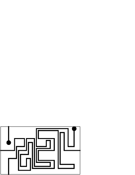
Figure 7: If the variable $\beta$ of the generating functions is real and bigger than the radius of convergence $\beta_{c}$ in infinite volume, the self-avoiding walks start to fill the system and properties depend very much on the boundary conditions. The free extremities of the walks repel one another algebraically.

If one starts with the six vertex model at criticality, then the eight vertex model is the obvious off-critical generalization. In the regime where the elliptic nome is positive, and for $q=e^{i\pi/3}$, the supersymmetry is not spontaneosly broken. (This will be established as a consequence of the results in the next section.) Indeed, it has been known for some time that the singular part of the free energy vanishes for the eight-vertex model for this value of $q$ [41, 48]. In the continnum limit, the eight-vertex model can be thought of as a theory with Landau-Ginzburg potential $W=X^{3}-\lambda X$. In the other regimes, where the theory is non-unitary, we expect that supersymmetry will be broken.

We believe that the foregoing is a generic property of $N=2$ lattice models: there will be an off-critical regime in which supersymmetry is unbroken, and a non-unitary regime where its spontaneously broken.

2.6 Summary

At the end of this long, and perhaps somewhat confusing, section we would like to recall the properties that we expect of an $N=2$ lattice model and summarize them in the form of a strategy that can be used in seeking out such lattice models.

For any Lie algebra, spin and quantum group parameter $q$ there is a natural lattice algebra with which solutions of the Yang-Baxter equations are built. This algebra has several types of representations, including a RSOS one, a vertex one, and some others of mixed type [64]. Choose the value of $q$ such that the RSOS representation is trivial. One obtains then a candidate for a topological sector. Study then the complete model obtained from the vertex representation or maybe the mixed one. Compute in particular its torus partition function and compare it with known $N=2$ ones. To investigate unbroken supersymmetry away from the critical point, study integrable deformations of the critical Boltzmann weights, and (i) check that the free energy has no singular part (ii) compute the scaling dimension and $U(1)$ charge of the lattice operators corresponding to the integrable perturbation and verify that the continuum limit of these operators preserves the supersymmetry.

3 The coset construction of $N=2$ lattice models

Thus far, we have considered only the simplest of the $N=2$ lattice models: those whose qunatum group structure is $U_{q}(SU(2))$ and whose Hilbert space forms a representation of the Temperly-Lieb algebra. The critical, continuum limits of these models are the $N=2$ superconformal minimal models. To go beyond this and obtain theories from models with larger quantum group symmetries, and whose continuum limits are the $N=2$ superconformal coset models, one first finds a formulation of the coset models in which the topological sector has a simple lattice formulation.

Consider the $N=2$ superconformal coset model of the form [66]:

$${\cal M}_{k}(G;H)~{}\equiv~{}{{G_{k}\times SO_{1}(dim(G/H))}\over H}\ ,$$ (24)

where $G$ is simply laced and $G/H$ is a hermitian symmetric space. It was observed in [67] that there is a natural perturbation of this model leading to an $N=2$ supersymmetric quantum integrable field theory, ${\cal M}_{k}^{*}(G;H)$. Moreover, the topological subsector of this quantum integrable model can be identified with the topological coset conformal field theory:

$${{G_{k}\times G_{0}}\over G_{k+0}}\ .$$ (25)

In particular, the correlators of the topological sector of ${\cal M}_{k}^{*}(G;H)$ are all constant, and can be written in terms of the structure constants of the fusion algebra of $G_{k}$. Since lattice analogues of the $G_{k}\times G_{\ell}/G_{k+\ell}$ are well known, the basic approach should now be evident. To see more precisely how the N=2 lattice model is constructed we need to elaborate some of the details of the superconformal model.

3.1 A Coulomb Gas Formulation

For simplicity, take the level of $G$ in (24) to be one (i.e. $k=1$). Let $r$ be the rank of $G$. Since $G$ and $H$ have the same rank, the representations of the current algebra of $G_{1}$ are finitely decomposable as representations of the current algebra of $H_{1}$. Because $G/H$ is a symmetric space, the representations of the current algebra of $SO_{1}(dim(G/H))$ are finitely decomposable into representations of the current algebra of $H_{g-h}$, where $g$ and $h$ are the dual Coxeter numbers of $G$ and $H$ respectively. It follows that ${\cal M}_{k}(G;H)$ can be thought of as a coset model of the form:

$$H_{1}\times H_{g-h}/H_{g-h+1}\ ,$$ (26)

but with a special choice of modular invariant. Because of this equivalence, one can find a Coulomb gas formulation that directly generalizes the $SU(2)$ Coulomb gas formulation of subsection 2.3.2. For $SU(2)$, this was a simple Gaussian model, here one gets a Gaussian model with $r$ free bosons compactified on a scaled version of the weight lattice of $G$. The model has a quantum group symmetry of $U_{q}(H_{0})$ where $H_{0}$ is the semi-simple factor of $H$. (For hermitian symmetric spaces $G/H$, the group $H$ has the form $H=H_{0}\times U(1)$, where $H_{0}$ is semi-simple.) The quantum group parameter, $q$, is the one appropriate to the denominator factor of the coset (26), that is, one takes

$$q~{}=~{}e^{i\pi\over(g-h+1)+h}~{}=~{}e^{i\pi\over g+1}\ .$$ (27)

This choice fixes the radius of comapctification of the Gaussian model to the “supersymmetric radius.”

To reduce the Gaussian model to the requisite coset model one must perform the BRST reduction of the field theory, which, on the lattice, is the quantum group truncation with respect to $U_{q}(H_{0})$. The model knows it origins as ${\cal M}_{k}(G;H)$ essentially because the Gaussian model is compactified upon the scaled weight lattice of $G$. The field theory also contains two operators, ${\cal X}^{+}$ and ${\cal X}^{-}$, that in the Coulomb gas formulation extend the generators of $U_{q}(H_{0})$ to a twisted form of the affine quantum group $U_{q}(\widehat{G})$. In the $N=2$ superconformal model, these operators are hermitian conjugates of each other, they are relevant, and together provide a perturbation that yields a unitary $N=2$ supersymmetric quantum integrable field theory [68, 67]. This is directly parallel to the situation for non-supersymmetric quantum integrable models obtained by conformal perturbation theory: the perturbation is usually one that leads to an affine extension of any underlying quantum group structure. Here, however, one needs two perturbing operators to make the quantum integrable model, one of which extend $U_{q}(H_{0})$ to $U_{q}(G)$ and the other extends this to $U_{q}(\widehat{G})$.

The topological twist of any $N=2$ supersymmetric field theory can be implemented by first replacing the energy momentum tensor by [69, 70]:

$$T^{\rm top}_{\mu\nu}~{}=~{}T^{N=2}_{\mu\nu}~{}+~{}{1\over 2}\epsilon_{\mu\rho}{}~{}g^{\rho\sigma}\partial_{\sigma}J_{\nu}\ ,$$ (28)

where $J_{\nu}$ is the conserved $U(1)$ charge of the $N=2$ supersymmetric theory. With this energy momentum tensor, two of the supercharges become dimension zero charges and can be used as BRST charges to truncate the original Hilbert space down to the topological Hilbert space.

The topological twist shifts the dimension of the operators ${\cal X}^{+}$ and ${\cal X}^{-}$ so that they provide exactly the correct charges to extend $U_{q}(H_{0})$ to $U_{q}(\widehat{G})$. The topological energy mometum tensor thus commutes with $U_{q}(G)$. The type ${\cal I\!I}$ representations of $U_{q}(G)$ at the value of $q$ that we have chosen in (27) are all trivial, and the BRST reduction, or quantum group truncation, will result in a rigid topological model.

In the foregoing discussion we used a minor sleight of hand that we wish to bring into the open. In the continuum field theory formulation of a coset model there are always two quantum groups, one associated with a numerator factor and the other associated with the denominator factor. Thus in (26) there are two quantum groups, the one that we have been discussing with $q$ given by (27), and one associated with the numerator factor of $H_{g-h}$ with $q=e^{i\pi/g}$. Two supercharges can be added to the latter quantum group extending it to a twisted form of $U_{q}(\widehat{G})$, while the extension of the denominator quantum group is accomplished by the relevant perturbing operators ${\cal X}^{+}$ and ${\cal X}^{-}$ as described above. To define the topological theory one is supposed to use one of the supercharges as a BRST charge, and this implicitly suggests that one gets the topological theory using the numerator copy of $U_{q}(G)$. However it should be remembered that the BRST reduction of a Coulomb gas formulation of a coset model can be done using either one of the two quantum groups, and we have used, and will need to use, the denominator copy of the quantum group.

3.2 Formulating the $N=2$ Lattice Models

To build the $N=2$ lattice models one simply reverses the foregoing course. One starts either with a vertex model built using the fundamental representation, ${\cal V}$, of $G$, or with the $IRF$ model whose heights are the weights of $G$. The “topologically twisted” transfer matrix is built from the $\check{R}$-matrix of $U_{q}(G)$. If one performs the quantum group truncation of the vertex model [17, 16], or the restriction of the height model, using the complete $U_{q}(G)$ with $q$ given by (27) the result is a rigid lattice model. In the $IRF$ formulation each successive height will be the unique level one fusion product of the previous height and the representation ${\cal V}$.

To get the $N=2$ lattice model one must topologically untwist the foregoing transfer matrix, breaking the $U_{q}(G)$ symmetry to $U_{q}(H_{0})$ in such a way that the two extra generators in $U_{q}(\widehat{G})$ are given the same spin. One then only performs the quantum group truncation with respect to $U_{q}(H_{0})$, or, in the $IRF$ formulation, only restricts the heights to be affine highest weights of $H_{0}$ at level $g-h+1$, leaving the $U(1)$ direction unrestricted. This is referred to as partial quantum group truncation, or a partial RSOS model. This is the procedure as it was originally implemented in [36]. In [36] the Coulomb gas formulation was extensively analysed to precisely define the topological untwisting of the transfer matrix, and to provide further evidence that the result was indeed an $N=2$ lattice model. In this review we will use more recent results to define the off-critical Boltzmann weights in the $IRF$ formulation of these models with $G=SU(N)$. It turns out that in the off-critical formulation the “untwisting” is easy to describe and is rather intuitive. We begin by reminding the reader about the construction of RSOS models based on the weight lattice of $SU(N)$.

Introduce an orthonormal basis, $f_{j}$, $j=1,\dots,N$, in ${\rm I\kern-1.79993ptR}^{N}$ and define vectors $e_{j}$ by $e_{j}=f_{j}-{1\over N}(f_{1}+\dots+f_{N})$. The vectors $e_{j}$ can be thought of as weights of the fundamental of $SU(N)$. Consider the oriented lattice shown in figure 8. To each vertex assign a height of the form:

$$\Lambda~{}=~{}\Lambda_{0}+\sum_{j=1}^{N-1}~{}n_{j}e_{j}\ ,$$ (29)

where $n_{j}\in{\hbox{\sanse Z\kern-5.03998ptZ}}$ and $\Lambda_{0}$ is an as yet arbitrary vector. This “initial vector,” $\Lambda_{0}$, will play a major role in the forthcoming discussion.

Figure 8: A section of the lattice upon which the model is defined. The bold zig-zag is the initial time slice, and the arrow indicate orientations of edges.

If $\Lambda$ is a height at the beginning of an oriented edge and $\Lambda^{\prime}$ is the height at the other end of the oriented edge, then we require that $\Lambda^{\prime}-\Lambda=e_{j}$, for some $j$. For the typical plaquette shown in figure 9, the evolution is defined by the Boltzmann weights $w(\Lambda,\Lambda+e_{i},\Lambda+e_{j}+e_{j},\Lambda+e_{k}|u)$. Introduce the shorthand notation:

$$[\nu] ~{}\equiv~{} \vartheta_{1}(\gamma\nu|\tau)$$ (30)

$$~{}\equiv~{} 2p^{1\over 8}sin(\pi\gamma\nu)~{}\prod_{n=1}^{\infty}(1-p^{n})(1-e^{2\pi i\gamma\nu}p^{n})(1-e^{-2\pi i\gamma\nu}p^{n})\ ,$$ (31)

where $q=e^{i\pi\gamma}$ is the quantum group parameter and $p\equiv e^{2\pi i\tau}$ is the elliptic nome. Let $\rho$ denote the Weyl vector of $SU(N)$:

$$\rho~{}=~{}{1\over 2}\Big{(}(N-1)e_{1}+(N-3)e_{2}+\dots\dots-(N-1)e_{N}\Big{)}\ .$$ (32)

The non-vanishing Boltzmann weights are as follows [64]:

$$w(\Lambda,\Lambda+e_{i},\Lambda+2e_{i};\Lambda+e_{i}|u) ~{}=~{} {[u+1]\over[1]}$$

$$w(\Lambda,\Lambda+e_{i},\Lambda+e_{i}+e_{j};\Lambda+e_{i}|u) ~{}=~{} {[(\Lambda+\rho)\cdot(e_{i}-e_{j})~{}-~{}u]\over[(\Lambda+\rho)\cdot(e_{i}-e_{j})]}$$

$$w(\Lambda,\Lambda+e_{i},\Lambda+e_{i}+e_{j};\Lambda+e_{j}|u) ~{}=~{}$$

$$\qquad\qquad\qquad\quad{[u]\over[1]}~{}\left({[(\Lambda+\rho)\cdot(e_{i}-e_{j})+1][(\Lambda+\rho)\cdot(e_{i}-e_{j})-1]\over[(\Lambda+\rho)\cdot(e_{i}-e_{j})]^{2}}\right)^{1\over 2}\ ,$$ (33)

where $i\neq j$.

Figure 9: In the IRF formulation the heights, $\Lambda$, are associated to vertices as shown.

To obtain the restricted (RSOS) models corresponding to $G_{\ell}\times G_{1}/G_{\ell+1}$, one takes $\Lambda_{0}=0$, $\gamma=1/(\ell+g+1)$ and restricts the heights to the fundamental affine Weyl chamber of $G_{\ell+1}$. That is, the heights must be affine highest weights of $G_{\ell+1}$. If one were to make this choice of $\Lambda_{0}$ and $\gamma$, but not make this restriction on the heights, then the Boltzmann weights would be singular for certain combinations of heights. It is elementary to verify that the transfer matrix arising from the Boltzmann weights in (33) preserves this restriction. The topological, or rigid model corresponds to setting $\ell=0$.

The lattice analogues [36] of the $N=2$ superconformal grassmannian models:

$${\cal G}_{1,m,n}~{}\equiv~{}{{SU_{1}(m+n)\times SO_{1}(2mn)}\over{SU_{n+1}(m)\times SU_{m+1}(n)\times U(1)}}\ ,$$ (34)

are constructed by once again taking the heights as in (29) (with $N=n+m$). However one now performs the partial restriction by requiring that the heights be affine highest weights of both of the subgroups $SU_{n+1}(m)$ and $SU_{m+1}(n)$ of $SU(m+n)$, but one does not restrict the heights in the $U(1)$ direction. The value of $q$ is taken to be the “topological value” (27). The topological untwisting is accomplished by choosing

$$\Lambda_{0}~{}=~{}{1\over\gamma g}(\rho_{G}-\rho_{H})~{}\tau\ ,$$ (35)

where $\rho_{G}$ and $\rho_{H}$ are the Weyl vectors of $G$ and $H$. For the grassmannian model (34), this is simply

$$\Lambda_{0}~{}=~{}{m+n+1\over 2(m+n)}[n(e_{1}+\dots+e_{m})-m(e_{m+1}+\dots e_{m+n})]\tau\ .$$ (36)

There are several things to note about this choice. First, the proof in [64, 71] that the Boltzmann weights (33) satisfy the star-triangle relations works for a general value of $\Lambda_{0}$ so this model is indeed still exactly solvable. Secondly, $\Lambda_{0}$ is orthogonal to the $SU(m)$ and $SU(n)$ directions and so these sectors of the model behave as if $\Lambda_{0}$ were zero. This means that the transfer matrix preserves the partial restriction on the subgroup $SU(m)\times SU(n)$. Hence this model is an $IRF$ formulation of a particular form of (26). Because the $U(1)$ direction is unrestricted, there is, in principle, a danger that the Boltzmann weights could be singular for some configuartions. In addition, in the physical model, the vector (35) is purely imaginary, and so one might be concerned that the Boltzmann weights may cease to be real in the physical regime. As we will see momentarily the Bolzmann weights are still real and non-singular.

It is convenient to think of the foregoing models from slightly different perspective: the heights can be taken on the partially restricted weight lattice of $G=SU(m+n)$ with $\Lambda_{0}=0$, but the Boltzmann weights must now incorporate the shift (35). We will henceforth adopt this perspective. The shift by $\Lambda_{0}$ does not modify the Boltzmann weights in the $H_{0}=SU(m)\times SU(n)$ direction, but the other Boltzmann weights are, significantly modified. The effect of this shift is to replace certain strategic $\vartheta_{1}$’s by $\vartheta_{4}$’s, and this neatly removes all the potential singularities in the Boltzmann weights owing to the unrestricted $U(1)$. In order to describe the results explicitly let $[\nu]$ be given by (31) and let $\{\nu\}$ is defined by:

$$\{\nu\} ~{}\equiv~{} \vartheta_{4}(\gamma\nu|\tau)$$ (37)

$$~{}\equiv~{} \prod_{p=1}^{\infty}(1-p^{n})(1-e^{2\pi i\gamma\nu}p^{n-{1\over 2}})~{}(1-e^{-2\pi i\gamma\nu}p^{n-{1\over 2}})\ .$$ (38)

Set the parameter $\gamma$ to ${1\over m+n+1}$, and take the vector $\Lambda_{0}$ to be zero. The non-vanishing Boltzmann weights are then as follows:

If $1\leq i,j\leq m$ or $m+1\leq i,j\leq m+n$ then, for $i\neq j$, one has:

$$w(\Lambda,\Lambda+e_{i},\Lambda+2e_{i};\Lambda+e_{i}|u) ~{}=~{} {[u+1]\over[1]}$$

$$w(\Lambda,\Lambda+e_{i},\Lambda+e_{i}+e_{j};\Lambda+e_{i}|u) ~{}=~{} {[(\Lambda+\rho)\cdot(e_{i}-e_{j})~{}-~{}u]\over[(\Lambda+\rho)\cdot(e_{i}-e_{j})]}$$

$$w(\Lambda,\Lambda+e_{i},\Lambda+e_{i}+e_{j};\Lambda+e_{j}|u) ~{}=~{}$$

$$\qquad\qquad\qquad\quad{[u]\over[1]}~{}\left({[(\Lambda+\rho)\cdot(e_{i}-e_{j})+1][(\Lambda+\rho)\cdot(e_{i}-e_{j})-1]\over[(\Lambda+\rho)\cdot(e_{i}-e_{j})]^{2}}\right)^{1\over 2}\ .$$ (39)

If $1\leq i\leq m$ or $m+1\leq j\leq m+n$, or vice-versa, then one has

$$w(\Lambda,\Lambda+e_{i},\Lambda+e_{i}+e_{j};\Lambda+e_{i}|u) ~{}=~{} {\{(\Lambda+\rho)\cdot(e_{i}-e_{j})~{}-~{}u\}\over\{(\Lambda+\rho)\cdot(e_{i}-e_{j})\}}$$

$$w(\Lambda,\Lambda+e_{i},\Lambda+e_{i}+e_{j};\Lambda+e_{j}|u) ~{}=~{}$$

$$\qquad\qquad\qquad\quad{[u]\over[1]}~{}\left({\{(\Lambda+\rho)\cdot(e_{i}-e_{j})+1\}\{(\Lambda+\rho)\cdot(e_{i}-e_{j})-1\}\over\{(\Lambda+\rho)\cdot(e_{i}-e_{j})\}^{2}}\right)^{1\over 2}\ .$$ (40)

From the Coulomb gas analysis of [36] and as confirmed by the Bethe Ansatz computations in [37], the foregoing height model at criticality yields the Neveu-Schwarz sector of the $N=2$ superconformal model. The Ramond sector can be obtained by a uniform spectral flow in the $U(1)$ direction. This is easily implemented: one shifts all the lattice height appropriately, or equivalently one takes $\tau\to\tau+1$ in (35).

3.3 Some simple properties of these models

As has already been mentionned, a signal that a model is supersymmetric is that the free energy per lattice site is analytic when the supersymmetry is unbroken. For the models discussed in the last subsection, this computation is very revealing in that it also exhibits and utilizes the connection between the supersymmetric model and its topological sector. We will begin, however, by illustrating the foregoing construction for $G=SU(2)$, and relate it to the constructions of section 2.

3.3.1 A simple example

For $G=SU(2)$ the foregoing lattice model construction collapses to what is basically the $IRF$ version of the eight-vertex model [41, 48]. The weight vectors $e_{1}$ and $e_{2}$ of the foregoing subsection satisfy $e_{1}=-e_{2}$, and the Weyl vector is given by $\rho=e_{1}$. The unrestricted heights lie on the weight lattice of $SU(2)$, which we will parametrize by an integer, $\ell$, where $\Lambda=\Lambda_{0}+(\ell-1)e_{1}$. The integer, $(\ell-1)$, is equal to twice the spin of the corresponding $SU(2)$ weight. These are exactly the heights discussed in section 2.3.1. If one takes $\Lambda_{0}=0$ and $\gamma=1/3$ then the quantum group truncated model is completely rigid with $\ell$ alternating between $1$ and $2$. There are thus two states in this model depending upon whether a given site has height $1$ or $2$. This is the $SU_{1}(2)/SU_{1}(2)$ lattice model. To get the lattice analogue of the $N=2$ supersymmetric theory, one should only quantum group truncate with respect to the $H$ subgroup, or more precisely, with respect to the semi-simple part, $H_{0}$, of $H$. In this instance, this means that one performs no quantum group truncation at all, and one therefore has a Gaussian model. The height, $\ell$, takes the values $0,1$ or $2$ modulo $3$, and values of $\gamma$ and $\Lambda_{0}$ are:

$$\gamma~{}=~{}{1\over 3}\qquad{\rm and}\qquad\Lambda_{0}~{}=~{}{3\over 2}~{}e_{1}~{}\tau\ .$$ (41)

We have thus “unfrozen” the heights $\ell$ of the RSOS model and have avoided the problem of singular Boltzmann weights through the choice of $\Lambda_{0}$. As described in section 2.3.2, this value of $\gamma$ means that at criticality and in the continuum the Gaussian model is the $N=2$ superconformal minimal model, with central charge, $c=1$. The off-critical $N=2$ supersymmetic, quantum integrable model corresponds to the most relevant chiral primary perturbation of the conformal model [11], and may be thought of as sine-Gordon at the supersymmetric value of the coupling constant. From (39) and (40) the elliptic Boltzmann weights are the following:

$$w(\ell,\ell\pm 1,\ell\pm 2;\ell\pm 1|u) = {\vartheta_{1}({1\over 3}(u+1)|\tau)\over\vartheta_{1}({1\over 3}|\tau)}\qquad\qquad\qquad$$

$$w(\ell,\ell\pm 1,\ell;\ell\pm 1|u) = {\vartheta_{4}({1\over 3}(\ell\mp u)|\tau)\over\vartheta_{4}({\ell\over 3}|\tau)}\qquad\qquad\qquad$$

$$w(\ell,\ell\pm 1,\ell;\ell\mp 1|u) = {\vartheta_{1}({u\over 3}|\tau)\over\vartheta_{1}({1\over 3}|\tau)}\left({{\vartheta_{4}({1\over 3}(\ell-1)|\tau)~{}\vartheta_{4}({1\over 3}(\ell+1)|\tau)}\over(\vartheta_{4}({\ell\over 3}|\tau))^{2}}\right)^{1\over 2}\ .$$

These Boltzmann weights are precisely the same as those of the $A_{2}^{(1)}$ cyclic solid-on-solid models described in [41, 49]. In this context the labelling of the model by $A_{2}^{(1)}$ refers to the fact that, because of the periodicity of the Boltzmann weights, the unrestricted $U(1)$ is, in fact, cyclic and so rather than taking the heights to be in ZZ one can view them as living on the extended Dynkin diagram of $A_{2}$.

3.3.2 The free energy

The easiest way to compute the free energy per unit volume, ${\cal F}$, is to use its analytic and inversion properties (see chapter 13 of [41]). In this review we will only consider regime $I\!I\!I$ of the $SU(N)$ model, i.e. $0<p\equiv e^{2\pi i\tau}<1$, $-{1\over 2}N<Re(u)<0$. (This regime corresponds to the unitary, quantum integrable field theory of interest – other regimes either have different conformal limits or correspond to perturbations with imaginary coupling.) We will also consider the models defined by (38) – (40) where $\gamma$ is now an arbitrary, positive, real parameter.

To compute ${\cal F}$ it is first convenient to multiply the Boltzmann weights (38) – (40) by a factor of

$$e^{{i\pi\gamma^{2}\over\tau}(u^{2}+{2u\over N})}\ ,$$ (42)

and perform the modular inversion $\tau\to-1/\tau$. After making a gauge transformation one then finds that the Boltzmann weights are manifestly periodic under:

$$u~{}\to~{}u~{}+~{}{2\tau\over\gamma}\ .$$ (43)

One then writes

$${\cal F}~{}=~{}-\ log(\kappa(u))\ ,$$

and requires that $log(\kappa)$ be analytic in a region containing regime $I\!I\!I$ and also be periodic under (43). Note that one does not impose the other periodicity of the theta functions ($u\to u+{2\over\gamma}$) because such shifts of $u$ would go outside the domain of analyticity of the free energy.

Using the properties of the corner transfer matrix one can show that $\kappa(u)$ must also satisfy:

$$\kappa(u)~{}\kappa(-u)~{}=~{}h(1-u)~{}h(1+u)\ ,$$ (44)

$$\kappa(\lambda+u)~{}\kappa(\lambda-u)~{}=~{}h(\lambda-u){}~{}h(\lambda+u)\ ,$$ (45)

where $\lambda=-N/2$ for $SU(N)$, and

$$h(u)~{}\equiv~{}{\vartheta_{1}({u\gamma\over\tau}|{-{1\over\tau}})\over\vartheta_{1}({\gamma\over\tau}|{-{1\over\tau}})}\ .$$ (46)

The function $h(u)$ that appears on the right hand side of these equations depends only upon the inversion relations of the elliptic Boltzmann weights. These equations, along with analyticity and periodicity, determine $log(\kappa(u))$ completely. One simply writes $log(\kappa(u))$ as a general Fourier series in $e^{i\pi\gamma u/\tau}$ and uses (44) and (45) to determine the coefficients. This is a little tedious but it is straightforward.

At this point one should note that the foregoing equations and constraints do not depend on the choice of $\Lambda_{0}$. This means that the free energy for all of of the lattice analogues of the grassmannian models (34) only depends upon $N=m+n$, and this free energy is exactly that of the topological $SU_{1}(N)\times SU_{0}(N)/SU_{1}(N)$ model. This will be a general feature of these models, the free energy of the models will be equal to that of the rigid topological model, and thus it must be possible to normalize the elliptic Boltzmann weights analytically so that the free energy is zero.

The fact that the free energy is independent of $\Lambda_{0}$ also means that we can use the known results for $\Lambda_{0}=0$ for the models based on $SU(N)$ [72]. One therefore has

$$log(\kappa(u))~{}=~{}log\left({\vartheta_{1}(\gamma(u+1)|\tau)\over\vartheta_{1}(\gamma|\tau)}\right)~{}-~{}\sum_{k=-\infty}^{k=\infty}~{}f(k;u,\gamma,\tau)\ ,$$ (47)

where

$$f(x;u,\gamma,\tau)~{}\equiv~{}{{sinh\big{(}{\pi i\over\tau}(1-\gamma)x\big{)}~{}sinh\big{(}{2\pi i\over\tau}\gamma ux\big{)}~{}sinh\big{(}{\pi i(N-1)\over\tau}\gamma x\big{)}}\over{x~{}sinh\big{(}{\pi i\over\tau}x\big{)}~{}sinh\big{(}{\pi iN\over\tau}\gamma x\big{)}}}\ .$$ (48)

This expression differs slightly from that of [72] in that we have subtracted the logarithm of the phase (42) so that the result is no longer exactly periodic under (43), but so that it does give the free energy for the model defined by the Boltzmann weights in (39) and (40).

To obtain the result as a function of $p=e^{2\pi i\tau}$ one needs to perform the modular inversion of the second term in (47). This can be done by Poisson resummation (see, for example, chapter 10 of [41], or appendix D of [73]). That is, one defines

$$\hat{f}(\zeta)~{}\equiv~{}\int_{-\infty}^{+\infty}~{}e^{2\pi i\zeta x}~{}f(x)~{}dx$$ (49)

and uses the equality:

$$\sum_{k=-\infty}^{k=\infty}~{}f(k)~{}=~{}\sum_{k=-\infty}^{k=\infty}~{}\hat{f}(k)\ .$$ (50)

The fourier transform of (48) can be performed by closing the contour above or below the real axis, depending upon the sign of $\zeta$, and then summing the residues. This sum over residues and the sum in (47) generates an expansion in powers of $p$. The vanishing of $sinh({\pi iN\over\tau}\gamma x)$ in denominator of (47) gives rise to residues that are proportional to $p^{1\over N\gamma}$. This is the source of the non-analytic behaviour of the free energy as a function of $p$. The residues coming from the vanishing of the other $sinh$ function in the denominator of (47) are all proportional to integral powers of $p$. It is easy to extract the leading behaviour as $\tau\to i\infty$ from this sum over residues. One finds

$${\cal F}~{}\sim~{}{{4~{}sin\big{(}{1\over N}\big{(}{1\over\gamma}-1\big{)}\pi\big{)}~{}sin\big{(}{2\pi u\over N}\big{)}~{}sin\big{(}{\pi\over N}\big{)}}\over{sin\big{(}{\pi\over N\gamma})}}~{}~{}p^{1\over N\gamma}\ .$$ (51)

For generic values of $\gamma$ this means that ${\cal F}\sim p^{1\over N\gamma}$, while from hyperscaling one has ${\cal F}\sim{1\over\xi^{2}}$, where $\xi$ is the correlation length. Therefore, we have

$$\tau~{}\sim~{}{iN\gamma\over\pi}~{}log(\xi)\ ,$$ (52)

as $\tau\to i\infty$.

One should note that for

$$\gamma^{-1}~{}=~{}Nj~{}+~{}1,\qquad j=1,2,3,\dots$$ (53)

the numerator of (48) vanishes whenever $sinh({\pi iN\over\tau}\gamma x)$ vanishes. As a result, the Poisson resummation of (47) gives rise to an expansion in integral powers of $p$. That is, if $\gamma$ satisfies (53) then the free energy is an analytic function of $p$. The choice $\gamma^{-1}=N+1$ corresponds to our supersymmetric models.

For these special values of $\gamma$ it is, of course, no longer true that ${\cal F}\sim p^{1\over N\gamma}$ as $\tau\to i\infty$. However, continuity in $\gamma$ means that the relation (52) is true even at these special values.

It turns out that for $\gamma$ given by (53) one can easily express the free energy in terms of theta functions. Here we will give the result for the supersymmetric model: $\gamma^{-1}=N+1$. The general case is similar. For $\gamma=1/(N+1)$, the second term in (47) can be written:

$${2\pi i\over\tau}~{}u\gamma(1-2\gamma)~{}-~{}\sum_{k=1}^{\infty}~{}{1\over k(1-\tilde{p}^{k})}~{}(z^{k}-z^{-k})~{}(w^{-k}-w^{-kN})\ ,$$ (54)

where $\tilde{p}=e^{-2\pi i/\tau}$, $z=e^{2\pi i\gamma u/\tau}$ and $w=e^{2\pi i\gamma/\tau}$. This is a standard expansion of the logarithm of the ratio of two theta functions. Finally one can perform modular inversions on the theta functions and the final result is

$$log(\kappa(u))~{}=~{}log\left({\vartheta_{1}(\gamma(u-1)|\tau)\over\vartheta_{1}(\gamma|\tau)}\right)~{}=~{}log\left({[u-1]\over[1]}\right)\ .$$ (55)

Observe that, as promised, this free energy is analytic in the whole of regime $I\!I\!I$. Indeed, if one multiplies all of the Boltzmann weights in (39) and (40) by ${[1]\over[u-1]}$ then the Boltzmann weights are still analytic in regime $I\!I\!I$, and the free energy, ${\cal F}$, vanishes identically.

3.3.3 The off-critical perturbing operators

For the critical limit of these models one can use Coulomb gas methods to show that the continuum limit is $N=2$ supersymmetric. The free energy computations suggest that the off-critical models are also $N=2$ supersymmetric in the continuum, but we would like to demonstrate this more directly.

From the analysis of the perturbations of $N=2$ superconformal coset models, we know that the are natural perturbations that lead to $N=2$ supersymmetric quantum integrable models. These operators have the form:

$$\psi~{}\equiv~{}G_{-{1\over 2}}^{-}\widetilde{G}_{-{1\over 2}}^{-}\phi\qquad{\rm and}\qquad\tilde{\psi}~{}\equiv~{}G_{-{1\over 2}}^{+}\widetilde{G}_{-{1\over 2}}^{+}\tilde{\phi}\ ,$$ (56)

where $\phi$ is a very particular chiral primary field, and $\tilde{\phi}$ is its anti-chiral conjugate. In particular, the fields $\psi$ and $\tilde{\psi}$ have conformal weights and $U(1)$ quantum numbers:

$$h_{\psi}~{}=~{}\bar{h}_{\psi}~{}=~{}h_{\tilde{\psi}}~{}=~{}\bar{h}_{\tilde{\psi}} ~{}=~{} {1\over 2}~{}+~{}{1\over 2(N+1)}$$

$$Q_{\psi}~{}=~{}\bar{Q}_{\psi}~{}=~{}-Q_{\tilde{\psi}}~{}=~{}-\bar{Q}_{\tilde{\psi}} ~{}=~{} 1~{}-~{}{1\over(N+1)}$$ (57)

We remarked above that in the vertex form of the model at criticality, these operators extend $U_{q}(H_{0})$ to $U_{q}(G)$. Thus, based on general expectations about lattice models, one would expect these operators to be the ones that correspond to the elliptic “deformation” of the critical model. We can see this connection much more explicitly as follows.

Consider the continuous family of models where the initial height vector is taken to be

$$\Lambda_{0}~{}=~{}{2\mu\over\gamma g}(\rho_{G}-\rho_{H})~{}\tau\ ,$$ (58)

where $\mu$ is a parameter. When $\mu=0$ we have the topological model and the lowest powers of $p$ in the Boltzmann weights (33) are $p^{0}$ and $p^{1}$. If we increase $\mu$, then the lowest powers of $p$ change smoothly to $p^{\mu}$ and $p^{(1-\mu)}$. Now recall that in the scaling limit, $\tau\to i\infty$, we know that $\tau$ is related to the correlation length by (52), and thus $p\sim\xi^{-{2N\over N+1}}$. It follows that the elliptic perturbation must involve two operators, and that their coupling constants must scale as $p^{\mu}\sim\xi^{-{2N\mu\over N+1}}$ and $p^{(1-\mu)}\sim\xi^{-{2N(1-\mu)\over N+1}}$. The corresponding operators therefore have conformal weights:

$$h_{1}~{}=~{}\bar{h}_{1}~{}=~{}1~{}-~{}{N\mu\over(N+1)}\ ;\quad\quad h_{2}~{}=~{}\bar{h}_{2}~{}=~{}1~{}-~{}{N(1-\mu)\over(N+1)}\ .$$ (59)

When $\mu={1\over 2}$ these two operators have precisely the same conformal dimension and this is the conformal dimension given in (57). If we now consider the gradual untwisting of the energy momentum tensor of the quantum field theory:

$$T(z)~{}=~{}T^{\rm top}(z)~{}-~{}\mu~{}\partial J(z)\ ;\quad\quad\widetilde{T}(\bar{z})~{}=~{}\widetilde{T}^{\rm top}(\bar{z})~{}+~{}\mu~{}\bar{\partial}\widetilde{J}(\bar{z})\ ,$$ (60)

we see that the conformal weights of the operators (56) depend upon the parameter $\mu$ exactly as in (59).

In this way one can not only identify the dimensions of the perturbations that lead to the elliptic Boltzmann weights, but one can also determine their $U(1)$ charges. Moreover, the foregoing also demonstrates that smoothly changing the initial lattice vector, $\Lambda_{0}$, causes the dimensions of the perturbing operators to change in exactly the way that they should under topological untwisting. As a result one also obtains further confirmation that one has correctly determined the lattice analogue of topological untwisting. A more explicit relation between $\Lambda_{0}$ and perturbed conformal theories can be obtained using the method of [59].

4 Scattering matrices

Since we are considering critical and off-critical $N=2$ lattice models, there will of course be massless and massive $S$-matrices associated with the excitations of these models. There have been quite a number of papers written on this subject (see, for example, [11, 50, 12, 13, 51, 52, 53]), and we will not try perform even a partial survey. Our purpose here is to simply make a few remarks about some of the known $S$-matrices, and how their construction fits in with the general strategy of the construction of $N=2$ lattice models.

It is first useful to recall some general observations about conformal coset models and their perturbations leading to quantum integrable models. In a generalized Coulomb gas description of the conformal model, there are always two quantum groups that usually have the same underlying Lie algebra, but have different roots of unity. One of these quantum groups is generically associated with the numerator of the coset, while the other quantum group is associated with the denominator. The corresponding lattice model only exhibits one of these quantum group symmetries, and it is usually the one associated with the denominator of the coset model. The perturbing operators that lead to quantum integrable models usually extend this lattice (or denominator) quantum group to a larger, affine quantum group. The other (numerator) quantum group usually plays a major role in the scattering theory of the quantum integrable model. That is, the scattering matrices are usually built out of the $\check{R}$-matrices of this numerator quantum group. The corresponding affine extension of the scattering quantum group leads to operators in the theory that commute with the $S$-matrix. Such non-local conserved charges have been used extensively in the construction of the $S$-matrices. The intuitive reason as to why the scattering theory and lattice quantum groups are distinct is that the solitons of the scattering theory must be local with respect to the perturbing operators leading to the quantum integrable model [54].

The supersymmetric models also fit this mould. The denominator quantum group is indeed that of the lattice model, while numerator quantum group is that of the scattering theory. The non-local conserved charges that extend the scattering quantum group to the affine quantum group are simply the supersymmetry generators. Thus we find that while almost all of our lattice models do not have explicit supersymmetry, the corresponding scattering theories do. In other words supersymmetry appears only as a dynamical symmetry.

4.1 Massless $S$-matrices and the six-vertex model

The six-vertex model is diagonalizable by Bethe ansatz [41], and the solutions are classified in terms of $1,2$ strings and the anti-string $1^{-}$, with a coupling diagram as in figure 10 (see [57]). To study the scattering theory simply observe that for a relativistic QFT the thermodynamic Bethe ansatz [58], in addition to the pseudo-particles appearing in the solution of the Bethe equations, involves an additional physical particle, as in figure 10.

Figure 10: The first diagram represents the pseudo-particles (solutions of the Bethe ansatz) and their couplings at the supersymmetric point of the lattice vertex model. Recall that for $q=e^{i\pi/t}$ one has strings $(1,2,\ldots,t-1)$ and the anti-string $a$. In the continuum theory there is an additional node for the physical particles, indicated by a heavy dot on the second diagram. Therefore the number of Bethe ansatz solutions must differ by one from the lattice case, hence the denominator of the quantum group parameter must also differ by one from the lattice case.

Therefore, if the lattice model has $q=\exp(i\pi/3)$, the scattering theory has $q^{\prime}=\exp(i\pi/2)$. From the lattice model, a massless scattering theory [60] can be extracted which has the following content (see [59, 61]). One has a pair of right moving particles which we parametrize as

$$e_{R}=p_{R}={M\over 2}e^{\theta}$$ (61)

and a pair of left moving particles with

$$e_{L}=-p_{L}={M\over 2}e^{-\theta}$$ (62)

where $M$ is a mass scale and $\theta$ is a rapidity. These particles have fermion number equal to $\pm 1$ and they have factorized scattering with

$$S_{LL}=S_{RR}=Z(\theta)\left(\begin{array}[]{cccc}\cosh\theta/2&0&0&0\\ 0&i\sinh\theta/2&1&0\\ 0&1&i\sinh\theta/2&0\\ 0&0&0&\cosh\theta/2\end{array}\right)$$ (63)

where $Z(\theta)$ is a normalization factor ensuring unitarity and crossing symmetry, while the LR scattering is trivial

$$S_{LR}=S_{RL}=1$$ (64)

Acting on the right particles $u,d$ we have

$$Q_{-}|u(\theta)>=\sqrt{M/2}e^{\theta/2}|d(\theta)>$$ (65)

$$Q_{+}|d(\theta)>=\sqrt{M/2}e^{\theta/2}|u(\theta)>$$ (66)

and same type of relations with left particles and $\bar{Q}^{\pm}$ generators. The supersymmetry algebra is

$$Q_{+}^{2}=Q_{-}^{2}=\bar{Q}_{+}^{2}=\bar{Q}_{-}^{2}=\{Q_{+},\bar{Q}_{-}\}=\{Q_{-},\bar{Q}_{+}\}=0$$ (67)

$$\{Q_{+},\bar{Q}_{+}\}=\{Q_{-},\bar{Q}_{-}\}=0$$ (68)

$$\{Q_{+},Q_{-}\}=Me^{\theta},\ \{\bar{Q}_{+},\bar{Q}_{-}\}=2Me^{-\theta}$$ (69)

4.2 Massive $S$-matrices

There are several ways in which one can extract the $S$-matrices of the massive quantum integrable models that appear in the continuum limits of the $N=2$ lattice models. We will briefly discuss two of them here. The first approach is that taken in [11, 12], and the starting point is to use the Landau-Ginzburg description of the model to determine the ground-state and soliton structure. Since the solitons are generically doublets of the superalgebra, one can then use the Bogomolnyi bounds in the superalgebra to determine the soliton masses. The solitons also have fractional fermion numbers that can be determined from the Landau-Ginzburg potential. This information, combined with the fact that the $S$-matrix must commute with the supersymmetry, be unitary, satisfy the Yang-Baxter equations, and obey crossing symmetry is more than enough to determine the $S$-matrix completely. This has been done for a large class of models [12], but there is an even larger class for $N=2$ quantum integrable models for which the $S$-matrices are not known. The first reason for this is that one can easily show that in this larger class the solitons alone cannot form a kinematically closed scattering theory [11, 51]. This almost certainly means that breather states must be included in the spectrum. This does not pose, a priori, any obstacle to the construction of the $S$-matrices, but as we will describe below, there could be some further conceptual problems to be solved if one is to determine the $S$-matrices for these more general models.

We will describe the second method of obtaining the $S$-matrices in more detail here since it is rather more in the spirit of our approach to $N=2$ lattice models. The basic idea is to once again use topological models and a modification of quantum group truncation.

The scattering matrices are well known for the quantum integrable models obtained from the natural perturbations of the $G_{k}\times G_{\ell}/G_{k+\ell}$ coset models (see, for example, [74, 75, 76, 77, 78, 79, 80]). For simplicity we will only consider the models with with $G=SU(N)$ and the level $k$ equal to one. The $S$-matrices can then be obtained from RSOS restrictions of affine Toda $S$-matrices. Let $W_{j}$, $j=1,\dots,N-1$, denote the fundamental representations of $SU(N)$ (i.e. the anti-symmetric tensors of rank $j$). Each of these representations defines a multiplet of solitons of affine $\widehat{SU(N)}$-Toda, and these solitons can be labelled by the weights of the representations.

Define $S^{(\widehat{G})}_{ji}(\theta,q)$ to be the two-body $S$-matrix for the scattering of particles in $W_{i}$ with those in $W_{j}$:

$$S^{(\widehat{G})}_{ji}(\theta,q):\quad W_{i}\otimes W_{j}~{}\to~{}W_{j}\otimes W_{i}\ ,$$ (70)

where, as usual, $\theta$ is the relative rapidity of the solitons and $q$ is the quantum group parameter. Requiring the $S$-matrix to commute with the $U_{q}(\widehat{SU(N)})$ symmetry leads to the following result:

$$S^{(\widehat{G})}_{ji}(\theta,q)~{}=~{}X_{ji}(\theta)\ v_{ji}(\theta,q)\ R_{ji}(\theta,q)\ .$$ (71)

The last term, $R_{ji}(\theta,q)$, is the standard $R$-matrix for the quantum group $U_{q}(\widehat{SU(N)})$ in the principal gradation. The spectral parameter, $x$, and the quantum group parameter, $q$, of the $R$-matrix are related to the rapidity, $\theta$ and the Toda couping constant, $\beta$, by:

$$q~{}=~{}exp\left(-{i\pi\over\beta^{2}}\right)\ ,\quad x~{}=~{}exp\left({\theta\over\gamma}\right)\qquad{\rm where}\qquad\gamma~{}=~{}{\beta^{2}\over 1-\beta^{2}}\ .$$ (72)

The scalar factor, $v_{ji}(\theta,q)$, in (71) is the minimal factor that makes the product $v_{ji}R_{ji}$ crossing symmetric and unitary. This is relatively easy to compute and can be found in [75, 76]. The additional scalar factor $X_{ji}(\theta)$ is a CDD factor, and it satisfies crossing and unitarity by itself. This factor contains all of the necessary poles for closure of the bootstrap with the spectrum of soliton masses. It turns out that this CDD factor does not depend upon the value of the Toda coupling and so can be evaluated by going to the limit ($\beta\to 1$) in which the Toda model can be related to a Gross-Neveu model [75].

To get the model corresponding to the perturbed coset model one must first incorporate the background charge, which is done in an analogous manner to the twist in the Markov trace of subsection 2.3.4. Let $H$ be some subgroup of $G=SU(N)$, where $H$ also has rank $N-1$, and let $\rho_{H}$ be the Weyl vector of $H$. Define $S^{({\widehat{G}}/H)}_{ji}(\theta,q)$ by

$$S^{({\widehat{G}}/H)}_{ji}(\theta,q)~{}=~{}\left(x^{-\rho_{H}\cdot h}\otimes x^{-\rho_{H}\cdot h}\right)~{}S^{({\widehat{G}})}_{ji}~{}\left(x^{\rho_{H}\cdot h}\otimes x^{\rho_{H}\cdot h}\right)\ ,$$ (73)

where $h$ represents the vector of Cartan subalgebra generators of the quantum group. This conjugation only affects the $R$-matrix part of the $S$-matrix, and for $H=G$, it converts the principal gradation to the homogeneous gradation.

By construction, the S-matrices $S^{({\widehat{G}}/H)}_{ji}(\theta,q)$ commute with the action of the finite quantum group $U_{q}(H)$. These generators act in the more familiar rapidity independent fashion. Therefore one can use the $U_{q}(H)$ symmetry to restrict the model exactly as in the lattice model.

For each weight, $\mu$, of $W_{j}$ we introduce a formal operator $K^{(j)}_{\mu}(\theta)$. These operators satisfy an $S$-matrix exchange relation:

$$K^{(j)}_{\mu}(\theta_{1})\ K^{(i)}_{\nu}(\theta_{2}){}~{}=~{}\sum_{\mu^{\prime},\nu^{\prime}}\left(S^{({\widehat{G}}/H)}_{ji}(\theta,q)\right)^{\mu^{\prime},\nu^{\prime}}_{\mu,\nu}~{}K^{(i)}_{\nu^{\prime}}(\theta_{2})\ K^{(j)}_{\mu^{\prime}}(\theta_{1})\ .$$

Let ${\cal F}$ denote the multi-particle fock space generated by the formal action of the operators $K^{(j)}_{\mu}(\theta)$ on the vacuum. The space ${\cal F}$ is an $U_{q}(H)$ module, and reducible (for $q$ not a root of unity):

$${\cal F}=\bigoplus_{a}~{}V^{(\lambda^{(H)}_{a})}\ ,$$

where $V^{(\lambda^{(H)}_{a})}$ is an $U_{q}(H)$ module of highest weight $\lambda^{(H)}_{a}$. Since the $K^{(j)}_{\mu}(\theta)$ act on ${\cal F}$, one can consider their reduction

$$K^{(n)}_{\lambda^{(H)}_{b}\lambda^{(H)}_{a}}(\theta):\quad V^{(\lambda^{(H)}_{a})}\longrightarrow V^{(\lambda^{(H)}_{b})}.$$

These operators satisfy the exchange relation:

$$K^{(j)}_{\lambda^{(H)}_{b}\lambda^{(H)}_{a}}(\theta_{1})\ K^{(i)}_{\lambda^{(H)}_{a}\lambda^{(H)}_{c}}(\theta_{2})\ {}~{}=~{}\qquad\qquad\qquad\qquad\qquad\qquad\qquad\qquad\qquad$$

$$\qquad\qquad\qquad\qquad\sum_{\lambda^{(H)}_{d}}\left(S^{({\widehat{G}}/H)}_{ji}(\theta,q)\right)^{\lambda^{(H)}_{b}\lambda^{(H)}_{d}}_{\lambda^{(H)}_{a}\lambda^{(H)}_{c}}~{}K^{(i)}_{\lambda^{(H)}_{b}\lambda^{(H)}_{d}}(\theta_{2})\ K^{(j)}_{\lambda^{(H)}_{d}\lambda^{(H)}_{c}}(\theta_{1})\ .$$

The S-matrix for the kinks in this equation is the SOS form, and the foregoing construction is once again the vertex/SOS correspondence.

As before, the restriction amounts to taking $q$ to be a root of unity and imposing a limitation on the allowed highest weight labels $\lambda^{(H)}$. To get the $S$-matrix for the preturbed coset model $G_{1}\times H_{\ell}/H_{\ell+1}$ one must take the Toda coupling so that $\beta^{2}=(\ell+h)/(\ell+h+1)$, where $h$ is the dual Coxeter number of $H$. Therefore, one has:

$$q~{}=~{}-exp(-i\pi/(\ell+h))\ .$$ (74)

Note that this is the root of unity appropriate to the quantum group structure of the numerator quantum group of the coset model.

To get the $N=2$ supersymmetric models one chooses $H$ so that $G/H$ is hermitian symmetric, and takes $\ell=g-h$. Thus one has $q=-e^{-i\pi/g}$. If one were to take $H=G$ one would once again get the topological coset model, but with the foregoing choice of $q$, the only $U_{q}(G)$ representation with non-vanishing $q$-dimension is the singlet representation. There are thus no solitons in the topological model. Once again one finds the $N=2$ model by modifying the quantum group truncation procedure. One can also verify that under the twisting process (73), the two generators that extend $U_{q}(H)$ to $U_{q}(\widehat{G})$ have a rapidity dependence that makes them spin-${1\over 2}$ charges. If the quantum group truncation procedure parallels that of the conformal theory, then these operators will become the supersymmetry generators of the restricted model.

This process works beautifully and simply for $G=SU(N)$ and $H=SU(N-1)\times U(1)$. For this choice, the fundamental reprexentations $W_{j}$ decompose into a direct sum of two representations of $U_{q}(SU(N-1))$. In the RSOS truncation using $U_{q}(H)$ one therefore finds that each $W_{j}$ yields two solitons, and these form a supersymmetric doublet. The $U(1)$ charge becomes the (fractional) fermion number, and the two generators that extend $U_{q}(H)$ to $U_{q}(\widehat{G})$ act as the supersymmetry on this doublet. We have thus incorporated the supersymmetry directly into the affine quantum group. The $S$-matrices for the $N=2$ model can then be easily extracted from the Toda $S$-matrices for $G=SU(N)$ [13].

The surprise comes once one tries this procedure for more general models of the form (34), for example, for $G=SU(4)$, $H=SU(2)\times SU(2)\times U(1)$. The problem is that the quantum group truncation does not respect canonical supermultiplet structure. In these more general models all of the $W_{j}$’s give rise to RSOS solitons with fractional fermion numbers that agree with the Landau-Ginzburg picture. All of the RSOS solitons coming from one of the $W_{j}$’s are, of course, transformed into each other by the generators of $U_{q}(\widehat{G})$. The two generators that extend $U_{q}(H)$ to $U_{q}(\widehat{G})$ are indeed spin-${1\over 2}$ and commute with the $S$-matrix. The problem is that there does not seem to be an RSOS truncation upon which the algebra of these generators becomes that of the standard $N=2$ superalgebra. For example, some $W_{j}$’s would give rise to a three dimensional “supermultiplet.” (This happens in the $SU(4)$ example above for the six-dimensional representation of $SU(4)$.)

There are several possible resolutions of this issue. It is quite conceivable that the Toda approach breaks down, or it might be that there is some supersymmetry anomaly. It is also possible that the integrable model gives rise to two $S$-matrices, one in which the supersymmetry acts locally, and one in which it does not. It is certainly of interest to resolve this problem. As first sight, the possibility of a supersymmetry anomaly seems the least likely explanation. However, such an explanation is

perhaps not quite as outrageous as it sounds, after all, the supersymmetry would still be a symmetry of the $S$-matrix, but it would simply have non-trivial braiding relations with single soliton states. Such a phenomenon is already present in the models that we do understand: the fractional fermion number of single solitons means that the supersymmetry action on single solitons must involve extra phases. It is just conceivable that the more exotic models exhibit a more involved (perhaps non-abelian) form of this. At any rate, it is highly desirable to compute the $S$-matrices for these models. It is also, perhaps, significant that these “exotic” models are also precisely the ones for which the $S$-matrices are not yet known because the solitons cannot, by themselves, form a closed scattering theory.

5 Other issues

5.1 Spontaneous breaking of $N=2$ supersymmetry

In lattice models there is a natural direction of perturbation that does not break supersymmetry explicitly, but does so spontaneously. This is made possible by the non-unitarity of the perturbation. For example, consider the polymer problem discussed earlier. The critical Landau-Ginzburg potential in this theory is $W=X^{3}$, and the perturbation that changes the weight $\beta$ of monomers in the generating functions corresponds exactly to adding a multiple of $X$ to this potential. However if one writes out the $F$-term term in the supersymmetric action, and properly incorporates the coupling constant, one obtains:

$$S_{F}~{}=~{}{\rm const.}\left(\int d^{2}zd^{2}\theta\left(X^{3}+(\beta_{c}-\beta)^{1/2}~{}X\right)~{}+~{}\right.\qquad\qquad\qquad\qquad$$

$$\qquad\qquad\qquad\qquad\qquad\qquad\qquad\int d^{2}zd^{2}\bar{\theta}\left(\bar{X}^{3}+(\beta_{c}-\beta)^{1/2}{}~{}\bar{X}\right)\ .$$ (75)

If $\beta<\beta_{c}$ one gets the usual physics of the off-critical quantum integrable model with superpotential $W=X^{3}+X$. On the other hand, if $\beta>\beta_{c}$ one gets very different physics because the perturbation is purely imaginary, and the model is non-unitary. This is easily analyzed qualitatively. For $\beta\leq\beta_{c}$ polymers are “very tiny” (their fractal dimension is less than two) so the free energy calculated in the Ramond sector, where no polymer at all is allowed, is the same as the free energy calculated in any other sector, where some non-contractible polymers are allowed. For $\beta>\beta_{c}$ the partition function of the Ramond sector is still ${\cal Z}_{R}=1$ but as soon as a polymer is allowed it fills most of the available space and ${\cal Z}$ grows exponentially with the size of the system. This means that there are infinitely many level crossings between the ultra-violet and infra-red fixed points in the Ramond sector, and although the states of vanishing energy always stay there, they are infinitely far from the true ground state of negative energy in the infra-red. In the infra-red the bosonic degrees of freedom of the theory have become massive and the fermionic ones are a simple (topologically twisted) Dirac fermion, describing the physics of “dense polymers”.

Interestingly, the position of the level crossings can be related to the poles of the Painleve III differential equation [63]. Consider the system on a cylinder of radius $R$ and length $T$. The renormalization group variable $z$ is proportional to $(\beta_{c}-\beta)R^{4/3}$. Recall that the generalized supersymmetry index is defined by [15]:

$$Q~{}=~{}i{R\over T}~{}tr\left(e^{-RH}~{}F(-)^{F}~{}\right)$$ (76)

where, from the point of view of the hamiltonian evolution, the “time” is in the $R$ direction now. This index can be written:

$$Q={z\over 2}{du\over dz}$$ (77)

where $u$ is the solution of the Painleve III equation:

$${d^{2}u\over dz^{2}}+{1\over z}{du\over dz}={9\over 16\sqrt{-z}}\cosh u$$ (78)

with specific asymptotic behaviour [15]. One can show that the level crossings occur at the poles of $Q$ on the negative $z$ axis. One can also show that these poles are simple, and that there are an infinite number of them [63].

5.2 Ultra-high temperature limits: the non-interacting models revisited

The trivial non-interacting spin model of section 2 has even more to it than was made evident there. Recall that the spins sit on the edges of the original square lattice (figure 1). Suppose that we now draw, on the diagonal lattice of figure 3,

occupied edges between spins of opposite value.

These edges correspond to a Bloch wall, and the loops created by them can traverse each edge of the lattice at most once. (See figure 11.) These are the usual contours of the low temperature Ising model, but considered in the high-temperature phase (actually, in the limit of infinite temperature). We now consider the geometrical properties of these loops. First it should be clear from preceding discussion that they are identical to the properties of the boundaries of percolation clusters (or hulls). The most interesting quantity is the fractal dimension of these loops, which is related to the algebraic decay of the probability that two edges belong to the same loop. That is, if the latter decays as $r^{-2x}$ then the fractal dimension of the loop is $D_{f}={2-x}$. One can show that the exponent is given by $x=2h$, where $h$ the conformal weight, in the twisted theory, of the Ramond ground state with the lowest charge. That is:

$$h~{}=~{}{1\over 24}-{1\over 2}\left({-{1\over 6}}\right)~{}=~{}{1\over 8}$$ (79)

and thus $D_{f}={7\over 4}$. This is midway between the fractal dimension for brownian motion ($D_{f}=2$) and the fractal dimension of self-avoiding random walks ($D_{f}={4\over 3}$). It is interesting to observe that, from the point of view of the low-temperature expansion for the Ising model, another geometrical quantity is very natural: the probability that two edges are extremities of the same open line. This corresponds to the two-point correlation function of disorder operators. This function goes to a constant at large distance, and so the conformal weight is zero. This high-temperature limit is therefore rather interesting because it rather naturally leads to the existence of a non-trivial operator of vanishing dimension in a “lattice topological sector.”

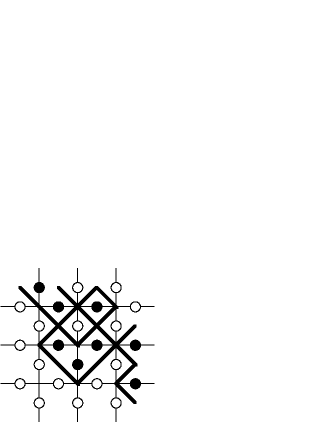
Figure 11: The Bloch walls for Ising model at high temperature. Filled dots represent states of spin $+1$ and empty dots represent states of spin $-1$. The walls separate domains of opposite spin.

Now we have a natural direction to study: the properties of Bloch walls in high temperature phases of spin models. The topological sector corresponds to the original spin variables. The non-topological one to the geometry of the Bloch walls. As another example consider the three state Potts model. There are three states per vertex, represented by empty dot, full dot or square in figure 12. The Bloch walls carry one arrow if, when one faces along the arrow, there is either (i) an empty dot on the right and a full dot on the left, or (ii) there is a square on the right and an empty dot on the left. The Bloch walls carry two arrows if there is a square is on the right and a full dot on the left of the arrows. With these rules there is obviously current conservation.

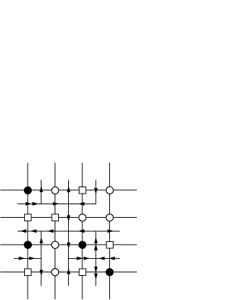
Figure 12: The Bloch walls for the three-state Potts model at high temperature. By convention the full dot, empty dot and square correspond to $\sigma=1,2,3$ respectively. The walls carry one or two arrows depending on the difference of spins between both sides. By convention the highest spin is to the right of the arrow(s).

By analogy with the foregoing Ising model, there are two natural geometrical correlation functions that are constant at large distance: the probabilities that two edges are extremities of the same open line carrying either one or two arrows. Similarly there are two natural correlation functions that decay algebraically: the probabilities that two edges belong to the same loop carrying one or two arrows. In this example there is charge conjugation symmetry that in fact relates simple and double arrows so these pairs of correlation functions are in fact identical. The obvious topological model behind this is the $SU_{1}(3)/SU_{1}(3)$ model. The fractal dimension of the contours can be reasonably conjectured to be given by the formula similar to that for the Ising model,

$$h~{}=~{}{1\over 16}-{1\over 2}\left({-{1\over 4}}\right)~{}=~{}{3\over 16}\ ,$$ (80)

leading to $D_{f}={13\over 8}$.

More generally one can conjecture similar properties for the contours in the high temperature phase of the $Z_{n+1}$ models and $SU_{1}(n+1)/SU_{1}(n+1)$ theories. The conformal weight $h$ will be $h={c\over 24}-{1\over 2}({-{c\over 6}})={c\over 8}$, where $c={3n\over n+2}$ is the central charge of the $n^{\rm th}$ $N=2$ superconformal minimal model. This leads to a predicted fractal dimension of:

$$D_{f}~{}=~{}2-{c\over 4}~{}=~{}{5n+16\over 4(n+2)}\ .$$ (81)

6 Conclusions and open problems

The subject of $N=2$ lattice models has, as yet, not produced the same kind of nice structures as in the continuum $N=2$ field theories. In particular it is important to emphasize that there is no real algebraic simplification for the computation of most physical properties. This suggests that, despite the large number of models exhibited so far, some better ones still remain to be discovered. In addition, very little is understood about the “lattice supersymmetry” and the way these $N=2$ lattice models provide discretizations of field theories with fermions. A step in that direction would be to identify supercharges on the lattice and study their anti-commutator in the scaling limit. This might be accomplished in the way that has recently been used for the Virasoro algebra [56].

On the other hand the study of $N=2$ lattice models has already provided many interesting physical ideas, in particular concerning the topological models. We believe that $N=2$ theories are the natural framework to describe most geometrical statistical mechanics models and more generally the properties of Bloch walls in non-critical spin models. It is also amusing to notice that what is “physical” in field theory and condensed matter is rather different. For instance spontaneous breaking of $N=2$ supersymmetry seems to be a very natural feature in lattice models. It is rather remarkable that the associated level crossings are encoded in the poles of differential equations of Painleve type.

While finding a lattice version of supersymmetry is probably the most important issue to resolve, there are many other open problems in the subject of $N=2$ lattice models. One can try to establish our observations about Bloch walls in generality, or find evidence to support these observations through numerical simulations. As mentionned in section 4, there are unresolved issues about supersymmetry and the scatering matrices in the more complex $N=2$ quantum integrable models. (Some suggestions about these scattering matrices have recently been made [81].) Simple corner transfer matrix computations have been done for $N=2$ lattice models [38, 82]. The results yield $N=2$ superconformal characters as one would expect, but the computation was done by the traditional method [41]. It would be interesting to see if the remarkable properties of $N=2$ supersymmetry could be exploited directly to reach this result in a much simpler manner.

There is also the question of more general lattice correlation functions. In the continuum limit, at criticality, one can obtain Knizhnik-Zamolodchikov equations for the correlation functions in $N=2$ superconformal coset models. At first sight, these equations are no simpler than those for non-supersymmetric coset models. However, once one puts in the special parameter values for the correlators of chiral primary fields one finds that one has saturated some bound and the solution of the differential equation is particularly simple. For example, if the equation is hypergeometric, the correlator of chiral primaries is usually one of the special rational solutions. It would be most interesting to see if similar simplifications occur in the $q$-deformed Knizhnik-Zamolodchikov equations for the lattice correlators of [83].

Much of the motivation for these open problems is simply to find some $N=2$ supersymmetry miracles in exactly solvable lattice models. We therefore leave it as a general challenge to find a another formulation of these models, perhaps using the Landau-Ginzburg structure more directly, in which the $N=2$ supersymmetry leads to dramatic simplifications.

Acknowledgements

One of us (N. W.) would like thank the organizers of the workshop on “New Developments in String Theory, Conformal Models and Topological Field Theory,” for their invitation to speak and for creating a very stimulating workshop. The authors also wish to thank the organizers for providing them with the opportunity to write this review, which is the result of many discussions. The authors wish to thank warmly their collaborators, in particular Paul Fendley, Dennis Nemeschansky, Alyosha Zamolodchikov and Ziad Maassarani. This work was partially supported by the DOE under grant No. DE-FG03-84ER40168. H. S. was also supported by the Packard Foundation.

References

- [1] E. Martinec, “Criticality, catastrophes and compactifications,” in the V.G. Knizhnik memorial volume, L. Brink et al. (editors): “Physics and mathematics of strings.”
- [2] N.P. Warner, Lectures on superconformal theories and singularity theory”,in “Superstrings ’89,” proceedings of the Trieste Spring School, 3–14 April 1989. Editors: M. Green, R. Iengo, S. Randjbar-Daemi, E. Sezgin and A. Strominger. World Scientific (1990); “ Supersymmetric Integrable Models and Topological Field Theories,” Lectures given at the Summer School on High Energy Physics and Cosmology, Trieste, Italy, June 15th – July 3rd, 1992. To appear in the proceedings.
- [3] C. Vafa, Lectures given at the Summer School on High Energy Physics and Cosmology, Trieste, Italy, June 15th – July 3rd, 1992. To appear in the proceedings.
- [4] E. Martinec, Phys. Lett. 217B (1989) 431; C. Vafa and N.P. Warner, Phys. Lett. 218B (1989) 51.
- [5] W. Lerche, C. Vafa and N.P. Warner, Nucl. Phys. B324 (1989) 427.
- [6] A. Cappelli, C. Itzykson and J.B. Zuber, Nucl. Phys. B280 (1987) 445.
- [7] E. Witten, Nucl. Phys. B403 (1993) 159; “On the Landau-Ginzburg description of minimal models,” IASSNS-HEP-93-10, hep-th/9304026.
- [8] P. di Francesco, O. Aharony and S. Yankielowicz, “Elliptic Genera and the Landau-Ginzburg approach to orbifolds,” SACLAY-SPHT-93-068, hep-th/9306157.
- [9] T. Kawai, Y. Yamada and S.-K. Yang, “Elliptic genera and superconformal field theory,” KEK-TH-362, hep-th/9306096.
- [10] M. Henningson, “ gauged WZW models and the elliptic genus,” IASSNS-HEP-93-39, hep-th/9307040.
- [11] P. Fendley, S. Mathur, C. Vafa and N.P. Warner, Phys. Lett. 243B (1990) 257.
- [12] P. Fendley and K. Intriligator, Nucl. Phys. B372 (1992) 533; Nucl. Phys. B380 (1992) 265.
- [13] A. LeClair, D. Nemeschansky and N.P. Warner Nucl. Phys. B390 (1993) 653.
- [14] S. Cecotti and C. Vafa, Nucl. Phys. 367 (1991) 359.
- [15] S. Cecotti, P. Fendley, K. Intriligator and C. Vafa, Nucl. Phys. B386 (1992) 405.
- [16] V. Pasquier, Nucl. Phys. B295 (1988) 491.
- [17] V. Pasquier and H. Saleur, Nucl. Phys. B330 (1990) 523.
- [18] B. Nienhuis, J. Stat. Phys. 34 (1984) 731.
- [19] P. di Francseco, H. Saleur and J.-B. Zuber, J. Stat. Phys. 49 (1987) 57.
- [20] P. Di Francesco, H. Saleur and J.-B. Zuber, Nucl. Phys. B285 (1987) 454; Nucl. Phys. B300 (1988) 393; I. Kostov, Nucl. Phys. B300 (1988) 559. J.-B. Zuber, “Conformal Field Theories, Coulomb Gas Picture and Integrable models”, in Fields, Strings and Critical Phenomena, editors E. Brézin and J. Zinn-Justin, Les Houches 1988 Session XLIX.
- [21] E. Date, M. Jimbo, T. Miwa and M. Okada, Phys. Rev. B35 (1987) 2105.
- [22] D. Friedan, Z. Qiu and S. Shenker, Phys. Lett. 151B (1984) 1575.
- [23] D. Kastor, E. Martinec and S. Shenker, Nucl. Phys. B316 (1989) 590.
- [24] Z. Qiu, Nucl. Phys. B270 (1986) 205.
- [25] O. Foda, Nucl. Phys. B300 (1988) 611.
- [26] S.-K. Yang, Nucl. Phys. B285 (1987) 183.
- [27] S.-K. Yang and H.B.Zheng, Nucl. Phys. B285 (1987) 410.
- [28] M. Baake and G. von Gehlen, V.Rittenberg, J. Phys. A20 (1987) L479; J. Phys. A20 (1987) L487.
- [29] P. di Francesco, H. Saleur and J.-B. Zuber, Nucl. Phys. B300 (1988) 393.
- [30] S.-K. Yang, Phys. Lett. B209 (1988) 242.
- [31] H. Saleur, Nucl. Phys. B382(1992) 486, 532.
- [32] A.G. Izergin and V.E. Korepin, Commun. Math. Phys. 79 (1981) 303.
- [33] S.O. Warnaar, M.T. Batchelor and B. Nienhuis, J. Phys. A25 (1992) 3077.
- [34] P. Fendley and H. Saleur, Nucl. Phys. B388 (1992) 609.
- [35] C. Gomez and G. Sierra, “Spin anisotropy commensurable chains: quantum group symmetries and Susy,” Nucl. Phys. B, to appear.
- [36] Z. Maassarani, D. Nemeschansky and N.P. Warner, Nucl. Phys. B393 (1993) 523.
- [37] Z. Maassarani, “Conformal Weights via Bethe Ansatz for Superconformal Theories,” USC preprint USC-93/019.
- [38] D. Nemeschansky and N.P. Warner, “Off-Critical Lattice Analogues of Supersymmetric Quantum Integrable Models,” preprint USC-93/018, to appear in Nucl. Phys. B.
- [39] P. Kasteleyn and C. Fortuin, J.Phys. Soc. Japan Suppl. 26 (1969) 11.
- [40] H.W.J. Blote and M.P.M. Nightingale, Physica 112A (1982) 405.
- [41] R.J. Baxter, “Exactly solved models in statistical mechanics,” Academic Press, London 1982.
- [42] P. Martin, “Potts models,” World Scientific.
- [43] P. Martin and H. Saleur,“The blob algebra and the periodic Temperley-Lieb algebra”, preprint USC-93-009, to appear in Lett. Math. Phys..
- [44] G. Felder, Nucl. Phys. B317 (1989), 215.
- [45] L.P. Kadanoff and A.C. Brown, Ann. Phys. 121 (1979) 318.
- [46] V. Pasquier, Commun. Math. Phys. 118 (1988) 335.
- [47] H. Saleur and J.-B. Zuber, “Integrable Lattice Models and Quantum Groups,” in the proceedings of the 1990 Trieste Spring School on String Theory and Quantum Gravity.
- [48] G.E. Andrews, R.J. Baxter and P.J. Forrester, J. Stat. Phys. 35 (1984) 193.
- [49] A. Kuniba and T. Yajima, J. Stat. Phys. 52 (1987) 829; P. Ginsparg, Nucl. Phys. B295 (1988) 153; P.A. Pierce and K. Seaton, Ann. Phys. 193 (1989) 326; P.A. Pierce and M.T. Batchelor, J. Stat. Phys. 60 (1990) 77.
- [50] P. Mathieu and M.A. Walton, Phys. Lett. 254B (1991) 106.
- [51] W. Lerche and N.P. Warner, Nucl. Phys. B358 (1991) 571.
- [52] M.T. Grisaru, S. Penati and D. Zanon, Phys. Lett. 253B (1991) 357; G.W. Delius, M.T. Grisaru, S. Penati and D. Zanon, Phys. Lett. 256B (1991) 164; Nucl. Phys. B359 (1991) 125.
- [53] J. Evans and T.J. Hollowood Nucl. Phys. B352 (1991) 723; Nucl. Phys. B382 (1992) 662; Phys. Lett. 293B (1992) 100.
- [54] G. Felder and A. LeClair, Int. J. Mod. Phys. A7 (1992) 239.
- [55] F. M. Goodman, P. de la Harpe, V. F. R. Jones, “Coxeter graphs and towers of algebras”, MSRI Publications number 14, Springer Verlag, and references therein.
- [56] W.M. Koo and H. Saleur, “Representations of the Virasoro algebra from lattice models,” preprint USC-93-025.
- [57] M. Takahashi and M. Suzuki, Prog.Th.Phys. 48 (1972) 2187.
- [58] Al.B. Zamolodchikov, Nucl. Phys. B366 (1991) 122; Nucl. Phys. B358 (1991) 524.
- [59] N. Yu Reshetikhin and H. Saleur,“Lattice regularization of massive and massless integrable field theories”, preprint USC-93/-20.
- [60] L.D. Faddeev and L.A. Takhtajan, Phys.Lett. A85 (1981) 375.
- [61] P. Fendley and H. Saleur, “Massless integrable QFT and massless scattering in dimensions,” preprint USC-93-022.
- [62] P.G. de Gennes, “Scaling concepts in polymer physics”, Cornell University Press.
- [63] P. Fendley, H. Saleur and Al.B. Zamolodchikov, “Massless flows I: the sine-Gordon and models” and “Massless flows II: the exact S-matrix approach”, Int. J. Mod. Phys. A, to appear.
- [64] M. Jimbo, T. Miwa and M. Okado, Commun. Math. Phys. 116 (1988) 507.
- [65] B. Duplantier and H. Saleur, Nucl. Phys. B290 (1987) 291.
- [66] Y. Kazama and H. Suzuki, Nucl. Phys. B234 (1989) 73.
- [67] D. Nemeschansky and N.P. Warner, Nucl. Phys. B380 (1992) 241.
- [68] P. Fendley, W. Lerche, S.D. Mathur and N.P. Warner, Nucl. Phys. B348 (1991) 66.
- [69] E. Witten, Commun. Math. Phys. 117 (1988) 353; Commun. Math. Phys. 118 (1988) 411; Nucl. Phys. B340 (1990) 281.
- [70] T. Eguchi and S.-K. Yang, Mod. Phys. Lett. A4 (1990) 1693.
- [71] T. Miwa, M. Jimbo and M. Okado, “Symmetric tensors of the family,” Kyoto preprint (1987), in Algebraic Analysis, Festschrift for M. Sato’s 60th birthday, Academic Press (1988).
- [72] M.P. Richey and C.A. Tracy, J. Stat. Phys. 42 (1986) 311.
- [73] E. Date, M. Jimbo, A. Kuniba, T. Miwa and M. Okado, Advanced Studies in Pure Mathematics, 16 (1988) 17.
- [74] T.R. Klassen and E. Melzer, Nucl. Phys. B338 (1990) 485.
- [75] D. Bernard and A. LeClair, Phys. Lett. 247 (1990) 309; C. Ahn, D. Bernard, and A. LeClair, Nucl. Phys. B346 (1990) 409; D. Bernard and A. LeClair, Commun. Math. Phys. 142 (1991) 99.
- [76] T. Hollowood, “A Quantum Group Approach to Constructing Factorizable S-Matrices,” Oxford Preprint OUTP-90-15P, June 1990.
- [77] T. Nakatsu, Nucl. Phys. B356 (1991) 499; H.J. de Vega and V.A. Fateev, Int. J. Mod. Phys. A6 (1991) 3221.
- [78] P. Christe and G. Mussardo, Nucl. Phys. B330 (1990) 465; Int. J. Mod. Phys. A5 (1990) 4581; G. Mussardo, Int. J. Mod. Phys. B6 (1992) 2061.
- [79] M. Karowski and H. J. Thun, Nucl. Phys. B190 (1981) 61; E. Ogievetsky and P. Wiegmann, Phys. Lett. 168 (1986), 360; E. Ogievetsky, N.Yu. Reshetikhin and P. Wiegmann, Nucl. Phys. B280 (1987) 45.
- [80] V.V. Bazhanov, N.Yu. Reshetikhin, Progress in Theor. Phys. 102 (1990) 301.
- [81] C. Gomez and G. Sierra, “On the integrability of Landau-Ginzburg models: a graph generalization of the Yang-Baxter equation,” CERN preprint TH-6963/93, hep-th/9309007.
- [82] D. Nemeschansky and N.P. Warner, in preparation.
- [83] M. Jimbo, K. Miki, T. Miwa and A. Nakayashiki, “Correlation functions of the -model for ,” kyoto PRINT-92-0191, hep-th/9205055; M. Jimbo, T. Miwa and A. Nakayashiki, J. Phys. A26 (1993) 2199; O. Foda, M. Jimbo, T. Miwa, K. Miki and A. Nakayashiki, “Vertex operators in solvable lattice models,” RIMS-922, hep-th/9305100; M. Jimbo, T. Kojima, T. Miwa, Y.-H. Quano, “Smirnov’s integrals and quantum Knizhnik-Zamolodchikov equation of level ,” RIMS-945, hep-th/9309118.