The differential geometry of Fedosov’s quantization

Abstract

B. Fedosov has given a simple and very natural construction of a deformation quantization for any symplectic manifold, using a flat connection on the bundle of formal Weyl algebras associated to the tangent bundle of a symplectic manifold. The connection is obtained by affinizing, nonlinearizing, and iteratively flattening a given torsion free symplectic connection. In this paper, a classical analog of Fedosov’s operations on connections is analyzed and shown to produce the usual exponential mapping of a linear connection on an ordinary manifold. A symplectic version is also analyzed. Finally, some remarks are made on the implications for deformation quantization of Fedosov’s index theorem on general symplectic manifolds.

1 Introduction

In a remarkable paper [9], B. Fedosov presented a simple and very natural construction of a deformation quantization for any symplectic manifold. The construction begins with a linear symplectic connection on the tangent bundle of a manifold and proceeds by iteration to produce a flat connection on the associated bundle of formal Weyl algebras. The aim of this paper is to give some geometric insight into Fedosov’s construction by exploring some of its purely classical analogs. Our basic idea is that Fedosov’s quantization procedure involves a sort of “quantum exponential mapping.”

The paper is divided into two parts. The first part (Sections 2 through 4) is mostly discursive and follows fairly closely the lecture given by the second author at the conference in honor of Bert Kostant’s 60’th birthday. The second part (Sections 5 through 8), more technical and logically self-contained, develops the proofs of some of the statements in the first part.

2 Deformation quantization and symplectic connections

The basic deformation quantization problem is to put a noncommutative (associative) product structure on the formal power series ring ${\cal A}[[\hbar]]$ over a commutative Poisson algebra ${\cal A}$. The physical origins of this particular formulation of the classical limit are obscure to this author (see Section 16.23 in [3] for an occurrence in a textbook), but the origins of its recent intensive study seem to lie in the work of Berezin [2] and Bayen et al [1].

The deformed product, which is determined by the product of elements of ${\cal A}$ and can be written in the form

$$f*_{\hbar}g=\sum_{j}\hbar^{j}B_{j}(f,g)$$

for bilinear operators $B_{j}$ on ${\cal A}$, is assumed to start with the original commutative product followed by the Poisson bracket, i.e.,

$$f*_{\hbar}g=fg+(i\hbar/2)\{f,g\}+\cdots$$

It was already noted in [1] that, when ${\cal A}$ is the algebra of $C^{\infty}$ functions on a symplectic manifold $P$, the term of order $\hbar^{2}$ in the deformed product is closely related to a torsion-free symplectic connection on $P$. If there exists such a connection which is flat, one can immediately write down a solution of the deformation quantization problem. In fact, $P$ is then covered by coordinate charts for which the transition maps are affine symplectic transformations, which leave invariant the Moyal product [1] on $C^{\infty}({\mathbb{R}}^{2n})[[\hbar]]$. (The algebra with this product is often called the (smooth) Weyl Algebra.)

When $P$ does not admit a flat symplectic connection (or where such a connection cannot be invariant under an important symmetry group, such as in the case of the hyperbolic plane with its $PSL(2,{\mathbb{R}})$ symmetry), it is necessary to “piece together” quantizations like the one above in a more elaborate way. The first such construction to work for all symplectic manifolds was that of DeWilde and Lecomte [5] who actually piece together quantizations on individual coordinate systems with nonlinear transition maps.

A more geometric formulation of the “piecing construction” was given by Maeda, Omori, and Yoshioka in [12]. Their construction has important elements in common with that of Fedosov, so we will describe it in some detail here.

For any symplectic manifold $P$, we consider its tangent bundle $TP$ with the Poisson structure for which each fibre is a symplectic leaf, carrying the translation invariant symplectic 2-form associated with its structure as a symplectic vector space. It is very simple to quantize this Poisson manifold — we simply quantize each fibre by the Moyal product, so that the noncommutative algebra $C^{\infty}(TM)[[\hbar]]$ may be identified with the set of “smooth” sections of a bundle whose fibre over each point $p$ of $P$ is the smooth Weyl algebra of the tangent space. Geometrically, we think of $C^{\infty}(TM)[[\hbar]]$ as the “space of functions on the quantized tangent bundle”.

To quantize $P$ itself, we may try to embed $C^{\infty}(P)[[\hbar]]$ as a subalgebra of this noncommutative $C^{\infty}(TP)[[\hbar]]$. The embedding onto the functions which are constant on fibres of $TP$ does not work, since this subalgebra is commutative, so we need a different embedding. In geometric terms, we are trying to replace the usual projection of $TP$ to $P$ by a different one.

To see what this new projection should look like, we may examine the simplest case, where $P$ is a symplectic vector space. Denoting by $x$ some linear coordinates on $P$ and $(x,y)$ the corresponding coordinates on $TP$, the multiplication on the quantized $TP$ is just the “Moyal product in $y,$ with $x$ as a parameter.” If we identify each function $f(x)$ on $P$ with the function $Lf(x,y)=f(x+y)$ on $TP$, then taking the fibrewise Moyal product of $Lf$ and $Lg$ reproduces the “Moyal product in $x$” of $f$ and $g$. The operator $L$ is just pullback by the map $(x,y)\mapsto(x+y),$ which is nothing but the exponential mapping of $P$ with its flat affine structure. (Here, the deformation parameter $\hbar$ just comes along for the ride.) It is not hard to see that the same idea works for any symplectic manifold with a flat, torsion–free symplectic connection: pulling back functions from $P$ to $TP$ by the exponential map allows one to pull back the multiplication on the quantized tangent bundle to get the aforementioned Moyal-type deformation quantization of $P$.

At this point, one might object that the connection on $P$ might not be complete, in which case its exponential map is not globally defined. In this case, it suffices to restrict the fibrewise Moyal product to the open subset of $TP$ which is the domain of the exponential map.

When the connection on $P$ has nonvanishing torsion or curvature, the situation is much worse, in that the set of functions pulled back from $P$ by the exponential map is not closed under the multiplication on the quantized $TP$. Two remedies for this problem have been used in the literature. We may describe them roughly as follows. In [12], the local exponential mappings coming from a covering of $P$ by Darboux coordinate systems are “patched together” to produce a new projection which is no longer (at least not manifestly) the exponential map of a connection. This new projection is built at the “quantum level”: that is, what is actually constructed is a patching together of modifications of the local pullback mappings from functions on the base to subalgebras of local sections of the bundle of Weyl algebras. In fact, this description is slightly oversimplified. It is not the bundle of smooth Weyl algebras but rather the bundle of formal Weyl algebras (formal power series around zero of functions on the tangent spaces) which must be used. Also, the parameter $\hbar$ now plays an essential role, in that the pullback of a function on the base is no longer independent of $\hbar$.

Fedosov [9], on the other hand, beginning with a linear symplectic connection having zero torsion but nonvanishing curvature, lifts it to a connection on the bundle of formal Weyl algebras and then modifies the connection on this bundle, with structure Lie algebra the inner derivations, to make it flat. He then shows how the space of parallel sections of this bundle, which is clearly a subalgebra of the algebra of all sections, may be identified with the space $C^{\infty}(P)[[\hbar]]$.

The idea which we propose in this paper is that Fedosov’s construction can also be interpreted on the level of spaces. The parallel sections of the bundle of formal Weyl algebras are defined by the vanishing of covariant differentiation operators, which are derivations on the space of sections. When the space of sections is considered as the space of functions on the quantized $TP$ (more precisely, on a formal neighborhood of the zero section in the quantized $TP$), these derivations may be thought of as vector fields, determining a distribution on $TP$ which is transverse to the fibres, i.e. an Ehresmann connection, on $TP.$ The flatness of Fedosov’s connection is equivalent to the involutivity of the distribution, or the flatness of the Ehresmann connection. Thus, the parallel sections of the formal Weyl algebra bundle are interpreted as functions on the quantized $TP$ which are constant along the leaves of the quantum foliation which is tangent to the quantum Ehresmann connection.

To pull back a function on $P,$ we first identify it with a function on the zero section, then extend it to a function on $TP$ constant along leaves. This is possible if the Ehresmann connection is not tangent to the zero section of $TP,$ but is rather transverse to the zero section, so that each leaf intersects the zero section in a unique point. To achieve this, even if the initial linear connection is flat, we must modify it by the addition of a “translation” term to obtain a connection with affine structure group.

The somewhat mysterious fact that a parallel section for the Fedosov connection is not determined by its value at a single point can also be attributed to the addition of the translational term, which changes the way in which the covariant differential operator behaves with respect to the grading in the formal Weyl algebra. In other terms, the fact is related to the non-determination of a $C^{\infty}$ function by its Taylor series at one point. An analogous situation occurs on the bundle of infinite jets of real-valued functions on $P$, which carries a “flat connection” for which the parallel sections are the infinite jets of functions on $P$. In a sense, what Fedosov’s construction does is to identify this bundle of infinite jets of functions on $P$ with the bundle of formal functions on the fibres of $TP$ and then to pull back the natural flat connection from the former bundle to the latter.

There is another way to see the necessity of “affinizing” the structure group of the connection. If a nonlinear flat connection on $TM$ has the zero section as a parallel section, then its linearization at the origin would be a flat linear connection. There are, in general, obstructions to the existence of such a connection; by allowing the zero vectors to move, we bypass these obstructions.

3 Classical analogs

In the previous section, we used geometric language to give an intuitive picture of the constructions on quantized formal power series in [9]. Now we will turn the tables and apply Fedosov’s formal constructions in purely classical settings. A more detailed version of the following remarks is contained in the second part of this paper, beginning with Section 5.

Suppose that we are simply given a differentiable manifold $P$ with a torsion free linear connection on $TP$. This connection may be lifted to a connection on the associated bundle of algebras of formal power series on the tangent spaces of $P.$ If we extend the structure group of this connection from the Lie algebra of linear vector fields on ${\mathbb{R}}^{m}$ ($m$ being the dimension of $P$) to the Lie algebra of formal vector fields, then Fedosov’s iteration method can be used to produce, in a canonical way, a flat connection on this bundle for which the corresponding Ehresmann connection is transverse to the zero section. The leaves of the foliation given by the flat Ehresmann connection are the fibres of a “mapping” from a formal neighborhood of the zero section in $TP$ to $P$. We denote this formal mapping by $\mbox{EXP}.$

On the other hand, there is another well known mapping from $TP$ to $P$ determined by a connection, namely the usual exponential mapping $\exp.$ What is the relation between these two mappings? Since both are produced in a canonical manner from the connection, it is natural to guess that they are equal. In fact this is true, as we prove below. The structure of the proof is of some interest. We first prove that, for a real-analytic connection, the flat connection given by Fedosov’s iteration is given by convergent power series, so it actually defines a flat real-analytic Ehresmann connection on a neighborhood of the zero section. In this case, we prove by following geodesics that EXP and $\exp$ coincide. Next, we show that EXP can be defined in the purely formal context by “extension by continuity,” using the fact that the convergent power series (already the polynomials) are dense in all the power series with respect to the uniformity for which two power series are close if all their coefficients up to some high degree are equal. Finally, we conclude that EXP and $\exp$ are equal since they agree on a dense subset. Since all the constructions are local, they then apply on any manifold, without any reference to a real-analytic structure.

In a sense, we have shown that the iterative procedure used by Fedosov to “flatten” a connection, when applied to ordinary manifold, is simply another way of constructing the usual exponential mapping. It is in this sense that we are tempted to say that his quantization procedure involves the pullback of functions from a symplectic manifold $P$ to its quantized $TP$ by quantization of the exponential mapping of a given symplectic connection. Before taking this leap, though, we must be more careful, because the exponential mapping of a symplectic linear connection on a symplectic manifold does NOT in general define symplectic mappings from the tangent spaces with their constant symplectic structures to the manifold with its given symplectic structure.

To produce from a symplectic torsion-free linear connection on $TP$ a symplectic nonlinear connection (on a formal neighborhood of the zero section), we must change the structure Lie algebra from the algebra of formal vector fields to the algebra of formal symplectic vector fields. In fact, with a view toward quantization, it is useful to use instead the one-dimensional extension of the latter algebra given by the infinite jets of functions, with the Poisson bracket Lie algebra structure. As is well known, this Lie algebra acts on itself by derivations of both the multiplication and the Poisson bracket. Now the iterative procedure can be applied again in this symplectic classical context to produce (formal) symplectic “exponential” mappings from the fibres of $TP$ to $P$. It would be interesting to have a more geometric construction of these mappings. Perhaps they are the same as those obtained by starting with the ordinary exponential mappings and then correcting these by using the deformation-method proof of Darboux’s theorem in [13].

4 Rigidity of quantization and Fedosov’s index theorem

In the sections above, we have concentrated on Fedosov’s construction of a deformation quantization. This construction was, however, merely the beginning of Fedosov’s work, one of whose points of culmination is an index theorem for arbitrary symplectic manifolds [8]. This theorem is a generalization of the Atiyah-Singer theorem, to which it reduces when the symplectic manifold is a cotangent bundle.

In this section, we wish to comment on the role which Fedosov’s index theorem might play in resolving a fundamental question in the general theory of deformation quantization. The condition

$$f*_{\hbar}g=fg+(i\hbar/2)\{f,g\}+\cdots$$

which describes the $\hbar$ dependence of the product $*_{\hbar}$ says nothing about how the product behaves after the deformation parameter “leaves the first-order neighborhood of zero.” This weak condition seems to contrast with the rigidity implied by the special role of rational values of $q=e^{i\hbar}$ in the theory of quantum groups. The question thus arises as to whether the dependence on $\hbar$ should be “rigidified” by some supplementary condition(s).

A possible source of such rigidity is suggested in [14], where in the special case of quantizations of Moyal type on tori with translation-invariant Poisson structures it is shown that the Schwartz kernel of the bilinear multiplication operator $*_{\hbar}$ satisfies a Schrödinger equation in which Planck’s constant plays the role of time, and the hamiltonian operator is the Poisson structure extended by translation invariance to become a differential operator on $P\times P.$ Although this kind of evolution equation for quantization may possibly extend to other situations where the notion of translation makes sense (e.g. on Lie groups), it is not at all clear how to extend it to general symplectic manifolds.

Another kind of rigidity in the deformation parameter appears in the geometric quantization of Kähler manifolds by sections of holomorphic sections of line bundles (and the extension of this quantization to general symplectic manifolds by the method of Toeplitz operators in [4]). The deformation parameter $\hbar$ then occurs as a unit by which the cohomology class of the symplectic structure (which in physical examples carries the units of action) is divided to obtain a cohomology class with numerical values which, when integral, is the first Chern class of a complex line bundle. When this class is integral for $\hbar=\hbar_{0},$ then as $\hbar$ runs over the set of values $\hbar_{0}/k$, for $k$ a sufficiently large integer, the dimension of the space of holomorphic sections is given according to the Riemann-Roch theorem by a polynomial in $k$ of degree equal to half the dimension of the symplectic manifold, which is completely determined by the cohomology class of the symplectic structure and the total Chern class of the tangent bundle for an almost complex structure compatible with the symplectic structure. This behavior shows that geometric quantization has a very rigid behavior with respect to $\hbar.$

The index theory of Fedosov [8] provides an analog in deformation quantization of the rigidity described in the preceding paragraph. According to this theory, when his deformation quantization is extended from scalar functions to matrix-valued functions on $P,$ a notion of “abstract elliptic operator” can be defined. When a suitable trace is introduced, the index of such an operator can be defined. Fedosov’s index theorem then expresses this index as a polynomial in $(1/\hbar)$ which is completely determined by the Chern character of a certain vector bundle over $P$ associated to the operator, the $\hat{A}$ class of the tangent bundle of $P$ (with an almost complex structure), and the cohomology class of the symplectic structure. Once again, this formula suggests that some quantizations (for which this formula is true) are “better” than others which might have the same first-order behavior with respect to $\hbar.$

5 Construction of formal flat connections

In this section we study in detail the classical analog of the flat connection $D$ constructed in [9] for the quantum case. In this classical setting the Weyl algebra bundle is replaced by ${\cal A}={\cal F}(TP)$, the algebra of smooth functions on $TP$, or, if one restricts oneself to the study of formal power series on the fibres, by ${\cal A}=\Gamma(\bigcup_{p\in P}{\cal J}^{\infty}_{0}(T_{p}P,{\mathbb{R}}))$, where ${\cal J}^{\infty}_{0}(T_{p}P,{\mathbb{R}})$ denotes the set of $\infty$-jets at 0 of real valued functions on $T_{p}P$. The product on ${\cal A}$ in the non-symplectic setting is either pointwise multiplication for ${\cal A}={\cal F}(TP)$, or, for ${\cal A}=\Gamma(\bigcup_{p\in P}{\cal J}^{\infty}_{0}(T_{p}P,{\mathbb{R}}))$, the mapping induced by it on the set of $\infty$-jets, respectively. In the symplectic case studied in Section 8 this product is supplemented by the fibrewise Poisson bracket (i.e., the Poisson bracket on the fibres of TP induced by the symplectic form $\omega$ on $P$), to produce a Poisson algebra structure.

Let $\Lambda(P)$ be the set of forms on $P$. The contraction $(i_{X}\alpha)(\cdot)$ is defined as $\alpha(X,\cdot)$ for a vector $X$ and a form $\alpha$. As in [9], we can define operators $\delta$ and $\delta^{-1}$ on ${\cal A}\otimes\Lambda(P)$, given in local coordinates $(x^{i})$ on $P$ and induced coordinates $(x^{i},y^{i})$ on $TP$ by:

$$\delta=dx^{i}\wedge\frac{\partial}{\partial y^{i}}$$ (1)

and

$$\delta^{-1}a=\frac{1}{p+q}\;i_{y^{i}\frac{\partial}{\partial x^{i}}}a$$ (2)

if $a$ is a $q$-form that is homogenous of degree $p$ in $y$, $p+q\neq 0$, and $\delta^{-1}a=0$ if $p=q=0$.

Let ${\cal V}^{inv}(TP)$ denote the set of invariant vertical vector fields, i.e., of vertical lifts of vector fields on $P$, We can define the operators $\delta$ and $\delta^{-1}$ on forms with values in the ‘formal vertical vector fields’ ${\cal A}\otimes{\cal V}^{inv}(TP)\otimes\Lambda(P)$ as well, by letting them act trivially on ${\cal V}^{inv}(TP)$. With this definition, the “Hodge decomposition”

$$a=a_{00}+(\delta^{-1}\delta+\delta\delta^{-1})a$$ (3)

still holds for $a\in{\cal A}\otimes{\cal V}^{inv}(TP)\otimes\Lambda(P)$. Here, $a_{00}$ denotes the homogeneous part of $a$ which is a zero-form of degree 0 in the vertical coordinates $(y^{i})$; i.e. it is simply an element of ${\cal V}^{inv}(TP)$.

We would like to construct from a given linear, torsion-free, nonflat connection $\partial$ a flat, nonlinear connection on $TP$ with structure group $\mbox{Diff}({\mathbb{R}}^{n})$ (or the symplectomorphism group of ${\mathbb{R}}^{n}$ for even $n$ in the case of the Poisson algebra studied in Section 8), or equivalently, a flat Ehresmann connection on $TP$. Locally, such a connection is represented by a one-form $X_{\mbox{\scriptsize tot}}$ on $P$ with values in the vertical vector fields, yielding for the local expression for the curvature $\Omega$, i.e., the obstruction to the integrability of the horizontal distribution defining the connection:

$$\Omega=dX_{\mbox{\scriptsize tot}}+1/2[X_{\mbox{\scriptsize tot}}\stackrel{{\scriptstyle\raisebox{-2.0pt}[0.0pt][0.0pt]{$\wedge$}}}{{,}}X_{\mbox{\scriptsize tot}}]$$

where $[\cdot\stackrel{{\scriptstyle\raisebox{-2.0pt}[0.0pt][0.0pt]{$\wedge$}}}{{,}}\cdot]$ acts as the Lie bracket on the vector part and as the exterior product on the form part of $X$. A connection induces a covariant derivative $D$ on elements of ${\cal A}$, which is given in local coordinates by:

$$Df=\left(\frac{\partial}{\partial x^{i}}f\right)dx^{i}+X_{\mbox{\scriptsize tot}}\cdot f.$$

By analogy with the quantum case in [9], $X_{\mbox{\scriptsize tot}}$ should be locally of the form

$$X_{\mbox{\scriptsize tot}}=-\frac{\partial}{\partial y^{i}}dx^{i}-\Gamma^{i}_{kl}(x)y^{k}\frac{\partial}{\partial y^{i}}dx^{l}+X,$$ (4)

where $\Gamma^{i}_{kl}(x)$ are the Christoffel symbols of the connection $\partial,$ and $X$ is at least of second degree in $y$.

The addition of the term $\frac{\partial}{\partial y^{i}}dx^{i}$, which corresponds to the operator $\delta$, corresponds to the transition from the linear connection $\partial$ to an affine connection with connection form $X_{\mbox{\scriptsize tot}}-X$ by the addition of the solder form [10]. The vanishing of the torsion for $\partial$ implies that the “translational” part of the curvature of the affine connection is zero.

For instance, if the connection $\partial$ is flat, we may choose $X\equiv 0$ in $(\ref{eq:Xansatz})$ to get a flat connection again. In this case, the original horizontal distribution corresponding to $\partial$ is already integrable. For $P={\mathbb{R}}^{n}$ with the canonical flat connection, the leaves of the horizontal distribution correponding to $\partial$ are affine subspaces ${\mathbb{R}}^{n}\times\{v\}\subset{\mathbb{R}}^{2n}$ parallel to the zero section $Z={\mathbb{R}}^{n}\times\{0\}\cong P$. This foliation is rotated by the addition of the solder form in such a way that the leaf through $(x,v)$ intersects the zero section in $(x+v,0)$ for arbitrary $(x,v)\in{\mathbb{R}}^{2n}$ (Figure 1).

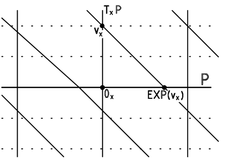
Figure 1: Addition of the solder form to a fl at linear connection “rotates” the parallel sections (from dotted to solid lines) so that they become transversal to the zero section.

In the general, non-flat case one may interpret the ansatz $(\ref{eq:Xansatz})$ as first going over from the structure group $\mbox{Gl}(n,{\mathbb{R}})$ with $n=\dim(P)$ to the affine group $\mbox{Gl}(n,{\mathbb{R}})\lhd{\mathbb{R}}^{n}$ in order to get a horizontal distribution transversal to the zero section, and then deforming it in order to get a flat nonlinear connection, which has an integrable horizontal distribution and hence defines a foliation.

Although the transition from a linear connection to an affine connection is canonical, one could in principle take any multiple of $\delta$ in order to define a generalized affine connection in the sense of [10], i.e., a connection on the $\mbox{Gl}(n,{\mathbb{R}})\lhd{\mathbb{R}}^{n}$-bundle of affine frames. However, the choice made in the ansatz is not only geometrically natural, but also distinguished by the validity of Theorem 3 and Lemma 4 below.

The requirement of the vanishing of the curvature yields the condition:

$$0=\Omega=R-\delta X+\partial X+1/2[X\stackrel{{\scriptstyle\raisebox{-2.0pt}[0.0pt][0.0pt]{$\wedge$}}}{{,}}X],$$ (5)

where $\partial X\stackrel{{\scriptstyle\mbox{\tiny{def}}}}{{=}}dX-[\Gamma^{i}_{kl}(x)y^{k}\frac{\partial}{\partial y^{i}}dx^{l}\stackrel{{\scriptstyle\raisebox{-2.0pt}[0.0pt][0.0pt]{$\wedge$}}}{{,}}X]$, and $R$ denotes the curvature tensor corresponding to $\partial$. The term $[\frac{\partial}{\partial y^{j}}dx^{j}\stackrel{{\scriptstyle\raisebox{-2.0pt}[0.0pt][0.0pt]{$\wedge$}}}{{,}}\Gamma^{i}_{kl}(x)y^{k}\frac{\partial}{\partial y^{i}}dx^{l}]$ which one would expect to appear in (5) is equal to $\Gamma^{i}_{kl}(x)dx^{j}\wedge dx^{l}\frac{\partial}{\partial y^{i}},$ which vanishes because the connection is torsion–free.

We first try to find a formal power series in $y$ for the solution of Equation (5). Solutions of this equation are not unique; however, we will show that they are in one-to-one correspondence to formal vertical vector fields $a\in{\cal A}\otimes{\cal V}^{inv}(TP)$ of degree at least 3 in $y$ via the ‘normalization condition’

$$\delta^{-1}X=a.$$ (6)

We will see in Section 6 that $\delta^{-1}X$ is just the $X$-dependent term that appears in the equation defining autoparallel curves. Hence, the case $a=0$ will prove to be special in so far as the term involving $X$ does not change autoparallel curves: in general $\delta^{-1}X$ can be interpreted as an acceleration term for autoparallel curves.

Therefore it might appear natural to admit only the special case $a=0$. However, we will see in section 8 that the boundary condition $\delta^{-1}X$ is not appropriate in the symplectic case. (It must be replaced by the condition $\delta^{-1}r=0$ for the corresponding hamiltonian function $r$.) Hence, we will admit arbitrary values of $a$ in the non-symplectic case as well.

Using $(\ref{eq:delta})$ and the vanishing of $X_{00}$ (since $X$ is a one-form), we get:

$$X=\delta a+\delta^{-1}(R+\partial X+1/2[X\stackrel{{\scriptstyle\raisebox{-2.0pt}[0.0pt][0.0pt]{$\wedge$}}}{{,}}X]),$$ (7)

which must be satisfied by any solution to $(\ref{eq:curvzero})$ and $(\ref{eq:bound})$. As in [9], this equation may be solved by iteration, yielding a unique power series for $X$. In spite of the more general normalization condition $(\ref{eq:bound})$, the argument in [9] (also see the “topological lemma” in [6]) showing that the $X$ found in this way is indeed a solution to $(\ref{eq:curvzero})$ is still valid: defining $A$ as the right hand side of equation $(\ref{eq:curvzero})$ with the recursively constructed $X$, we may check that $A$ fulfills the equation $\delta A=\partial A+[X,A]$ and the condition $\delta^{-1}A=0$ and hence vanishes identically.

Hence, we have proved the following theorem

Theorem 1

For each $a\in{\cal A}\otimes{\cal V}^{inv}(TP)$ at least of degree 3 in $y$ there is a unique formal flat connection, i.e., a solution to $(\ref{eq:curvzero})$, satisfying the normalization condition $(\ref{eq:bound})$.

6 Analytic connections and the “exponential map”

In the last section we constructed a formal flat connection from a given linear, torsion-free connection. In this section we will show that this formal power series is convergent in a tubular neighborhood $U$ of the zero section if the manifold $M$, the connection $\partial$, and the element $a$ in the normalization condition are real analytic. The proof uses the method of majorants, as discussed in any standard reference on real analytic functions, such as [11].

Theorem 2

Let $P$ be a real analytic manifold, $\partial$ an analytic linear connection, and $a\in{\cal F}(TP)$ an analytic function such that $a$ and its derivatives up to order two in the direction of the fibres vanish on the zero section $Z$. Then the formal power series which is the solution of $(\ref{eq:iter})$ obtained by iteration is convergent in a neighborhood $U$ of $Z$ and hence defines an analytic Ehresmann connection on $U\subset TP$.

Proof: Choose coordinates $(x^{i})$ on $P$ and induced coordinates $(x^{i},y^{i})$ on $TP$. We define a linear operator $T$ on power series (divisible by $y)$ in $(x,y)$ by its action on monomials in $y$:

$$Ty^{k}\phi(x)\stackrel{{\scriptstyle\mbox{\tiny{def}}}}{{=}}\frac{1}{k}y^{k}\frac{d}{dx}\phi(x)$$

We will show:

1. The power series of the components $X^{i}_{j}$ of $X=X^{i}_{j}\frac{\partial}{\partial y^{i}}dx^{j}$ are majorized by
   $f(\sum x^{i},\sum y^{i})$, where $f(x,y)$ is a power series with no terms of order zero in $y$ which is a solution of:

   $$f(x,y)=A(\frac{y^{2}}{(1-\beta x)(1-\beta y)}+yTf(x,y)+\frac{y}{1-\beta x}f(x,y)+f(x,y)^{2}).$$ (8)

   for sufficiently large $A>0$ and $\beta>0$.

2. $f(x,y)$ is convergent in a neighborhood of $(0,0)$.

Hence, $X$ is analytic.

To show 1, we first observe that Equation $(\ref{eq:major})$ has a unique solution containing no term of order zero in $y$, which can be computed by iteration.

We say that $f$ majorizes $X^{i}_{j}$ up to order $k$ in $y$ iff the absolute value of the coefficient of any monomial $x^{\mu}y^{\nu}$ in $X^{i}_{j}$ for arbitrary multiindices $\mu,\nu$ with $|\nu|\leq k$ is not larger than the respective coefficient in $f(\sum x^{i},\sum y^{i})$.

Both $X^{i}_{j}$ and $f(\sum x^{i},\sum y^{i})$ contain no terms of order zero or one in $y$. As the coefficients of any analytic function $\rho(z)=\sum_{\mu\in{\mathbb{N}}^{N}}C^{\mu}z^{\mu}$ in variables $(z^{1},\ldots,z^{N})$ have to satisfy $|C^{\mu}|<AB^{|\mu|}$ for some constants $A,B$, the function $\rho$ is majorized by $\alpha/(1-\beta(z^{1}+...+z^{N}))$ for some $\alpha,\beta>0$. From this general statement it follows that there are $\alpha,\beta$ such that the components of $\delta a+\delta^{-1}R$ are majorized by $\alpha y^{2}(1-\beta x)^{-1}(1-\beta y)^{-1}$ , and the Christoffel symbols $\Gamma^{i}_{kl}$ are majorized by $\alpha(1-\beta x)^{-1}$, where $x=\sum x^{i},y=\sum y^{i}$. Hence, from equations $(\ref{eq:iter})$ and $(\ref{eq:major})$ it is obvious that for $A>\alpha$ the power series $f(\sum x^{i},\sum y^{i})$ majorizes all $X^{i}_{j}$ up to order 2 in $y$.

Now assume that $f(\sum x^{i},\sum y^{i})$ majorizes all $X^{i}_{j}$ up to some order $k\in{\mathbb{N}}$. Then, by construction of $T$, the components of $\delta^{-1}dX$ are majorized up to order $(k+1)$ by $2NyTf(x,y)$, where $N=\dim P$. The components of $1/2[X\stackrel{{\scriptstyle\raisebox{-2.0pt}[0.0pt][0.0pt]{$\wedge$}}}{{,}}X]$ are majorized by $2N^{2}f(x,y)\frac{d}{dy}f(x,y)$ up to order $k$. Thanks to the factor $1/(p+q)$ in the definition $(\ref{eq:deltainv})$ of $\delta^{-1}$, the components of $\delta^{-1}1/2[X\stackrel{{\scriptstyle\raisebox{-2.0pt}[0.0pt][0.0pt]{$\wedge$}}}{{,}}X]$ are majorized up to order $(k+1)$ by

$$4N^{3}\int_{0}^{y}f(x,\hat{y})\frac{d}{d\hat{y}}f(x,\hat{y})d\hat{y}=2N^{3}f(x,y)^{2},$$

Finally, the components of $[\Gamma^{i}_{kl}y^{k}\frac{\partial}{\partial y^{i}}dx^{k}\stackrel{{\scriptstyle\raisebox{-2.0pt}[0.0pt][0.0pt]{$\wedge$}}}{{,}}X]$ are majorized up to order $k$ by $N^{2}\alpha/(1-\beta x)(f+y\frac{d}{dy}f)$ and $\delta^{-1}[\Gamma^{i}_{kl}y^{k}\frac{\partial}{\partial y^{i}}dx^{k}\stackrel{{\scriptstyle\raisebox{-2.0pt}[0.0pt][0.0pt]{$\wedge$}}}{{,}}X]$ is majorized up to order $(k+1)$ by

$$2N^{3}\int_{0}^{y}\alpha/(1-\beta x)(f(x,\hat{y})+\hat{y}\frac{d}{d\hat{y}}f(x,\hat{y}))d\hat{y}=2N^{3}\alpha/(1-\beta x)yf$$

Hence, by equations $(\ref{eq:iter})$, $(\ref{eq:major})$, $X^{i}_{j}$ is majorized up to order $(k+1)$ in $y$ by $f(\sum x^{i},\sum y^{i})$, and 1 is shown.

To prove 2 we show, again by induction on the degree in $y$, that $f$ is majorized by the solution $g(x,y)$ which has no terms of degree zero or one in $y$ of the purely algebraic equation

$$g(x,y)=\tilde{A}(\frac{y^{2}}{(1-\beta x)(1-\beta y)}+2\frac{y}{1-\beta x}g(x,y)+g(x,y)^{2}),$$ (9)

where $\tilde{A}=\beta A$ if $\beta>1$, and $\tilde{A}=A$ otherwise. Obviously, $g$ majorizes $f$ up to order $2$. Furthermore, by iteration of equation $(\ref{eq:major2})$, $g$ has the property that the coefficient of $y^{k}$ consists of a sum of terms of the form $a/(1-\beta x)^{l}$ with $a\in{\mathbb{R}}^{+},l\in{\mathbb{N}},l\leq k$. Assume that $f$ is majorized by $g$ up to order $k$ in $y$. As

$$yT\frac{y^{k}}{(1-\beta x)^{l}}=\frac{l}{k}\frac{\beta y}{1-\beta x}\frac{y^{k}}{(1-\beta x)^{l}}$$

$yTf(x,y)$ is majorized up to order $(k+1)$ by $\beta yg(x,y)/(1-\beta x)$, and hence, by equations $(\ref{eq:major})$, $(\ref{eq:major2})$, $f$ is majorized by $g$ up to order $(k+1)$, so $f$ is majorized by $g$.

The solutions to the quadratic equation $(\ref{eq:major2})$ are

$$g(x,y)=-\frac{1}{2}\left(2\frac{y}{1-\beta x}-\frac{1}{\tilde{A}}\right)\pm\sqrt{\frac{1}{4}\left(2\frac{y}{1-\beta x}-\frac{1}{\tilde{A}}\right)^{2}-\frac{y^{2}}{(1-\beta x)(1-\beta y)}}.$$

Both solutions are obviously analytic functions in $(x,y)$, as the argument of the square root is an analytic function with nonvanishing zeroth degree term, the solution with the minus sign being the desired solution, which starts with a term quadratic in $y$. Hence $f$ is majorized by a convergent power series, and 2 is shown. Q.E.D.     

Since the Ehresmann connection defined by $X$ is flat, the horizontal distribution is integrable. Due to the $\delta$-term in $(\ref{eq:Xansatz})$, this distribution is transversal to the zero section $Z$, and for a sufficiently small tubular neighborhood $U\subset TP$ of $Z$ each leaf in $U$ intersects $Z$ in exactly one point. Hence, we can define an “exponential mapping” $\mbox{EXP}_{p}:T_{p}P\cap U\rightarrow P$ for any $p\in P$ which maps $v_{p}$ to the unique intersection point of the leaf through $v_{p}$ and the zero section in $TP$ (Figure 2).

Figure 2: The “exponential mapping” for a flat linear connection is found by following parallel sections from the fibres to the zero section.

With this definition, the normalization condition $(\ref{eq:bound})$ with $a=0$ is distinguished by the following theorem:

Theorem 3

The mappings $\mbox{EXP}_{p}$ and the usual exponential mappings $\exp_{p}$ coincide on $U\cap T_{p}P$ for all $p\in P$ iff the choice $\delta^{-1}(X)=0$ is made in (6).

Proof: To prove the theorem, we first observe that $X$ determines a natural notion of autoparallel curves: Any curve $\gamma$ in $P$ may be lifted to a curve in $TP$ by taking the derivative $\dot{\gamma}$. A curve $\gamma$ is called autoparallel iff $\dot{\gamma}$ is horizontal, i.e., tangent to the horizontal distribution defining the connection.

In local coordinates, this condition is of the form:

$$\ddot{x}^{i}(t)=-\dot{x}^{i}(t)-\Gamma^{i}_{kl}(x)\dot{x}^{k}\dot{x}^{l}a+X^{i}_{k}(x,\dot{x})\dot{x}^{k}~{}~{},$$ (10)

where $X^{i}_{k}(x,y)\frac{\partial}{\partial y^{i}}dx^{k}$ is the local coordinate expression for $X$.

The connection between autoparallel curves and the ‘exponential mapping’ EXP is particular simple in the case of $P={\mathbb{R}}^{n}$ with the standard flat connection $\partial$ (Figure 1). In this case, the equation for autoparallel curves is just $\ddot{x}^{i}(t)=-\dot{x}^{i}(t)$ with the solution

$$\dot{x}(t)=\dot{x}(0)e^{-t},~{}~{}~{}x(t)=x(0)+\dot{x}(0)(1-e^{-t}).$$

The term $-\dot{x}^{i}(t)$ coming from the $\delta$-term in $X_{\mbox{\scriptsize tot}}$ can be interpreted as a friction term slowing the particle down as it approaches the zero section (Figure 1). In particular, $EXP(x(0),v(0))=\lim_{t\rightarrow\infty}x(t)=x(0)+v(0)$, and $EXP$ coincides with the usual exponential mapping of the connection $\partial$. In the general case, the interpretation of the first term on the right hand side of $(\ref{eq:dgl})$ as a friction term is still valid.

Note that the last term in $(\ref{eq:dgl})$ is precisely $\delta^{-1}(X)$. Suppose that this is zero. Then a reparametrization $t\leadsto-\log(1-\tau)$ yields the usual geodesic equation corresponding to the connection $\partial$ for $\tilde{x}(\tau)\stackrel{{\scriptstyle\mbox{\tiny{def}}}}{{=}}x(-\log(1-\tau))$. In particular, for sufficiently small initial velocity $v$, $\tilde{x}(\tau)$ is defined for $0\leq\tau\leq 1$, and $x(t)$ is defined for $0\leq t<\infty$.

As $\lim_{t\rightarrow\infty}\tau(t)=\lim_{t\rightarrow\infty}(1-e^{-t})=1$, we get: $\lim_{t\rightarrow\infty}x(t)=\lim_{\tau\rightarrow 1}\tilde{x}(\tau)=\exp(v)$ with $v=\dot{x}(0)$. On the other hand, by construction the curve $(x,\dot{x})(t)$ in $TP$ is contained in the leaf of the horizontal foliation through $v$. As $\lim_{t\rightarrow\infty}\dot{x}(t)=\lim_{t\rightarrow\infty}e^{-t}\frac{d}{d\tau}\tilde{x}(\tau)=0$, $\lim_{t\rightarrow\infty}x(t)$ is just the intersection point of the leaf through $v$ and the zero section, i.e. $\mbox{EXP}(v)$. Hence, $\mbox{EXP}(v)=\exp(v)$ and we have proved that the condition $\delta^{-1}(X)=0$ is sufficient for the maps EXP and $\exp$ to coincide.

To prove the converse we assume $\mbox{EXP}_{p}=\exp_{p}$ for all $p\in P$, and $\delta^{-1}X$ arbitrary. We first show the following lemma:

Lemma 4

Let $\gamma$ be a geodesic corresponding to the connection $\partial$, $\tilde{\gamma}:{\mathbb{R}}\rightarrow P$ the reparametrized geodesic: $t\mapsto\gamma(1-e^{-t})$, i.e., a solution to the differential equation

$$\ddot{x}^{i}(t)=-\dot{x}^{i}(t)-\Gamma^{i}_{kl}(x)\dot{x}^{k}\dot{x}^{l}.$$ (11)

Then, for all $t$:

$$\exp_{\tilde{\gamma}(t)}\left(\dot{\tilde{\gamma}}(t)\right)=\exp_{\tilde{\gamma}(0)}\left(\dot{\tilde{\gamma}}(0)\right)=\lim_{t\rightarrow\infty}{\tilde{\gamma}(t)}$$

Remark: The lemma says that a solution of $(\ref{eq:dgl_noX})$ is a reparametrized geodesic that is slowed down by the ‘friction term’ $-\dot{x}$ just to that extent that $\exp(\dot{\tilde{\gamma}}(t))$ is constant.

Proof of the lemma:

Denote by $\gamma_{2}$ the geodesic starting at $\tilde{\gamma}(t_{0})$ with initial velocity $\dot{\tilde{\gamma}}(t_{0})$ for some fixed time $t_{0}$. As follows from the first part of the proof of theorem 3 above, $\tilde{\gamma}_{2}(t)=\gamma_{2}(1-e^{-t})$ defines again a solution of $(\ref{eq:dgl_noX})$. Obviously, this solution is obtained from $\tilde{\gamma}$ by a constant shift in time, as $\dot{\tilde{\gamma}}_{2}(0)=\dot{\tilde{\gamma}}(t_{0})$. Hence, $\lim_{t\rightarrow\infty}\tilde{\gamma}(t)=\lim_{t\rightarrow\infty}\tilde{\gamma}_{2}(t)$. On the other hand, we have already proved that $\lim_{t\rightarrow\infty}\tilde{\gamma}(t)=\exp_{\tilde{\gamma}(0)}(\dot{\tilde{\gamma}}(0))$ (and hence $\lim_{t\rightarrow\infty}\tilde{\gamma}_{2}(t)=\exp_{\tilde{\gamma}_{2}(0)}(\dot{\tilde{\gamma}}_{2}(0))$), so the lemma follows. Q.E.D.     

Using this lemma we will finish the proof of Theorem 3, i.e., we will show that the condition $\delta^{-1}X=0$ is a necessary condition for the maps EXP and $\exp$ to coincide.

Assume that the curve $t\mapsto\frac{d}{dt}\gamma(1-e^{-t})$ in $TP$ is not completely contained in the leaf through $v_{q}$, where $\gamma:t\mapsto\gamma(t)$ is a geodesic of $\partial$ with $\gamma(0)=v_{q}$ for an arbitrary $v_{q}\in TP$. By continuity there is a open subset $O\subset{\mathbb{R}}$ such that $w(t):=\frac{d}{dt}\gamma(1-e^{-t})$ is not contained in the leaf through $v_{q}$ for any $t\in O$. By assumption and the lemma, $\mbox{EXP}(w(t))=\exp(w(t))=\exp(v_{q})=\mbox{EXP}(v_{q})$, so we get an infinity of different leaves intersecting the zero section in the same point, in contradiction to the transversality of the horizontal distribution.

Hence, the curve $t\mapsto\frac{d}{dt}\gamma(1-e^{-t})$ is completely contained in the leaf through $v_{q}$, i.e., it is a horizontal curve, and therefore must fulfill both equations $(\ref{eq:dgl})$ and $(\ref{eq:dgl_noX})$. Obviously, this is only possible if the difference between the two equations vanishes, i.e.,

$$X^{i}_{k}(x,\dot{x})\dot{x}^{k}\equiv 0\Leftrightarrow\delta^{-1}X=0,$$

and Theorem 3 is proved. Q.E.D.    

Remark: Even when $\delta^{-1}X\neq 0$, the equality $\mbox{EXP}(v)=\lim_{t\rightarrow\infty}x(t)$, where $x(t)$ is the solution of $(\ref{eq:dgl})$ with $\dot{x}(0)=v$, still holds. To prove this statement we show that the ‘friction term’ in $(\ref{eq:dgl})$ insures that $\lim_{t\rightarrow\infty}\dot{x}(t)=0$ for sufficiently small initial velocity $v$. However, this is easy to see: Multiplying $(\ref{eq:dgl})$ by $\dot{x}^{i}$ and summing over $i$, we get:

$$\frac{1}{2}\frac{d}{dt}\sum_{i}\dot{x}^{i}\dot{x}^{i}=-\sum_{i}\dot{x}^{i}\dot{x}^{i}-\sum_{i}\dot{x}^{i}\left(\Gamma^{i}_{kl}(x)\dot{x}^{k}\dot{x}^{l}+X^{i}_{k}(x,\dot{x})\dot{x}^{k}\right)$$

As $X$ has degree at least two in $y$, for sufficiently small velocity

$$|\sum_{i}\dot{x}^{i}\left(\Gamma^{i}_{kl}(x)\dot{x}^{k}\dot{x}^{l}+X^{i}_{k}(x,\dot{x})\dot{x}^{k}\right)|<\epsilon\sum_{i}\dot{x}^{i}\dot{x}^{i}$$

for some $\epsilon$ with $0<\epsilon<1$.

Hence,

$$(-1-\epsilon)\sum_{i}\dot{x}^{i}\dot{x}^{i}<\frac{1}{2}\frac{d}{dt}\sum_{i}\dot{x}^{i}\dot{x}^{i}(-1+\epsilon)\sum_{i}\dot{x}^{i}\dot{x}^{i},$$

$$e^{-2(1+\epsilon)t}\sum_{i}\dot{x}^{i}(0)\dot{x}^{i}(0)<OA\sum_{i}\dot{x}^{i}(t)\dot{x}^{i}(t)<e^{-2(1-\epsilon)t}\sum_{i}\dot{x}^{i}(0)\dot{x}^{i}(0),$$

and

$$\lim_{t\rightarrow\infty}\dot{x}(t)=0$$

but the curve $(x(t),\dot{x}(t))$ does not intersect the zero section at a finite time.

7 The formal exponential map

In the last section we have shown how to construct the mapping EXP in the analytic case, where the formal flat connection was convergent and defined a flat Ehresmann connection in the usual sense on some neighborhood of the zero section. In the non-analytic case we cannot expect the series for $X$ to be convergent. However, we will show that we can define a formal exponential map, i.e., an $\infty$-jet of mappings from the fibre $T_{p}P$ to $P$, and we will show that for this map Theorem 3 still holds, if we replace $\exp_{p}$ by its $\infty$-jet as well.

In order to define the formal exponential map we first show the following lemma for real-analytic manifolds:

Lemma 5

Let $P$ be a real-analytic manifold, $\partial$ an analytic connection and $a$ an analytic function, $X$ the solution of $(\ref{eq:curvzero})$ with the normalization condition $(\ref{eq:bound})$. Then the $k$-jet of $\mbox{EXP}_{p}$ at $0_{p}\in T_{p}P$ for arbitrary $k\in{\mathbb{N}},p\in P$ is completely determined by the $k$-jet at $p$ of the connection form corresponding to $\partial$ and the $(k+1)$-jet at $0_{p}$ of $a$.

Proof: It is sufficient to consider some small neighborhoods $V\subset P$ of $p\in P$ and $TV\subset TP$ of $0_{p}\in T_{p}P$. We choose coordinates $(x^{i})$ on $V$ and show first that the $k$-jet of $\mbox{EXP}_{p}$ is determined by the $k$-jet of $X$.

By the definition of the map $\mbox{EXP}_{p}$, we may compute the components $\mbox{EXP}_{p}^{i}$ of $\mbox{EXP}_{p}$ in the chosen coordinate system by taking the covariant constant continuation $f^{i}$ to $TV\subset TP$ of the coordinate functions $x^{i}$ and restricting them to the fibre $T_{p}P$:

$$\mbox{EXP}_{p}^{i}(y)=f^{i}(y)\;\rule[-5.69054pt]{0.56905pt}{14.22636pt}_{\;T_{p}P}$$

with

$$Df^{i}=0,~{}~{}~{}~{}~{}f^{i}\;\rule[-5.69054pt]{0.56905pt}{14.22636pt}_{\;Z}=x^{i},$$

where $Z$ denotes the zero section in $TP$.

As the constructed connection is flat, we know that such functions $f^{i}$ exist. Rather than constructing them by the iterative procedure of [9], we will use a more geometric approach. The condition $Df^{i}=0$ reads locally:

$$\frac{\partial}{\partial x^{k}}f^{i}+M^{m}_{k}\frac{\partial}{\partial y^{m}}f^{i}=0,$$ (12)

where $M$ is the matrix with elements

$$M^{m}_{k}=\delta^{m}_{k}+\Gamma^{m}_{jk}y^{j}-X^{m}_{k},$$ (13)

where $\delta^{m}_{k}$ equals $1$ if $m=k$, and $0$ otherwise. Due to the $\delta^{m}_{k}$ coming from the solder form the matrix valued function $M$ is invertible, and the inverse $M^{-1}$ is analytic at $0_{p}$ again. Furthermore, its $k$-jet at $0_{p}$ only depends on the $k$-jet of $M$ at $0_{p}$.

Hence, we can solve (12) for $\frac{\partial}{\partial y^{k}}f^{i}$ yielding

$$\frac{\partial}{\partial y^{k}}f^{i}+(M^{-1})^{m}_{k}\frac{\partial}{\partial x^{m}}f^{i}=0,$$ (14)

where the zero-jet of $M^{-1}$ at $0_{p}$ is just the unit matrix. $f^{i}$ is given for $y=0$, and we know that this set of partial differential equations has a unique solution, since the connection is flat. To compute it, we can integrate the differential equations successively: The equation for $\frac{\partial}{\partial y^{1}}f^{i}$ determines $f^{i}$ on the $y^{1}$-axis, the equations for $\frac{\partial}{\partial y^{k}}f^{i}$ with $1\leq k\leq m$ determine $f^{i}$ on the subspace spanned by the first $m$ basis vectors. In each step the solution is an analytic function on the respective subspace, depending analytically on the initial conditions, by the Cauchy-Kovalevskaya theorem. Hence, $f^{i}$ is analytic at $0_{p}$. Furthermore, by comparing coefficients, we see that the $k$-jet of $f^{i}$ only depends on the $k$-jet of $M^{-1}$, and hence of $M$.

Since the operator $\delta^{-1}$ contains a factor $y^{i}$, it follows from the iteration formula $(\ref{eq:iter})$ for $X$ that the $k$-jet of $X$ is determined by the $k$-jets of the Christoffel-symbols $\Gamma^{i}_{jk}$ of $\partial$ and the $(k+1)$-jet of $a$. By the definition $(\ref{eq:defM})$ this is true for $M$ as well, and the lemma is proved. Q.E.D.     

Using this lemma, we can define a formal exponential map in the non-analytic case: We use the topology on the $\infty$-jets generated by the basis of open sets consisting of sets of $\infty$-jets whose $k$-jets agree for some $k\in{\mathbb{N}}$, i.e., a sequence $(j^{i})$ of $\infty$-jets converges to an $\infty$-jet $j$, if for any $k\in{\mathbb{N}}$ there is an $N(k)\in{\mathbb{N}}$ auch that the $k$-jets of $j^{r}$ and $j$ agree for $r>N(k)$.

In this topology the set of $\infty$-jets of analytical functions forms a dense subset of the set of all $\infty$-jets. (The polynomials are already dense.) Hence, we can define the $\infty$-jet $j^{\infty}_{p}(\mbox{EXP}_{p})$ of EXP at $p$ in the non-analytic case by the continous continuation to all $\infty$-jets of the map that assigns to the pair $(\partial,j^{\infty}_{p}(a))$, consisting of an analytic connection and the $\infty$-jet of an analytic function $a$ defining the normalization condition for $X$, the $\infty$-jet $j^{\infty}_{p}(\mbox{EXP}_{p})$. This continuation exists and is unique by Lemma 5.

Theorem 6

Theorem 3 still holds in the non-analytic case, if we replace $\mbox{EXP}_{p}$, and $\exp_{p}$ by their $\infty$-jets.

Proof: If we impose the normalization condition $(\ref{eq:bound})$ with $a=0$ the direct statement of the theorem is an immediate consequence of Theorem 3, Lemma 5, and the fact that the $\infty$-jets of analytic functions are dense in the chosen topology.

To show the converse, we use the fact that $j^{\infty}_{p}(\exp_{p})$ coincides with $j^{\infty}_{p}(\mbox{EXP}_{p})$ for the choice $a=0$ in $(\ref{eq:bound})$ by the first part of the theorem. We denote for the moment the corresponding $X$ by $X^{0}$. Now, assume that the $k$-jet of $a$ in $(\ref{eq:bound})$ is different from zero for some $k>2$. Then, by $(\ref{eq:iter})$, the $(k-1)$-jet of $X$ and $X^{0}$ are different as well. This implies, that the $(k-1)$-jets of $M$ and $M^{-1}$ in $(\ref{eq:Dexp}),(\ref{eq:Dexpinv})$ are different from those for $a=0$, so the $(k-1)$-jets of the corresponding jets $j^{\infty}_{p}(\mbox{EXP}_{p})$ are different. Q.E.D.     

8 Flat symplectic connections

So far, we have studied the problem of constructing a flat connection for an arbitrary manifold $P$, without any additional structure. However, if we are interested in getting closer to the quantum case, then $P$ should be a classical phase space with its symplectic structure, and ${\cal F}(P)$ a Poisson algebra.

In this case, the Weyl-algebra bundle of [9] is replaced by ${\cal A}={\cal F}(TP)$ (or ${\cal A}=\Gamma(\bigcup_{p\in P}{\cal J}^{\infty}_{0}(T_{p}P,{\mathbb{R}}))$) with the fibrewise Poisson-structure $\{,\}_{\mbox{\scriptsize fib}}$. The flat connection must be compatible with this additional structure, i.e., the following equation should hold for all $f,g\in{\cal A}$:

$$D\{f,g\}_{\mbox{\scriptsize fib}}=\{Df,g\}_{\mbox{\scriptsize fib}}+\{f,Dg\}_{\mbox{\scriptsize fib}}.$$ (15)

Hence, $\partial$ has to be a symplectic connection and $X(v)$ has to be a symplectic vector field on $T_{x}P$ for any $v\in T_{x}P$. As the fibres are vector spaces, $X$ must be globally hamiltonian, i.e., there must be an ${\cal A}$-valued one-form $r$ such that the components of the one form $r$ are minus the hamiltonian functions of the components of the vector-valued one-form $X$. (The minus sign is chosen in order to guarantee that the Lie bracket of $X$ with itself corresponds to the Poisson bracket of $r$ with itself.)

In this case, the normalization condition $\delta^{-1}X=0$ is in general not admissible, as it will not give a symplectic vector field. This statement is an immediate consequence of the fact that the usual exponential mapping of a symplectic connection is generally not a local symplectomorphism, and the following theorem:

Theorem 7

The mapping $\mbox{EXP}(p)$ is a local symplectomorphism iff $X(v)$ is a hamiltonian vector field for any $v\in TP.$

Proof: Let $X(v)$ be a hamiltonian vector field for any $v\in TP$, with $X=X_{r}$ for some ${\cal A}$-valued one-form $r$. Then $D$ is of the form:

$$Da=\partial a+\{\omega_{ij}y^{i}dx^{j},a\}_{\mbox{\scriptsize fib}}+\{r,a\}_{\mbox{\scriptsize fib}},$$

and has the property $(\ref{eq:Dderiv})$.

We have to show:

$$\mbox{EXP}_{p}^{*}\{f,g\}=\{\mbox{EXP}_{p}^{*}f,\mbox{EXP}_{p}^{*}g\}_{p}$$ (16)

for all $f,g\in{\cal F}(P)$, where $\{,\}_{p}$ is the Poisson bracket on the fibre $T_{p}P$ induced by the constant symplectic form $\omega(p)$, i.e., the restriction of $\{,\}_{\mbox{\scriptsize fib}}$ to the fibre $T_{p}P$.

For any $a\in{\cal F}(P)$ let $\sigma(a)$ denote the unique covariant constant continuation of $a$, i.e., $\sigma(a)\in{\cal A}$, $D\sigma(a)=0,\sigma(a)\;\rule[-5.69054pt]{0.56905pt}{14.22636pt}_{\;P\subset TP}=a$, where we have identified $P$ with the zero section in $TP$.

By construction of EXP we have:

$$\mbox{EXP}_{p}^{*}f=\sigma(f)\;\rule[-5.69054pt]{0.56905pt}{14.22636pt}_{\;T_{p}P}.$$ (17)

Obviously, due to the $\delta$-term in $X_{\mbox{\scriptsize tot}}$, $\sigma(a)$ is locally of the form:

$$\sigma(a)(x,y)=a(x)+\frac{\partial}{\partial x^{i}}a(x)y^{i}+O(y^{2})$$

and hence:

$$\{\sigma(f),\sigma(g)\}_{\mbox{\scriptsize fib}}\;\rule[-5.69054pt]{0.56905pt}{14.22636pt}_{\;P}=\{f,g\},~{}~{}~{}~{}~{}D\{\sigma(f),\sigma(g)\}_{\mbox{\scriptsize fib}}=0~{}~{}~{}~{}~{}~{}~{}(\mbox{by (\ref{eq:Dderiv}))}$$

$$\Rightarrow\{\sigma(f),\sigma(g)\}_{\mbox{\scriptsize fib}}=\sigma(\{f,g\})$$

for any $f,g\in{\cal F}(P)$ by uniqueness of the covariant constant continuation of a function in ${\cal F}(P)$. Using $(\ref{eq:exp})$, equation $(\ref{eq:sympl})$ follows. Q.E.D.      

For a given linear symplectic connection the set of its nonlinear “flattenings” satisfying $(\ref{eq:Dderiv})$ is in one-to-one correspondence with the functions $f\in{\cal A}$ at least of degree 4 in the fibres by the condition: $\delta^{-1}r=f$, where $r$ is the unique one form in ${\cal A}\otimes\Lambda(P)$ which is a hamiltonian for $X$ and vanishes on $P\subset TP$. Indeed, as any $X$ is at least of second degree in the vertical coordinates, $r$ is at least of third, and $\delta^{-1}r$ at least of fourth degree.

On the other hand, given $f$, we may write the analog of equation $(\ref{eq:iter})$ for $r$ instead of $X$, which is essentially the same (up to signs, since X is minus the hamiltonian vector field of $r$, and the replacement of the commutator of vector fields by the Poisson bracket of functions.) Hence, given $f$, we can uniquely construct $r$ as the solution of the equation:

$$0=\hat{R}-\delta r+\partial r+1/2\{r,r\}.$$ (18)

with the condition

$$\delta^{-1}r=f,$$ (19)

where the ${\cal A}$-valued two-form $\hat{R}$ is the hamiltonian for the curvature $R$ considered as a two form on $P$ with values in the vertical vector fields on $TP$, locally given by $\hat{R}=(1/4)\omega_{ij}R^{j}_{klm}y^{i}y^{k}dx^{k}dx^{m}$. This solution may again be iteratively computed:

$$r=\delta f+\delta^{-1}(\hat{R}+\partial r+1/2\{r,r\}).$$ (20)

We observe that the connection on $U\subset TP$ can be easily reconstructed from the mapping EXP: The leaf through any $0_{p}\in TP$ is given by $\bigcup_{q\in P}\mbox{EXP}_{q}^{-1}(\{0_{p}\})$, and the connection is defined by the tangent distribution to those leaves. Since the mappings $\mbox{EXP}_{p}$ for different symplectic connections $\partial$ and different ‘normalization conditions’ $(\ref{eq:rcond})$ are all local symplectomorphisms, this observation implies the following theorem:

Theorem 8

The different Ehresmann connections constructed from different symplectic connections and different choices of $f$ are related by fibrewise symplectomorphism, i.e., by a section in the bundle $\bigcup_{p\in P}\mbox{\it Sym}^{\,0_{p}}(T_{p}P)$ where $\mbox{\it Sym}^{\,0_{p}}(T_{p}P)$ denotes the group of (infinite jets of) symplectomorphisms of $T_{p}P$ with fixed point $0_{p}\in T_{p}P$.

This statement is the symplectic analog of Theorem 4.3 in [9] for the quantum case, which states that two different ‘abelian connections’ $D,\tilde{D}$ are related by some inner automorphism $U$ such that $\tilde{D}=D-[DU\circ U^{-1},\cdot]$. (The theorem is formulated only for the normalization condition $\delta^{-1}r=0$. However, this condition is not used in the proof, so it is valid for the more general normalization conditions studied by us as well.)

For the condition $\delta^{-1}r=0$, EXP is in a suitable sense a ‘minimal deformation’ of the usual exponential mapping such that the resulting mapping is symplectic: namely, as the symplectic connection $\partial$ defines a splitting of $TTP$ in horizontal and vertical subspaces, we can define the accelaration $a(v_{p})$ of autoparallel curves due to $X$ and the friction term $-\delta$ at a point $v_{p}\in TP$ as the difference of the tangent vectors to the lifted autoparallel curve and the lifted geodesic corresponding to $\partial$ through that point, which is always a vertical vector. We identify $T(T_{p}P)$ and $T_{p}P$, and denote by $\uparrow$ the vertical lift: $\uparrow:T_{p}P\rightarrow T(T_{p}P),~{}~{}v\mapsto v^{\uparrow}$. In order to avoid notational confusion, we denote by $\tilde{\omega}_{p}$ the symplectic form on the vector space $T_{p}P$ induced by the symplectic form $\omega$ on $P$.

Theorem 9

The condition $\delta^{-1}r=0$ for a solution of $(\ref{eq:rcurv})$ is equivalent to the requirement that the acceleration $a(v_{p})$ is contained in the $\tilde{\omega}_{p}$-complement of $v_{p}^{\uparrow}$ for all $p\in P,v_{p}\in T_{p}P$, i.e, $\tilde{\omega}_{p}(v_{p}^{\uparrow},a(v_{p}))=0~{}\forall v_{p}\in TP$.

Proof: Any solution $r$ of $(\ref{eq:rcurv})$ is of the form $(\ref{eq:riter})$ for some $f$. $a(v_{p})$ may be written as

$$a(v_{p})=-v_{p}^{\uparrow}+a^{X}(v_{p}),$$

where the first term comes from the friction term $-\delta$ and $a^{X}(v_{p})$ is the acceleration due to $X$. For arbitrary $f$, we conclude from $(\ref{eq:dgl})$ that $a^{X}(v_{p})$ is just $(\delta^{-1}X)(v_{p})$, which is nonzero even if $\delta^{-1}r=0$, as $\delta^{-1}$ explicitly contains the vertical coordinates $y$.

Using the definition of $\delta^{-1}$ we get:

$$\delta^{-1}X=\frac{I+1}{I}X_{\delta^{-1}r}+(\omega^{\#}(I^{-1}r))^{\uparrow},$$ (21)

where $X_{f}$ denotes the hamiltonian vector field on the fibres of $TP$ corresponding to $f$ (i.e., $\tilde{\omega}^{\#}(d_{y}f)$), and $\frac{I+1}{I},I^{-1}$ are linear operators acting on monomials in $y$ of total degree $i$ by multiplication with $\frac{i+1}{i}$ and $i^{-1}$, respectively.

By $(\ref{eq:riter})$ $r$ is of the form $r=\delta f+\delta^{-1}\alpha$ for a two form $\alpha\in{\cal A}\otimes\Lambda(P)$.

Setting $V_{p}=\sum y^{i}\frac{\partial}{\partial x^{i}}$ and using $(\ref{eq:delXr})$ we get:

$$\tilde{\omega}_{p}(\delta^{-1}X,V_{p}^{\uparrow}) = \tilde{\omega}(\frac{I+1}{I}X_{f},V_{p}^{\uparrow})+\tilde{\omega}(\omega(p)^{\#}(I^{-1}(\delta f+\delta^{-1}\alpha))^{\uparrow},V_{p}^{\uparrow})$$

$$= (\delta f)(V_{p})+(\frac{1}{I}\delta^{-1}\alpha)(V_{p})$$

$$= (\delta f)(V_{p}),$$

where the last equality holds because for each monomial in $y$, the expression $(\delta^{-1}\alpha)(V_{p})$ is — up to a real factor — just $\alpha(V_{p},V_{p})=0$. Hence, $\tilde{\omega}_{p}(v_{p}^{\uparrow},a(v_{p}))=0~{}~{}\forall v_{p}\in TP$ is fulfilled for $f\equiv 0$.

On the other hand, since $(\delta f)(v_{p})=\frac{d}{d\lambda}f(x,\lambda y)\;\rule[-5.69054pt]{0.56905pt}{14.22636pt}_{\;\lambda=1}$, it follows from the fact that

$$\tilde{\omega}_{p}(v_{p}^{\uparrow},a(v_{p}))=0~{}~{}\forall v_{p}\in TP$$

that $f(x,y)$ has to be independent of $y$ and hence zero, as the constant term in $f$ must vanish. Q.E.D.

References

- [1] Bayen, F., Flato, M., Fronsdal, C., Lichnerowicz, A., and Sternheimer, D., Deformation theory and quantization, I and II, Ann. Phys. 111, (1977), 61-151.
- [2] Berezin, F.A., Quantization, Math USSR Izv. 8 (1974), 1109-1165.
- [3] Bohm, D., Quantum Theory, Prentice-Hall, New York, 1951.
- [4] Boutet de Monvel, L., and Guillemin, V., The spectral theory of Toeplitz operators, Annals. of Math. Studies 99, Princeton University Press, Princeton, 1981.
- [5] De Wilde, M., and Lecomte, P., Existence of star-products and of formal deformations of the Poisson Lie algebra of arbitrary symplectic manifolds, Lett. Math. Phys. 7 (1983), 487-496.
- [6] Donin, J., On the quantization of Poisson brackets, Advances in Math. (to appear).
- [7] Fedosov, B., Formal quantization, Some Topics of Modern Mathematics and their Applications to Problems of Mathematical Physics (in Russian), Moscow (1985), 129-136.
- [8] Fedosov, B., Index theorem in the algebra of quantum observables, Sov. Phys. Dokl. 34 (1989), 318-321.
- [9] Fedosov, B., A simple geometrical construction of deformation quantization, J. Diff. Geom. (to appear).
- [10] Kobayashi, S., and Nomizu, K., Foundations of differential geometry, Interscience, New York, 1963.
- [11] Krantz, S.G., and Parks, H.R., A Primer of Real Algebraic Functions, Basler Lehrbücher vol. 4, Birkhäuser, Basel, 1992.
- [12] Omori, H., Maeda, Y., and Yoshioka, A., Weyl manifolds and deformation quantization, Advances in Math. 85 (1991), 224-255.
- [13] Weinstein, A., Symplectic manifolds and their lagrangian submanifolds, Advances in Math. 6 (1971), 329-346.
- [14] Weinstein, A., Classical theta functions and quantum tori, Publ. RIMS Kyoto Univ., (to appear).