Measuring Small Distances in
$N$=2 Sigma Models

Abstract

We analyze global aspects of the moduli space of Kähler forms for $N$=(2,2) conformal $\sigma$-models. Using algebraic methods and mirror symmetry we study extensions of the mathematical notion of length (as specified by a Kähler structure) to conformal field theory and calculate the way in which lengths change as the moduli fields are varied along distinguished paths in the moduli space. We find strong evidence supporting the notion that, in the robust setting of quantum Calabi-Yau moduli space, string theory restricts the set of possible Kähler forms by enforcing “minimal length” scales, provided that topology change is properly taken into account. Some lengths, however, may shrink to zero. We also compare stringy geometry to classical general relativity in this context.

1 Introduction

Geometrical concepts play a central role in our theoretical descriptions of the fundamental properties of elementary particles and the spacetime arena within which they interact. The advent of string theory has reinforced this reliance on geometrical methods; it has done so, though, with a fascinating twist. String theory necessitates the introduction of particular modifications of standard geometrical constructions which can drastically modify their properties when the typical length scales involved approach Planckian values. Conversely, when all length scales involved are large compared to the Planck scale, these modified geometrical constructs approach their classical counterparts. This phenomenon of string deformed classical geometry is usually referred to as “quantum geometry” (although “stringy geometry” might be more accurate since our concern will be exclusively at string tree level).

Recently [1, 2, 3], a striking property of quantum geometry was uncovered in the context of string theory compactified on a Calabi-Yau  space. A classical analysis instructs us to limit our attention to Riemannian metrics on such a space – that is, to positive definite bilinear forms mapping $T_{X}\times T_{X}$ to ${\mathchoice{\mbox{\bbbfont R}}{\mbox{\bbbfont R}}{\mbox{\smallbbbfont R}}{\mbox{\tinybbbfont R}}}^{+}$. As Calabi-Yau spaces are Kähler, this condition can be rephrased as the statement that the Kähler form on the Calabi-Yau space $X$ lies in a subset of $H^{2}(X,{\mathchoice{\mbox{\bbbfont R}}{\mbox{\bbbfont R}}{\mbox{\smallbbbfont R}}{\mbox{\tinybbbfont R}}})$ known as the Kähler cone. However, an analysis based on string theory reveals a different story. Namely, it was shown in [1, 2, 3] that the physics of string theory continues to make perfect sense even if we allow the “Kähler form” to take values outside of the Kähler cone. This was shown, for example, to give rise to physical processes resulting in a change in the topology of the Calabi-Yau target space – processes which classical reasoning would forbid.

Another striking aspect of quantum geometry is the apparent existence of a minimum length set by the string scale $\alpha^{\prime}$. The evidence for this has come from a variety of studies. First, it has long been known [4] that string theory compactified on a circle of radius $R$ is physically identical to the theory compactified on a circle of radius $\alpha^{\prime}/R$. The full set of physically distinct possibilities with this topology is therefore parameterized by radii $R$ varying from $(\alpha^{\prime})^{1/2}$ to $\infty$; in this sense $(\alpha^{\prime})^{1/2}$ is a minimum length in this setting. Additional evidence for a minimum length was given in [5] in which the one dimensional space of Kähler forms on the quintic threefold was studied by means of mirror symmetry. Those authors found that physically distinct theories are again characterized by Kähler forms which attain a minimal nonzero volume. From another point of view, the work of [6] showed that there appears to be a smallest length scale that can be probed via high energy scattering with an extended object such as a string. Roughly, unlike what happens in the point particle case, increasing the energy of the string probe beyond a critical value results in an increase in the size of the probe itself and hence a decrease in the length scale of sensitivity.

At first sight, the observations in the last two paragraphs might seem to be at odds. On the one hand, we have mentioned work which establishes that string theory relaxes constraints on the Calabi-Yau metric and hence makes all of $H^{2}(X,{\mathchoice{\mbox{\bbbfont R}}{\mbox{\bbbfont R}}{\mbox{\smallbbbfont R}}{\mbox{\tinybbbfont R}}})$ available for consistent physical models. On the other hand, we have referred to work which establishes that string theory restricts the physically realizable metrics to a subset of those which are classically allowed. One of the main purposes of the present paper is to study this issue in some detail and show the harmonious coexistence of these apparently divergent statements.

As part of the analysis in the sequel is somewhat technical, it is worthwhile for us to briefly summarize our results here. To do so, let us first recall that in [1, 2, 3] it was shown that string theory instructs us to pass from the moduli space of Kähler forms on a single Calabi-Yau space to the enlarged Kähler moduli space. The latter is a space which comes equipped with a decomposition into cells, each of which corresponds to a different “phase” of the $N=2$ superconformal theory (see figure 1). From a mathematical point of view, one might say the walls between these cells correspond to Kähler forms which degenerate in some manner. Some of these phases are interpretable in terms of strings on (birationally equivalent but possibly topologically distinct) smooth Calabi-Yau manifolds, some other phases correspond to strings on singular (orbifold) Calabi-Yau spaces and yet other phases include Landau-Ginzburg theories and exotic hybrid combinations. More precisely, each cell contains a neighbourhood of a distinguished “limit” point (marked with a dot in figure 1) around which some kind of perturbation theory converges and the above identifications can unambiguously be made. (For the Calabi-Yau phases, these are known as “large radius limit” points.) The region of convergence is shown by a dotted line in figure 1. A generic path in this enlarged Kähler moduli space corresponds to a family of well defined conformal theories and hence there is no obstruction to passing from one cell into another. This gives rise to the topology changing transitions mentioned earlier. Under mirror symmetry, this enlarged Kähler moduli space corresponds to the complex structure moduli space of the mirror. As discussed in [2], the badly behaved conformal field theories form a subspace of complex codimension one (as opposed to the real codimension one walls in the Kähler space) in an appropriate compactification of the moduli space, which under mirror symmetry corresponds to the “discriminant locus” of the complex structure moduli space. As this locus has real codimension two, a generic path in that moduli space avoids it. This is, in fact, how we established that the same must be true for a generic path in the enlarged Kähler moduli space of the original Calabi-Yau manifold.

Figure 1: The cell decomposition of part of the moduli space.

Taking this picture at face value, it appears that some points in figure 1 correspond to Kähler forms with zero or even negative volumes (since we pass outside of a single classical Kähler cone). One superficial way of treating this is simply to assert that a geometrical interpretation can only be given to a subset of points in the moduli space — those points with a large positive volume according to some birational model of the space. Although that point of view avoids the obvious difficulties about negative volumes, our goal in this paper is to probe the issue more deeply and determine to what extent we can give a consistent geometrical interpretation (and hence assign a positive volume) to all points in the enlarged moduli space. A crucial ingredient in such a study is the precise definition of “volume” or “size” in the conformal field theory context. As the size of a space is an inherently classical mathematical notion, there is no unique way of extending its definition to quantum geometry. There are, however, a couple of compelling extensions which are both natural from the point of view of conformal field theory and which reduce to the standard notion of size in the appropriate large radius limits. One of these extensions relies upon mirror symmetry to rewrite the moduli space of Kähler forms on $X$ as the moduli space of complex structures of another space $Y$. The coordinates in this moduli space (which are coupling constants in the action of the associated conformal field theory) are then used to represent the size of $X$ in the simplest possible way (as we will discuss). This turns out to be equivalent to measuring “size” by using the classical Kähler form on the nonconformal linear $\sigma$-model which was studied in [3].

The second version of size is derived directly from properties of the conformal nonlinear $\sigma$-model. This definition can be obtained by requiring that it not only approach the notion of size based upon the classical Kähler form at the large radius limit, but also that it exactly match that notion in a certain neighbourhood of this limit. (This neighbourhood will be the region in which we can, at least in principle, calculate the conformal $\sigma$-model correlation functions and thus use the $\sigma$-model as the link between points in the moduli space and the geometry of $X$.) The measurement of size is then analytically continued in a natural way beyond this neighbourhood of the large radius limit point. In practice we will analyze this second definition of size by means of the first definition in the preceding paragraph, and of a function which relates the two sizes. This function can be expressed in terms of solutions to a set of differential equations — the Picard-Fuchs equations.

The “sizes” on which we focus in this paper will be described by specifying an area for every holomorphically embedded Riemann surface $C$ in $X$, or more generally, for every $2$-cycle $C$ on $X$. We will refer to such a specification of areas as a measure on $X$, and we will give precise definitions of the “algebraic measure” (the first notion of size) and the “$\sigma$-model measure” (the second notion of size) later in the paper.

The areas that we specify only depend on the homology class of the Riemann surface. If we choose $2$-cycles $C_{i}$ forming an integral basis of $H_{2}(X)$, and let $e^{i}$ be the dual basis of $H^{2}(X)$ then associating something like a complexified Kähler form $B+iJ=\sum t_{i}e_{i}$ to each conformal field theory in the moduli space, we see

$$\mathop{\rm Area}\nolimits(C_{i})=\mathop{\rm Im}\nolimits\int_{C_{i}}(B+iJ)=\mathop{\rm Im}\nolimits(t_{i}).$$ (1)

One should note that although our moduli space usually contains theories corresponding to many topologically distinct birational models of $X$, we can sensibly define $H_{2}(X)$ across the whole moduli space. When we do this for a Riemann surface $C_{i}$ which has positive area in the neighbourhood of the large radius limit of one model $X_{1}$, the same Riemann surface $C_{i}$ may have negative area near the large radius limit of some other model $X_{2}$. This happens for the ${\mathchoice{\mbox{\bbbfont P}}{\mbox{\bbbfont P}}{\mbox{\smallbbbfont P}}{\mbox{\tinybbbfont P}}}^{1}$’s which are flopped when passing between these models [7]. Thus what we consider to be positive or negative area depends on which $X_{i}$ we use as our starting point.

One of the results strongly indicated (but not fully proven) by the present work is that for any point $(t_{1},\ldots,t_{n})$ representing a conformal field theory, the associated areas are non-negative when we calculate them using the $\sigma$-model measure for a suitable choice of $X_{i}$. In other words, every conformal field theory in the enlarged Kähler moduli space has non-negative areas with respect to the large radius definition of size specified by at least one of the smooth birational models of $X$ (and the method of continuation given above). This is the resolution of the apparent conflict mentioned above that we put forth here (and is pictorially illustrated later in figure 6). Notice that this representation of the enlarged Kähler moduli space still has all of the phases which string theory instructs us to include (thereby enlarging the classical Kähler moduli space of a single smooth Calabi-Yau manifold) but that on the union of these phase regions, the areas are constrained to be larger than certain minimum values (thereby reducing the classical Kähler moduli space).

We note that the first evidence for this conclusion in the Calabi-Yau context can be extracted from [5]. Following [2, 3], the analog of figure 1 for the enlarged Kähler moduli space on the quintic threefold is a ${\mathchoice{\mbox{\bbbfont P}}{\mbox{\bbbfont P}}{\mbox{\smallbbbfont P}}{\mbox{\tinybbbfont P}}}^{1}$ divided into two cells by the equator, with north and south poles removed. This can be thought of as arising from ${\mathchoice{\mbox{\scrfont M}}{\mbox{\scrfont M}}{\mbox{\smallscrfont M}}{\mbox{\tinyscrfont M}}}=H^{2}(X,{\mathchoice{\mbox{\bbbfont C}}{\mbox{\bbbfont C}}{\mbox{\smallbbbfont C}}{\mbox{\tinybbbfont C}}})/H^{2}(X,{\mathchoice{\mbox{\bbbfont Z}}{\mbox{\bbbfont Z}}{\mbox{\smallbbbfont Z}}{\mbox{\tinybbbfont Z}}})$ in the natural exponential coordinates [1, 3] where, as dictated by string theory, we place no restriction on the one dimensional imaginary part of this expression. The description of [2, 3] then shows that the upper hemisphere (including arbitrary positive imaginary values in M) corresponds to the smooth Calabi-Yau phase while the lower hemisphere (including arbitrary negative imaginary values in M) corresponds to the Landau-Ginzburg phase. The analysis of [5], however, shows that if we use the $\sigma$-model definition of size (based on analytically continuing the Kähler form from the smooth Calabi-Yau region as indicated above), there is a positive lower limit on the size for all conformal theories in this enlarged moduli space. In the present work we extend this notion to more complicated moduli spaces which exhibit many qualitatively new features. Some of the regions of the moduli space we will explore can also be described in terms of classical ideas of general relativity. We will compare the classical version with the stringy description obtained in this paper.

In section 2 we will review the local structure of the moduli spaces of interest to this work. This analysis will tell us how to describe the Kähler moduli space in terms of the algebraic structure of the underlying conformal field theory — effectively by using mirror symmetry. In section 3 we will look at the global structure of the resulting moduli space. The discussion here will complement that of [2] in which toric methods were used to describe the enlarged Kähler moduli space (and by mirror symmetry complex structure moduli space as well). Here our discussion will also use toric methods, but will naturally originate in complex structure moduli space. In particular, we will see that the discriminant locus (which may be thought of as the subspace of “bad” conformal field theories) is closely related to a fan structure which in turn provides data for a natural compactification of the moduli space.

In section 4 we will discuss various ways of defining the “size” of a conformal field theory. Mathematically, this amounts to putting coordinates on the enlarged Kähler moduli space to determine a way of measuring areas at each point of the moduli space. It will be seen that two notions of area measurement arise. The first notion comes from the natural coordinates that were put on the moduli space in its algebraic toric construction. As we shall mention, these are also the coordinates which naturally arise in the $N$=2 supersymmetric gauge theories employed in [3]. The other method of area measurement comes directly from the Kähler form of the $\sigma$-model as sketched above.

The main quantitative portion of the present work concerns presenting methods for the calculation of this $\sigma$-model measure in section 5 for various boundary or limit points of the enlarged Kähler moduli space. By studying these extreme points in the moduli space we anticipate that our calculations will be sensitive to the extreme values of volumes that can physically arise. In section 6 we discuss the consequences of these calculations and present concluding remarks.

2 Local Structure of the Moduli Space

In much of what follows in both this and subsequent sections, we will use the tool of mirror symmetry and freely interchange one perspective with that of the mirror. To avoid confusion when we do so, let us state our notation clearly at the outset. Let $X$ and $Y$ be a mirror pair of Calabi-Yau manifolds. The mirror map takes (chiral,chiral)-fields into (antichiral,chiral)- fields and vice versa. For both $X$ and $Y$, we will associate deformations of the complex structure with deformations of the ring of (chiral,chiral)-fields, and thus associate deformations of the Kähler form with deformations of the ring of (antichiral,chiral)-fields. Since we ultimately wish to focus on deformations of the Kähler form of $X$ in the later sections we use $x^{i}$ to denote an (antichiral,chiral)-field in the $X$ model and $y^{j}$ to denote a (chiral,chiral)-field in the same model. These are reversed by the mirror map for the $Y$ model. This notation is summarized in table 1.

Deformations	Type	$X$	$Y$
Kähler form	(a,c)	$x^{i}$	$y^{j}$
Complex structure	(c,c)	$y^{j}$	$x^{i}$

Table 1: Notation for the fields generating the deformations of

the mirror pair of Calabi-Yau manifolds $X$ and $Y$.

We begin with the nonlinear $\sigma$-model given by embeddings, $u:\Sigma\to Y$, of a Riemann surface $\Sigma$ into a compact Kähler manifold $Y$ of complex dimension 3:

$$S=\frac{i}{4\pi\alpha^{\prime}}\int\left\{g_{i\bar{\jmath}}(\partial u^{i}\bar{\partial}u^{\bar{\jmath}}+\bar{\partial}u^{i}\partial u^{\bar{\jmath}})-iB_{i\bar{\jmath}}(\partial u^{i}\bar{\partial}u^{\bar{\jmath}}-\bar{\partial}u^{i}\partial u^{\bar{\jmath}})\right\}\,d^{2}z,$$ (2)

where $u^{i}$ are holomorphic coordinates on $Y$ pulled back to $\Sigma$ and $g_{i\bar{\jmath}}$ are the components of the pull-back of the Kähler form. The $B$-field is a closed real 2-form on $Y$. We will assume that $h^{2,0}(Y)=0$ so that the cohomology class of any closed 2-form $B$ can be represented as a $(1,1)$-form $B={\textstyle\frac{i}{2}}B_{i\bar{\jmath}}\,du^{i}\wedge du^{\bar{\jmath}}$. (In (2) we also use $B_{i\bar{\jmath}}$ to indicate the pull-back to $\Sigma$ of the components of $B$.) The extra degrees of freedom introduced by the $B$-field appear to be essential to fully understand the structure of the moduli space of this $\sigma$-model.

This $\sigma$-model may be made into an $N$=2 field theory by introducing for each $i$ a chiral superfield (in both the left-moving and right-moving sense) on $\Sigma$, $x^{i}$, whose lowest component is $u^{i}$. Introducing superspace coordinates $\theta^{\pm}$ for left-movers and $\bar{\theta}^{\pm}$ for right-movers one can show that [8] the following action

$$S=\frac{1}{4\pi^{2}\alpha^{\prime}}\left\{\int{K}(x^{i},x^{\bar{\jmath}})\,d^{4}\theta d^{2}z+2\pi i\int_{\Sigma}u^{*}(B)\right\}$$ (3)

yields (2) as its bosonic part if $g_{i\bar{\jmath}}=\frac{2i}{\pi}\frac{\partial^{2}{K}}{\partial x^{i}\partial x^{\bar{\jmath}}}$. ${K}$ is a real symmetric function of $x^{i}$ and $x^{\bar{\jmath}}$, defined only locally on the target space.

The field theory given by (3) is not necessarily conformally invariant. The conditions for conformal invariance can be studied [9, 10] by means of $\sigma$-model perturbation theory where one assumes that $\alpha^{\prime}/R^{2}\ll 1$, where $R$ is some characteristic radius of $Y$. This condition is called the “large radius limit” and its precise meaning should become clear later in this paper. To leading order in $\alpha^{\prime}/R^{2}$ one finds that conformal invariance can be achieved if $B$ is harmonic and $g_{i\bar{\jmath}}$ is Ricci-flat. Thus $Y$ is a Calabi-Yau manifold.

Given any large radius Calabi-Yau manifold we can therefore associate to it a conformal field theory given by (3). The chiral fields $x^{i}$ of this theory have simple multiplication properties [11] since one is free to make naïve definitions such as

$$(x^{i})^{2}(z)=\lim_{w\to z}x^{i}(w)x^{i}(z).$$ (4)

This simple structure for the algebra of the fields $x^{i}$ is the key to being able to use the algebraic methods later in this paper. In this paper we will often abuse notation and use $x^{i}$ to represent what is really its lowest component $u^{i}$. This is because the algebraic structure in the conformal field theory given by (4) directly translates into a statement about complex coordinates in algebraic geometry.

The moduli space of these theories can now be analyzed locally as was done in [12]. The key point is that the moduli space naturally splits into a product of two factors. Deformations of the metric, $g_{i\bar{\jmath}}$ can be divided into two types. Firstly there are deformations of the complex structure of $Y$. These do not preserve the (1,1)-type of $g_{i\bar{\jmath}}$ and introduce $g_{ij}$ and $g_{\bar{\imath}\bar{\jmath}}$ components. Such deformations form a moduli space of complex dimension $h^{2,1}(Y)$. The deformations of the metric that preserve its (1,1)-type can be combined with deformations of $B$ to form the other factor in the moduli space. This part of the moduli space can be regarded as the set of “complexified Kähler forms” $B+iJ\in H^{1,1}(Y)$, where $J$ is the Kähler form associated to $g_{i\bar{\jmath}}$, and it has complex dimension $h^{1,1}(Y)$. We will tend to drop the word “complexified” and refer to the combination $B+iJ$ itself as the “Kähler form” on $Y$. We will also fix our units of length so that $4\pi^{2}\alpha^{\prime}=1$. Note then that changing $B$ by adding an element of $H^{2}(Y,{\mathchoice{\mbox{\bbbfont Z}}{\mbox{\bbbfont Z}}{\mbox{\smallbbbfont Z}}{\mbox{\tinybbbfont Z}}})$ to it will have no effect on the field theory given by (3) and so $B+iJ$ is best thought of as an element of the quotient space $H^{1,1}(Y)/H^{2}(Y,{\mathchoice{\mbox{\bbbfont Z}}{\mbox{\bbbfont Z}}{\mbox{\smallbbbfont Z}}{\mbox{\tinybbbfont Z}}})$.

As an alternative to describing everything in terms of the intrinsic geometry of $Y$, in some cases one can embed $Y$ as a hypersurface in an ambient space with simpler geometric properties. This will allow us to go some way to naturally splitting the deformations of complex structure and Kähler form in terms of the action. Consider the action (3) on some space $Y_{1}$ with the addition of other terms:

$$S=\int{K}(x^{i},x^{\bar{\jmath}})\,d^{4}\theta d^{2}z+\int\lambda W(x^{i})\,d^{2}\theta^{+}d^{2}z+\int\bar{\lambda}\overline{W}(x^{\bar{\imath}})\,d^{2}\theta^{-}d^{2}z+2\pi i\int_{\Sigma}u^{*}(B),$$ (5)

where $\lambda$ is a new chiral superfield and $W(x^{i})$ is a holomorphic function. This action also has $N$=2 supersymmetry. Since no world-sheet derivatives of the field $\lambda$ appear we may integrate it out from its equations of motion. Integrating out the lowest component of $\lambda$ forces the condition

$$W(u^{i})=0.$$ (6)

Let us call the subspace of $Y_{1}$ given by (6) the space $Y$. Integrating out the fermionic components of $\lambda$ forces the fermionic components of $x^{i}$ to lie in the tangent bundle of the space $Y$ defined by (6). And integrating out the highest component of $\lambda$ introduces an extrinsic curvature term which along with the curvature of $Y_{1}$ produces the curvature of $Y$ much along the lines of [13]. Thus one sees that the field theory given by (5) on $Y_{1}$ is equivalent to (3) on $Y\subset Y_{1}$. It follows that the condition for conformal invariance of (5) to leading order is that the subspace $Y$ (rather than $Y_{1}$) should be Ricci-flat. Indeed, one approach [11] (coming from the ideas of [14]) to obtaining a conformal field theory from this construction is to put no condition on the metric on $Y_{1}$ and then consider the conformal field theory as the infra-red renormalized limit of (5).

In many cases all of the deformations of the complex structure of $Y$ can now be considered as deformations of the function $W(x^{i})$ rather than of the metric on the ambient space. Since this is an algebraic question we have simplified the problem. In general one might have some deformations of complex structure which cannot be expressed as deformations of $W(x^{i})$ [15] and we will indeed be treating examples where this does happen. In such a case we will ignore those “extra” deformations and so we will only really be treating a slice of the moduli space. There are examples known [16] where a topological class of a Calabi-Yau manifold can be treated by more than one model of the form (5). It can turn out [17] that in one model some deformations of complex structure can be thought of deformations of $W(x^{i})$ whereas in another model the same deformations cannot. Because of this fact one would expect that there is nothing special about the deformations we are ignoring and that we should be able to see all the salient properties of the moduli space by just looking at the slice of $W(x^{i})$-type deformations.

Consider the case where $Y_{1}$ is a complex projective space with, say, the Fubini-Study metric. The infra-red limit of the action (5) describes a conformal $\sigma$-model on the projective variety $Y$. Note however that the $x^{i}$’s are affine rather than homogeneous coordinates on $Y_{1}$. It was shown in [18] that a change of variables can absorb $\lambda$ into the superpotential $W(x^{i})$ and turn the affine coordinates into homogeneous coordinates. Such a change of variables also produced a discrete group of identifications such that the action (5) is an orbifold of the equivalent action written in homogeneous coordinates. Similar results are also obtained when $Y_{1}$ is a weighted projective space (or even a more general toric variety) and the resulting $x^{i}$ coordinates are quasi-homogeneous coordinates. From now on, to improve notation, we will rewrite the coordinates $x^{i}$ as $x_{i}$. Since these will always be coordinates in some flat affine space (of which the weighted projective space or toric variety is a quotient [19]), no confusion should arise.

Recently, Witten [3] has analyzed Calabi-Yau $\sigma$-models and their relationship to Landau-Ginzburg theories. This analysis has played a crucial role in understanding the phase structure of these theories as discussed in our introductory remarks. It also helps to clarify why algebraic methods suffice for understanding particular sectors of moduli space, as we now indicate.

In Witten’s approach, one begins with the action for an $N$=2 supersymmetric two dimensional quantum field theory with a nontrivial gauge group, which for ease of exposition we temporarily take to be $U(1)$. The action for this theory is

$$S=\int f_{\rm kin}(x_{i},y_{j})\,d^{4}\theta d^{2}z+t\int f_{\rm FI}(y_{j})\,d\theta^{+}d\bar{\theta}^{-}d^{2}z+\int W(x_{i})\,d^{2}\theta^{+}d^{2}z+\hbox{h.c.},$$ (7)

where $f_{\rm kin}(x_{i},y_{j})$ and $f_{\rm FI}(y_{j})$ (the Fayet-Illiopoulos $D$-term) are functions which we will not concern ourselves with in this paper.

One can then study this theory for various values of the parameter $t=r+i\theta$. As shown in [3], for $r$ large and positive, this theory is a $\sigma$-model  on the Calabi-Yau space given by $W=0$ in a suitable weighted projective space. For $r$ large (in absolute value) and negative, the theory is interpretable as an orbifold of a Landau-Ginzburg theory with superpotential $W$. In the infra-red limit, these quantum field theories are expected to become conformal sigma models and conformal Landau-Ginzburg theories, respectively. Mathematically, the physical construction just reviewed corresponds to building various target spaces via symplectic quotients [3]. The parameter $r$ can then be interpreted as setting the size, or more precisely, the Kähler form on the resulting space. In more general examples [3], the number of $t$ parameters equals the dimension of $H^{1,1}$ of the associated Calabi-Yau space. One of the results of the present study is to make geometrical sense of such “Kähler forms” which a superficial analysis suggests will become negative on part of the parameter space. We will return to a discussion of the $t$ coordinates and these issues shortly.

As is well known [20, 11, 21, 3], at the conformal limit, some of the equations of motion of (7) yield

$$\frac{\partial W}{\partial x_{i}}=0.$$ (8)

The important point for our purposes is that if we assume that all the deformations of the complex structure of $Y$ are encoded in the function $W(x_{i})$, we can study the complex structure moduli space using algebraic methods. Namely, the fields $x_{i}$ obey the multiplication rules of the chiral ring [11]

$${\mathchoice{\mbox{\scrfont R}}{\mbox{\scrfont R}}{\mbox{\smallscrfont R}}{\mbox{\tinyscrfont R}}}=\frac{{\mathchoice{\mbox{\bbbfont C}}{\mbox{\bbbfont C}}{\mbox{\smallbbbfont C}}{\mbox{\tinybbbfont C}}}[x_{0},x_{1},\ldots]}{\left(\frac{\partial W}{\partial x_{0}},\frac{\partial W}{\partial x_{1}},\ldots\right)},$$ (9)

where $(I_{1},I_{2},\ldots)$ represents the ideal generated by $I_{1},I_{2},\ldots$. In the case that $Y$ is 3-dimensional, this ring encodes much of the information concerning the 3-point functions in the conformal field theory.

Because the $x_{i}$ are (quasi-)homogeneous coordinates, or equivalently because they are charged under the $U(1)$ symmetries of the $N$=(2,2) algebra, the ring R is graded. Elements of the ring with left and right charge (1,1) may be added to $W(x_{i})$ in the action (7) to give another valid theory. Such fields thus form truly marginal operators.

We will now attempt to describe the deformations of Kähler form in the same language. We will begin by describing the deformations of the complex structure of a Calabi-Yau threefold $X$ by describing $X$ as the zero locus of a holomorphic function $V(y_{j})$ in some ambient space. (This $X$ will eventually turn out to be the mirror partner of the $Y$ above, which is why we have switched to $y_{j}$ to denote the (chiral, chiral) fields.) To be concrete let us focus on the example given by

$$V=y_{0}^{3}+y_{1}^{3}+y_{2}^{6}+y_{3}^{9}+y_{4}^{18}.$$ (10)

This example will be used repeatedly throughout this paper to illustrate various points although, as will be apparent, the key results are general. By the arguments of [11, 18, 22] this corresponds to the Gepner model $k=(1,1,4,7,16)$ [24]. There is a 76-dimensional vector space in R of fields we can add to this action as marginal operators. The space is generated by fields such as $y_{2}^{3}y_{4}^{9}$, $y_{0}y_{3}y_{4}^{10}$, etc. When moving to affine coordinates the Landau-Ginzburg theory is orbifolded by the ${\mathchoice{\mbox{\bbbfont Z}}{\mbox{\bbbfont Z}}{\mbox{\smallbbbfont Z}}{\mbox{\tinybbbfont Z}}}_{18}$ action

$$g:[y_{0},y_{1},y_{2},y_{3},y_{4}]\mapsto[\alpha^{6}y_{0},\alpha^{6}y_{1},\alpha^{3}y_{2},\alpha^{2}y_{3},\alpha y_{4}],\qquad\alpha=e^{2\pi i/18}.$$ (11)

When we orbifold the conformal field theory by this action we expect to obtain a point somewhere in the moduli space of theories of $\sigma$-models on the hypersurface $X$ given by the zero locus of (10) in the weighted projective space ${\mathchoice{\mbox{\bbbfont P}}{\mbox{\bbbfont P}}{\mbox{\smallbbbfont P}}{\mbox{\tinybbbfont P}}}^{4}_{\{6,6,3,2,1\}}$. This orbifold theory gives 3 twisted truly marginal operators in superfields of charge (1,1) that represent 3 deformations of complex structure of $X$ that cannot be given in terms of $V(y_{j})$.

Further analysis of the resulting orbifold also yields more truly marginal operators, this time in superfields with charge ($-1$,1). There are 7 of these. Analysis of the Gepner model shows that 5 of these can be written in the following form:

$$x_{0}x_{1}x_{2}x_{3}x_{4},\;x_{2}^{3}x_{4}^{9},\;x_{3}^{3}x_{4}^{12},\;x_{3}^{6}x_{4}^{6},\;x_{2}^{3}x_{3}^{3}x_{4}^{3},$$ (12)

where $x_{i}$ is a superfield on $X$, this time antichiral in the left sector but chiral in the right sector, with the same $U(1)$ charges as $y_{i}$ except that the left-moving charge’s sign is reversed. Thus if we use the notation $S_{\hbox{\scriptsize LG}}$ for the Landau-Ginzburg action (the action at the Gepner point) we can represent deformations of this action by

$$S=S_{\hbox{\scriptsize LG}}+\int V_{1}(y_{j})\,d^{2}\theta^{+}d^{2}z+\int W(x_{i})\,d\theta^{+}d\bar{\theta}^{-}d^{2}z+\hbox{h.c.},$$ (13)

where $V_{1}(y_{j})$ is a linear combination of the 76 marginal operators given by monomials in $y_{j}$ and $W(x_{i})$ is a linear combination of the fields in (12). This gives a (76+5)-dimensional slice of the (79+7)-dimensional complete moduli space.

These marginal operators written as polynomials in $x_{i}$ represent deformations of the Kähler form as was shown in [25]. Thus having formed an algebraic structure to describe the moduli space of complex structures by embedding $X$ in some ambient space, by going to the Gepner point in moduli space we see a similar structure on the moduli space of Kähler forms. This property is of course being generated by mirror symmetry. As shown in [26] one can take an orbifold of the Gepner model to reverse the sign of right-moving $U(1)$-charge; in the present formulation, this amounts to exchanging the geometrical rôles of $x_{i}$ and $y_{i}$ in (13). The orbifold required is a quotient by the group $({\mathchoice{\mbox{\bbbfont Z}}{\mbox{\bbbfont Z}}{\mbox{\smallbbbfont Z}}{\mbox{\tinybbbfont Z}}}_{3})^{3}$ generated by

 

$${[y_{0},y_{1},y_{2},y_{3},y_{4}]}$$

  (14)

where $\omega=\exp(2\pi i/3)$. Indeed, of the 76 monomials giving deformations of $V(y_{j})$, the only ones invariant under (14) are obtained from the 5 monomials in (12) by replacing $x$ by $y$.

Thus we arrive at the conclusion that we can study (part of) the Kähler moduli space of the Calabi-Yau space $X$ corresponding to the hypersurface given by the zero locus of (10) in ${\mathchoice{\mbox{\bbbfont P}}{\mbox{\bbbfont P}}{\mbox{\smallbbbfont P}}{\mbox{\tinybbbfont P}}}^{4}_{\{6,6,3,2,1\}}$ by considering an orbifold of the theory given by

$$S=S_{\hbox{\scriptsize LG}}+\left(\int W(x_{i})\,d^{2}\theta^{+}d^{2}z+\hbox{h.c.}\right).$$ (15)

3 Global Structure of the Moduli Space

In this section we shall describe the global structure of the enlarged moduli space of Kähler forms on the Calabi-Yau space $X$. We did this in some detail in [2] by using toric methods and a particular construction of the so called secondary fan. In the following we shall study this moduli space using a complimentary approach which focuses on the complex structure moduli space of $Y$, to which it is isomorphic by mirror symmetry. We will freely interchange the words “Kähler moduli space of $X$” with “complex structure moduli space of $Y$”, via this isomorphism.

We will consider the function

 

$${W=a_{0}x_{0}x_{1}x_{2}x_{3}x_{4}+a_{1}x_{2}^{3}x_{4}^{9}}$$

  (16)

If we put $a_{5}=a_{6}=\ldots=a_{9}=1$ then we recover the superpotential of (15) and we may use the 5 complex numbers $a_{0},\ldots,a_{4}$ to parameterize the moduli space of Kähler forms on $X$. In this paper however we are particularly interested in the global form of the moduli space and the act of setting $a_{5}=a_{6}=\ldots=a_{9}=1$ would exclude certain limit points from our moduli space.

Given the fact that the scaling $x_{i}\to\lambda_{i}x_{i}$ is nothing more than a reparametrization of the theory one can immediately see that we have a $({\mathchoice{\mbox{\bbbfont C}}{\mbox{\bbbfont C}}{\mbox{\smallbbbfont C}}{\mbox{\tinybbbfont C}}}^{*})^{5}$ group of symmetries of this family of theories. Actually in this example this $({\mathchoice{\mbox{\bbbfont C}}{\mbox{\bbbfont C}}{\mbox{\smallbbbfont C}}{\mbox{\tinybbbfont C}}}^{*})^{5}$ is the maximum possible connected group of reparametrization symmetries — a fact which is important in this analysis. See [27] for a discussion of this point. If we initially impose the condition that $a_{0},a_{1},\ldots,a_{9}\neq 0$ then the $a_{k}$ coordinates naturally span $({\mathchoice{\mbox{\bbbfont C}}{\mbox{\bbbfont C}}{\mbox{\smallbbbfont C}}{\mbox{\tinybbbfont C}}}^{*})^{10}$. The $({\mathchoice{\mbox{\bbbfont C}}{\mbox{\bbbfont C}}{\mbox{\smallbbbfont C}}{\mbox{\tinybbbfont C}}}^{*})^{5}$ group of symmetries acts without fixed points on this space and so part of our moduli space is the space ${\mathchoice{\mbox{\scrfont M}}{\mbox{\scrfont M}}{\mbox{\smallscrfont M}}{\mbox{\tinyscrfont M}}}\cong({\mathchoice{\mbox{\bbbfont C}}{\mbox{\bbbfont C}}{\mbox{\smallbbbfont C}}{\mbox{\tinybbbfont C}}}^{*})^{5}$ defined by

$${\mathchoice{\mbox{\scrfont M}}{\mbox{\scrfont M}}{\mbox{\smallscrfont M}}{\mbox{\tinyscrfont M}}}=\frac{({\mathchoice{\mbox{\bbbfont C}}{\mbox{\bbbfont C}}{\mbox{\smallbbbfont C}}{\mbox{\tinybbbfont C}}}^{*})^{10}}{({\mathchoice{\mbox{\bbbfont C}}{\mbox{\bbbfont C}}{\mbox{\smallbbbfont C}}{\mbox{\tinybbbfont C}}}^{*})^{5}}.$$ (17)

Note that M is constructed by modding out fully by the $({\mathchoice{\mbox{\bbbfont C}}{\mbox{\bbbfont C}}{\mbox{\smallbbbfont C}}{\mbox{\tinybbbfont C}}}^{*})^{5}$-action. Setting $a_{5}=a_{6}=\ldots=1$ for example would not be enough since it still leaves a residual ${\mathchoice{\mbox{\bbbfont Z}}{\mbox{\bbbfont Z}}{\mbox{\smallbbbfont Z}}{\mbox{\tinybbbfont Z}}}_{18}$ group of reparametrization symmetries. This is in fact the origin of the “extra” discrete symmetries of moduli spaces which have often been encountered in explicit examples [5, 28, 29, 1, 30].

We have excluded from this space M all points where any of the $a_{k}$’s vanish. So, for example, we have omitted the Fermat point (i.e., the form in (10)). On the other hand, we have implicitly included points at which the hypersurface defined by (16) acquires extra singularities, and such points do not belong in the moduli space. Our strategy now is to enlarge M to a compact space $\;\overline{\phantom{X}}$M, and then to analyze the locus within $\;\overline{\phantom{X}}$M which corresponds to the set of “bad” conformal field theories. Removing that locus from $\;\overline{\phantom{X}}$M would then produce the actual moduli space.

Adding in points to compactify M to a space $\;\overline{\phantom{X}}$M is far from a unique process. The study of compactifications of $({\mathchoice{\mbox{\bbbfont C}}{\mbox{\bbbfont C}}{\mbox{\smallbbbfont C}}{\mbox{\tinybbbfont C}}}^{*})^{n}$ is known as toric geometry. One describes the data of the compactification in terms of a fan of cones in ${\mathchoice{\mbox{\bbbfont R}}{\mbox{\bbbfont R}}{\mbox{\smallbbbfont R}}{\mbox{\tinybbbfont R}}}^{n}$ where each cone has a polyhedral base and has its apex at $O\in{\mathchoice{\mbox{\bbbfont R}}{\mbox{\bbbfont R}}{\mbox{\smallbbbfont R}}{\mbox{\tinybbbfont R}}}^{n}$. In [2] it was shown that the set of cones one naturally uses to compactify (17) are given by some generalized notion of the Kähler cones of $X$ and its relatives. In this section we will motivate this collection of cones in a different manner — namely in terms of the natural structure of the complex structure moduli space of $Y$.

3.1 The Discriminant

For fixed values of $a_{0}$, …, $a_{9}$, the zero locus of (16) defines a hypersurface $Y$ in a toric variety. This toric variety can be represented as an orbifold of ${\mathchoice{\mbox{\bbbfont P}}{\mbox{\bbbfont P}}{\mbox{\smallbbbfont P}}{\mbox{\tinybbbfont P}}}^{4}_{\{6,6,3,2,1\}}$ by the group (14), or it can be represented more directly through toric constructions as discussed in [31, 2]. Consider the case that there is a solution to the set of equations

$$\frac{\partial W}{\partial x_{i}}=0,\qquad\forall i.$$ (18)

(This should be contrasted to (8) which is a statement about the operators $x_{i}$. (18) is a statement about the complex numbers $x_{i}$.) If this condition holds for some point $p\in Y$ (but not for all points in $Y$) then $Y$ will be singular at $p$. If (18) has no solution then $Y$ is smooth (except for quotient singularities inherited from the ambient toric variety).

Clearly the condition that (18) has a solution is an algebraic problem and should be expressible in terms of a condition on the coefficients $a_{k}$. The locus of points satisfying this condition form a subspace in $\;\overline{\phantom{X}}$M which is called the “discriminant locus”.

If one tries to construct a conformal field theory corresponding to a point in the discriminant locus one runs into difficulties. When $Y$ is smooth, the chiral ring R is well-behaved in the sense that it is generated as a vector space by a finite number of elements. These elements correspond to the chiral primary fields of the conformal field theory. When one moves onto the discriminant locus, the chiral ring “explodes” in the sense that it now appears to give an infinite number of chiral primary fields. When one tries to use the ring to calculate 3-point functions one also runs in to trouble. Indeed if one tries to associate a conformal field theory to such a point one appears to demand that at least some 3-point functions are infinite. Thus, the discriminant locus may be thought of as the subspace of “bad” theories. It may be that there is some way of taming such theories, indeed many of the points we will consider which are added to M to form $\;\overline{\phantom{X}}$M will be in the discriminant locus and we will be able to remove the infinities. For points on the discriminant locus within M however one must resolve questions such as the conformal field theory description of the conifold transitions of [32] and such conformal field theories would appear to be necessarily badly behaved in some sense.

For all but the simplest examples, the discriminant locus is very complicated. In our example we will not be able to calculate the full discriminant but we will be able to obtain much of the information we need to study the global structure of the moduli space. The method we will follow is that presented in [33].

First let us look at the condition that (18) has a solution for $x_{0},x_{1},\ldots,x_{4}\neq 0$. This can be written in the form

$$\Delta_{0}(a_{k})=0,$$ (19)

where $\Delta_{0}$, called the regular discriminant, is some polynomial function of the $a_{k}$’s. The regular discriminant locus thus obtained is part of the discriminant locus we want within $\;\overline{\phantom{X}}$M. The parts we have missed are, of course, the points for which (18) is satisfied only when at least one of the $x_{i}$’s vanish.

The work of [33] then proceeds as follows. First we need to introduce the Newton polytope for (16). This was done in [2] but we will repeat the main points here. Consider representing the monomial $x_{0}^{n_{0}}x_{1}^{n_{1}}x_{2}^{n_{2}}x_{3}^{n_{3}}x_{4}^{n_{4}}$ by the point $(n_{0},n_{1},n_{2},n_{3},n_{4})$ in ${\mathchoice{\mbox{\bbbfont R}}{\mbox{\bbbfont R}}{\mbox{\smallbbbfont R}}{\mbox{\tinybbbfont R}}}^{5}$. The equation (16) can thus be represented by a set of 10 points in ${\mathchoice{\mbox{\bbbfont R}}{\mbox{\bbbfont R}}{\mbox{\smallbbbfont R}}{\mbox{\tinybbbfont R}}}^{5}$. Call this set of points A. These points lie in a hyperplane in ${\mathchoice{\mbox{\bbbfont R}}{\mbox{\bbbfont R}}{\mbox{\smallbbbfont R}}{\mbox{\tinybbbfont R}}}^{5}$ and in a 4-dimensional polytope whose corners are defined by the monomials with coefficients $a_{5},a_{6},a_{7},a_{8},a_{9}$. Call this polytope $P^{\circ}$. We can define a lattice $N$ within this ${\mathchoice{\mbox{\bbbfont R}}{\mbox{\bbbfont R}}{\mbox{\smallbbbfont R}}{\mbox{\tinybbbfont R}}}^{5}$ such that ${\mathchoice{\mbox{\scrfont A}}{\mbox{\scrfont A}}{\mbox{\smallscrfont A}}{\mbox{\tinyscrfont A}}}=P^{\circ}\cap N$.

For each face, $\Gamma$, of this polytope (of any codimension, including codimension zero) we can define another equation given by the points in that face. For example, one of the codimension 1 faces corresponds to

$$W_{\Gamma}=a_{2}x_{3}^{6}x_{4}^{6}+a_{3}x_{3}^{3}x_{4}^{12}+a_{5}x_{0}^{3}+a_{6}x_{1}^{3}+a_{8}x_{3}^{9}+a_{9}x_{4}^{18}=0.$$ (20)

This defines another Newton polytope and we can define the regular discriminant related to it. For the face $\Gamma$ given by (20), we would define this regular discriminant $\Delta_{0}^{\Gamma}$ in terms of the condition that all $\partial W_{\Gamma}/\partial x_{j}=0$ for some $x_{j}$ all nonzero where the index $j$ runs over the set $\{0,1,3,4\}$. This is similar to the part of the discriminant we missed with the regular discriminant when $x_{2}=0$. We have to be careful about the fact that the full discriminant required the condition that $\partial W/\partial x_{2}=0$ whereas this was not required for $\Delta_{0}^{\Gamma}$. Actually this doesn’t matter. Setting $x_{2}=0$, we have

$$\frac{\partial W}{\partial x_{2}}=a_{1}x_{0}x_{1}x_{3}x_{4}$$ (21)

but we also have

$$\frac{\partial W_{\Gamma}}{\partial x_{0}}=3a_{5}x_{0}^{2}.$$ (22)

Thus, in the definition of $\Delta_{0}^{\Gamma}$, where the vanishing of (22) is imposed we obtain $x_{0}=0$ but this forces (21) to vanish. Thus $\Delta_{0}^{\Gamma}$ does represent the discriminant of $W$ when $x_{2}=0$ and $x_{j}\neq 0$.

We can now define the principal discriminant as

$$\Delta_{p}=\prod_{\Gamma\subseteq P^{\circ}}\Delta_{0}^{\Gamma},$$ (23)

where $\Gamma$ ranges over all faces of $P^{\circ}$ from $P^{\circ}$ itself to just the vertices of $P^{\circ}$. We wish to declare that the condition $\Delta_{p}=0$ is precisely the condition that the associated quantum field theories are bad. From the reasoning given for the example when $\Gamma$ is given by (20) this is true for all points in M. When we compactify M to form $\;\overline{\phantom{X}}$M, parts of the principal discriminant locus $\Delta_{p}=0$ will coincide with parts of the divisor added to compactify M. Whether such conformal field theories are bad would appear to rest on precise definitions of “badness”. We will elucidate this point by examples below.

The methods of [33] can now be used to give information about $\Delta_{p}$. Actually we will not be able to construct all of $\Delta_{p}$ but we will be able to calculate the key parts. For what we mean by “key parts” we will now turn to a description of the asymptotic behavior of the discriminant.

The principal discriminant $\Delta_{p}$ is a complicated polynomial in the variables $a_{k}$. As we wonder around the compactified moduli space $\;\overline{\phantom{X}}$M we encounter regions where there is one particular monomial $\delta_{\xi}$ within the polynomial $\Delta_{p}$ whose modulus is much bigger than the modulus of any other monomial. We can map out the general form of such regions as follows. We will begin by just considering the subspace ${\mathchoice{\mbox{\scrfont M}}{\mbox{\scrfont M}}{\mbox{\smallscrfont M}}{\mbox{\tinyscrfont M}}}\subset{\hbox to0.0pt{$\;\overline{\phantom{X}}$}{\mathchoice{\mbox{\scrfont M}}{\mbox{\scrfont M}}{\mbox{\smallscrfont M}}{\mbox{\tinyscrfont M}}}}$. Choose an explicit isomorphism ${\mathchoice{\mbox{\scrfont M}}{\mbox{\scrfont M}}{\mbox{\smallscrfont M}}{\mbox{\tinyscrfont M}}}\cong({\mathchoice{\mbox{\bbbfont C}}{\mbox{\bbbfont C}}{\mbox{\smallbbbfont C}}{\mbox{\tinybbbfont C}}}^{*})^{5}$, and let $\tilde{a}_{l}\in{\mathchoice{\mbox{\bbbfont C}}{\mbox{\bbbfont C}}{\mbox{\smallbbbfont C}}{\mbox{\tinybbbfont C}}}^{*}$ be the coordinate from the $l$th factor in $({\mathchoice{\mbox{\bbbfont C}}{\mbox{\bbbfont C}}{\mbox{\smallbbbfont C}}{\mbox{\tinybbbfont C}}}^{*})^{5}$. (The coefficients $a_{k}$ in (16) can then be expressed in terms of the $\tilde{a}_{l}$, $l=1,\dots,5$.) We make a change of moduli space parameters by

$$\tilde{a_{l}}=e^{2\pi ib_{l}},\qquad l=1,\ldots,5.$$ (24)

Let us also introduce a space $U\cong{\mathchoice{\mbox{\bbbfont R}}{\mbox{\bbbfont R}}{\mbox{\smallbbbfont R}}{\mbox{\tinybbbfont R}}}^{5}$ with coordinates $u_{l}$ given by the imaginary part of $b_{l}$, i.e., $u_{l}=-\frac{1}{2\pi}\log|\tilde{a}_{l}|$. This defines a projection of the moduli space $\pi_{U}:{\mathchoice{\mbox{\scrfont M}}{\mbox{\scrfont M}}{\mbox{\smallscrfont M}}{\mbox{\tinyscrfont M}}}\to U$. (Later we will put $b_{l}=B_{l}+iJ_{l}$ in some sense so we expect $U$ to be the space of (real) Kähler forms when interpreted in the mirror setting on $X$.)

Suppose now we consider a generic ray in $U$ that begins at the origin, $O$, and moves out to infinity. It is simple to see that if one is sufficiently far out along such a ray then a single term in the discriminant polynomial $\Delta_{p}$ will dominate it. This is because the modulus of all the $a_{k}$ parameters will be very large or very small, and since each monomial in $\Delta_{p}$ appears with differing exponents of $a_{k}$’s and the ray is in a generic direction, one monomial will contain the right exponents to win out over the other monomials. Thus if we consider a very large $S^{4}$ in $U$ with its center at $O$, then to almost every point on this sphere we can associate a particular monomial $\delta_{\xi}$ in $\Delta_{p}$ which will dominate. Asymptotically as the radius of the sphere approaches infinity we can cover $S^{4}$ with regions, each of which is associated to some monomial $\delta_{\xi}$. Points along the boundaries of these regions, i.e., where the regions touch will thus correspond to theories where two or more of the dominating terms in $\Delta_{p}$ are (asymptotically) equal in modulus.

The set $\{\delta_{\xi}\}$ of all the monomials which have some region on the limiting $S^{4}$ associated to them will not, in general, include all the terms in $\Delta_{p}$. There will be some terms which never dominate $\Delta_{p}$ by themselves anywhere on the $S^{4}$.

To each element $\delta_{\xi}$ of our set of monomials we may take the region in the $S^{4}$ at infinity described above and join all such points to $O$ by rays. This associates a cone in $U$ to $\delta_{\xi}$. The set of all such cones together with the subcones generated by the boundaries of the regions in $S^{4}$ combine to form a fan in $U$. This fan is the secondary fan that was described in [2] (although one should note that in [2] the secondary fan was described from the mirror Kähler form perspective — the equivalence of the two descriptions follows from [34]). The term big cones will be used to denote the cones associated to the regions, as opposed to the lower-dimensional cones arising from the boundaries between regions. By means of the projection map $\pi_{U}$, this fan naturally breaks the compactified moduli space $\;\overline{\phantom{X}}$M itself up into different regions.

We want to understand the transitions between regions of $\;\overline{\phantom{X}}$M, and how they are related to the zeros of $\Delta_{p}$ (i.e., to the discriminant locus). Let us write

$$\Delta_{p}=\sum_{\xi}r_{\xi}\delta_{\xi}+\widetilde{\Delta}_{p},$$ (25)

where $\widetilde{\Delta}_{p}$ represents all the terms which do not dominate in any big cone in $U$. $\Delta_{p}$ may be normalized such that $r_{\xi}\in{\mathchoice{\mbox{\bbbfont Z}}{\mbox{\bbbfont Z}}{\mbox{\smallbbbfont Z}}{\mbox{\tinybbbfont Z}}}$. Although the discriminant locus has real codimension 2 in $\;\overline{\phantom{X}}$M, we can expect its image in $U$ to be of the same dimension as $U$ since $U$ is half the dimension of $\;\overline{\phantom{X}}$M. We restrict the discriminant polynomial to a large sphere $S^{4}$, and consider the asymptotic behavior of the image of $S^{4}\cap(\Delta_{p}=0)$ under $\pi_{U}$ as the radius grows. On the limiting $S^{4}$ “at infinity,” it is clear that in the interior of each region, $\Delta_{p}$ cannot vanish since $\Delta_{p}\simeq r_{\xi}\delta_{\xi}$. It is only when one approaches the boundary of a region that there is a possibility of a zero in $\Delta_{p}$. Actually we will argue that the image of the discriminant locus in $U$ provides codimension one walls which asymptotically follow the walls of the big cones as one moves out away from $O$.

Consider a point well away from $O$ in a codimension-one wall in $U$ separating two big cones associated to $\delta_{1}$ and $\delta_{2}$. Let us assume that this point is nowhere near any other big cones. In this case one might at first suspect that $\Delta_{p}$ will be dominated by $r_{1}\delta_{1}+r_{2}\delta_{2}$. In most cases however some other terms from $\widetilde{\Delta}_{p}$ will also become important. Now consider the line in $U$ going through this point in a direction normal to this wall. Choose the values of the real part of $b_{l}$ in the directions normal to this line. Consider the complexification of this line to an algebraic curve in $\;\overline{\phantom{X}}$M specified by these values of the real part of $b_{l}$. That is, the points on this curve map to the line in $U$ and correspond to various values of the real part of $b_{l}$ in the same direction. There will be at least one solution to $\Delta_{p}=0$ along this line. As we vary the other components of the real part of $b_{l}$ we can move this solution to map out a region of this line. We know however that this image of the discriminant cannot fill up the whole of $U$ and is actually squeezed into a real codimension one space as one approaches the $S^{4}$ at infinity. In some cases, as we will see later, this zero in the discriminant occurs precisely on the wall between big cones but in the general case the image of the discriminant locus asymptotically approaches a hyperplane parallel to the wall in question. In figure 2 we show what might happen in an example where $U$ is 2-dimensional. Note the fact that the discriminant locus carves up $U$ asymptotically into regions given by the cones of the secondary fan except for a shifting given by the exact form of $\Delta_{p}$ near this wall. Later on we will describe these one complex dimensional subspaces of $\;\overline{\phantom{X}}$M for lines in $U$ infinitely far away from $O$ and we will calculate where the discriminant locus intersects these subspaces.

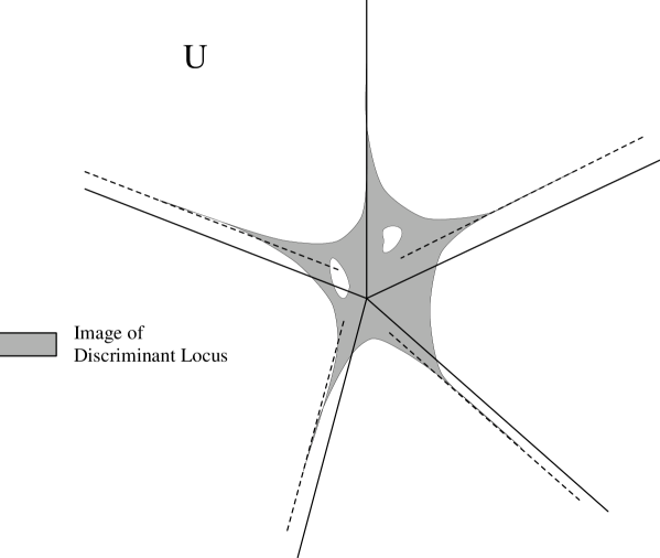
Figure 2: The image the discriminant locus in $U$.

We have now arrived at the “phase” structure of the moduli space described in [3, 2]. Each big cone in the secondary fan corresponds to a region of moduli space under the projection $\pi_{U}$. As we move from one region to another there is a singularity that one may encounter given by the discriminant locus. Notice that in the moduli space $\;\overline{\phantom{X}}$M, one has to aim correctly to hit this singularity — the discriminant locus in $\;\overline{\phantom{X}}$M is complex codimension one and hence may be avoided.

3.2 Compactification of the Moduli Space

The fan structure in $U$ may now be used to specify a compactification $\;\overline{\phantom{X}}$M of M by the usual methods of toric geometry. This, as we will now describe, adds in points in the moduli space associated with points at infinity in $U$.

First we need to give a lattice structure to $U$, i.e., to specify a module ${\mathchoice{\mbox{\bbbfont Z}}{\mbox{\bbbfont Z}}{\mbox{\smallbbbfont Z}}{\mbox{\tinybbbfont Z}}}^{5}$ within the vector space ${\mathchoice{\mbox{\bbbfont R}}{\mbox{\bbbfont R}}{\mbox{\smallbbbfont R}}{\mbox{\tinybbbfont R}}}^{5}$. We use our coordinates $u_{l}$ specify this structure, leading to the lattice points being those with integer coefficients $u_{l}\in{\mathchoice{\mbox{\bbbfont Z}}{\mbox{\bbbfont Z}}{\mbox{\smallbbbfont Z}}{\mbox{\tinybbbfont Z}}}$ for $l=1,\ldots,5$. Consider now each one-dimensional ray $\chi$ in our fan in $U$ and associate to it the lattice point it passes through which is closest to $O$. Call this point $(p_{1}(\chi),p_{2}(\chi),\ldots,p_{5}(\chi))$. In our example each big cone in the secondary fan is a so-called simplicial cone which simply means that it is subtended by 5 rays $\chi_{1},\ldots,\chi_{5}$. For each big cone let us introduce a set of coordinates $(z_{1},z_{2},\ldots,z_{5})$ related to the coordinates $\tilde{a}_{l}$ of $({\mathchoice{\mbox{\bbbfont C}}{\mbox{\bbbfont C}}{\mbox{\smallbbbfont C}}{\mbox{\tinybbbfont C}}}^{*})^{5}$ by

 

$${z_{1}^{p_{1}(\chi_{1})}z_{2}^{p_{1}(\chi_{2})}\ldots z_{5}^{p_{1}(\chi_{5})}}$$

  (26)

If the $z_{l}$’s are all nonzero, they can be taken as coordinates in another $({\mathchoice{\mbox{\bbbfont C}}{\mbox{\bbbfont C}}{\mbox{\smallbbbfont C}}{\mbox{\tinybbbfont C}}}^{*})^{5}$, and (26) defines a map $({\mathchoice{\mbox{\bbbfont C}}{\mbox{\bbbfont C}}{\mbox{\smallbbbfont C}}{\mbox{\tinybbbfont C}}}^{*})^{5}\to({\mathchoice{\mbox{\bbbfont C}}{\mbox{\bbbfont C}}{\mbox{\smallbbbfont C}}{\mbox{\tinybbbfont C}}}^{*})^{5}$ which is finite-to-one. (It will be one-to-one if the determinant of the matrix $(\,p_{i}(\chi_{j})\,)$ is $\pm 1$.) We add to M the points given by the vanishing of any number of the $z_{l}$’s, i.e., we extend the $({\mathchoice{\mbox{\bbbfont C}}{\mbox{\bbbfont C}}{\mbox{\smallbbbfont C}}{\mbox{\tinybbbfont C}}}^{*})^{5}$ space given by the $z_{l}$ coordinates to ${\mathchoice{\mbox{\bbbfont C}}{\mbox{\bbbfont C}}{\mbox{\smallbbbfont C}}{\mbox{\tinybbbfont C}}}^{5}$. Thus each big cone provides a partial compactification of M. For each big cone, the points added locally form the structure of coordinate hyperplanes, i.e., 5 hyperplanes intersecting transversely at a point. This point of intersection will be considered the “point at infinity” or “limit point” associated to the big cone.

When we apply the above process for all of the cones in our fan we form a complete compactification of M and this completely specifies our compactified moduli space $\;\overline{\phantom{X}}$M. The points added form a divisor with normal crossings, i.e., a codimension-one subspace in $\;\overline{\phantom{X}}$M whose irreducible components intersect transversely. It should be noted that the compactified moduli space $\;\overline{\phantom{X}}$M formed this way will not, in general, be smooth and is not smooth in our example. While one might wish to resolve the singularities in this space to address questions about monodromy of periods [35], in this paper it will be important to retain the singularities. It would appear therefore, that at least in some ways, $\;\overline{\phantom{X}}$M, and not its resolution, forms the most natural compactification of the moduli space of Kähler forms on $X$.

There is a relationship between the codimension of parts of the compactification set and the dimension of the cones in our fan. To each cone of real dimension $n$ in our fan, we can associate an irreducible (sub)space of the compactification divisor of $\;\overline{\phantom{X}}$M of complex codimension $n$. For example, each big cone describes a point — the “point at infinity” above which is the point $(0,0,\ldots,0)$ in the coordinates $z_{l}$. Each one-dimensional ray in the fan corresponds to an irreducible component of the compactification divisor. Of particular interest in this paper will be the codimension one walls in the fan which give one complex dimensional subspaces within the compactification divisor. The fact that these one dimensional subspaces are compact and toric means that they are rational curves (isomorphic to ${\mathchoice{\mbox{\bbbfont P}}{\mbox{\bbbfont P}}{\mbox{\smallbbbfont P}}{\mbox{\tinybbbfont P}}}^{1}$) in $\;\overline{\phantom{X}}$M.

Now we will describe how to calculate $r_{\xi}\delta_{\xi}$ for each big cone in $U$ following [33]. Firstly we need to associate a triangulation of the set of points A to each big cone. This was described in detail in [2] and we will again review it briefly here. The triangulation will be determined by the choice of a “height function” $\psi$, which to each point $\alpha_{k}\in{\mathchoice{\mbox{\scrfont A}}{\mbox{\scrfont A}}{\mbox{\smallscrfont A}}{\mbox{\tinyscrfont A}}}$, associates a “height” $\psi(\alpha_{k})\in{\mathchoice{\mbox{\bbbfont R}}{\mbox{\bbbfont R}}{\mbox{\smallbbbfont R}}{\mbox{\tinybbbfont R}}}$. As the name suggests one should think of this as providing the extra coordinate for an embedding ${\mathchoice{\mbox{\scrfont A}}{\mbox{\scrfont A}}{\mbox{\smallscrfont A}}{\mbox{\tinyscrfont A}}}\in{\mathchoice{\mbox{\bbbfont R}}{\mbox{\bbbfont R}}{\mbox{\smallbbbfont R}}{\mbox{\tinybbbfont R}}}^{6}$. The space $U$ can then be considered to be the space of “relative heights”. That is, fix the position of $P^{\circ}$ within this ${\mathchoice{\mbox{\bbbfont R}}{\mbox{\bbbfont R}}{\mbox{\smallbbbfont R}}{\mbox{\tinybbbfont R}}}^{6}$ space by, say, fixing the heights of the vertices of $P^{\circ}$ be have height zero and then let the other points vary to fill out a space of relative heights $\cong U$.

Now consider stretching a piece of rubber over these points which are at various heights. If the heights are generic, the shape thus formed specifies a triangulation of A. The flat faces of the shape will be simplicial specifying the simplices in the triangulation. Points not touching the shape, i.e., below the stretched film are not considered in the triangulation. Thus, for example if $\psi(\alpha_{k})$ is negative for all points not vertices of $P^{\circ}$ and zero for the vertices of $P^{\circ}$, then the triangulation consists of just the simplex $P^{\circ}$ itself. By labeling the points in $U$ according to which triangulation they give, one obtains a fan structure with each big cone specifying a triangulation. Cones of lower dimension specify non-generic heights where one is on the borderline between two or more triangulations.

Let us recall that we began by analyzing the principal discriminant and finding that some of the monomials contained in this naturally dominated in some region of moduli space. To each such monomial we associated a big cone in a fan in the space $U$. Now we have associated a triangulation of the point set A to each such cone. Now we can state the algorithm from [33] which directly specifies the monomial from the triangulation:

Each big simplex (i.e., simplex of maximal dimension), $\sigma$, in the triangulation of A can be given a normalized volume, $\mathop{\rm Vol}\nolimits(\sigma)$, proportional to its actual volume. (The constant of proportionality is fixed so that in a maximal, or “complete,” triangulation, all simplices are have $\mathop{\rm Vol}\nolimits(\sigma)=1$.) Using the notation of (25)

 

$${r_{\xi}}$$

  (27)

where $T_{\xi}$ is the triangulation associated the this monomial. The summation in the equation for $\delta_{\xi}$ is taken over the set of $\sigma\in T_{\xi}$ such that $\alpha_{k}$ is a vertex of $\sigma$. The relative signs of $r_{\xi}$ can also be determined by a process given in [33]. These signs will play an important rôle in our analysis and we will give an equivalent method of their calculation later in this paper.

In our example, the polytope $P^{\circ}$ has normalized volume 18 and there are 100 triangulations leading to convex height functions $\psi(\alpha_{k})$. (Actually these give all possible triangulations of the point set A in this case.) Thus, there are 100 monomials in the sum in (25) and 100 big cones in our fan in $U$. As a simple example, the monomial given by the triangulation consisting of one simplex ($P^{\circ}$ itself) we have

$$r_{\xi}\delta_{\xi}=-18^{18}\,a_{5}^{18}a_{6}^{18}a_{7}^{18}a_{8}^{18}a_{9}^{18}.$$ (28)

At the other extreme, there are 5 possible complete triangulations of the set A. One of them has

$$r_{\xi}\delta_{\xi}=a_{0}^{18}a_{1}^{8}a_{2}^{6}a_{3}^{8}a_{4}^{10}a_{5}^{12}a_{6}^{12}a_{7}^{6}a_{8}^{6}a_{9}^{4}.$$ (29)

Intermediate triangulations give terms such as

$$r_{\xi}\delta_{\xi}=1259712\,a_{0}^{15}a_{1}^{15}a_{3}^{10}a_{5}^{13}a_{6}^{13}a_{7}^{8}a_{8}^{13}a_{9}^{3}.$$ (30)

4 Putting coordinates on the moduli space and the definition of size

So far we have built the complete compact space $\;\overline{\phantom{X}}$M which compactifies the space of complexified Kähler forms on $X$ (or equivalently, complex structure moduli of $Y$) in the context of conformal field theory. What we have does not, at first sight, resemble a space of classical Kähler forms however. In this section we will review how the structure of $\;\overline{\phantom{X}}$M is linked to the classical notion of Kähler forms in some limiting sense and then show how this linkage may be continued to all points in the moduli space. In this way we will extend the usual mathematical notion of volume or size from classical to quantum geometry, as discussed in the introduction. We will explicitly do this by defining coordinates on the Kähler moduli space. In essence, the particular continuation of size from geometry to conformal field theory depends upon how we coordinatize the Kähler moduli space. In most contexts we do not place much importance on coordinate choices as we expect all physical conclusions to be independent of the possible choices. This reasoning is, of course, true here, but there is an important distinction. The space upon which we are putting coordinates is a moduli space, i.e. a space of coupling constants for a class of conformal field theory actions. Different choices of coordinates correspond to different ways of representing and parametrizing these quantum systems. Our goal in this paper is to interpret the geometrical content of all of the conformal theories in the enlarged Kähler moduli space. This goal, in turn, will dictate particular ways of representing these theories (via nonlinear sigma models) and particular parametrizations (directly in terms of their complexified Kähler forms and their analytic continuations) — i.e. a particular choice of coordinates on the moduli space. This, we shall argue, is the choice which makes the geometrical interpretation most clear, but it is certainly not unique.

In fact, we will find it useful to introduce two particular coordinate systems on the enlarged Kähler moduli space of $X$ — each of which will give rise to a definition of “size” at every point of the moduli space. For both of these, we will give an implicit definition of length (inferred from an explicit definition of area) such that both of the following hold:

1. The definition of length in each conformal field theory is given in terms of the fundamental data determining the latter, i.e. its two and three point functions.

2. If the underlying conformal theory is smoothly deformed to a large radius Calabi-Yau sigma model, then the conformal field theory definition of length asymptotically approaches the standard geometrical definition of length on the Calabi-Yau space.

It might be worth pointing out here that such definitions of length should not be expected to be modular invariant. For instance, specifying that a circle has radius $R$ in string theory is not a modular invariant notion because the specified radius obviously differs (almost everywhere) from the equivalent radius $\alpha^{\prime}/R$. Even so, we are certainly justified in saying that string theory on a circle imposes a lower bound of $(\alpha^{\prime})^{1/2}$ on the radius — the point being that this is true in a fundamental domain (in the Teichmüller space) for the modular group. Thus, in this case, in order to associate a notion of size to conformal field theories, we are obligated to make a choice of fundamental domain and work within it. As we shall see, toric geometry provides us directly with the moduli space itself rather than the Teichmüller space. We will construct a fundamental domain so that the large radius limit will be an element of it and so we are forming the analog of the $R>(\alpha^{\prime})^{1/2}$ region in the above context.

In practice, each of the definitions of length we introduce will rely on mirror symmetry. Namely, we have complete analytic understanding of the complex structure moduli space of, say, $Y$. Mirror symmetry provides us with an abstract map from this moduli space to that of the enlarged Kähler moduli space of $X$. Different explicit realizations of this map will associate different coordinates and hence definitions of length to the underlying conformal theories in the Kähler moduli space of $X$. The first explicit realization is mathematically the simplest and amounts to extending the “monomial-divisor mirror map” of [27] throughout the moduli space. The same coordinates also naturally arise from the physical approach of [3] from somewhat the opposite point of view. The second explicit realization makes use of the results of [5] which, via the sigma model, provides a direct link between physical observables and classical geometry.

4.1 The monomial divisor mirror map and the algebraic measure

In section 3 we obtained the result that the space $\;\overline{\phantom{X}}$M contained 100 special points which were obtained from the 100 big cones in our fan in $U$. It was shown in [3, 2] that each of these points could be related to some space that modeled $X$ in the following way. First one takes the cone in $U$ associated to the point in $\;\overline{\phantom{X}}$M. Then one takes the triangulation $T_{\xi}$ of A associated to this cone. This triangulation can then be taken as the base of a set of cones forming a fan $\Delta^{+}$ (not to be confused with the original fan in $U$). From $\Delta^{+}$ one builds a toric variety $V_{\Delta^{+}}$ in the same way as we constructed $\;\overline{\phantom{X}}$M from a fan. The target space $X$ can then be interpreted as the critical locus of some function $W$ within this toric variety. When identifying these models the point $\alpha_{0}$ associated to the monomial with coefficient $a_{0}$ in (16) plays a special rôle. Key examples are as follows:

1. When $T_{\xi}$ is a complete triangulation of A one has that $V_{\Delta^{+}}$ is a line bundle of some smooth toric 4-fold $V$. $X$ is then the Calabi-Yau manifold defined by $W=0$ at infinite radius limit.

2. When $T_{\xi}$ is comprised of only the simplex $P^{\circ}$ then $V_{\Delta^{+}}$ is a point. The target space is this point but the quantum field theory includes some massless modes around this point. This is a Landau-Ginzburg orbifold theory.

3. When $T_{\xi}$ omits some points of A but $\alpha_{0}$ is a vertex of every $\sigma\in T_{\xi}$ then $V_{\Delta^{+}}$ has the structure of a line bundle (in a suitable sense) over some singular space $V$. $X$ is again defined by $W=0$ and is still at some infinite radius limit but has quotient singularities.

4. When $T_{\xi}$ has more than one simplex, $\sigma$, but $\alpha_{0}$ is not a vertex of each $\sigma$ then one has some kind of hybrid model where at least part of $X$ is given by a Landau-Ginzburg orbifold theory “fibered” over a manifold of complex dimension one or two.

The reader may be somewhat surprised that we began with a specific manifold $X$ but now that we have analyzed the global structure of the moduli space of Kähler forms on $X$ we have 100 geometric models all equally as valid as $X$. This is because, as emphasized in [1, 3], conformal field theory happily smooths out topological transformations of $X$ so that our moduli space will, if complete, necessarily contain the other types of $X$ that can be reached from the original $X$.

The key example in this case is case 1. This allows us to identify which cone in $U$ corresponds to the $\sigma$-model we began with. In our example there are 5 complete triangulations of A and hence 5 smooth Calabi-Yau manifolds equally valid as starting points for this analysis.

Picking one of these models, we take the coordinates $z_{l}$ in $\;\overline{\phantom{X}}$M from (26) related to the corresponding big cone. In more physical language, a given point in the moduli space corresponds to some abstract conformal field theory. The coordinates $z_{l}$ are chosen so that the complex structure on $Y$ is such that the resulting correlation functions agree with those of the associated conformal field theory. In other words, we deduce the coupling constants for the sigma model action on $Y$ (the coefficients in 16) by “measuring” scattering amplitudes (calculating correlation functions) in the chosen conformal theory. There is no problem in carrying out this procedure since we can calculate three point functions associated with complex structure moduli exactly by using the results of [20, 36]. So much for the complex structure sector of $Y$.

We now state that the complexified Kähler form on $X$ is given asymptotically by the monomial divisor mirror map [27]:

$$B_{l}+iJ_{l}=\frac{1}{2\pi i}\log(\pm z_{l}),$$ (31)

where we have defined some basis, $e_{l}$, of $H^{2}(X,{\mathchoice{\mbox{\bbbfont Z}}{\mbox{\bbbfont Z}}{\mbox{\smallbbbfont Z}}{\mbox{\tinybbbfont Z}}})$, such that

$$B+iJ=\sum_{l}(B_{l}+iJ_{l})e_{l}.$$ (32)

We then define the cycles $C_{l}\in H_{2}(X)$ by

$$\int_{C_{k}}e_{l}=\delta_{kl}.$$ (33)

and regard a choice of $B+iJ$ as a way of specifying areas:

$$\mathop{\rm Area}\nolimits(C_{l})=\mathop{\rm Im}\nolimits\int_{C_{l}}(B+iJ)=\frac{1}{2\pi}\log|z_{l}|.$$ (34)

(In fact, the “complexified areas” $\int_{C_{l}}(B+iJ)$ are also determined by this choice.)

The sign ambiguity of $z_{l}$ in (31) is referred to in [27] and we will fix it later in this paper. The divisors representing $e_{l}$ may also be determined by the monomial-divisor map [27]. Note that the monomial-divisor mirror map is consistent with the invariance of the theory under the transformation $B\to B+x,\;x\in H^{2}(X,{\mathchoice{\mbox{\bbbfont Z}}{\mbox{\bbbfont Z}}{\mbox{\smallbbbfont Z}}{\mbox{\tinybbbfont Z}}})$, and that the origin of our coordinate patch $z_{l}=0$ corresponds to $J_{l}\to\infty$ consistent with this point being the large radius limit of the Calabi-Yau manifold.

This is our first definition of coordinates. We have constructed the complete moduli space $\;\overline{\phantom{X}}$M of Kähler forms on $X$ and put coordinates on this space that allows us to explicitly assign an area to $2$-cycles at every point in $\;\overline{\phantom{X}}$M. We may consider that the measurement of areas on $X$ is defined by the choice of cohomology class (31), and that this definition agrees with classical geometry at large radii. This definition, as discussed above, can be phrased in terms of the correlation function data of the underlying conformal theory. Therefore, this definition satisfies the two properties emphasized in the beginning of section 4. The measurement of areas defined in this way will be called “the algebraic measure”. This object (or rather, it’s imaginary part) may be used in the same way as the classical Kähler class $J$ to measure the areas on Riemann surfaces in $X$. (In this case, one can also measure the volume of $X$ itself using $J\wedge J\wedge J$, and the volumes of divisors on $X$ using $J\wedge J$, but we will concentrate on the area measurements, for reasons we will see shortly.)

The classical geometric significance of these coordinates is most directly gleaned from the work of [3]. As we have discussed earlier and will explain more fully in [38], Witten’s approach is the physical manifestation of the toric methods under discussion via the relationship between holomorphic and symplectic quotients. The real part of the coordinates $t$ (more generally, $t_{i}$) which appear in the action (7) are, in fact, precisely the algebraic coordinates just defined. That is, if one wants to connect the algebraic measure to some classical notion of distance then the algebraic measure may be thought of as arising from the classical Kähler form on the target space of the non-conformal field theory given by (7).

With this definition of the complexified Kähler class $B+iJ$, the image of the $\sigma$-model phase under the projection $\pi_{U}$ is precisely the Kähler cone of $X$. If one follows a path in $\;\overline{\phantom{X}}$M which moves from the large radius $\sigma$-model on $X$ to a point $m\in{\hbox to0.0pt{$\;\overline{\phantom{X}}$}{\mathchoice{\mbox{\scrfont M}}{\mbox{\scrfont M}}{\mbox{\smallscrfont M}}{\mbox{\tinyscrfont M}}}}$ where $\pi_{U}(m)$ lies outside that cone, then $J_{l}$ becomes negative for some $l$ just as one passes through the wall of the cone. That is, the area of some Riemann surface on $X$ becomes negative at this point. Thus, the 99 other cones in $U$ can be interpreted as a $\sigma$-model on $X$ where some area is negative. As mentioned in the introduction, in the first case studied in [3] of the mirror of the quintic threefold, $U$ was a line and consisted of just two cones, i.e., two rays in either direction from $O$. When one ray is interpreted as the Kähler cone of the Calabi-Yau manifold one sees that the other region must be interpreted as a manifold whose overall volume is negative and that the Landau-Ginzburg orbifold theory can be thought of as a Calabi-Yau manifold with overall volume equal to $-\infty$. Our situation is similar but now we have 99 limit points where the area of some subspace of $X$ (and perhaps the volume of $X$ itself) is $-\infty$.

Four of these other regions actually have all of the associated areas being positive if we interpret the situation not in terms of $X$ but rather in terms of a topologically different manifold — a flop of $X$ [2]. We emphasize that we have not modified the physics in any way; we have only reinterpreted the conformal field theory in terms of its most natural geometrical model. Some of the other 95 limit points correspond to orbifolds. In this context, the orbifold points in the moduli space of Calabi-Yau manifolds would normally be thought of as limit points where some divisor, the exceptional divisor, has shrunk down to zero volume (the reverse of blowing up). When we use the algebraic measure however we arrive at the different conclusion that the volume of the exceptional divisor is $-\infty$ at the orbifold point. (In terms of areas: every Riemann surface within that exceptional divisor has area $-\infty$.) Actually this shift from 0 to $-\infty$ is a recurring feature of many of the other regions. In each case one would naturally have wanted to interpret the conformal field theory as having some target space in which some part of $X$ has shrunk to zero area, but in each case the area defined by the algebraic measure is $-\infty$. The Landau-Ginzburg orbifold model is the extreme case — here the target space is a point, i.e., the whole of $X$ has shrunk to zero, whereas its algebraic areas are all $-\infty$.

Thus we have seen that the algebraic measure has its advantages and disadvantages. It is easily defined in terms of the natural coordinate charts on $\;\overline{\phantom{X}}$M and it reproduces the Kähler cone of $X$. What one might be uncomfortable with however is the fact that most of the moduli space $\;\overline{\phantom{X}}$M is comprised of $X$’s with negative area subspaces and that this definition has a complicated (and largely only implicit) conformal field theory representation.

4.2 The $\sigma$-model measure

We will now make another attempt at defining “size,” this time trying to model more closely the properties of the classical Kähler form. This is done at the expense of the simplicity of the definition in terms of the natural coordinates on $\;\overline{\phantom{X}}$M.

One can use the action (3) to calculate the 3-point function between (chiral,antichiral)-fields in the resulting quantum field theory. This is best achieved by twisting this $N$=(2,2) superconformal $\sigma$-model into the so-called A-model topological field theory [39, 40]. Each field can be associated to an element of $H_{4}(X)$ and the 3-point functions can in principle be calculated from intersection theory. If to each field $\phi_{l}$ we associate a divisor $D_{l}$, then to leading order in the large radius limit we have

$$\langle\phi_{l}\phi_{m}\phi_{n}\rangle\sim\#(D_{l}\cap D_{m}\cap D_{n}).$$ (35)

(We omit the “#” symbol denoting “degree of intersection” from now on.) These intersection numbers agree with those predicted by the monomial-divisor mirror map [1, 41] as explained above. Beyond this asymptotic form of the 3-point functions at large radius limit we may ask what happens if $X$ is near, rather than at, the large radius limit. In this case one may expand the 3-point function out in terms of an instanton series [42]. The instantons in question are given by holomorphically embedded ${\mathchoice{\mbox{\bbbfont P}}{\mbox{\bbbfont P}}{\mbox{\smallbbbfont P}}{\mbox{\tinybbbfont P}}}^{1}$’s in $X$ and for the exact form of this instanton series one should consult [43] (and the references therein) but it can be stated roughly as

$$\langle\phi_{l}\phi_{m}\phi_{n}\rangle=(D_{l}\cap D_{m}\cap D_{n})+\sum_{\Gamma}\frac{{\bf q}^{\Gamma}}{1-{\bf q}^{\Gamma}}(D_{l}\cap\Gamma)(D_{m}\cap\Gamma)(D_{n}\cap\Gamma),$$ (36)

where $\Gamma$ is a holomorphically embedded ${\mathchoice{\mbox{\bbbfont P}}{\mbox{\bbbfont P}}{\mbox{\smallbbbfont P}}{\mbox{\tinybbbfont P}}}^{1}$ in $X$ and ${\bf q}^{\Gamma}$ is a monomial in the $q_{l}$’s. We define the parameters $q_{l}$ by

$$q_{l}=\exp\{2\pi i(B_{l}+iJ_{l})\},$$ (37)

with $B$ and $J$ coming from (3) so that the resulting 3-point functions appear as power series in the $q_{l}$’s. This leads us to another way of defining areas for a point in $\;\overline{\phantom{X}}$M. That is, we determine the values of $B_{l}+iJ_{l}=\int_{C_{l}}B+iJ$ required to give the correct 3-point functions when these 3-point functions are expressed as an instanton sum, i.e., as a power series in $q_{l}$. We then analytically continue this object over the whole moduli space. We will refer to this definition of area-measurement as “the $\sigma$-model measure”. Note that to perform the analytical continuation of the $\sigma$-model measure over $\;\overline{\phantom{X}}$M we need to make some branch cuts in $\;\overline{\phantom{X}}$M. We claim that there is a natural choice and we specify this choice later.

The reason that we distinguish these two definitions of area-measurement in this paper is because they are, in fact, different. That is, in general, $q_{l}\neq z_{l}$ so we will need to specify which coordinates we are using, in order to specify the measures. From now on we will use the symbol $B+iJ$ to refer to the $\sigma$-model measure only.

Returning to Witten’s approach to the algebraic measure outlined in the previous section we see that when one takes the renormalization group flow limit of the field theory given by (7) to the conformal field theory the algebraic measure must “flow” to the $\sigma$-model measure. After all, (7) is describing a sigma-model.

These definitions of the algebraic measure and the $\sigma$-model measure are, as constructed, in complete agreement at the large radius limit. Thus, with our conventions about $B+iJ$ being the $\sigma$-model measure, we can modify (31) to read

$$B_{l}+iJ_{l}=\frac{1}{2\pi i}\left\{\log(\pm z_{l})+O(z_{1},\dots,z_{5})\right\},$$ (38)

i.e., we expand $\log q_{l}$ as a power series for small $z_{l}$. Actually we have not justified the omission of a constant term in the right-hand-side of (38) and we will return to this point briefly later.

In [5] a good geometrical way of picturing these natural $\sigma$-model coordinates in terms of the mirror theory $Y$ was introduced. If we view $\;\overline{\phantom{X}}$M as the moduli space of complex structures of $Y$ then a natural set of coordinates can be introduced via the Gauß-Manin connection. That is, in the case of 3-folds we introduce the holomorphic 3-form $\Omega$ and a set of 3-cycles $\gamma_{n}$. One can then define

$$B_{l}+iJ_{l}=\frac{\displaystyle\int_{\gamma_{l}}\Omega}{\displaystyle\int_{\gamma_{0}}\Omega},$$ (39)

These coordinates are independent of the normalization of $\Omega$ and will satisfy (38) if $\gamma_{0},\gamma_{l}$ are suitably chosen. See [28] for more information. In [5] the definition of the $\sigma$-model measure via (39) was used directly to obtain the correction terms in (38). That is, certain 3-cycles were found and $\Omega$ was integrated over them. In practice this method will be unsuited to approach the problems addressed in this paper. Instead it was noticed in [5] that these periods satisfied a differential equation and in [29] that one could use these differential equations to find the form of (38) without explicitly constructing the 3-cycles $\gamma_{0},\gamma_{l}$.

There is an important qualitative feature of the local solutions to these differential equations. The cycle $\gamma_{0}$ has the property that $\int_{\gamma_{0}}\Omega$ is regular as a function of the $z_{l}$. Thus, comparing (38) with (39), we find

$$2\pi i\,\int_{\gamma_{l}}\Omega=\log(\pm z_{l})\left(\int_{\gamma_{0}}\Omega\right)+O(z_{1},\dots,z_{5})$$ (40)

which tells us that in addition to the regular solution, there is a solution with a $\log(\pm z_{l})$ type growth for each $l=1,\dots,5$. Moreover, all the other solutions will involve products or powers of these log terms. All of this is discussed in more detail in [35].

It is worthwhile noting that whereas we had no problem in in using the algebraic measure to measure areas and volumes of $X$ and its subspaces in the classical way, the same is not true for the $\sigma$-model measure. For example defining

$$\mathop{\rm Vol}\nolimits(X)=\int_{X}J\wedge J\wedge J,$$ (41)

one would find the value of the volume behaved in an unsatisfactory way as one moved around the moduli space. A better definition would be some object of the form of a correlation function $\langle JJJ\rangle$. Some of the properties of the $\sigma$-model measure are actually quite insidious. In the classical picture the Kähler form lives in the linear vector space $H^{2}(X)$. Although we tried to mimic this in the quantum picture by exercising great care in choosing the $\sigma$-model measure coordinates, the quantum corrected moduli space is not flat and this is reflected in some non-linearity in the structure of the $\sigma$-model measure. This underlies the reason why the ring structure given by the wedge product in $H^{*}(X)$ is not a natural object in $\;\overline{\phantom{X}}$M. We will refer to this issue of non-linearity briefly again later in the paper and we hope to address further questions about this structure in future work. In this paper we will only attempt to use the $\sigma$-model measure to directly measure the area of Riemann surfaces in $X$. We will also use the classical notion that if a manifold has zero volume then any subspace within it is also of zero volume. This is the only sense in which we will measure volumes, as opposed to areas of Riemann surfaces.

5 Evaluating the $\sigma$-model measure

5.1 The Hypergeometric System

In this section we will discuss the system of partial differential equations which allow one to find the natural $\sigma$-model coordinates (39) required for the $\sigma$-model measure. With the notation of section 3, let $\alpha_{k}\in{\mathchoice{\mbox{\scrfont A}}{\mbox{\scrfont A}}{\mbox{\smallscrfont A}}{\mbox{\tinyscrfont A}}}$ have coordinates $(\alpha_{k,1},\alpha_{k,2},\ldots,\alpha_{k,5})$ in ${\mathchoice{\mbox{\bbbfont R}}{\mbox{\bbbfont R}}{\mbox{\smallbbbfont R}}{\mbox{\tinybbbfont R}}}^{5}$. For given values of $\beta_{n}$ consider the following differential operators introduced in [44]:

 

$${Z_{n}}$$

  (42)

where $n=1,\ldots,5$ and $l$ labels a relationship

$$\sum_{k}m_{l,k}\alpha_{k,n}=0,\qquad n=1,\ldots,5.$$ (43)

Now we look for a function $\Phi(a_{0},a_{1},\ldots,a_{9})$ such that

$$Z_{n}\Phi=\Box_{l}\Phi=0,\qquad\forall n,l.$$ (44)

The numbers $\beta_{n}$ specify how $\Phi$ transforms under the $({\mathchoice{\mbox{\bbbfont C}}{\mbox{\bbbfont C}}{\mbox{\smallbbbfont C}}{\mbox{\tinybbbfont C}}}^{*})^{5}$ action $x_{i}\to\lambda_{i}x_{i}$. In [45], it was shown that the periods in (39) satisfy (44) for a certain choice of $\beta_{n}$ which we will now give.

We first need to make a special choice of coordinates on the ${\mathchoice{\mbox{\bbbfont R}}{\mbox{\bbbfont R}}{\mbox{\smallbbbfont R}}{\mbox{\tinybbbfont R}}}^{5}$ space in which the points A live. Remember that the (quasi-)homogeneity of (16) means that these points lie in a hyperplane. Let the coordinates be chosen such that $\alpha_{k,5}=1$ for $k=0,\ldots,9$ and let the coordinates of $\alpha_{0}$ be $(0,0,0,0,1)$. In this basis the values of $\beta_{n}$ required are $\beta_{n}=0$ for $n=1,\ldots,4$ and $\beta_{5}=-1$.

We can now give a general solution to the partial differential equations $Z_{n}\Phi=0$ but first we need to say more about $({\mathchoice{\mbox{\bbbfont C}}{\mbox{\bbbfont C}}{\mbox{\smallbbbfont C}}{\mbox{\tinybbbfont C}}}^{*})^{5}$-invariant coordinates. The $a_{k}$ parameters transform under the $({\mathchoice{\mbox{\bbbfont C}}{\mbox{\bbbfont C}}{\mbox{\smallbbbfont C}}{\mbox{\tinybbbfont C}}}^{*})^{5}$-action by the condition that (16) is invariant. This means that for each condition of the form (43) we may introduce

$$z_{l}=\prod_{k}a_{k}^{m_{l,k}}$$ (45)

which are invariant under the $({\mathchoice{\mbox{\bbbfont C}}{\mbox{\bbbfont C}}{\mbox{\smallbbbfont C}}{\mbox{\tinybbbfont C}}}^{*})^{5}$-action. The fact that we are using the same notation $z_{l}$ for such invariants and the coordinate patches on $\;\overline{\phantom{X}}$M in (26) is not an oversight — they can be considered the same thing as we now discuss.

One of the big cones in our fan in $U$ corresponds to the Landau-Ginzburg orbifold model. We know that the local space around the Landau-Ginzburg orbifold point can be parametrized by $a_{0},\ldots,a_{4}$ and setting $a_{5},\ldots,a_{9}=1$. Calling the coordinates for the Landau-Ginzburg orbifold model $z_{l}^{\rm(LG)}$ we thus see that for $a_{5},\ldots,a_{9}=1$ we can define $z_{l}^{\rm(LG)}=a_{l-1}$. We may remove the $a_{5},\ldots,a_{9}=1$ condition by multiplying $a_{l-1}$ by the necessary powers of $a_{5},\ldots,a_{9}$ required to achieve $({\mathchoice{\mbox{\bbbfont C}}{\mbox{\bbbfont C}}{\mbox{\smallbbbfont C}}{\mbox{\tinybbbfont C}}}^{*})^{5}$ invariance, thus we have

$$z_{1}^{\rm(LG)}=a_{0}a_{5}^{-\frac{1}{3}}a_{6}^{-\frac{1}{3}}a_{7}^{-\frac{1}{6}}a_{8}^{-\frac{1}{9}}a_{9}^{-\frac{1}{18}},z_{2}^{\rm(LG)}=a_{1}a_{7}^{-\frac{1}{2}}a_{9}^{-\frac{1}{2}},\ldots$$ (46)

(Fractional powers appear here because the Landau-Ginzburg orbifold point is at a quotient singularity in $\;\overline{\phantom{X}}$M.)

Actually there is a technical point that should be addressed here. The above form for the Landau-Ginzburg orbifold coordinates reflects the fact that there is a ${\mathchoice{\mbox{\bbbfont Z}}{\mbox{\bbbfont Z}}{\mbox{\smallbbbfont Z}}{\mbox{\tinybbbfont Z}}}_{18}$-quotient singularity at this point in the moduli space. Quotient singularities in one complex dimension are trivial is the sense that they can be removed by a change of coordinates. Our description of $\;\overline{\phantom{X}}$M in terms of toric geometry automatically removes such singularities. The ${\mathchoice{\mbox{\bbbfont Z}}{\mbox{\bbbfont Z}}{\mbox{\smallbbbfont Z}}{\mbox{\tinybbbfont Z}}}_{18}$-quotient singularity in the moduli space is actually only a ${\mathchoice{\mbox{\bbbfont Z}}{\mbox{\bbbfont Z}}{\mbox{\smallbbbfont Z}}{\mbox{\tinybbbfont Z}}}_{6}$-quotient singularity once this process is performed. Thus in the toric description given one should actually use a 3-fold cover of the above coordinates. An alternative is to modify the definition of the coordinates $(p_{1}(\chi),p_{2}(\chi),\ldots,p_{5}(\chi))$ in terms of the rays of the secondary fan. Our original definition was in terms of the first point from $O$ encountered by the ray. It turns out that by taking the third point rather than the first for one of the rays restores the ${\mathchoice{\mbox{\bbbfont Z}}{\mbox{\bbbfont Z}}{\mbox{\smallbbbfont Z}}{\mbox{\tinybbbfont Z}}}_{18}$ singularity. (Actually this also occurs when we construct these rays as vectors from the Gale transform of A  [46].) In what follows we assume that $(p_{1}(\chi),p_{2}(\chi),\ldots,p_{5}(\chi))$ has been rescaled for one of the rays in this way.

We may now use (26) to give $({\mathchoice{\mbox{\bbbfont C}}{\mbox{\bbbfont C}}{\mbox{\smallbbbfont C}}{\mbox{\tinybbbfont C}}}^{*})^{5}$-invariant $z_{l}$ coordinates for each big cone in our fan. Thus for each big cone in the fan we have a set of $z_{l}$ coordinates and a set of conditions (43) given by (45).

It is not difficult to show that the equations $Z_{n}\Phi=0$ have as a general solution

$$\Phi(a_{0},a_{1},\ldots,a_{9})=a_{0}^{-1}f(z_{1},z_{2},\ldots,z_{5}),$$ (47)

where $f$ is an arbitrary function and the $z_{l}$’s are any set of $({\mathchoice{\mbox{\bbbfont C}}{\mbox{\bbbfont C}}{\mbox{\smallbbbfont C}}{\mbox{\tinybbbfont C}}}^{*})^{5}$-invariant coordinates. For each big cone we can now write $\Phi$ in the form (47) and write down the $\Box_{l}\Phi=0$ equations.

Let us choose one of the cones corresponding to the large radius limit of a smooth Calabi-Yau manifold and write these differential equations down. We can specify such a cone by specifying a complete triangulation of A. The complete triangulations of A are unique except for the triangle with vertices $\alpha_{7},\alpha_{8},\alpha_{9}$. We will first concentrate on “resolution 1” from [1] given by

(48)

This model is associated with the monomial (29) in the discriminant. Denoting the resulting coordinate patch in $\;\overline{\phantom{X}}$M by $z_{l}^{(1)}$ we obtain

 

$${z_{1}^{(1)}}$$

  (49)

(Note there are no fractional powers of $a_{k}$ since the large radius limit point of a smooth Calabi-Yau manifold is a regular point in $\;\overline{\phantom{X}}$M, in the example we are considering.) At this point we can also state the sign in (31) and (38). We will discuss this issue further in section 5.3. We may associate an integer $d_{l}$ to each coordinate $z_{l}$ defined as the total degree of the numerator or denominator when expressed in terms of $a_{k}$. (38) then becomes

$$B_{l}+iJ_{l}=\frac{1}{2\pi i}\left\{\log\left((-1)^{d_{l}}z_{l}\right)+O(z_{1},\dots,z_{5})\right\}$$ (50)

Thus, in the present example $(-1)^{d_{l}}=1$ for all $l$. The $\Box_{l}$ operators are

 

$${\Box_{1}}$$

  (51)

We can now write down the differential equations we require $\Box_{l}\Phi=0$ by using (47) and (49). Rather than attack this daunting set of equations head on we will turn our attention to sets of ordinary differential equations contained in this set.

5.2 Rational curves in $\;\overline{\phantom{X}}$M.

The points we are particularly interested in, in this paper, are the 100 points in $\;\overline{\phantom{X}}$M which each are the limit of some geometric model, whether it be smooth Calabi-Yau, orbifold, Landau-Ginzburg orbifold, etc. As mentioned in section 3.2 toric geometry tells us that the codimension one walls between the big cones correspond to rational curves within $\;\overline{\phantom{X}}$M. In fact, each such rational curve contains precisely two of our 100 limit points — the two points given by the big cones which this wall separates. In our example, each big cone in $U$ has 5 codimension one faces, that is, given one of the 100 limit points, there are 5 rational curves in $\;\overline{\phantom{X}}$M passing through this point each of which passes through another limit point. In this way, there are 250 rational curves which form a “web” in $\;\overline{\phantom{X}}$M connecting all of the 100 limit points. This is shown as a polytope in figure 3 where lines represent the rational curves and vertices represent limit points. (Actually this is the secondary polytope [34]). Thus it is easily seen that one may move in $\;\overline{\phantom{X}}$M from any of the limit points to another one by moving along these rational curves.

Figure 3: The web formed by rational curves connecting limit points.

As we will now see, the form of the set of partial differential equations from the previous section becomes particularly straight-forward when restricted to these rational curves. We will illustrate this by an example. Let us consider one of the walls of the cone considered in (48). A neighbouring cone to this one corresponds to “resolution 4” of [1], i.e., another smooth Calabi-Yau manifold this time given by the following triangulation:

(52)

For this big cone we have the following coordinates in $\;\overline{\phantom{X}}$M:

 

$${z_{1}^{(2)}}$$

  (53)

That is,

 

$${z_{1}^{(2)}}$$

  (54)

The transition functions between these two patches given in (54) give us the coordinates for the rational curve connecting these limit points, i.e., put $z_{1}^{(1)}=z_{2}^{(1)}=z_{3}^{(1)}=z_{5}^{(1)}=0$ and use $z=z_{4}^{(1)}$ as the coordinate on the rational curve.

Now let us try to solve $\Box_{l}\Phi=0$ on this rational curve $C$. We are interested in finding the regular solution, and the solution with a $\log(\pm z_{4})$-type growth, since their ratio gives the $\sigma$-model coordinate which does not vanish on $C$. To eliminate the other solutions from consideration, we impose the additional equations

$$\left.z_{n}^{(1)}\frac{\partial\Phi}{\partial z_{n}^{(1)}}\right|_{C}=0,\quad n=1,2,3,5.$$ (55)

The solutions to $\Box_{l}\Phi=0$ with a $\log(\pm z_{n})$-type growth for $n\neq 4$, and those that involve powers or products of log terms, will fail to satisfy one of these new equations; thus, we will be left with just the solutions we want.

Using (55) immediately allows us to expand out $\Box_{4}$ in terms of $z$ alone:

$$\Box_{4}\Phi=\frac{1}{a_{1}a_{2}}\left\{z\frac{\partial}{\partial z}z\frac{\partial}{\partial z}-z\left(z\frac{\partial}{\partial z}z\frac{\partial}{\partial z}\right)\right\}\Phi.$$ (56)

Now if we consider $\Phi$ as a function of $z$ alone then we have reduced the problem to an ordinary differential equation.

5.3 Perestroĭka

Before trying to solve the differential equation (56) we will try to generalize the method we followed in the last section so that we can write down the differential equation for any of the rational curves in $\;\overline{\phantom{X}}$M joining two limit points. To do this we will first look at the difference between the triangulations of A corresponding to the two limit points.

For any $N$, consider $N+2$ points in ${\mathchoice{\mbox{\bbbfont R}}{\mbox{\bbbfont R}}{\mbox{\smallbbbfont R}}{\mbox{\tinybbbfont R}}}^{N}$ such that these points are not contained in an ${\mathchoice{\mbox{\bbbfont R}}{\mbox{\bbbfont R}}{\mbox{\smallbbbfont R}}{\mbox{\tinybbbfont R}}}^{N-1}$ hyperplane. Let the polytope $Q$ be the convex hull of these points (i.e., the polytope of minimal volume containing all the points). It follows [47] that there are precisely two triangulations of this set of points which contain at least the vertices of $Q$. The transition between two such triangulations is called a perestroĭka [33]. We will give several examples of perestroĭka in later sections. The usefulness of the notion of a perestroĭka is that two triangulations of A corresponding to neighbouring cones in our fan differ by a perestroĭka. That is, we can associate a perestroĭka to each of the rational curves in $\;\overline{\phantom{X}}$M we are considering.

Denoting the $N+2$ points by $\alpha_{s}$, $s=1,\ldots,N+2$, there will be a single linear relation between these points

$$\sum_{s}m_{s}\vec{\alpha}_{s}=0,$$ (57)

where $\vec{\alpha}_{s}$ is the position vector of $\alpha_{s}$ and the $m_{s}$’s are relatively prime integers. From this relation we define a variable

$$z=\prod_{s}a_{s}^{m_{s}},$$ (58)

and a differential operator

$$\Box=\prod_{m_{s}>0}\left(\frac{\partial}{\partial a_{s}}\right)^{m_{s}}-\prod_{m_{s}<0}\left(\frac{\partial}{\partial a_{s}}\right)^{-m_{s}}.$$ (59)

Setting

$$\Phi(a_{0},a_{1},\ldots)=a_{0}^{-1}f(z),$$ (60)

one can now write $\Box\Phi=0$ as an ordinary differential equation with $z$ as the only dependent variable.

We claim this construction generalizes that of the previous section. That is, for any rational curve joining two limit points in $\;\overline{\phantom{X}}$M we can obtain an ordinary differential equation for the periods on $X$ in terms of $z$, the coordinate on the rational curve. Note that this ordinary differential equation will always be of hypergeometric type.

The hypergeometric ordinary differential equations in question on ${\mathchoice{\mbox{\bbbfont P}}{\mbox{\bbbfont P}}{\mbox{\smallbbbfont P}}{\mbox{\tinybbbfont P}}}^{1}$ has solutions with possible singularities or branch points at three points which we will call $z=0,1,\infty$. The points 0 and $\infty$ are the two limit points which the rational curve connects in $\;\overline{\phantom{X}}$M. $z=1$ is the only other singular point and is thus where the discriminant locus of section 3.2 cuts this curve. To be more precise it is usually the case that the whole rational curve is contained in the discriminant locus. In this case $z=1$ is the point where another irreducible component of the discriminant locus cuts this curve. Given this form of distinguished points on this curve we can now specify our choice of branch cuts to perform any analytic continuation. Each of the points $z=0$ and $z=\infty$ are taken to represent some limit point around which correlation functions may be expanded in some power series. This power series fails when one reaches $z=1$. We thus cut from $z=0$ to $z=1$ and from $z=\infty$ to $z=1$ to reflect this structure. (Any other choice would be artificially unsymmetric.) We extend these cuts from the rational curves on the boundary into the interior of the moduli space, to form a fundamental domain. This choice of fundamental domain is implicit in all that follows in this paper.

In order to put the singularities at $z=1$ we will need to rescale the $z_{l}$’s introduced earlier. The sign of this rescaling is the source of the $(-1)^{d_{l}}$ factors in the monomial-divisor mirror map. We may think of this sign as arising from attempting to fix the mirror map so that the number of lines on a Calabi-Yau manifold is positive. As mentioned earlier, a three-point function in our conformal field theory may be expanded as an instanton sum in $q_{l}$ where the coefficients in this series give information regarding the numbers of holomorphically embedded ${\mathchoice{\mbox{\bbbfont P}}{\mbox{\bbbfont P}}{\mbox{\smallbbbfont P}}{\mbox{\tinybbbfont P}}}^{1}$’s on $X$. In particular the sub-leading term is expected to be the number of lines (that is, the number of holomorphically embedded ${\mathchoice{\mbox{\bbbfont P}}{\mbox{\bbbfont P}}{\mbox{\smallbbbfont P}}{\mbox{\tinybbbfont P}}}^{1}$’s in $X$ the homology class of whose image is some fixed integral generator of $H_{2}(X,{\mathchoice{\mbox{\bbbfont Z}}{\mbox{\bbbfont Z}}{\mbox{\smallbbbfont Z}}{\mbox{\tinybbbfont Z}}})$). To be more precise, in some cases one may have families of lines depending on parameters, and then the “number of lines” must be interpreted by means of the top Chern class of the parameter space of the family [48, 43]. It is generally believed [49, 50] that in such a case a deformation of complex structure to a generic almost complex structure will yield a discrete set of lines. However, some of these lines may count negatively and thus we cannot use this strategy to fix the sign of $z$ in the monomial-divisor mirror map in all cases. Instead, we first note that if there were a three-point function whose expansion in $q_{l}$ had all coefficients positive, then any pole at the edge of convergence of such a series would occur when $q_{l}$ is real and positive. Since $q_{l}=\pm z_{l}$ to leading order, we find the sign required in such a case once we know how to rescale $z_{l}$ to give a pole at $z=1$. This is the sign choice $(-1)^{d_{l}}$ that we specified earlier. By looking at perestroĭka such that one limit point corresponds to a large radius limit smooth Calabi-Yau manifold, one can show that this sign choice is consistent with the signs in the principal discriminant given by [33]. Unfortunately for a general three-point function, not all of the coefficients in the $q_{l}$-expansion need be positive. To maintain consistency with [33] we thus conjecture that the sign given by $(-1)^{d_{l}}$ is always the correct choice even when negative coefficients in the expansion occur. That is, we assume that the pole in the $q_{l}$-expansion of any 3-point function occurs for a real and positive $q_{l}$ (i.e., $B_{l}=0$). If our conjecture is wrong and we were to pick the wrong sign for $z_{l}$ then we would be counting the number of lines on $X$ with the wrong sign.

In summary we thus do the following. Given the definition of $z_{l}$ in (45) we find the constant by which we need to rescale $z_{l}\to z$ to put a pole at $z=1$. The sign of this factor is $(-1)^{d_{l}}$. This sign is absorbed in the monomial-divisor mirror map so that we only take the absolute value of this scale factor in our definition of $z$. Now we will apply this construction to several examples.

It is important to note that although we are describing the following examples from the perspective of our five-parameter example, in each case we only actually study the part of the toric fan specific to the transformation we look at. Thus the following results are clearly valid for any Calabi-Yau moduli space that is studied this way. In fact, in string theory, we expect results concerning flops, blowing-up orbifolds etc., to be dependent only on the local geometry of $X$. This means that the following examples should not be considered dependent on the global structure of $X$.

5.4 The flop

Recall that a flop is the transformation of a manifold into a (possibly) topologically different manifold which replaces a ${\mathchoice{\mbox{\bbbfont P}}{\mbox{\bbbfont P}}{\mbox{\smallbbbfont P}}{\mbox{\tinybbbfont P}}}^{1}$ with another ${\mathchoice{\mbox{\bbbfont P}}{\mbox{\bbbfont P}}{\mbox{\smallbbbfont P}}{\mbox{\tinybbbfont P}}}^{1}$. This occurs by blowing down a ${\mathchoice{\mbox{\bbbfont P}}{\mbox{\bbbfont P}}{\mbox{\smallbbbfont P}}{\mbox{\tinybbbfont P}}}^{1}$ in the original manifold to form a singular space with a double point. This double point can then be resolved by blowing up to give a ${\mathchoice{\mbox{\bbbfont P}}{\mbox{\bbbfont P}}{\mbox{\smallbbbfont P}}{\mbox{\tinybbbfont P}}}^{1}$ in two different ways. One way returns the original manifold and the other way yields another manifold. In general a flop need not take a Kähler manifold to another Kähler manifold. In this paper however we are moving from one manifold to another directly by a change of Kähler form and so in this context we are guaranteed a Kähler flop. Any manifold which was a non-Kähler flop of $X$ would not have a big cone in the secondary fan.

The following perestroĭka is a flop.

(61)

This was precisely the perestroĭka considered in section 5.2. That is, we may specify it by the linear relation (using the numbering conventions of our example)

$$\vec{\alpha}_{3}+\vec{\alpha}_{4}-\vec{\alpha}_{1}-\vec{\alpha}_{2}=0.$$ (62)

The ODE associated the the flop, as we saw (in this case no rescaling of the $z$ parameter is required), is

$$\left(z\frac{d}{dz}\right)^{2}f-z\left(z\frac{d}{dz}\right)^{2}f=0.$$ (63)

This has a general global solution

$$f=C_{1}+C_{2}\log(z),$$ (64)

which is also a general local solution for each $z\neq 1$. We can now follow [29] in finding the $\sigma$-model measure in terms of $z$. The component of the $\sigma$-model measure we find is, of course, the part that varies as we move along the rational curve in $\;\overline{\phantom{X}}$M. To find this Kähler form, we take the solution for $f(z)$ that behaves to leading order like $\log(z)$ at $z=0$ and divide it by the solution which is $2\pi i$ to leading order at $z=0$. That is, we find $B+iJ$ as the ratio of two solutions such that equation (38) is obeyed. In this case this is a trivial task since we have solutions which are exactly a constant and exactly $\log(z)$. Therefore

$$B+iJ=\frac{1}{2\pi i}\log(z).$$ (65)

That is, the $\sigma$-model measure is the same as the algebraic measure. To be more precise when one performs a flop of one Calabi-Yau manifold into another and holds all the other components of the Kähler form at large radius limit then the $\sigma$-model measure coincides with the algebraic measure. In particular, this implies that the area of the flopped ${\mathchoice{\mbox{\bbbfont P}}{\mbox{\bbbfont P}}{\mbox{\smallbbbfont P}}{\mbox{\tinybbbfont P}}}^{1}$ does attain the value zero in the $\sigma$-model definition, just as it does in the algebraic definition. In this setting, therefore, string theory does not supply us with a nonzero lower bound. Of course, the size of the whole manifold is being kept infinite (i.e., any Riemann surface in a class other than the one being flopped has infinite area) and it is only a part of the space which shrinks to zero.

The flop is a bit too trivial to show the full singularity structure in the differential equation. One will find however that many three-point functions will have a pole at $B+iJ=0$.

The fact that the algebraic measure and the $\sigma$-model measure coincide in the region of $\;\overline{\phantom{X}}$M considered in this section has some interesting consequences for the 3-point functions of the superconformal field theory (which we developed in discussions with Witten [3]). It is known [7] that in classical geometry, the Kähler cones of two manifolds related by a flop fit together in ${\mathchoice{\mbox{\bbbfont R}}{\mbox{\bbbfont R}}{\mbox{\smallbbbfont R}}{\mbox{\tinybbbfont R}}}^{h^{1,1}}$ by touching each other along the wall of each Kähler cone (where the area of the flopped ${\mathchoice{\mbox{\bbbfont P}}{\mbox{\bbbfont P}}{\mbox{\smallbbbfont P}}{\mbox{\tinybbbfont P}}}^{1}$ becomes zero). This is equivalent to saying that, so far as Kähler form data is concerned, the class represented by the flopped ${\mathchoice{\mbox{\bbbfont P}}{\mbox{\bbbfont P}}{\mbox{\smallbbbfont P}}{\mbox{\tinybbbfont P}}}^{1}$ has negative area in the flopped manifold. Since the algebraic measure generates the same cone structure as the classical Kähler form, the same considerations must also work for the algebraic measure and thus also for the $\sigma$-model measure.

It is important to bear in mind that the homology class of the ${\mathchoice{\mbox{\bbbfont P}}{\mbox{\bbbfont P}}{\mbox{\smallbbbfont P}}{\mbox{\tinybbbfont P}}}^{1}$ present after the flop is the negative of the homology class present before the flop. Thus, although the class of the original ${\mathchoice{\mbox{\bbbfont P}}{\mbox{\bbbfont P}}{\mbox{\smallbbbfont P}}{\mbox{\tinybbbfont P}}}^{1}$ acquires a negative area as the wall between cones is traversed, the post-flop ${\mathchoice{\mbox{\bbbfont P}}{\mbox{\bbbfont P}}{\mbox{\smallbbbfont P}}{\mbox{\tinybbbfont P}}}^{1}$ will have a positive area in the new region (since it belongs to the opposite class).

In the portion of $\;\overline{\phantom{X}}$M we consider, all Riemann surfaces in $X$, except for the ones being flopped, are of infinite area. Call the finite set of ${\mathchoice{\mbox{\bbbfont P}}{\mbox{\bbbfont P}}{\mbox{\smallbbbfont P}}{\mbox{\tinybbbfont P}}}^{1}$’s being flopped $C_{\beta}$. (These are all in the same homology class.) A 3-point function is then given by

$$\langle\phi_{1}\phi_{2}\phi_{3}\rangle=(D_{1}\cap D_{2}\cap D_{3})+\sum_{\beta}\frac{q}{1-q}(D_{1}\cap C_{\beta})(D_{2}\cap C_{\beta})(D_{3}\cap C_{\beta}),$$ (66)

where $q=\exp\{2\pi i(B+iJ)\}$ and $D_{n}$ is a divisor representing the field $\phi_{n}$ in the usual way.

Let us consider the Calabi-Yau manifold $X_{1}$ at large radius limit. In this limit $q\to 0$ and so the sum in (66) vanishes. Let us now flop $X_{1}$ along the $C_{\beta}$’s to obtain the large radius Calabi-Yau manifold $X_{2}$. Given the discussion above, this is equivalent to sending $J\to-\infty$, i.e., $q\to\infty$. We can take the proper transform of the divisors $D_{n}$ in $X_{1}$ to obtain divisors in $X_{2}$ which we denote by the same symbol. The fundamental equation which relates the intersection numbers before and after the flop is:

$$(D_{1}\cap D_{2}\cap D_{3})_{2}=(D_{1}\cap D_{2}\cap D_{3})_{1}-\sum_{\beta}(D_{1}\cap C_{\beta})_{1}\,(D_{2}\cap C_{\beta})_{1}\,(D_{3}\cap C_{\beta})_{1},$$ (67)

where the subscripts denote in which manifold the intersection numbers are calculated. (Note that $C_{\beta}$ is on $X_{1}$; we will denote the post-flop ${\mathchoice{\mbox{\bbbfont P}}{\mbox{\bbbfont P}}{\mbox{\smallbbbfont P}}{\mbox{\tinybbbfont P}}}^{1}$’s by $C_{\beta}^{\prime}$.) Equation (67) is a statement in classical geometry which is straightforward to verify. For example, if we assume that $D_{1}$ meets $C_{\beta}$ transversely at $k$ points, while $D_{2}$ and $D_{3}$ contain $C_{\beta}$ with multiplicities $l$ and $m$, then $(D_{1}\cap D_{2}\cap D_{3})_{1}=klm$ while $(D_{1}\cap C_{\beta})_{1}=k$, $(D_{2}\cap C_{\beta})_{1}=-l$, and $(D_{3}\cap C_{\beta})_{1}=-m$. On the other hand, after flopping (see figure 4), $D_{2}$ and $D_{3}$ are disjoint (at least locally near $C_{\beta}^{\prime}$) so that $(D_{1}\cap D_{2}\cap D_{3})_{2}=0$, verifying (67) in this case.

Figure 4: A flop.

If we now calculate the 3-point function (66) using (67), we find

 

$${\langle\phi_{1}\phi_{2}\phi_{3}\rangle_{1}}$$

  (68)

where we have used $(D\cap C_{\beta})_{1}=(-D\cap C_{\beta}^{\prime})_{2}$. Noting that the change in sign of homology class $[C_{\beta}^{\prime}]=-[C_{\beta}]$ demands that we replace $q$ by $q^{-1}$, we conclude that $\langle\phi_{1}\phi_{2}\phi_{3}\rangle_{1}=\langle\phi_{1}\phi_{2}\phi_{3}\rangle_{2}$, as expected.

5.5 The $\hbox{\bigbbbfont Z}_{2}$-quotient singularity

The following is the only perestroĭka in one-dimension:

(69)

In this picture the network on the left has 2 lines whereas on the right the middle point is ignored and there is only one line. In our example we have a few such configurations, e.g.,

$$\vec{\alpha}_{3}+\vec{\alpha}_{8}-2\vec{\alpha}_{2}=0.$$ (70)

Indeed this perestroĭka can be applied to (48) by removing the point $\alpha_{2}$ from the triangulation. The model of $X$ thus obtained has a curve of ${\mathchoice{\mbox{\bbbfont Z}}{\mbox{\bbbfont Z}}{\mbox{\smallbbbfont Z}}{\mbox{\tinybbbfont Z}}}_{2}$ quotient singularities [2]. The operation (69) is (moving from right to left) precisely the resolution of a ${\mathchoice{\mbox{\bbbfont Z}}{\mbox{\bbbfont Z}}{\mbox{\smallbbbfont Z}}{\mbox{\tinybbbfont Z}}}_{2}$ quotient singularity in ${\mathchoice{\mbox{\bbbfont C}}{\mbox{\bbbfont C}}{\mbox{\smallbbbfont C}}{\mbox{\tinybbbfont C}}}^{2}$ where the ${\mathchoice{\mbox{\bbbfont Z}}{\mbox{\bbbfont Z}}{\mbox{\smallbbbfont Z}}{\mbox{\tinybbbfont Z}}}_{2}$ action in ${\mathchoice{\mbox{\bbbfont C}}{\mbox{\bbbfont C}}{\mbox{\smallbbbfont C}}{\mbox{\tinybbbfont C}}}^{2}$ is $(z_{1},z_{2})\mapsto(-z_{1},-z_{2})$.

The rational curve associated to the perestroĭka (69) thus joins a limit point of a space with a ${\mathchoice{\mbox{\bbbfont Z}}{\mbox{\bbbfont Z}}{\mbox{\smallbbbfont Z}}{\mbox{\tinybbbfont Z}}}_{2}$ quotient singularity to the limit point of a space where such a singularity has been blown-up (to infinite size).

To put a branch-point at $z=1$ we define

$$z=4\frac{a_{3}a_{8}}{a_{2}^{2}},$$ (71)

i.e., we have introduced a factor of 4. The associated ODE is

$$\left(z\frac{d}{dz}\right)^{2}f-z\left(z\frac{d}{dz}\right)\left(z\frac{d}{dz}+{\textstyle\frac{1}{2}}\right)f=0.$$ (72)

This has a general solution

$$f=C_{1}+C_{2}\log\left(\frac{2-z-2\sqrt{1-z}}{z}\right).$$ (73)

Clearly the term which is constant at $z=0$ is again exactly constant. Expanding the second term around $z=0$ we obtain (assuming the square root to be positive)

$$\log\left(\frac{2-z-2\sqrt{1-z}}{z}\right)=\log(z/4)+{{\textstyle\frac{1}{2}}}z+{{\textstyle\frac{3}{16}}}z^{2}+{{\textstyle\frac{5}{48}}}z^{3}+{{\textstyle\frac{35}{512}}}z^{4}+{{\textstyle\frac{63}{1280}}}z^{5}+O\left(z^{6}\right).$$ (74)

Because of our rescaling of the $z$ variable we now need to look for a solution which behaves like $\log(z/4)$ to leading order. This is simply given by (74). Thus we obtain

$$B+iJ=\frac{1}{2\pi i}\log\left(\frac{2-z-2\sqrt{1-z}}{z}\right).$$ (75)

This therefore gives an example where the $\sigma$-model measure and the algebraic measure do not agree. An interesting question we can ask is what is the value of $B+iJ$ at the orbifold limit point, i.e., when $z\to\infty$. The component of the Kähler form we are studying is the class controlling the areas of Riemann surfaces which lie in the exceptional divisor resulting from blowing-up this singularity. That means that in some sense we are looking at the volume of this exceptional divisor. Naïvely of course from classical geometry we assume that this volume is zero at the orbifold point but we see that the algebraic measure would have us believe that the relevant areas are $-\infty$. To find what the $\sigma$-model measure tells us let us introduce the variable

$$\psi=z^{-1/2}$$ (76)

and then carefully rewrite $B+iJ$ in this variable assuming $0<\arg(\psi)<\pi$ to obtain

$$B+iJ=-\frac{1}{\pi}\cos^{-1}\psi,$$ (77)

where we take the branch corresponding to $\cos^{-1}\psi=\frac{\pi}{2}-\psi+O(\psi^{3})$. (This is consistent with our earlier choice of branch cuts.) Thus we see that the orbifold, given by $\psi=0$ corresponds to $B=-1/2$ and $J=0$. The fact that $J=0$ means that the $\sigma$-model measure agrees with the classical volume, i.e., the volume of the exceptional divisor (and thus the areas of the Riemann surfaces within it) before you blow-up a singularity is zero. More curious is the value $B=-1/2$ at the orbifold point which would appear to have no classical explanation.

Note that we have measured the volume of the exceptional divisor at the the limit point of the orbifold in $\;\overline{\phantom{X}}$M, that is, all sizes except that associated with the exceptional divisor are infinite. It is an interesting question to see whether the exceptional divisor has non-zero volume in the case of an orbifold not at an otherwise large radius limit. We hope to address this question in future work.

Proponents of a universal “$R\to 1/R$” symmetry in the moduli space of string vacua should take note that in passing from the smooth blown-up Calabi-Yau manifold to the orbifold we have been able to shrink the Riemann surfaces within the exceptional divisor completely down to zero size without being able to identify this with some equivalent large radius model. There is no symmetry between the orbifold points and any other points in the moduli space. Thus it would appear that string theory does not remove all distances less than the Planck scale from a moduli space. Some parts of a target space can become as small as they wish at least so long as the rest of the target space is at large radius limit.

In this example in moving from the algebraic measure to the $\sigma$-model measure we have removed negative areas. That is, $J\geq 0$ for all points on the rational curve in $\;\overline{\phantom{X}}$M. We will discuss this further after looking at some more orbifolds.

The branch-point of the general solution of this hypergeometric equation is at $z=\psi=1$, i.e., $B+iJ=0$. This is where many three-point functions will diverge in the conformal field theory. This shows that the only difference between an orbifold, where string theory is known to be well behaved, and a “bad” conformal theory is the value of the $B$-field since in both cases $J=0$, i.e., the volume of the exceptional divisor is zero.

Let us now look at the form of the discriminant for this ${\mathchoice{\mbox{\bbbfont Z}}{\mbox{\bbbfont Z}}{\mbox{\smallbbbfont Z}}{\mbox{\tinybbbfont Z}}}_{2}$ resolution in the context of our example. The monomial for the large-radius limit resolution is given by (29) and one may derive the monomial in $\Delta_{p}$ corresponding to the neighbouring cone in the secondary fan corresponding to the Calabi-Yau space with a curve of ${\mathchoice{\mbox{\bbbfont Z}}{\mbox{\bbbfont Z}}{\mbox{\smallbbbfont Z}}{\mbox{\tinybbbfont Z}}}_{2}$-quotient singularities as

$$r_{\xi}\delta_{\xi}=-64a_{0}^{18}a_{1}^{8}a_{3}^{11}a_{4}^{10}a_{5}^{12}a_{6}^{12}a_{7}^{6}a_{8}^{9}a_{9}^{4}.$$ (78)

If we assert that the discriminant locus intersects our rational curve in $\;\overline{\phantom{X}}$M at $z=1$ then we see immediately that $\Delta_{p}$ for points in $\;\overline{\phantom{X}}$M near this rational curve is given by

 

$${\Delta_{p}}$$

  (79)

This shows how important terms from $\widetilde{\Delta}_{p}$ are on the rational curves in $\;\overline{\phantom{X}}$M. In this case we derive two terms in $\widetilde{\Delta}_{p}$, i.e., terms in $\Delta_{p}$ which could not be obtained by the methods of section 3.2.

In this paper we will usually use the word “orbifold” to refer to a space whose only singularities are locally of the form of quotient singularities. It is more conventional when talking about conformal field theories to consider an orbifold to be globally of the form of a quotient of a smooth manifold (or conformal field theory). In this case one can determine the massless spectrum of the theory to be composed of fields from the original smooth theory combined with twisted fields from the quotient singularities in the new space. (Massive fields can also appear from group elements with no fixed points.) The specific example of a curve of ${\mathchoice{\mbox{\bbbfont Z}}{\mbox{\bbbfont Z}}{\mbox{\smallbbbfont Z}}{\mbox{\tinybbbfont Z}}}_{2}$-quotient singularities we have considered for $z$ given by (71) cannot be globally written as an orbifold. Despite this fact we claim that we can still relate more conventional conformal field theory ideas to this orbifold as we now argue.

Consider the Landau-Ginzburg orbifold theory given by the minimal triangulation of A given by the simplex $\alpha_{5}\alpha_{6}\alpha_{7}\alpha_{8}\alpha_{9}$. This is an orbifold theory in the conformal field theory sense and thus has a “quantum”-symmetry group [51] isomorphic to the group by which we quotiented the original Landau-Ginzburg model. This ${\mathchoice{\mbox{\bbbfont Z}}{\mbox{\bbbfont Z}}{\mbox{\smallbbbfont Z}}{\mbox{\tinybbbfont Z}}}_{18}$ symmetry is given by $x_{4}\to\exp(2\pi i/18)x_{4}$. The monomial $a_{1}x_{2}^{3}x_{4}^{9}$ transforms as a faithful representation of a ${\mathchoice{\mbox{\bbbfont Z}}{\mbox{\bbbfont Z}}{\mbox{\smallbbbfont Z}}{\mbox{\tinybbbfont Z}}}_{2}$ subgroup of this group. Thus if this monomial is added to the Landau-Ginzburg superpotential we would break the ${\mathchoice{\mbox{\bbbfont Z}}{\mbox{\bbbfont Z}}{\mbox{\smallbbbfont Z}}{\mbox{\tinybbbfont Z}}}_{2}$ symmetry. This is precisely the conformal field theory picture of resolving a ${\mathchoice{\mbox{\bbbfont Z}}{\mbox{\bbbfont Z}}{\mbox{\smallbbbfont Z}}{\mbox{\tinybbbfont Z}}}_{2}$-quotient singularity — we add the twisted marginal operator $a_{1}x_{2}^{3}x_{4}^{9}$ into the action to break the discrete symmetry. In terms of toric geometry this resolution of a singularity in $X$ corresponds to a subdivision of the fan representing $X$ by a star subdivision (see for example [2]). Such a subdivision adds a point in A into the triangulation. By the monomial-divisor mirror map, this point in A is precisely the point that represents the monomial which acts as the twisted marginal operator — i.e., $\alpha_{1}$.

In our example we do not have a global quotient singularity but it is locally of the form of a quotient singularity and thus we expect at least the massless part of the conformal field theory to behave as if it were an orbifold. This is because massless twist fields can be considered to be localized around the fixed points. Thus we claim that for the transition given by (71) the “twisted” marginal operator is the monomial corresponding to the point in A added into the triangulation by the perestroĭka — namely $a_{2}x_{3}^{6}x_{4}^{6}$. Indeed if we follow the approach of [2] to find which superpotential, i.e., which values of $a_{k}$, give the relevant space with a ${\mathchoice{\mbox{\bbbfont Z}}{\mbox{\bbbfont Z}}{\mbox{\smallbbbfont Z}}{\mbox{\tinybbbfont Z}}}_{2}$-quotient singularity we find this consistent with $a_{2}=0$, i.e., this marginal operator switched off.

Take the theory with a quotient singularity and perform a perturbative expansion for small values of $a_{2}$ to blow-up the singularity (much along the lines of [52] for example). Our 3-point functions will be in the form of a power series in $a_{2}$, i.e., $\psi=a_{2}/\sqrt{4a_{3}a_{8}}$ if we write things in a $({\mathchoice{\mbox{\bbbfont C}}{\mbox{\bbbfont C}}{\mbox{\smallbbbfont C}}{\mbox{\tinybbbfont C}}}^{*})^{5}$-invariant way. We know that the discriminant locus occurs at $\psi=1$ and so this marks the boundary of the circle of convergence for such a power series. In particular such a perturbative method cannot reach the smooth target space ($\psi\to\infty$) before breaking down.

This is one way of viewing the “phases” picture of the moduli space [3]. In one region of moduli space containing the orbifold theory we may use perturbation theory in twisted (perhaps only in the local sense) marginal operators to calculate all 3-point functions. This region is neighboured by another region containing the point corresponding to the quotient singularity having been resolved with an exceptional divisor of infinite size. Any 3-point function in this region may be calculated by an expansion in terms of instantons given by ${\mathchoice{\mbox{\bbbfont P}}{\mbox{\bbbfont P}}{\mbox{\smallbbbfont P}}{\mbox{\tinybbbfont P}}}^{1}$’s in the exceptional divisor. On the boundary between these two regions the twisted marginal field’s coefficient becomes too large for the twisted field perturbation theory to converge and on the other hand the exceptional divisor becomes too small for the instanton expansion on ${\mathchoice{\mbox{\bbbfont P}}{\mbox{\bbbfont P}}{\mbox{\smallbbbfont P}}{\mbox{\tinybbbfont P}}}^{1}$’s to converge.

5.6 The $\hbox{\bigbbbfont Z}_{3}$-quotient singularity

Consider the following perestroĭka in ${\mathchoice{\mbox{\bbbfont R}}{\mbox{\bbbfont R}}{\mbox{\smallbbbfont R}}{\mbox{\tinybbbfont R}}}^{2}$:

(80)

A fan based on the these triangles gives the toric description of an isolated ${\mathchoice{\mbox{\bbbfont Z}}{\mbox{\bbbfont Z}}{\mbox{\smallbbbfont Z}}{\mbox{\tinybbbfont Z}}}_{3}$-quotient singularity and its blow-up. The quotient singularity in ${\mathchoice{\mbox{\bbbfont C}}{\mbox{\bbbfont C}}{\mbox{\smallbbbfont C}}{\mbox{\tinybbbfont C}}}^{3}$ is given by the action $(z_{1},z_{2},z_{3})\mapsto(\omega z_{1},\omega z_{2},\omega z_{3})$ where $\omega=\exp(2\pi i/3)$. In our example this perestroĭka can occur based on the following relation

$$\vec{\alpha}_{1}+\vec{\alpha}_{7}+\vec{\alpha}_{8}-3\vec{\alpha}_{4}=0.$$ (81)

One of the smooth models of $X$ (resolution number 5 in [1]) admits this perestroĭka and so one of the big cones neighbouring this cone corresponds to a target space that has acquired a ${\mathchoice{\mbox{\bbbfont Z}}{\mbox{\bbbfont Z}}{\mbox{\smallbbbfont Z}}{\mbox{\tinybbbfont Z}}}_{3}$ quotient singularity.

Defining

$$z=-27\frac{a_{1}a_{7}a_{8}}{a_{4}^{3}},$$ (82)

we obtain the differential equation

$$\left(z\frac{d}{dz}\right)^{3}f-z\left(z\frac{d}{dz}\right)\left(z\frac{d}{dz}+{\textstyle\frac{1}{3}}\right)\left(z\frac{d}{dz}+{\textstyle\frac{2}{3}}\right)f=0.$$ (83)

Again the solution that is regular at $z=0$ is just a constant. This time however the solution that behaves like $\log(z)$ cannot be determined in terms of elementary functions.

To find the required solution of (83) we need to turn to the theory of hypergeometric functions. Indeed, with the exception of the flop and the ${\mathchoice{\mbox{\bbbfont Z}}{\mbox{\bbbfont Z}}{\mbox{\smallbbbfont Z}}{\mbox{\tinybbbfont Z}}}_{2}$-orbifold, all the ODE’s we obtain for a perestroĭka will require hypergeometric function theory to find the $\sigma$-model measure.

Recall [53] that the hypergeometric function ${}_{N+1}F_{N}$ is defined by the infinite series

 

$${{}_{N+1}F_{N}(a_{1},a_{2},\ldots,a_{N+1};\,b_{1},b_{2},}$$

  (84)

where $a_{n},b_{n}$ are complex numbers (not to be confused with any previous use of these symbols). This series converges for $|z|<1$. The following ODE has as a solution $f(z)={}_{N+1}F_{N}(a_{1},\ldots;\,b_{1},\ldots;\,z)$:

 

$${\Biggl{\{}z\frac{d}{dz}\left(z\frac{d}{dz}+b_{1}-1\right)}$$

  (85)

All the differential equations encountered when finding the $\sigma$-model measure are of the form (85). Thus applying hypergeometric theory to our differential equation (83) we obtain the solution $f(z)={}_{3}F_{2}(0,{\textstyle\frac{1}{3}},{\textstyle\frac{2}{3}};\,1,1;\,z)=1$. Hence we recover the solution we already knew.

To find the other solution we require, we substitute

$$g(z)=z\frac{d}{dz}f(z)$$ (86)

into (83). This leads to a lower-order hypergeometric differential equation with solution $g(z)={}_{2}F_{1}({\textstyle\frac{1}{3}},{\textstyle\frac{2}{3}};\,1;\,z)$. Expanding this solution we obtain

 

$${f(z)}$$

  (87)

for some constant, $C$. This clearly provides the other solution we require so that

$$B+iJ=\frac{1}{2\pi i}\left\{\log(z/27)+{\textstyle\frac{2}{9}}z+{\textstyle\frac{5}{81}}z^{2}+{\textstyle\frac{560}{19683}}z^{3}+\ldots\right\}$$ (88)

Now let us determine, as we did for the ${\mathchoice{\mbox{\bbbfont Z}}{\mbox{\bbbfont Z}}{\mbox{\smallbbbfont Z}}{\mbox{\tinybbbfont Z}}}_{2}$ quotient singularity, the areas of the Riemann surfaces within the exceptional divisor when $z\to\infty$. In the case of the ${\mathchoice{\mbox{\bbbfont Z}}{\mbox{\bbbfont Z}}{\mbox{\smallbbbfont Z}}{\mbox{\tinybbbfont Z}}}_{2}$ orbifold we have an exact form for the $\sigma$-model measure and so this determination was straight-forward. In the ${\mathchoice{\mbox{\bbbfont Z}}{\mbox{\bbbfont Z}}{\mbox{\smallbbbfont Z}}{\mbox{\tinybbbfont Z}}}_{3}$ case however we only have a series solution and this clearly diverges as $z\to\infty$. What we require therefore is the analytic continuation of the series in (88). This may be done by solving the hypergeometric differential equation, this time as a series expanded around $z=\infty$ and then match these solutions to the solutions around $z=0$. This is known as the connection problem (see for example [54]). In [5] the connection problem was solved by finding a complete set of periods as a series solution around $z=0,1,\infty$ and then demanding that the transformation between these be symplectic. We shall employ another method which is more straight-forward to apply to a general case.

The connection problem is simple to solve with Barne’s-type integrals when no solutions with logarithmic poles are involved. Consider our function $g(z)$ above represented as a Barne’s-type integral:

$${}_{2}F_{1}({\textstyle\frac{1}{3}},{\textstyle\frac{2}{3}};\,1;\,z)=\frac{1}{2\pi i\Gamma({\textstyle\frac{1}{3}})\Gamma({\textstyle\frac{2}{3}})}\int_{-i\infty}^{+i\infty}\frac{\Gamma(t+{\textstyle\frac{1}{3}})\Gamma(t+{\textstyle\frac{2}{3}})\Gamma(-t)}{\Gamma(t+1)}(-z)^{t}\,dt,$$ (89)

where $|\arg(-z)|<\pi$. The integration path moves to the left around the pole at $t=0$ as shown in figure 5.

Figure 5: The integration path for ${}_{2}F_{1}({\textstyle\frac{1}{3}},{\textstyle\frac{2}{3}};\,1;\,z)$.

The series form of this hypergeometric function is recovered if one completes the integration path into a loop to enclose all the poles to the right of the path. The residues at the non-negative integers form the infinite sum. To find these residues and also to prove many of the following relations in this paper we use

$$\Gamma(x)\Gamma(1-x)=\frac{\pi}{\sin(\pi x)}.$$ (90)

One may also complete the path to the left enclosing the poles at $n-{\textstyle\frac{1}{3}},n-{\textstyle\frac{2}{3}}$, where $n$ is a non-positive integer. This expresses our hypergeometric function as another sum which now converges for $|z|>1$. This new sum is therefore the analytic continuation of the original sum. In fact this new sum is a sum of other hypergeometric functions:

 

$${{}_{2}F_{1}({\textstyle\frac{1}{3}},{\textstyle\frac{2}{3}};\,1;\,z)\simeq\frac{\Gamma({\textstyle\frac{1}{3}})}{\Gamma^{2}({\textstyle\frac{2}{3}})}e^{-\frac{\pi i}{3}}\psi\,}$$

  (91)

where “$\simeq$” denotes analytic continuation and we have introduced $\psi=z^{-1/3}$ such that $0<\arg(\psi)<2\pi/3$. For details see, for example, page 136 of [53].

To analytically continue our definition of $B+iJ$ to the orbifold point we need to multiply (91) by $z^{-1}$ and integrate. Doing this directly would introduce an integration constant which would be undetermined. To answer the question of what the size of the exceptional divisor at the orbifold point is, we need to know this constant. Let us instead naïvely apply this process directly to the integrand in the Barne’s-type integral. This gives the following function:

$$h(z)=\frac{1}{2\pi i\Gamma({\textstyle\frac{1}{3}})\Gamma({\textstyle\frac{2}{3}})}\int_{-i\infty}^{+i\infty}\frac{\Gamma(t+{\textstyle\frac{1}{3}})\Gamma(t+{\textstyle\frac{2}{3}})\Gamma(-t)}{t\Gamma(t+1)}(-z)^{t}\,dt.$$ (92)

Completing this path to the right and writing it as a sum of residues we certainly recover the part of (87) which is a power series in $z$. The subtlety arises because of the double pole we now have at $t=0$. Remember that if $w(t)$ is nonzero and finite at $t=0$ then the residue of $w(t)/t^{2}$ at $t=0$ is $(w^{\prime}(t))_{t=0}$. It follows that

$$h(z)=\log(-z)+\Psi({\textstyle\frac{1}{3}})+\Psi({\textstyle\frac{2}{3}})-2\Psi(1)+{\textstyle\frac{2}{9}}z+{\textstyle\frac{5}{81}}z^{2}+{\textstyle\frac{560}{19683}}z^{3}+\ldots,$$ (93)

where $\Psi(n)$ is the digamma or psi function which is defined as the derivative of $\log\Gamma(n)$. Since (from 8.365.6 of [55])

$$\sum_{k=1}^{n-1}\Psi(k/n)-(n-1)\Psi(1)=-n\log n,$$ (94)

we have

$$h(z)=\log(-\frac{z}{27})+{\textstyle\frac{2}{9}}z+{\textstyle\frac{5}{81}}z^{2}+{\textstyle\frac{560}{19683}}z^{3}+\ldots$$ (95)

Thus

$$B+iJ=\frac{1}{2\pi i}h(z)-{\textstyle\frac{1}{2}}.$$ (96)

We can now analytically continue $B+iJ$ into the $|z|>1$ region by completing the path of the integral in (92) to the left and writing it as a sum over residues. The result is

 

$${h(z)=-3\frac{\Gamma({\textstyle\frac{1}{3}})}{\Gamma^{2}({\textstyle\frac{2}{3}})}e^{-\frac{\pi i}{3}}\psi\,}$$

  (97)

Note this is a combination of hypergeometric functions which are solutions to third-order differential equations. These equations may be derived directly from (83) by suitable changes of variable.

Putting $\psi=0$ to obtain the orbifold point we see that $B+iJ=-{\textstyle\frac{1}{2}}$. Thus the size of the exceptional divisor is again zero and again the $B$-field has value $-{\textstyle\frac{1}{2}}$. Notice the cancellation that was required between the digamma functions appearing from the double pole in the Barne’s-type integral and the $\mathop{\rm Vol}\nolimits(\sigma)^{\mathop{\rm Vol}\nolimits(\sigma)}$-type factors that were required to achieve this seemingly trivial final result.

Note from (97) that, for $|\psi|\ll 1$ we have $\pi/6<\arg({\textstyle\frac{1}{2\pi i}}h(z))<5\pi/6$. This shows that $J\geq 0$, i.e., we have only non-negative areas in this region. In fact, negative areas are completely excluded from the conformal field theories parameterized by this rational curve in $\;\overline{\phantom{X}}$M.

We have also done enough to determine the value of $B+iJ$ at $z=1$ where we expect the conformal field theory to be singular. One finds $B=0$ and $J\approx 0.463$ ($\approx 18.3\alpha^{\prime}$ putting back units of length). Thus, in contrast to the ${\mathchoice{\mbox{\bbbfont Z}}{\mbox{\bbbfont Z}}{\mbox{\smallbbbfont Z}}{\mbox{\tinybbbfont Z}}}_{2}$-singularity case, the discriminant now vanishes when we acquire a specific non-zero size for the exceptional divisor.

Naturally everything we said about the description of a theory in terms of twisted marginal operators in the last section also applies to this case. In our example the twisted marginal operator resolving the ${\mathchoice{\mbox{\bbbfont Z}}{\mbox{\bbbfont Z}}{\mbox{\smallbbbfont Z}}{\mbox{\tinybbbfont Z}}}_{3}$-quotient singularity would be $a_{4}x_{2}^{3}x_{3}^{3}x_{4}^{3}$. Again this is only locally of the form of a quotient singularity and this operator is not twisted under any global symmetry of a covering theory.

The moduli space of Kähler forms on the so-called $Z$-manifold was studied in [56]. This manifold is the resolution of an orbifold with ${\mathchoice{\mbox{\bbbfont Z}}{\mbox{\bbbfont Z}}{\mbox{\smallbbbfont Z}}{\mbox{\tinybbbfont Z}}}_{3}$-quotient singularities of the form studied in this section. Indeed similar hypergeometric functions appear in [56] where the entire region of moduli space in the orbifold “phase” is studied.

5.7 The $\hbox{\bigbbbfont Z}_{4}$-quotient singularity

In this paper we will concentrate mainly on perestroĭka which take one from a large radius limit smooth Calabi-Yau manifold to a neighbouring cone. This is because we know how to define the Kähler form for the smooth Calabi-Yau manifold by using the monomial-divisor mirror map. If we look at any other perestroĭka it would be necessary to first determine $B+iJ$ at one of the limit points by following a path from a smooth Calabi-Yau manifold limit point. As we discuss briefly later, such a path will usually raise considerations about basis changes as one moves from one perestroĭka to the next. In this section we look at a simple example where we may ignore such problems. That is, we will blow down two irreducible divisors which will not “interfere” with each other and thus no basis change is required.

Any quotient singularity in Calabi-Yau spaces of complex dimension 3 other than the two we have just studied will require an exceptional divisor with more than one irreducible component. This means that a complete resolution of the singularity requires more than one perestroĭka. Consider the next simplest case:

(98)

The bottom-right diagram is the toric picture for a ${\mathchoice{\mbox{\bbbfont Z}}{\mbox{\bbbfont Z}}{\mbox{\smallbbbfont Z}}{\mbox{\tinybbbfont Z}}}_{4}$-quotient singularity in ${\mathchoice{\mbox{\bbbfont C}}{\mbox{\bbbfont C}}{\mbox{\smallbbbfont C}}{\mbox{\tinybbbfont C}}}^{3}$ generated by $(z_{1},z_{2},z_{3})\mapsto(iz_{1},iz_{2},-z_{3})$. The top-left diagram is the complete blow-up of this singularity to give a smooth space. There are two irreducible components to the exceptional divisor and thus two perestroĭka are involved. The two components of the exceptional divisor may be produced in either order in the blow-up procedure so that there are two possible paths the perform the blow-up as shown above.

Such a choice of paths is a common feature in $\;\overline{\phantom{X}}$M. It is clear from figure 3 that the journey between any two limit points may be taken along many paths. In order for us to be able to give a value of the $\sigma$-model measure to each limit point we require that the choice of paths does not affect this value.

One of the paths in this ${\mathchoice{\mbox{\bbbfont Z}}{\mbox{\bbbfont Z}}{\mbox{\smallbbbfont Z}}{\mbox{\tinybbbfont Z}}}_{4}$ example (taken along line 2 and 1 in (98)) consists of two perestroĭka of the type considered in section 5.5. We know therefore that this path leads to zero volumes for both components of the exceptional divisor in the orbifold limit. In the alternative path, line 4 is also of this type so that one component of the exceptional divisor is again zero at the orbifold point. In order for (98) to be commutative we thus require that the perestroĭka given by line 3 gives zero volume at this point as we will now check.

In our example this configuration is given by

$$\vec{\alpha}_{3}+2\vec{\alpha}_{7}+\vec{\alpha}_{8}-4\vec{\alpha}_{4}=0,$$ (99)

leading to

$$z=64\frac{a_{3}a_{7}^{2}a_{8}}{a_{4}^{4}}.$$ (100)

We can now follow the procedure in section 5.6 where now we are dealing with the solutions of the equation related to the hypergeometric function ${}_{4}F_{3}(0,{\textstyle\frac{1}{4}},{\textstyle\frac{1}{2}},{\textstyle\frac{3}{4}};\,{\textstyle\frac{1}{2}},1,1;\,z)$. Again the regular solution is a constant and again we obtain the other solution by the trick in equation (92). This time we obtain

 

$${h(z)}$$

  (101)

where $\psi=z^{-1/4}$ and $0<\arg(\psi)<\pi/2$. Thus at the orbifold point, as $\psi\to 0$ we have zero volume again as we expected.

5.8 Changing the dimension of $X$

Thus far we have always obtained the the result that $B+iJ=-{\textstyle\frac{1}{2}}$ at the limit point where we remove a point from A from the triangulation. This is not a general feature. It is not difficult to convince oneself however that it will be when can use the constructions above. That is, the digamma functions introduced by the double pole at $z=0$ will cancel the factor introduced in the definition of $z$. This construction of the $\sigma$-model measure relied on the fact that one of the solutions of the hypergeometric differential equation was a constant.

Remember from (60) that $a_{0}$ plays a distinguished rôle in our hypergeometric system. So far, non of the perestroĭka considered have involved the point $\alpha_{0}$. So long as this is true, we will obtain a hypergeometric equation with a constant solution. In fact, it is not hard to prove that the condition for not having a constant solution is as follows. When the linear relation (57) is formed, $m_{0}$ must be non-zero and have opposite sign to the other non-zero $m_{s}$’s. This statement is equivalent to the statement that the associated perestroĭka consists of removing (or adding) $\alpha_{0}$ to the triangulation.

It was shown in [2] that the point $\alpha_{0}$ plays a distinguished rôle for another reason. If $\alpha_{0}$ is a vertex of every simplex in the triangulation of A then $X$ may be interpreted as an irreducible space of complex dimension 3. If $\alpha_{0}$ is a vertex of only some of the simplices then $X$ is reducible with only part of $X$ having a 3-dimensional representation. If $\alpha_{0}$ does not appear in the triangulation then the dimension of $X$ is $<3$. Thus, the perestroĭka we have not yet considered are the ones which lower the dimension of $X$ down from 3.

An extreme example of this is effectively the one studied in [5] where the other limit point is a Landau-Ginzburg orbifold theory, i.e., $X$ has dimension 0. We shall first study one of the neighbours of “resolution 5” of [1] where the dimension is shrunk down to 2 (see [2] for a full explanation of this). The perestroĭka is identical to that considered in section 5.6 except now the relation is

$$\vec{\alpha}_{4}+\vec{\alpha}_{5}+\vec{\alpha}_{6}-3\vec{\alpha}_{0}=0,$$ (102)

and thus

$$z=-27\frac{a_{4}a_{5}a_{6}}{a_{0}^{3}}.$$ (103)

Now the differential equation is

 

$${\left(z\frac{d}{dz}\right)^{3}f-}$$

  (104)

Thus, the solution which is regular at $z=0$ is given by $f(z)={}_{2}F_{1}({\textstyle\frac{1}{3}},{\textstyle\frac{2}{3}};\,1;\,z)$. In (91) we gave the analytic continuation of this for $|z|>1$. We now need to find the solution of (104) that behaves as $\log(z)$ at $z=0$ and continue this to $|z|>1$.

From our earlier analysis of Barne’s-type integrals we saw that a double pole gave a residue with a $\log(z)$ term. With this success in mind consider the following

$$h(z)=-\frac{1}{2\pi i\Gamma({\textstyle\frac{1}{3}})\Gamma({\textstyle\frac{2}{3}})}\int_{-i\infty}^{+i\infty}\Gamma(t+{\textstyle\frac{1}{3}})\Gamma(t+{\textstyle\frac{2}{3}})\Gamma^{2}(-t)z^{t}\,dt.$$ (105)

Completing the path to the right and taking residues we obtain

 

$${h(z)={}_{2}F_{1}({\textstyle\frac{1}{3}},{\textstyle\frac{2}{3}};\,1;\,z)}$$

  (106)

Completing the path to the left and taking residues we obtain

 

$${h(z)=-\frac{\Gamma({\textstyle\frac{1}{3}})}{\Gamma^{2}({\textstyle\frac{2}{3}})}\frac{\pi}{\sin(\frac{\pi}{3})}}$$

  (107)

where, as in section 5.6, $\psi=z^{-1/3}$ and $0<\arg(\psi)<2\pi/3$. The above expresses $h(z)$ as a linear combination of the same functions that appeared in (91) and so $f(z)=h(z)$ is a solution of (104). Thus we have found the solution that behaves like $\log(z)$ at $z=0$ and its analytic continuation for $|z|>1$. This is a general method for finding the extra solutions of a hypergeometric equation whose regular solution is ${}_{N+1}F_{N}(a_{1},a_{2},\ldots;\,1,1,\ldots;\,z)$ — simply take some of the $\Gamma(t+1)$ factors in the denominator of the Barne’s-type integral and move them into the numerator as $\Gamma(-t)$ terms (with a change in sign of $z$ for each term). This produces a high-order pole at $z=0$ which gives some power of $\log(z)$ when the residue is taken.

The monomial-divisor mirror map tells us

$$B+iJ=\frac{1}{2\pi i}\frac{h(z)}{{}_{2}F_{1}({\textstyle\frac{1}{3}},{\textstyle\frac{2}{3}};\,1;\,z)}.$$ (108)

To find the value of $B+iJ$ at the limit point corresponding to the 2-dimensional target space, we take $|\psi|\ll 1$ whence from (91) and (107) we obtain

$$B+iJ\simeq\frac{ie^{\frac{\pi i}{3}}}{2\sin\frac{\pi}{3}}\left\{1-3\frac{\Gamma^{3}({\textstyle\frac{2}{3}})}{\Gamma^{3}({\textstyle\frac{1}{3}})}(1-e^{-\frac{\pi i}{3}})\psi+O(\psi^{2})\right\}.$$ (109)

Thus for $\psi=0$ we have $B=-{\textstyle\frac{1}{2}}$ and $J={\textstyle\frac{1}{2}}\cot(\pi/3)$. That is, the area of the generator of $H_{2}(X,{\mathchoice{\mbox{\bbbfont Z}}{\mbox{\bbbfont Z}}{\mbox{\smallbbbfont Z}}{\mbox{\tinybbbfont Z}}})$ (and thus we infer the volume of $X$) at this limit point is not zero. We also see from the above expression that for small $\psi$ we have

$$\pi/6<\arg\left((B+iJ)-(B+iJ)_{\psi=0}\right)<5\pi/6,$$ (110)

showing how the size always increases as we move away from $\psi=0$.

The method of calculation we have just done may also be applied to the mirror of the quintic threefold as studied in [5]. In this case we obtain the result that at the Landau-Ginzburg orbifold point we obtain $J={\textstyle\frac{1}{2}}\cot(\pi/5)$ (which is equal to $\frac{4}{5}\sin^{3}(2\pi/5)$ as stated in [5]).

We thus see that it is impossible to shrink the whole Calabi-Yau manifold down to a point as measured by the $\sigma$-model measure. If we think of a path on figure 3 that begins at a smooth Calabi-Yau point and ends on the Landau-Ginzburg orbifold point then one of the lines we traverse must correspond to a perestroĭka that removes $\alpha_{0}$ and hence yields $J>0$. Notice that to calculate the value of $B+iJ$ at, say, the Landau-Ginzburg orbifold point is quite complicated. As we follow a path along the web of figure 3, at each vertex we have to change the basis of $B+iJ$ to prepare for the next perestroĭka. Because, as mentioned, earlier we do not have a nice linear structure on the moduli space expressed in terms of the $\sigma$-model measure coordinates, the basis change will generally involve transcendental functions.

Consider the perestroĭka that adds the point $\alpha_{0}$ to the minimal triangulation comprising of just the simplex $P^{\circ}$. This is the transition between the Landau-Ginzburg orbifold and the Calabi-Yau space which is a hypersurface in the unresolved ${\mathchoice{\mbox{\bbbfont P}}{\mbox{\bbbfont P}}{\mbox{\smallbbbfont P}}{\mbox{\tinybbbfont P}}}^{4}_{\{6,6,3,2,1\}}$ (see [2] for more details). If we measure the volume of the Landau-Ginzburg orbifold according to this transition by the above calculation we obtain $J={\textstyle\frac{1}{2}}\cot(\pi/18)$. This shows that the above value of $J={\textstyle\frac{1}{2}}\cot(\pi/3)$ must change as we blow-down the remaining parts of $X$ to obtain the Landau-Ginzburg orbifold. This change occurs because of the basis changes in this process.

6 Discussion and Conclusion

We began this paper by noting two properties of string theory which are relevant for understanding the space of allowed target space metrics. First, recent work [1, 2, 3] has shown that string theory makes sense even if the target space metric does not satisfy the usual positivity conditions that one classically expects. In this regard we are led to augment the space of allowed Kähler forms beyond the usual Kähler cone. Second, a number of works have demonstrated that string theory appears to impose “minimal lengths” and hence restricts the physically relevant space of Kähler forms to lie within the usual Kähler cone. Part of the purpose of the present work has been to study these divergent tendencies and show that, in fact, they are completely consistent.

In particular, since the concept of “size” is an intrinsically classical mathematical notion, we have carefully studied ways of extending its meaning to the more abstract realm of conformal field theory. In essence, we have sought to find natural continuations of the definition of size from classical to quantum geometry. There is no unique way of doing this. We have found, though, that when our conformal field theory has a sigma model interpretation we can extract a definition of size, by using mirror symmetry, from the geometric structure of the latter. We can then extend this definition by analytic continuation to all theories in the enlarged Kähler moduli space. We have seen, in particular, that this gives rise to a precise meaning, rooted in the structure of conformal sigma models, to the area of two-cycles throughout the moduli space.

With sufficient calculational power, we would explicitly carry out this program and thereby study the full realm of possible areas for these cycles. The work of [1, 2, 3], for example, would appear to indicate that zero and negative areas would necessarily arise. The present paper, though, has shown that the definition of area that one would directly extract from these works (the algebraic measure) does not agree with the natural sigma model Kähler form discussed above. We have therefore sought to determine if the latter definition restores something akin to the usual positivity conditions. For calculational ease, we have limited our attention to particular complex dimension one subspaces in the enlarged Kähler moduli space for the illustrative example studied in [1, 2].

In terms of the algebraic measure the enlarged moduli space of Kähler forms naturally leads to many “Kähler cones”, each associated to its own geometric model of $X$, glued together spanning the whole ${\mathchoice{\mbox{\bbbfont R}}{\mbox{\bbbfont R}}{\mbox{\smallbbbfont R}}{\mbox{\tinybbbfont R}}}^{h^{1,1}}$. In our example there are 100 such cones of which 5 correspond to smooth Calabi-Yau manifolds. We have considered complex dimension one spaces in this moduli space which join the “large radius limit points” in each region. In order to determine the value of the $\sigma$-model measure at each of these limit points, we have considered the network of rational curves in the compactification divisor of the moduli space which connects them. Each such rational curve leads to an ordinary hypergeometric equation allowing for an analysis along the lines of [5]. It is reasonable to expect that the extreme values of the $\sigma$-model measure will occur at the these limit points. In this paper we have demonstrated this only in a limited sense by looking at the neighbourhoods within rational curves of some of the limit points, where we discover that not all values in ${\mathchoice{\mbox{\bbbfont R}}{\mbox{\bbbfont R}}{\mbox{\smallbbbfont R}}{\mbox{\tinybbbfont R}}}^{h^{1,1}}$ are attained by the $\sigma$-model measure. To be more precise, all necessarily negative areas are eliminated as well as small positive sizes where all components of the $\sigma$-model measure are small. Notice however that some Riemann surfaces can be shrunk down to zero area while other parts of $X$ are held at large-radius limit.

More precisely, if we plot the “$J$” part of the $\sigma$-model measure (i.e., the imaginary part of $B+iJ$) in ${\mathchoice{\mbox{\bbbfont R}}{\mbox{\bbbfont R}}{\mbox{\smallbbbfont R}}{\mbox{\tinybbbfont R}}}^{h^{1,1}}$ we do not find a cone structure for each of the 100 phase regions. The 5 cones of the smooth Calabi-Yau models are retained as cones asymptotically away from the origin since the $\sigma$-model measure and the algebraic measure coincide there. All of the other 95 limit points are mapped somewhere within these 5 cones — i.e., they all have non-negative areas with respect to at least one of these 5 models. Thus, assuming these limit points represent extreme values of $J$, the whole moduli space of $\sigma$-model measures maps into this union of 5 cones. We can represent this idea in figure 6. We show roughly how the space of algebraic $J$’s as shown in figure 2 is expected to be modified in going to the same diagram of the $\sigma$-model measure $J$ in a hypothetical example where two of the cones give smooth Calabi-Yau manifolds. The two smooth Calabi-Yau regions are labeled $X_{1}$ and $X_{2}$ and the other regions are labeled a, b and c.

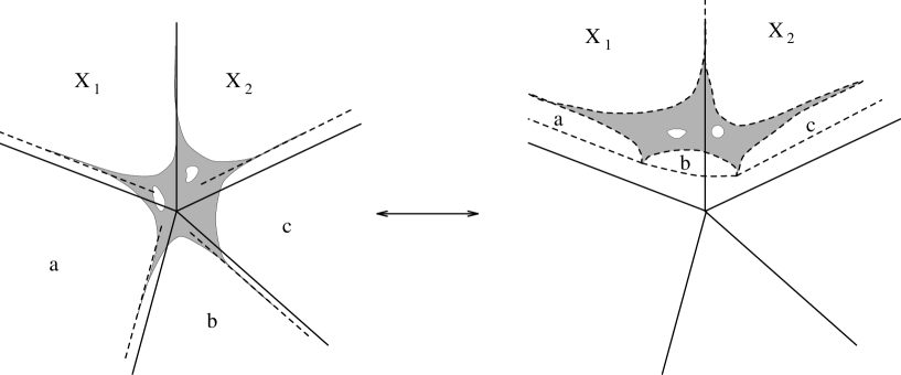
Figure 6: The different phases as they appear in $J$-space for

the algebraic measure (on the left) and the $\sigma$-model measure (on the right).

It would appear therefore that no negative areas appear in the space of conformal field theories describing non-linear $\sigma$-models or at least if negative areas do occur then they can be redefined away by using a topologically different model for $X$. Thus, string theory does require us to enlarge the space of allowed Kähler forms beyond the usual classical Kähler cone, but it does so in a manner consistent with non-negative areas. In this way, we resolve the puzzle discussed at the beginning of this section and in the introduction.

It is interesting to compare the results of this paper with the results of classical general relativity — i.e., the moduli space of Ricci-flat metrics on $X$. It turns out that that both the flop and the quotient singularity (and its blow-up) appear as limiting classical solutions to the Einstein equations. First we describe the flop. This case was studied in [57] and we shall repeat here only an outline of the argument. With a $2\times 2$ matrix representation of the coordinates, $W$, one can define a distance $r^{2}=\mathop{\rm tr}\nolimits(W^{\dagger}W)$ from the double point when the ${\mathchoice{\mbox{\bbbfont P}}{\mbox{\bbbfont P}}{\mbox{\smallbbbfont P}}{\mbox{\tinybbbfont P}}}^{1}$ is blown down. The metric can then be written

$$ds^{2}={\mathchoice{\mbox{\scrfont F}}{\mbox{\scrfont F}}{\mbox{\smallscrfont F}}{\mbox{\tinyscrfont F}}}\,{}^{\prime}\mathop{\rm tr}\nolimits(dW^{\dagger}\,dW)+{\mathchoice{\mbox{\scrfont F}}{\mbox{\scrfont F}}{\mbox{\smallscrfont F}}{\mbox{\tinyscrfont F}}}\,{}^{\prime\prime}\left|\mathop{\rm tr}\nolimits(dW^{\dagger}\,dW)\right|^{2}+4c\frac{|d\lambda|^{2}}{1+|\lambda|^{2}},$$ (111)

where F is some function of $r$ and $\lambda$ is the coordinate on the ${\mathchoice{\mbox{\bbbfont P}}{\mbox{\bbbfont P}}{\mbox{\smallbbbfont P}}{\mbox{\tinybbbfont P}}}^{1}$. The real parameter $c$ in the above corresponds to the area of the flopped ${\mathchoice{\mbox{\bbbfont P}}{\mbox{\bbbfont P}}{\mbox{\smallbbbfont P}}{\mbox{\tinybbbfont P}}}^{1}$ and thus may be taken as the component of the (real) Kähler form which gives this area. If $c=0$ then the above metric is degenerate (in the sense that some distinguished points are now separated by zero distance). If $c<0$ one may change coordinates to give a smooth metric with a ${\mathchoice{\mbox{\bbbfont P}}{\mbox{\bbbfont P}}{\mbox{\smallbbbfont P}}{\mbox{\tinybbbfont P}}}^{1}$ with area $-c$ [57]. Thus we see that the only difference between this picture and the stringy picture we presented in terms of $\;\overline{\phantom{X}}$M is that we have an extra degree of freedom in the $B$-field which may be used to smooth out the singularity at $c=0$ as far the conformal field theory is concerned [1].

When we turn to the quotient singularity there is a bigger difference. For example, let us consider the blow-up of the singularity of the type considered in section 5.6. Near the ${\mathchoice{\mbox{\bbbfont Z}}{\mbox{\bbbfont Z}}{\mbox{\smallbbbfont Z}}{\mbox{\tinybbbfont Z}}}_{3}$ singularity, or its blow-up, we have [58]:

$$ds^{2}=2\frac{(c^{3}+L^{3})^{\frac{1}{3}}}{L}\left\{dx^{i}d\bar{x}^{i}-\frac{c^{3}}{L(c^{3}+L^{3})}\bar{x}^{i}dx^{i}x^{j}d\bar{x}^{j}\right\},$$ (112)

where $L=x^{i}\bar{x}^{i}$. This contains a real parameter $c>0$ for a smooth metric (with suitable change of coordinates). This is roughly the form of the metric irrespective of the global geometry so long as $x,\sqrt{c}\ll R$, where $R$ is some characteristic length of the global geometry of $X$. As shown in [58] this geometry contains a ${\mathchoice{\mbox{\bbbfont P}}{\mbox{\bbbfont P}}{\mbox{\smallbbbfont P}}{\mbox{\tinybbbfont P}}}^{2}$ submanifold with the standard Fubini-Study metric. The line element, $ds^{2}$, on this ${\mathchoice{\mbox{\bbbfont P}}{\mbox{\bbbfont P}}{\mbox{\smallbbbfont P}}{\mbox{\tinybbbfont P}}}^{2}$ is proportional to the parameter $c$. This ${\mathchoice{\mbox{\bbbfont P}}{\mbox{\bbbfont P}}{\mbox{\smallbbbfont P}}{\mbox{\tinybbbfont P}}}^{2}$ is clearly the exceptional divisor with $c=0$ giving the quotient singularity. Varying this parameter thus corresponds to varying the component of the real Kähler form that gives the volume of the exceptional divisor. For a smooth metric we require $c>0$. This gives the classical moduli space a boundary. If we continue into the $c<0$ region then the ${\mathchoice{\mbox{\bbbfont P}}{\mbox{\bbbfont P}}{\mbox{\smallbbbfont P}}{\mbox{\tinybbbfont P}}}^{2}$ acquires negative size and part of $X$ becomes “pinched off”. This metric is still Ricci-flat and so depending on one’s qualms about negative areas one might wish to consider this a solution of classical general relativity.

When we look at the orbifold point in $\;\overline{\phantom{X}}$M we see a different picture. Now the point in $\;\overline{\phantom{X}}$M which corresponds to a zero volume exceptional divisor is not on a boundary — $\;\overline{\phantom{X}}$M has no boundary. As we move in any direction away from this point the volume of the exceptional divisor becomes positive (or remains zero) and so we never need to address the question of negative volumes. We are unable to pinch off regions of space in this manner. In general the singularities in the conformal field theories appear in a different location in the moduli space compared to the classical picture. In the case of a ${\mathchoice{\mbox{\bbbfont Z}}{\mbox{\bbbfont Z}}{\mbox{\smallbbbfont Z}}{\mbox{\tinybbbfont Z}}}_{2}$-quotient singularity the singular theory appears at zero-volume exceptional divisor, i.e., just where the singular metric occurs but for the ${\mathchoice{\mbox{\bbbfont Z}}{\mbox{\bbbfont Z}}{\mbox{\smallbbbfont Z}}{\mbox{\tinybbbfont Z}}}_{3}$-quotient singularity we need a small but non-zero exceptional divisor to have a singular theory. That is, the string theory is singular when the classical theory is smooth!

We should be clear about our language of which regions are and are not included in our moduli space. The situation is analogous to the string on a circle of radius $R$ and the $R\leftrightarrow 1/R$ duality. One point of view is to say that distances $<1$ exist but may be reinterpreted as distances $>1$. The other point of view is to say that string theory cuts off distances $<1$. We are implicitly assuming this second point of view in the above. This is because we have defined the $\sigma$-model measure in terms of the large radius limit(s) of the $\sigma$-model and thus have fixed ourselves in the $R>1$ region. Any ruler which can measure distances on our large radius circle manifold and give the correct answer will be unable to measure distances $<1$.

To regain the $R\leftrightarrow 1/R$ picture of any distance existing but some being equivalent, one would take the moduli space $\;\overline{\phantom{X}}$M and form the simply-connected, smooth covering space. The group by which one mods this covering space out by to form $\;\overline{\phantom{X}}$M is the modular group of the target space $X$. While there is nothing wrong with such a process from the mathematical point of view one should ask what the physical meaning of such a construction is. In terms of the $\sigma$-model measure we have introduced negative areas but declared at the same time that they are entirely equivalent to positive areas. Do such areas really exist? The only way that they can be measured is to define the method of reading a ruler such that we get answers which would not agree with the large radius limit Calabi-Yau manifold but this is precisely where we try to make contact with our classical ideas of distance!

In conclusion we have shown that when building the moduli space of allowed $\sigma$-model measure, all distances, at least for the limit points, are non-negative. In this statement we mean non-negative when measured according to at least one of the smooth models of $X$. Some of the limit points, such as large-radius limit orbifolds, do admit zero distances however showing that string theory does not cut off distances shorter than the Planck scale.

References

- [1] P.S. Aspinwall, B.R. Greene and D.R. Morrison, Multiple Mirror Manifolds and Topology Change in String Theory, Phys. Lett. 303B (1993) 249–259
- [2] P.S. Aspinwall, B.R. Greene and D.R. Morrison, Calabi-Yau Moduli Space, Mirror Manifolds and Spacetime Topology Change in String Theory, I.A.S. and Cornell preprint, IASSNS-HEP-93/38, CLNS-93/1236
- [3] E. Witten, Phases of Theories in Two Dimensions, Nucl. Phys. B403 (1993) 159–222
- [4] K. Kikkawa, M. Yamasaki, Casimir Effects in Superstring Theories, Phys. Lett. 149B (1984) 357–360; N. Sakai, I. Senda, Vacuum Energies of String Compactified on Torus, Prog. Theor. Phys. 75 (1986) 692–705
- [5] P. Candelas, X.C. de la Ossa, P.S. Green and L. Parkes, A Pair of Calabi-Yau Manifolds as an Exactly Soluble Superconformal Theory, Nucl. Phys. B359 (1991) 21–74
- [6] D.J. Gross and P. Mende, String Theory Beyond the Planck Scale, Nucl. Phys. B303 (1988) 407–454
- [7] T. Oda and H.S. Park, Linear Gale Transforms and GKZ Decompositions, Tôhoku Math. J. 43 (1991) 375–399
- [8] B. Zumino, Supersymmetry and Kähler Manifolds, Phys. Lett. 87B (1979) 203–206
- [9] P. Candelas, G. Horowitz, A. Strominger and E.Witten, Vacuum Configuration for Superstrings, Nucl. Phys. B258 (1985) 46–74
- [10] C.G. Callan, D. Friedan, E.J. Martinec and M.J. Parry, Strings in Background Fields, Nucl. Phys. B262 (1985) 593–609
- [11] C. Vafa and N. Warner, Catastrophes and the Classification of Conformal Theories, Phys. Lett. 218B (1989) 51–58
- [12] P. Candelas and X.C. De La Ossa, Moduli Space of Calabi-Yau Manifolds, Nucl. Phys. B355 (1991) 455–481; A. Strominger, Special Geometry, Commun. Math. Phys. 133 (1990) 163–180
- [13] M. Blau, The Mathai-Quillen Formalism and Topological Field Theory, lecture notes at the Karpacz Winter School on “Infinite Dimensional Geometry in Physics” 1992
- [14] D. Friedan, Nonlinear Models in Dimensions, Ann. Phys. 163 (1985) 318–419
- [15] P. Green and T. Hübsch, Polynomial Deformations and Cohomology of Calabi-Yau Manifolds, Commun. Math. Phys. 113 (1987) 505–528
- [16] P. Candelas, A.M. Dale, C.A. Lütken, R. Schimmrigk, Complete Intersection Calabi-Yau Manifolds, Nucl. Phys. B298 (1988) 493–525
- [17] P. Berglund, B.R. Greene and T. Hübsch, Classical vs. Landau-Ginzburg Geometry of Compactification, Mod. Phys. Lett. A7 (1992) 1855–1870
- [18] B. Greene, C. Vafa and N. Warner, Calabi-Yau Manifolds and Renormalization Group Flows, Nucl. Phys. B324 (1989) 371–390
- [19] D.A. Cox, The homogeneous coordinate ring of a toric variety, preprint, 1992
- [20] P. Candelas, Yukawa Couplings Between (2,1)-forms, Nucl. Phys. B298 (1988) 458–492
- [21] W. Lerche, C. Vafa, and N.P. Warner, Chiral Rings in Superconformal Theories, Nucl. Phys. B324 (1989) 427–474
- [22] E.J. Martinec, Algebraic Geometry and Effective Lagrangians, Phys. Lett. 217B (1989) 431–437
- [23] E. Witten, On the Landau-Ginzburg Description of =2 Minimal Models, I.A.S. preprint, IASSNS-HEP-93/10
- [24] D. Gepner, Exactly Solvable String Compactifications on Manifolds of Holonomy, Phys. Lett. 199B (1987) 380–388
- [25] T. Hübsch, Of Marginal Kinetic Terms and Anomalies, Mod. Phys. Lett. A6 (1991) 1553-1560
- [26] B.R. Greene and M.R. Plesser, Duality in Calabi-Yau Moduli Space, Nucl. Phys. B338 (1990) 15–37
- [27] P.S. Aspinwall, B.R. Greene and D.R. Morrison, The Monomial-Divisor Mirror Map, preprint, IASSNS-HEP-93/43, CLNS 93/1237; Internat. Math. Res. Notices, to appear
- [28] D.R. Morrison, Mirror Symmetry and Rational Curves on Quintic Threefolds: A Guide for Mathematicians, J. Amer. Math. Soc. 6 (1993) 223–247
- [29] D.R. Morrison, Picard-Fuchs Equations and Mirror Maps for Hypersurfaces, in “Essays on Mirror Symmetry”, ed. S.-T. Yau, International Press, Hong Kong 1992
- [30] P. Candelas, X. de la Ossa, A. Font, S. Katz and D.R. Morrison, Mirror Symmetry for Two Parameter Models — I, CERN et al preprint, CERN-TH.6884/93; Nucl. Phys. B., to appear
- [31] V.V. Batyrev, Dual Polyhedra and Mirror Symmetry for Calabi-Yau Hypersurfaces in Toric Varieties, preprint, November 18, 1992
- [32] P. Candelas, P. Green and T. Hübsch, Rolling Among Calabi-Yau Vacua, Nucl. Phys. B330 (1990) 49–102
- [33] I.M. Gel’fand, A.V. Zelevinskiĭ and M.M. Kapranov, Discriminants of Polynomials in Several Variables and Triangulations of Newton Polyhedra, Leningrad Math. J. 2 (1991) 449–505 (from Russian in Algebra i analiz 2)
- [34] I.M. Gel’fand, A.V. Zelevinskiĭ and M.M. Kapranov, Newton Polyhedra of Principal -Determinants, Soviet Math. Dokl. 40 (1990) 278–281 (from Russian in Dokl. Acad. Nauk. SSSR 308)
- [35] D.R. Morrison, Compactifications of Moduli Spaces Inspired by Mirror Symmetry, preprint, 1993
- [36] J. Distler and B. Greene, Some Exact Results on the Superpotential from Calabi-Yau compactifications, Nucl. Phys. B309 (1988) 295–316
- [37] V. Batyrev and D. van Straten, Generalized Hypergeometric Functions and Rational Curves on Calabi-Yau Complete Intersections in Toric Varieties, preprint 1993
- [38] P.S. Aspinwall, B.R. Greene and D.R. Morrison, to appear
- [39] E. Witten, Topological Sigma Models, Commun. Math. Phys. 118 (1988) 411–449
- [40] E. Witten, Mirror Manifolds and Topological Field Theory, in “Essays on Mirror Manifolds”, ed. S.-T. Yau, International Press 1992
- [41] V.V. Batyrev, Quantum Cohomology Rings of Toric Manifolds, preprint, 1993
- [42] M. Dine, N. Seiberg, X.G. Wen and E. Witten, Nonperturbative Effects on the String World-Sheet, Nucl. Phys. B278 (1986) 769–789 and Nucl. Phys. 289 (1987) 319–363
- [43] P.S. Aspinwall and D.R. Morrison, Topological Field Theory and Rational Curves, Commun. Math. Phys. 151 (1993) 245–262
- [44] I.M. Gel’fand, A.V. Zelevinskiĭ and M.M. Kapranov, Hypergeometric Functions and Toral (Toric) Manifolds, Func. Anal. Appl. 28 (1989) 94–106 (from Russian in Funk. Anal. Pril. 23)
- [45] V.V. Batyrev, Variations of the Mixed Hodge Structure of Affine Hypersurfaces in Algebraic Tori, Duke Math. J. 69 (1993) 349–409
- [46] L.J. Billera, P. Filliman and B. Sturmfels, Construction and Complexity of Secondary Polytopes, Adv. Math. 83 (1990) 155–179
- [47] T.V. Alekseevskaya, I.M. Gel’fand and A.V. Zelevinskiĭ, Arrangements of Real Hyperplanes and the Associated Partition Functions, Soviet Math. Dokl. 36 (1988) 589–593 (from Russian in Dokl. Acad. Nauk. SSSR 297)
- [48] E. Witten, The -Matrix Model and Gauged WZW Models, Nucl. Phys. B371 (1992) 191–245
- [49] M. Gromov, Pseudo-holomorphic Curves on Almost Complex Manifolds, Invent. Math. 82 (1985) 307–347
- [50] D. McDuff, Examples of Symplectic Structures, Invent. Math. 89 (1987) 13–36
- [51] C. Vafa, Quantum Symmetries of String Vacua, Mod. Phys. Lett. A4 (1989) 1615-1626
- [52] M. Cvetič, Blown-Up Orbifolds, “Int. Workshop on Superstrings, Composite Structures, and Cosmology”, College Park, Mar 1987
- [53] L.J. Slater, Generalized Hypergeometric Functions, Cambridge 1966
- [54] K. Iwasaki, H. Kimura, S. Shimomura and M. Yoshida, From Gauss to Painlevé, Aspects of Math. E16, Vieweg 1991
- [55] I.S. Gradshteyn and I.M. Ryzhik, Tables of Integrals, Series and Products, Academic Press 1980
- [56] P. Candelas, E. Derrick and L. Parkes, Generalized Calabi-Yau Manifolds and the Mirror of a Rigid Manifold, CERN and Texas preprint, CERN-TH.6831/93, UTTG-24-92
- [57] P. Candelas and X.C. de la Ossa, Comments on Conifolds, Nucl. Phys. B342 (1990) 246–268
- [58] D.Z. Freedman and G.W. Gibbons, Remarks on Supersymmetry and Kähler Geometry, in “Superspace and Supergravity”, ed. Hawking and Roček, Proc. Nuffield Workshop 1980, Cambridge 1981