Order Parameters of the Dilute A Models

Abstract

The free energy and local height probabilities of the dilute A models with broken $\>\mbox{\sf Z}\mbox{\sf Z}\,_{2}$ symmetry are calculated analytically using inversion and corner transfer matrix methods. These models possess four critical branches. The first two branches provide new realisations of the unitary minimal series and the other two branches give a direct product of this series with an Ising model. We identify the integrable perturbations which move the dilute A models away from the critical limit. Generalised order parameters are defined and their critical exponents extracted. The associated conformal weights are found to occur on the diagonal of the relevant Kac table. In an appropriate regime the dilute A₃ model lies in the universality class of the Ising model in a magnetic field. In this case we obtain the magnetic exponent $\delta=15$ directly, without the use of scaling relations.

1 Introduction

In the last decade many infinite hierarchies of exactly solvable models have been found. Of foremost importance among these models are the restricted solid-on-solid (RSOS) models of Andrews, Baxter and Forrester (ABF) [1]. In these models each site of the lattice carries a height variable, restricted to the values $1,\ldots,h-1$ with $h=4,5,\ldots$, subject to the rule that heights on neighbouring lattice sites differ by $\pm 1$. If the allowed heights are represented by the nodes in the following diagram,

the adjacency rule requires that neighbouring lattice sites take values that are adjacent on the diagram.

Andrews, Baxter and Forrester considered four different regimes, labelled I–IV. It was pointed out by Huse [2] that the critical line separating regimes III and IV realises the complete unitary minimal series of conformal field theory. This series is described by a central charge

$$c=1-\frac{6}{h(h-1)}\qquad h=4,5,\ldots$$ (1.1)

and a set of conformal weights, given by the Kac formula

$$\Delta_{r,s}^{(h)}=\frac{[hr-(h-1)s]^{2}-1}{4h(h-1)}\qquad 1\leq r\leq h-2,\quad 1\leq s\leq h-1.$$ (1.2)

The corresponding modular invariant partition function is [3]

$$Z=\frac{1}{2}\sum_{r=1}^{h-2}\sum_{s=1}^{h-1}|\chi_{r,s}^{(h)}(q)|^{2}$$ (1.3)

where $q$ is the modular parameter and the $\chi_{r,s}^{(h)}$ are the Virasoro characters given by

$$\chi_{r,s}^{(h)}(q)=\frac{q^{\Delta_{r,s}^{(h)}-c/24}}{Q(q)}\sum_{j=-\infty}^{\infty}\left\{q^{h(h-1)j^{2}+[hr-(h-1)s]j}-q^{h(h-1)j^{2}+[hr+(h-1)s]j+rs}\right\}$$ (1.4)

with $Q(q)=\prod_{n=1}^{\infty}(1-q^{n})$.

By giving a loop or polygon interpretation to the critical ABF models, Pasquier [4, 5] extended these models to arbitrary adjacency graphs. Demanding that these new models be critical restricts the graphs to the Dynkin diagrams of the classical and affine simply-laced Lie algebras shown in Fig. 1.

Recently a new construction of solvable RSOS models was found [6, 7, 8]. Basically, the method is an extension of the work of Pasquier, and related work of Owczarek and Baxter [9], to more general loop models. Application to the O$(n)$ model [10], which is closely related to the Izergin-Korepin model [11], has led to a new family of critical RSOS models labelled by Dynkin diagrams. The same models were found independently by Roche [12].

In the approach of Pasquier, the polygons, which are interpreted as domain walls separating regions of different height, densely cover the edges of the dual lattice. As a consequence, heights on adjacent sites are always different. In the new RSOS models, two neighbouring sites of the lattice either have the same or different height, so that the domain walls occupy some but not all edges of the dual lattice. Therefore it is natural, following [12], to term these new models dilute A-D-E models.

Each member of the dilute A_L hierarchy possesses four distinct critical branches. The central charge is given by

$$c=\left\{\begin{array}[]{ll}1-\frac{\displaystyle 6}{\displaystyle h(h-1)}&\qquad\mbox{branch 1 and 2}\\ \frac{3}{2}-\frac{\displaystyle 6}{\displaystyle h(h-1)}&\qquad\mbox{branch 3 and 4}\end{array}\right.$$ (1.5)

where

$$h=\left\{\begin{array}[]{ll}L+2&\qquad\mbox{branch 1 and 3}\\ L+1&\qquad\mbox{branch 2 and 4.}\end{array}\right.$$ (1.6)

The first two branches give new realisations of the unitary minimal series with the modular invariant partition functions (1.3). The other two branches appear to be a direct product of this same series and an Ising model, with modular invariant partition functions

$$Z={1\over 4}\sum_{r^{\prime}=1}^{2}\sum_{s^{\prime}=1}^{3}\sum_{r=1}^{h-2}\sum_{s=1}^{h-1}|\chi_{r^{\prime},s^{\prime}}^{(4)}(q)\;\chi_{r,s}^{(h)}(q)|^{2}.$$ (1.7)

As reported in [6, 7], the models related to the A_L Dynkin diagrams admit an off-critical extension. A remarkable feature of these off-critical models is that, for odd values of $L$, they break the $\>\mbox{\sf Z}\mbox{\sf Z}\,_{2}$ symmetry of the underlying Dynkin diagram. The simplest of these symmetry breaking models belongs to the universality class of the Ising model. This allows the calculation of the magnetic exponent $\delta=15$ without the use of scaling relations.

This paper is devoted to the investigation of the models of the dilute A_L hierarchy. First we briefly describe the whole family of dilute A-D-E models. Then, in section 3, we define the off-critical A_L model and in section 4 we calculate its free energy. From this we extract the critical exponent $\alpha$ when $L$ is even and $\delta$ when $L$ is odd. The main body of the paper is concerned with the calculation of the order parameters of the dilute A models for odd values of $L$. In section 5 we compute the local height probabilities and in the subsequent section we use these results to evaluate generalised order parameters. We also extract the set of associated critical exponents $\delta_{k}$ and derive the corresponding conformal weights. In section 7 we discuss the phase diagram, concentrating on $L=3$, and in section 8 we collect results concerning the Ising model in a field. Finally, we summarise and discuss our main results.

The results for the order parameters when $L$ is even will be presented in a future publication. Likewise, results for the critical models related to the other adjacency diagrams, among which is a solvable tricritical Potts model [13], will be reported elsewhere.

2 The dilute A-D-E models

In this section we define the family of dilute A-D-E models. Although we restrict the description to the square lattice, they can be defined on any planar lattice.

Consider an arbitrary connected graph $\cal G$ consisting of $L$ nodes and a number of bonds connecting distinct nodes. Label the nodes by an integer height $a\in\{1,\ldots,L\}$. Nodes $a$ and $b$ are called adjacent on $\cal G$ if they are connected via a single bond. Such a graph is conveniently represented by an adjacency matrix $A$ with elements

$$A_{a,b}=\left\{\begin{array}[]{cl}1&\quad\mbox{if $a$ and $b$ adjacent}\\ 0&\quad\mbox{otherwise}.\end{array}\right.$$ (2.1)

Let $n$ denote the largest eigenvalue of $A$ and $S$ the Perron-Frobenius vector, i.e., $AS=nS$.

With these ingredients we define an RSOS model on the square lattice $\cal L$ as follows. Each site of $\cal L$ can take one of $L$ different heights. The Boltzmann weight of a configuration is non-zero only if all pairs of neighbouring sites carry heights which are either equal or adjacent on $\cal G$. The weight of an elementary face of the RSOS model is given by

$$W\!\left(\begin{array}[]{cc}d&c\\ a&b\end{array}\right) = \rho_{1}\delta_{a,b,c,d}+\rho_{2}\delta_{a,b,c}A_{a,d}+\rho_{3}\delta_{a,c,d}A_{a,b}+\left(\frac{S_{a}}{S_{b}}\right)^{1/2}\rho_{4}\delta_{b,c,d}A_{a,b}$$ (2.4)

$$+ \left(\frac{S_{c}}{S_{a}}\right)^{1/2}\rho_{5}\delta_{a,b,d}A_{a,c}+\rho_{6}\delta_{a,b}\delta_{c,d}A_{a,c}+\rho_{7}\delta_{a,d}\delta_{b,c}A_{a,b}$$

$$+ \rho_{8}\delta_{a,c}A_{a,b}A_{a,d}+\left(\frac{S_{a}S_{c}}{S_{b}S_{d}}\right)^{1/2}\rho_{9}\delta_{b,d}A_{a,b}A_{b,c}$$

where $S_{a}$ is the a-th entry of $S$ and $a,b,c$ and $d$ can take any of the $L$ heights of the graph $\cal G$. The generalised Kronecker $\delta$ is defined as $\delta_{i_{1},\ldots,i_{m}}\equiv\prod_{j=2}^{m}\delta_{i_{1},i_{j}}$. If we parametrise $n$ by

$$n=-2\cos 4\lambda$$ (2.6)

then $\rho_{1},\ldots,\rho_{9}$ are given by

$$\rho_{1} = (\sin 2\lambda\sin 3\lambda+\sin u\sin(3\lambda-u))/(\sin 2\lambda\sin 3\lambda)$$

$$\rho_{2}=\rho_{3} = \sin(3\lambda-u)/\sin 3\lambda$$

$$\rho_{4}=\rho_{5} = \sin u/\sin 3\lambda$$

$$\rho_{6}=\rho_{7} = \sin u\sin(3\lambda-u)/(\sin 2\lambda\sin 3\lambda)$$ (2.7)

$$\rho_{8} = \sin(2\lambda-u)\sin(3\lambda-u)/(\sin 2\lambda\sin 3\lambda)$$

$$\rho_{9} = -\sin u\sin(\lambda-u)/(\sin 2\lambda\sin 3\lambda).$$

We note that the weights $\rho_{4}=\rho_{5}$ and the weights $\rho_{6}=\rho_{7}$ are determined only up to a sign. For any graph $\cal G$, the RSOS model defined by (2)-(2.7) satisfies the Yang-Baxter equation [14]. In fact, in [6, 7, 8] it was shown that all models defined above have the same partition function as the O$(n)$ model [10].

From equations (2.6) and (2.7) it follows that there are four different branches that yield the same values of $n$. Using the periodicity of the weights, we can restrict $\lambda$ to the interval ${\textstyle{1\over 6}}\pi\leq\lambda<{\textstyle{1\over 3}}\pi$:

$$\begin{array}[]{lcl}\mbox{branch 1}&\qquad 0<u<3\lambda&\qquad{\textstyle{1\over 6}}\pi\leq\lambda\leq{\textstyle{1\over 4}}\pi\vphantom{\displaystyle\frac{1}{2}}\\ \mbox{branch 2}&\qquad 0<u<3\lambda&\qquad{\textstyle{1\over 4}}\pi\leq\lambda<{\textstyle{1\over 3}}\pi\\ \mbox{branch 3}&\qquad-\pi+3\lambda<u<0&\qquad{\textstyle{1\over 4}}\pi\leq\lambda<{\textstyle{1\over 3}}\pi\vphantom{\displaystyle\frac{1}{2}}\\ \mbox{branch 4}&\qquad-\pi+3\lambda<u<0&\qquad{\textstyle{1\over 6}}\pi\leq\lambda\leq\frac{1}{4}\pi.\\ \end{array}$$ (2.8)

These four branches correspond to (part of) the four branches defined in [15] for the O$(n)$ model. For $n>2$ the value of $\lambda-{\textstyle{1\over 4}}\pi$ must be chosen imaginary, and the weights become complex, unlike the ordinary A-D-E models. As was pointed out in [4, 5], the only adjacency graphs that have largest eigenvalue $n\leq 2$ are the Dynkin diagrams of the classical $(n<2)$ and affine $(n=2)$ simply-laced Lie algebras shown in Fig. 1. For the classical case the respective values of $n$ are listed in Table I. The corresponding Perron-Frobenius vector can be found in [4].

Figure 1: Dynkin diagrams of the simply-laced Lie algebras.

From the equivalence with the O$(n)$ model, the central charge of the dilute A-D-E models is known [16]. The values on the four branches are listed in Table I for the classical algebras. For the affine algebras we have $\lambda={\textstyle{1\over 4}}\pi$ and $c=1$ or $\frac{3}{2}$.

$$\begin{array}[]{|c|l|l|l|c|}\hline\cr\mbox{algebra}&\qquad\!n&\;\;\;\qquad\lambda&\;\;\qquad\qquad c&\mbox{branch}\\ \hline\cr\mbox{A}_{L}&2\cos\frac{\pi}{L+1}&\frac{\pi}{4}\left(1\mp\frac{1}{L+1}\right)&\left\{\begin{array}[]{l}1-\frac{6}{(L+1)(L+1\pm 1)}\\ \frac{3}{2}-\frac{6}{(L+1)(L+1\mp 1)}\end{array}\right.&\begin{array}[]{c}1,2\\ 4,3\end{array}\\ &&&&\\ \mbox{D}_{L}&2\cos\frac{\pi}{2L-2}&\frac{\pi}{4}\left(1\mp\frac{1}{2L-2}\right)&\left\{\begin{array}[]{l}1-\frac{6}{(2L-2)(2L-2\pm 1)}\\ \frac{3}{2}-\frac{6}{(2L-2)(2L-2\mp 1)}\end{array}\right.&\begin{array}[]{c}1,2\\ 4,3\end{array}\\ &&&&\\ \mbox{E}_{6}&2\cos\frac{\pi}{12}&\frac{\pi}{4}\left(1\mp\frac{1}{12}\right)&\left\{\begin{array}[]{l}1-\frac{6}{12(12\pm 1)}\\ \frac{3}{2}-\frac{6}{12(12\mp 1)}\end{array}\right.&\begin{array}[]{c}1,2\\ 4,3\end{array}\\ &&&&\\ \mbox{E}_{7}&2\cos\frac{\pi}{18}&\frac{\pi}{4}\left(1\mp\frac{1}{18}\right)&\left\{\begin{array}[]{l}1-\frac{6}{18(18\pm 1)}\\ \frac{3}{2}-\frac{6}{18(18\mp 1)}\end{array}\right.&\begin{array}[]{c}1,2\\ 4,3\end{array}\\ &&&&\\ \mbox{E}_{8}&2\cos\frac{\pi}{30}&\frac{\pi}{4}\left(1\mp\frac{1}{30}\right)&\left\{\begin{array}[]{l}1-\frac{6}{30(30\mp 1)}\\ \frac{3}{2}-\frac{6}{30(30\pm 1)}\end{array}\right.&\begin{array}[]{c}1,2\\ 4,3\end{array}\\ \hline\cr\end{array}$$

Table I: Central charge of the dilute A-D-E models.

3 The off-critical A model

The dilute A_L model (2) admits an extension away from criticality while remaining solvable. In terms of the theta functions of appendix C, suppressing the dependence on the nome $p$, the Boltzmann weights of the off-critical A_L model are given by [6, 7]

$$W\!\left(\begin{array}[]{cc}a&a\\ a&a\end{array}\right)=\frac{\vartheta_{1}(6\lambda-u)\vartheta_{1}(3\lambda+u)}{\vartheta_{1}(6\lambda)\vartheta_{1}(3\lambda)}$$ (3.3)

$$\hphantom{W\!\left(\begin{array}[]{cc}a&a\\ a&a\end{array}\right)}-\left(\frac{S(a+1)}{S(a)}\frac{\vartheta_{4}(2a\lambda-5\lambda)}{\vartheta_{4}(2a\lambda+\lambda)}+\frac{S(a-1)}{S(a)}\frac{\vartheta_{4}(2a\lambda+5\lambda)}{\vartheta_{4}(2a\lambda-\lambda)}\right)\frac{\vartheta_{1}(u)\vartheta_{1}(3\lambda-u)}{\vartheta_{1}(6\lambda)\vartheta_{1}(3\lambda)}$$ (3.6)

$$W\!\left(\begin{array}[]{cc}a\pm 1&a\\ a&a\end{array}\right)=W\!\left(\begin{array}[]{cc}a&a\\ a&a\pm 1\end{array}\right)=\frac{\vartheta_{1}(3\lambda-u)\vartheta_{4}(\pm 2a\lambda+\lambda-u)}{\vartheta_{1}(3\lambda)\vartheta_{4}(\pm 2a\lambda+\lambda)}$$ (3.11)

$$W\!\left(\begin{array}[]{cc}a&a\\ a\pm 1&a\end{array}\right)=W\!\left(\begin{array}[]{cc}a&a\pm 1\\ a&a\end{array}\right)=\left(\frac{S(a\pm 1)}{S(a)}\right)^{1/2}\frac{\vartheta_{1}(u)\vartheta_{4}(\pm 2a\lambda-2\lambda+u)}{\vartheta_{1}(3\lambda)\vartheta_{4}(\pm 2a\lambda+\lambda)}$$ (3.16)

$$W\!\left(\begin{array}[]{cc}a&a\pm 1\\ a&a\pm 1\end{array}\right)=W\!\left(\begin{array}[]{cc}a\pm 1&a\pm 1\\ a&a\end{array}\right)$$ (3.21)

$$\hphantom{W\!\left(\begin{array}[]{cc}a&a\pm 1\\ a&a\pm 1\end{array}\right)}=\left(\frac{\vartheta_{4}(\pm 2a\lambda+3\lambda)\vartheta_{4}(\pm 2a\lambda-\lambda)}{\vartheta_{4}^{2}(\pm 2a\lambda+\lambda)}\right)^{1/2}\frac{\vartheta_{1}(u)\vartheta_{1}(3\lambda-u)}{\vartheta_{1}(2\lambda)\vartheta_{1}(3\lambda)}$$ (3.24)

(3.25)

$$W\!\left(\begin{array}[]{cc}a\pm 1&a\\ a&a\mp 1\end{array}\right)=\frac{\vartheta_{1}(2\lambda-u)\vartheta_{1}(3\lambda-u)}{\vartheta_{1}(2\lambda)\vartheta_{1}(3\lambda)}$$ (3.28)

$$W\!\left(\begin{array}[]{cc}a&a\mp 1\\ a\pm 1&a\end{array}\right)=-\left(\frac{S(a-1)S(a+1)}{S^{2}(a)}\right)^{1/2}\frac{\vartheta_{1}(u)\vartheta_{1}(\lambda-u)}{\vartheta_{1}(2\lambda)\vartheta_{1}(3\lambda)}$$ (3.31)

$$W\!\left(\begin{array}[]{cc}a&a\pm 1\\ a\pm 1&a\end{array}\right)=\frac{\vartheta_{1}(3\lambda-u)\vartheta_{1}(\pm 4a\lambda+2\lambda+u)}{\vartheta_{1}(3\lambda)\vartheta_{1}(\pm 4a\lambda+2\lambda)}+\frac{S(a\pm 1)}{S(a)}\frac{\vartheta_{1}(u)\vartheta_{1}(\pm 4a\lambda-\lambda+u)}{\vartheta_{1}(3\lambda)\vartheta_{1}(\pm 4a\lambda+2\lambda)}$$ (3.34)

$$\hphantom{W\!\left(\begin{array}[]{cc}a&a\pm 1\\ a\pm 1&a\end{array}\right)}=\frac{\vartheta_{1}(3\lambda+u)\vartheta_{1}(\pm 4a\lambda-4\lambda+u)}{\vartheta_{1}(3\lambda)\vartheta_{1}(\pm 4a\lambda-4\lambda)}$$ (3.37)

$$\hphantom{W\!\left(\begin{array}[]{cc}a&a\pm 1\\ a\pm 1&a\end{array}\right)}+\left(\frac{S(a\mp 1)}{S(a)}\frac{\vartheta_{1}(4\lambda)}{\vartheta_{1}(2\lambda)}-\frac{\vartheta_{4}(\pm 2a\lambda-5\lambda)}{\vartheta_{4}(\pm 2a\lambda+\lambda)}\right)\frac{\vartheta_{1}(u)\vartheta_{1}(\pm 4a\lambda-\lambda+u)}{\vartheta_{1}(3\lambda)\vartheta_{1}(\pm 4a\lambda-4\lambda)}$$ (3.40)

$$S(a)=(-)^{\displaystyle a}\;\frac{\vartheta_{1}(4a\lambda)}{\vartheta_{4}(2a\lambda)}\,.$$

We note that in the critical limit, $p\to 0$, the crossing factors $S(a)$ reduce to the entries of the Perron-Frobenius vector $S_{a}$:

$$\lim_{p\to 0}\>\frac{S(a)}{S(b)}=\frac{S_{a}}{S_{b}}\,.$$ (3.41)

We also note that, for later convenience, we have relabelled the states of the model $a\to L+1-a$ in comparison with those of our earlier definition of the model in [6].

The Boltzmann weights (3.25) satisfy the following initial condition and crossing symmetry:

$$W\left(\left.\begin{array}[]{cc}d&c\\ a&b\end{array}\right|0\right) = \delta_{a,c}$$ (3.44)

$$W\left(\left.\begin{array}[]{cc}d&c\\ a&b\end{array}\right|3\lambda-u\right) = \left(\frac{S(a)S(c)}{S(b)S(d)}\right)^{1/2}W\left(\left.\begin{array}[]{cc}c&b\\ d&a\end{array}\right|u\right)$$ (3.49)

and an inversion relation of the form

$$\sum_{g}W\left(\left.\begin{array}[]{cc}d&g\\ a&b\end{array}\right|u\right)W\left(\left.\begin{array}[]{cc}d&c\\ g&b\end{array}\right|\!-\!u\right)=\frac{\vartheta_{1}(2\lambda-u)\vartheta_{1}(3\lambda-u)\vartheta_{1}(2\lambda+u)\vartheta_{1}(3\lambda+u)}{\vartheta_{1}^{2}(2\lambda)\vartheta_{1}^{2}(3\lambda)}\>\delta_{a,c}.$$ (3.50)

In equation (2.8) four different critical branches were defined. This yields eight regimes for the off-critical A_L model

$$\begin{array}[]{lcl}\left.\begin{array}[]{lr}\mbox{regime }1^{+}&0<p<1\\ \mbox{regime }1^{-}&-1<p<0\end{array}\right\}&0<u<3\lambda&\lambda=\frac{\pi}{4}\left(1-\frac{1}{L+1}\right)\\ &&\\ \left.\begin{array}[]{lr}\mbox{regime }2^{+}&0<p<1\\ \mbox{regime }2^{-}&-1<p<0\end{array}\right\}&0<u<3\lambda&\lambda=\frac{\pi}{4}\left(1+\frac{1}{L+1}\right)\\ &&\\ \left.\begin{array}[]{lr}\mbox{regime }3^{+}&0<p<1\\ \mbox{regime }3^{-}&-1<p<0\end{array}\right\}&3\lambda-\pi<u<0&\lambda=\frac{\pi}{4}\left(1+\frac{1}{L+1}\right)\\ &&\\ \left.\begin{array}[]{lr}\mbox{regime }4^{+}&0<p<1\\ \mbox{regime }4^{-}&-1<p<0\end{array}\right\}&3\lambda-\pi<u<0&\lambda=\frac{\pi}{4}\left(1-\frac{1}{L+1}\right).\end{array}$$ (3.51)

For regimes $2^{\pm}$ and $3^{\pm}$ we exclude the $L=2$ case because the model becomes singular.

At criticality all A_L models satisfy the $\>\mbox{\sf Z}\mbox{\sf Z}\,_{2}$ symmetry of the Dynkin diagram, but the off-critical models, for odd values of $L$, break this symmetry:

$$W\left(\begin{array}[]{cc}d&c\\ a&b\end{array}\right)\neq W\left(\begin{array}[]{cc}L+1-d&L+1-c\\ L+1-a&L+1-b\end{array}\right)\qquad L\mbox{ odd}.$$ (3.52)

For $L=3$, if we make the identification $\{1,2,3\}=\{+,0,-\}$, the model can be viewed as a spin-1 Ising model. For $p\neq 0$ the up-down symmetry of this model is broken. We can therefore regard the nome $p$ of the $\vartheta$-functions as a magnetic field. This is in contrast with the usual role of $p$ as a temperature-like variable (see, e.g., [14]). Also for larger, odd values of $L$ we refer to $p$ as the magnetic field, even though it is not, in general, the leading magnetic operator. For odd $L$ the $+$ and $-$ regimes are equivalent because negating the magnetic field $p$ merely has the effect of relabelling the heights $a\rightarrow L+1-a$.

The dilute A_L model defined above is closely related to the Izergin-Korepin (or A${}_{2}^{(2)}$) SOS model [17]. In the latter model the weights are given by equation (3.25) with $2a\lambda$ replaced by $2a\lambda+w_{0}$, where $w_{0}$ is an arbitrary constant, and $a\in\>\mbox{\sf Z}\mbox{\sf Z}\,$. If we set

$$\lambda = \frac{k\pi}{4(L+1)}\qquad k\in\{1,\ldots L,L+2,\ldots,2L+1\}$$

$$w_{0} = 0$$ (3.53)

$$a \in \{1,\ldots,L\}$$

we obtain A${}_{2}^{(2)}$ RSOS models based on the A_L algebra. Only when $k=L$ or $L+2$ are these models physical. Other choices of $k$ correspond to eigenvalues of the adjacency matrix of A_L which are not the largest. For all odd values of $k$ the models break the $\>\mbox{\sf Z}\mbox{\sf Z}\,_{2}$ symmetry of the underlying Dynkin diagram.

Another way to restrict the A${}_{2}^{(2)}$ SOS model is given by

$$\lambda = \frac{k\pi}{2(L+1)}\qquad k\in\{1,\ldots L\}$$

$$w_{0} = {\textstyle{1\over 4}}\,\mbox{i}\,\ln p$$ (3.54)

$$a \in \{1,\ldots,L\}.$$

This possibility has been studied by Kuniba in a more general way in his study of A${}_{n}^{(2)}$ RSOS models [17]. However, this way of restricting the A${}_{2}^{(2)}$ SOS model does not give rise to symmetry breaking models.

4 The free energy

We calculate the free energy or, equivalently, the partition function per site $\kappa$ of the dilute A model by the inversion relation method [18]. Because the inversion relation (3.50) is quadratic in $p$ we can restrict ourselves to the regimes with positive $p$, and parametrise $p=\exp(-\epsilon)$.

4.1 Regimes 1⁺ and 2⁺

In regimes $1^{+}$ and $2^{+}$ we assume that $\kappa(u)$ is analytic in the strip $0<\mbox{Re}(u)<3\lambda$, and may be analytically extended just beyond these boundaries. The inversion relation (3.50) implies

$$\kappa(u)\kappa(-u)=\frac{\vartheta_{1}(2\lambda-u)\vartheta_{1}(3\lambda-u)\vartheta_{1}(2\lambda+u)\vartheta_{1}(3\lambda+u)}{\vartheta_{1}^{2}(2\lambda)\vartheta_{1}^{2}(3\lambda)}$$ (4.1)

while the crossing symmetry (3.49) translates to

$$\kappa(u)=\kappa(3\lambda-u).$$ (4.2)

We make the conjugate modulus transformation (C.11) and a Laurent expansion of $\ln\kappa(u)$ in powers of $\exp(-2\pi u/\epsilon)$. Matching coefficients in equations (4.1) and (4.2) we obtain for the free energy

$$\ln\kappa(u)=2\sum_{k=-\infty}^{\infty}\frac{\cosh(5\lambda-\pi)\pi k/\epsilon\,\cosh\pi\lambda k/\epsilon\,\sinh\pi uk/\epsilon\,\sinh(3\lambda-u)\pi k/\epsilon}{k\,\sinh\pi^{2}k/\epsilon\,\cosh 3\pi\lambda k/\epsilon}.$$ (4.3)

We now take the $p\rightarrow 0$ limit in the above expression to obtain the leading critical singularity. Using the Poisson summation formula, we find

$$\ln\kappa_{\mbox{\scriptsize sing}}\sim p^{\pi/3\lambda}.$$ (4.4)

If we compare this with

$$\ln\kappa_{\mbox{\scriptsize sing}}\sim p^{2-\alpha}\qquad\mbox{or}\qquad\ln\kappa_{\mbox{\scriptsize sing}}\sim p^{1+1/\delta}$$ (4.5)

we find for the critical exponents $\alpha$ and $\delta$

$$\mbox{regime }1^{+}:\left\{\begin{array}[]{ll}\alpha=\frac{2(L-2)}{3L}&L\mbox{ even}\\ &\\ \delta=\frac{3L}{L+4}&L\mbox{ odd}\end{array}\right.\qquad\mbox{regime }2^{+}:\left\{\begin{array}[]{ll}\alpha=\frac{2(L+4)}{3(L+2)}&L\mbox{ even}\\ &\\ \delta=\frac{3(L+2)}{L-2}&L\mbox{ odd}.\end{array}\right.$$ (4.6)

When $L=2$ in regime $1^{+}$, expression (4.4) for the critical singularity has to be multiplied by $\ln p$.

4.2 Regimes 3⁺ and 4⁺

In regimes $3^{+}$ and $4^{+}$ the appropriate analyticity strip is $-\pi+3\lambda<\mbox{Re}(u)<0$, and the crossing symmetry becomes

$$\kappa(u)=\kappa(3\lambda-\pi-u).$$ (4.7)

Performing the same steps as before we obtain

$$\ln\kappa(u)=-2\sum_{k=-\infty}^{\infty}\frac{\cosh(5\lambda-\pi)\pi k/\epsilon\,\cosh\pi\lambda k/\epsilon\,\sinh\pi uk/\epsilon\,\sinh(\pi-3\lambda+u)\pi k/\epsilon}{k\,\sinh\pi^{2}k/\epsilon\,\cosh(\pi-3\lambda)\pi k/\epsilon}\,.$$ (4.8)

For the dominant singularity we find, apart from some exceptions we list below,

$$\ln\kappa_{\mbox{\scriptsize sing}}\sim p^{\pi/(\pi-3\lambda)}.$$ (4.9)

Comparing this with (4.5), we find for the critical exponents $\alpha$ and $\delta$

$$\mbox{regime }3^{+}\!:\left\{\!\begin{array}[]{ll}\alpha=-\frac{2(L+4)}{L-2}&L\mbox{ even}\\ &\\ \delta=\frac{L-2}{3(L+2)}&L\mbox{ odd}\end{array}\right.\qquad\mbox{regime }4^{+}\!:\left\{\!\begin{array}[]{ll}\alpha=-\frac{2(L-2)}{L+4}&L\mbox{ even}\\ &\\ \delta=\frac{L+4}{3L}&L\mbox{ odd}.\end{array}\right.$$ (4.10)

For the cases $L=5$ and 8 in regime $3^{+}$ and $L=2$ in regime $4^{+}$ equation (4.9) has to be multiplied by $\ln p$. When $L=3,4,6$ and 14 in regime $3^{+}$ and $L=8$ in regime $4^{+}$ the partition function per site is regular.

5 Local height probabilities

In this section, which forms the main part of our paper, we calculate the local height probabilities of the dilute A model for odd values of $L$. Since negating the nome $p$ is nothing but a reversal of the magnetic field, we can restrict ourselves to the four ‘+’ regimes. (Recall that for odd $L$ the Boltzmann weights are symmetric under the transformation $p\to-p$, $a\to L+1-a$.)

5.1 Groundstate configurations

First we describe the groundstate configurations in each of the four regimes. Below we depict the set of groundstates by decoration of the adjacency diagram. Comparing the various weights in (3.25) in the ordered limit, see appendix A, we find that the following types of groundstates occur:

1. Completely flat or ferromagnetic configurations. If the height of this configuration is $a$ we will denote this state by a solid circle on the adjacency graph $\cal G$ at node $a$. Conversely, flat configurations that do not yield a groundstate will be denoted by an open circle on $\cal G$.

2. Antiferromagnetic configurations. One sublattice has height $a$ and the other sublattice height $b=a\pm 1$. This state, together with the state where the heights on the two sublattices are interchanged, is denoted by a double bond on $\cal G$ between the nodes $a$ and $b$.

If we define the variable $l$ to be

$$l=\left\{\begin{array}[]{ll}2\lfloor\frac{L-1}{4}\rfloor+1&\qquad\mbox{regimes $1^{+}$ and $4^{+}$}\\ &\\ 2\lfloor\frac{L+1}{4}\rfloor&\qquad\mbox{regimes $2^{+}$ and $3^{+}$}\end{array}\right.$$ (5.1)

where $\lfloor$ $\rfloor$ denotes the integer part, the groundstates of the four regimes are as shown in Fig. 2. Thus the total number of groundstates is ${\textstyle{1\over 2}}(L+1),{\textstyle{1\over 2}}(L-1),{\textstyle{3\over 2}}(L+1)$ and ${\textstyle{3\over 2}}(L-1)$ for the regimes $1^{+},\ldots,4^{+}$, respectively.

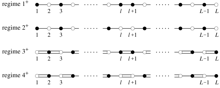
Figure 2: Groundstate configurations for the four different regimes.

5.2 Local height probabilities

The local height probability $P^{bc}(a)$ is the probability that a given site of the lattice has height $a$ given that the model is in the phase indexed by $b$ and $c$. In the ferromagnetic phases $c=b$ and in the antiferromagnetic phases $c=b\pm 1$.

The technique of corner transfer matrices (CTMs) which is used to calculate $P^{bc}(a)$ is well-known and the details of the method are given elsewhere (see, e.g., [14, 1]). Because the weights (3.25) satisfy the Yang-Baxter equation and possess the crossing symmetry (3.49), the local height probability in regimes $1^{+}$ and $2^{+}$ can be written as

$$P^{bc}(a)=\lim_{m\rightarrow\infty}\frac{q^{-a^{2}\lambda/\pi}S(a)X_{m}^{a\,b\,c}(q)}{\sum_{a=1}^{L}q^{-a^{2}\lambda/\pi}S(a)X_{m}^{a\,b\,c}(q)}\,.$$ (5.2)

Here the variable $q$ is related to $p=\exp(-\epsilon)$ by

$$q=\mbox{e}^{-12\pi\lambda/\epsilon}.$$ (5.3)

The one-dimensional configuration sums $X_{m}^{a\,b\,c}(q)$ are given by

$$X_{m}^{\sigma_{1}\,\sigma_{m+1}\,\sigma_{m+2}}(q)=\sum_{\sigma_{2},\ldots,\sigma_{m}}q^{\sum_{j=1}^{m}jH(\sigma_{j},\sigma_{j+1},\sigma_{j+2})}.$$ (5.4)

The weight function $H$ is determined from the Boltzmann weights in the ordered limit ($p\rightarrow 1,u/\epsilon$ fixed). Their behaviour is

$$W\left(\begin{array}[]{cc}d&c\\ a&b\end{array}\right)\sim\frac{g_{a}g_{c}}{g_{b}g_{d}}\;\mbox{e}^{-2\pi uH(d,a,b)/\epsilon}\>\delta_{a,c}$$ (5.5)

where

$$g_{a}=\mbox{e}^{-2\lambda ua^{2}/\epsilon}.$$ (5.6)

The values of the function $H(d,a,b)$ for regimes $1^{+}$ and $2^{+}$ are listed in appendix A.

From (5.4) it follows directly that the one-dimensional configuration sums satisfy the following recurrence relation:

$$X_{m}^{a\,b\,c}(q)=q^{mH(b-1,b,c)}X_{m-1}^{a\,b-1\,b}(q)+q^{mH(b,b,c)}X_{m-1}^{a\,b\,b}(q)+q^{mH(b+1,b,c)}X_{m-1}^{a\,b+1\,b}(q).$$ (5.7)

The task is to solve this relation, with initial condition

$$X_{1}^{a\,b\,c}(q)=q^{H(a,b,c)}$$ (5.8)

or, equivalently,

$$X_{0}^{a\,b\,c}(q)=\delta_{a,b}$$ (5.9)

and with the conditions

$$X_{m}^{a\,0\,1}(q)=X_{m}^{a\,L+1\,L}(q)=0$$ (5.10)

which confine the heights in the recursion relation (5.7) to the set $\{1,\ldots,L\}$.

In regimes $3^{+}$ and $4^{+}$, where the spectral parameter $u$ is negative, the local height probability is given by

$$P^{bc}(a)=\lim_{m\rightarrow\infty}\frac{q^{a^{2}\lambda/\pi}S(a)X_{m}^{a\,b\,c}(q)}{\sum_{a=1}^{L}q^{a^{2}\lambda/\pi}S(a)X_{m}^{a\,b\,c}(q)}$$ (5.11)

where $q$ is now

$$q=\mbox{e}^{-4\pi(\pi-3\lambda)/\epsilon}.$$ (5.12)

As for the regimes 1⁺ and 2⁺, the one-dimensional configuration sums are expressed in $H$ by (5.4). To determine $H$, we now need to know the powers of $\mbox{e}^{+2\pi u/\epsilon}$ in the ordered limit of the weights. Relative to regimes 1⁺ and 2⁺, after the appropriate gauge factors $g$ are separated, and contributions which cancel in the ratio in equation (5.11) are discarded, $H$ is effectively replaced $-H$. We thus need only take $q\rightarrow 1/q$ in the regime $1^{+}$ ($2^{+}$) solution of (5.7) to obtain the form of the solution in regime $4^{+}$ ($3^{+}$). Of course, $q$ must still be given its proper meaning from (5.12).

5.3 Solution of the recurrence relation

In this section we derive the solution of the recursion relation (5.7) for each of the four regimes. In fact, as remarked above, the solution for regimes $3^{+}$ and $4^{+}$ is deduced from the solution for regimes $1^{+}$ and $2^{+}$.

Gaussian multinomials

Before we present the solution we need some preliminaries on the Gaussian multinomials $\left[{\textstyle{m\atop k,l}}\right]$, defined by [19]

$$\left[m\atop k,l\right]=\left[m\atop k,l\right]_{q}=\frac{(q)_{m}}{(q)_{k}(q)_{l}(q)_{m-k-l}}$$ (5.13)

where

$$(q)_{m}=\prod_{k=1}^{m}(1-q^{k}).$$ (5.14)

In the limit $q\to 1$ the Gaussian multinomials reduce to ordinary multinomials

$$\lim_{q\rightarrow 1}\left[m\atop k,l\right]=\frac{m!}{k!\>l!\>(m\!-\!k\!-\!l)!}={m\choose k,l}.$$ (5.15)

The following identities, which prove useful in solving the recurrence relation, may be derived by straightforward manipulation of the definition

$$\left[m\atop k,l\right] = \left[m-1\atop k,l\right]+q^{m-k}\left[m-1\atop k-1,l\right]+q^{m-k-l}\left[m-1\atop k,l-1\right]$$ (5.16)

$$= \left[m-1\atop k-1,l\right]+q^{m-l}\left[m-1\atop k,l-1\right]+q^{k}\left[m-1\atop k,l\right]$$ (5.17)

$$= \left[m-1\atop k-1,l\right]+q^{k+l}\left[m-1\atop k,l\right]+q^{k}\left[m-1\atop k,l-1\right].$$ (5.18)

Regime 1⁺

As a first step towards the solution of equation (5.7) we consider the special limit $q=1$.
In this limit, setting $X_{m}^{a\,b\,c}(1)=X_{m}^{a\,b\,c}$, the recurrence relation reduces to the following combinatorial problem

$$X_{m}^{a\,b\,c}=X_{m-1}^{a\,b-1\,b}+X_{m-1}^{a\,b\,b}+X_{m-1}^{a\,b+1\,b}.$$ (5.19)

The fundamental solution of this equation is

$$X_{m}^{a\,b\,c}=\sum_{k=0}^{\infty}{m\choose k,k\!+\!b}.$$ (5.20)

In order to satisfy the initial and confining conditions (5.9) and (5.10) we must take linear combinations of this solution in the following way:

$$X_{m}^{a\,b\,c}=\sum_{j,k=-\infty}^{\infty}\left\{{m\choose k,k\!+\!2(L\!+\!1)j\!+\!a\!-\!b}-{m\choose k,k\!+\!2(L\!+\!1)j\!+\!a\!+\!b}\right\}.$$ (5.21)

Another piece of information can be gained by considering the $m\rightarrow\infty$ limit. It was noted in [20] that, in this limit, the one-dimensional configuration sums for the ABF models in regimes III and IV become precisely the characters of the related Virasoro algebra (1.4).

Expecting similar $m\rightarrow\infty$ behaviour for our configuration sums, we generated large polynomials on the computer and multiplied these by $Q(q)$. The resulting polynomials, being very sparse, were then easily identified as Virasoro characters, with $r=a$ and $s=b$ for $b\leq l$ and $s=b+1$ for $b>l$, or as linear combinations of two characters.

Guided by these two limiting cases, replacing $h$ in (1.4) by $L+2$ according to (1.6), we make the following Ansatz for the configuration sums, with $b\leq l$, which yield a single character:

$$X_{m}^{a\,b\,c}=q^{\gamma\,m}\!\sum_{j,k=-\infty}^{\infty}\left\{q^{(L+2)(L+1)j^{2}+[(L+2)a-(L+1)b]j+\alpha(j,k)}\left[m\atop k,k\!+\!2(L\!+\!1)j\!+\!a\!-\!b\right]\right.$$

$$\hphantom{X_{m}^{a\,b\,c}=q^{\gamma\,m}\!\sum_{j,k=-\infty}^{\infty}}\hskip 0.0pt\hskip 0.0pt\left.-q^{(L+2)(L+1)j^{2}+[(L+2)a+(L+1)b]j+ab+\beta(j,k)}\left[m\atop k,k\!+\!2(L\!+\!1)j\!+\!a\!+\!b\right]\right\}.$$ (5.22)

For $b>l$ we make a similar Ansatz. The unknown functions $\alpha$ and $\beta$ are assumed to be quadratic in their arguments $j$ and $k$. They depend implicitly on $a$, $b$ and $c$, as does the parameter $\gamma$. For the configuration sums that, in the $m\rightarrow\infty$ limit, yield linear combinations of characters, we make the appropriate linear combinations of the above Ansatz.

Fitting the Ansatz for small values of $m$ with the correct polynomial, the coefficients in the functions $\alpha(j,k)$ $\beta(j,k)$ and $\gamma$ can be determined. Before we present the solution, we define the following auxiliary function:

$$F_{m}^{s}(b)=q^{(a-s)a/2}\sum_{j,k=-\infty}^{\infty}$$

$$\qquad\quad\left\{q^{(L+2)(L+1)j^{2}+[(L+2)a-(L+1)s]j+k[k+2(L+1)j+a-b]}\left[m\atop k,k\!+\!2(L\!+\!1)j\!+\!a\!-\!b\right]\right.$$ (5.23)

$$\hskip 0.0pt\left.\qquad\quad-q^{(L+2)(L+1)j^{2}+[(L+2)a+(L+1)s]j+as+k[k+2(L+1)j+a+b]}\left[m\atop k,k\!+\!2(L\!+\!1)j\!+\!a\!+\!b\right]\right\}$$

where we have suppressed the $a$ dependence. This function has the following elementary properties

$$F_{m}^{s}(b)=-F_{m}^{-s}(-b)$$

$$F_{m}^{L+2+s}(L\!+\!1\!+\!b)=-q^{-(L+1)s}F_{m}^{L+2-s}(L\!+\!1\!-\!b)\vphantom{\sum_{a}^{a}}$$ (5.24)

$$F_{m}^{1}(0)=(1\!-\!q^{m})F_{m-1}^{1}(1).$$

It is also convenient to define the four sets

$$s_{1} = \{1,3,\ldots,l\}$$

$$s_{2} = \{l+1,l+3,\ldots,L-1\}$$

$$s_{3} = \{2,4,\ldots,l-1\}$$ (5.25)

$$s_{4} = \{l+2,l+4,\ldots,L\}$$

where $l$ is given by (5.1). With these definitions the solution of the recurrence relation reads

$$\begin{array}[]{rll}X_{m}^{a\,b\,b-1}=q^{mH(b,b,b-1)}\times&\left\{\begin{array}[]{l}F_{m}^{b}(b)\\ q^{\frac{1}{2}b}F_{m}^{b+1}(b)\\ q^{\frac{1}{2}b}F_{m}^{b+1}(b)\\ F_{m}^{b}(b)+(1\!-\!q^{m})q^{b}F_{m\!-\!1}^{b+2}(b\!+\!1)\end{array}\right.&\begin{array}[]{l}b\in s_{1}\setminus\{1\}\\ b\in s_{2}\cup\{L\!+\!1\}\\ b\in s_{3}\\ b\in s_{4}\end{array}\\ &&\\ X_{m}^{a\,b\,b}=q^{mH(b,b,b)}\times&\left\{\begin{array}[]{l}F_{m}^{b}(b)\\ q^{\frac{1}{2}b}F_{m}^{b+1}(b)\\ q^{\frac{1}{2}b}F_{m}^{b+1}(b)+(1\!-\!q^{m})q^{-\frac{1}{2}b}F_{m\!-\!1}^{b-1}(b\!-\!1)\\ F_{m}^{b}(b)+(1\!-\!q^{m})q^{b}F_{m\!-\!1}^{b+2}(b\!+\!1)\end{array}\right.&\begin{array}[]{l}b\in s_{1}\\ b\in s_{2}\\ b\in s_{3}\\ b\in s_{4}\end{array}\\ &&\\ X_{m}^{a\,b\,b+1}=q^{mH(b,b,b+1)}\times&\left\{\begin{array}[]{l}F_{m}^{b}(b)\\ q^{\frac{1}{2}b}F_{m}^{b+1}(b)\\ q^{\frac{1}{2}b}F_{m}^{b+1}(b)+(1\!-\!q^{m})q^{-\frac{1}{2}b}F_{m\!-\!1}^{b-1}(b\!-\!1)\\ F_{m}^{b}(b)\end{array}\right.&\begin{array}[]{l}b\in s_{1}\\ b\in s_{2}\\ b\in s_{3}\cup\{0\}\\ b\in s_{4}\setminus\{L\}.\end{array}\end{array}$$ (5.26)

We note that in this solution we have included the terms $X_{m}^{a\,0\,1}$ and $X_{m}^{a\,L+1\,L}$ which, according to the confining condition (5.10), should be identically zero. Using the simple relations (5.24) it follows directly that this is indeed the case. The advantage of including these terms in the above way is that it enables us to prove the solution without treating the boundary separately. From the definition (5.23) it also follows immediately that the initial condition (5.9) is satisfied.

Proving that (5.26) is indeed the solution of the recurrence relation is now straightforward but rather tedious. Inserting (5.26) into the recursion relation, using the explicit form of the function $H$ as listed in equation (LABEL:eq:A.HfuncR1), we find that only the following four relations need hold:

$$\begin{array}[]{ll}F_{m}^{b}(b)-F_{m-1}^{b}(b)\vphantom{\displaystyle\sum_{a}}&\\ \qquad=q^{m-1}\left[F_{m-1}^{b}(b\!-\!1)+q^{b+1}F_{m-1}^{b+2}(b\!+\!1)+q^{-b+1}(1\!-\!q^{m-1})F_{m-2}^{b-2}(b\!-\!2)\right]&b\in s_{1}\\ F_{m}^{b+1}(b)-F_{m-1}^{b+1}(b)\vphantom{\displaystyle\sum_{a}^{a}}&\\ \qquad=q^{m-1}\left[F_{m-1}^{b+1}(b\!+\!1)+q^{-b+1}F_{m-1}^{b-1}(b\!-\!1)+q^{b+1}(1\!-\!q^{m-1})F_{m-2}^{b+3}(b\!+\!2)\right]&b\in s_{2}\\ F_{m}^{b+1}(b)-F_{m-1}^{b+1}(b\!+\!1)\vphantom{\displaystyle\sum_{a}^{a}}&\\ \qquad=q^{m-1}\left[F_{m-1}^{b+1}(b)+q^{-b+1}F_{m-1}^{b-1}(b\!-\!1)+q^{-b}(1\!-\!q^{m-1})F_{m-2}^{b-1}(b\!-\!1)\right]&b\in s_{3}\\ F_{m}^{b}(b)-F_{m-1}^{b}(b\!-\!1)\vphantom{\displaystyle\sum_{a}^{a}}&\\ \qquad=q^{m-1}\left[F_{m-1}^{b}(b)+q^{b+1}F_{m-1}^{b+2}(b\!+\!1)+q^{b}(1\!-\!q^{m-1})F_{m-2}^{b+2}(b\!+\!1)\right]&b\in s_{4}.\end{array}$$ (5.27)

The restrictions on $b$ make these special cases of more general expressions, which we will show to be true for all values of $b$. If we widen their applicability in this way, the relations can in fact be combined to give simpler ones. In turn, these relations can be further simplified by requiring that they hold term-by-term in $j$. The resulting pair of relations are much stronger requirements than the original set, but still they hold. Defining the function

$$f_{m}^{s}(b)=\sum_{k=0}^{\infty}\left\{q^{-\frac{1}{2}\gamma s+k(k+\gamma-b)}\left[m\atop k,k+\gamma-b\right]-q^{\frac{1}{2}\gamma s+k(k+\gamma+b)}\left[m\atop k,k+\gamma+b\right]\right\}$$ (5.28)

where we have set $2(L+1)j+a=\gamma$, these two relations are

$$f_{m}^{b}(b)-f_{m}^{b}(b\!-\!1)=q^{m}\left[q^{b}f_{m-1}^{b+2}(b\!+\!1)-q^{-b+1}f_{m-1}^{b-2}(b\!-\!2)\right]$$ (5.29)

$$f_{m}^{b}(b)-f_{m-1}^{b}(b)=q^{m-1}\left[f_{m-1}^{b}(b\!-\!1)+q^{b+1}f_{m-1}^{b+2}(b\!+\!1)+q^{-b+1}(1\!-\!q^{m-1})f_{m-2}^{b-2}(b\!-\!2)\right]\!.$$ (5.30)

The function $f_{m}^{s}$ consists of two polynomials. One, the first term within the curly braces, has only positive coefficients and the other, the second term, has only negative coefficients. If we demand that the equations (5.29) and (5.30) be satisfied for the ‘positive’ and ‘negative’ polynomials independently, and we set $\gamma\mp b=n$, respectively, this yields

$$\sum_{k=0}^{\infty}q^{k(k+n)}\left[m\atop k,k+n\right]-\sum_{k=0}^{\infty}q^{k(k+n+1)}\left[m\atop k,k+n+1\right]$$ (5.31)

$$=q^{m-n}\sum_{k=0}^{\infty}q^{k(k+n-1)}\left[m-1\atop k,k+n-1\right]-q^{m+n+1}\sum_{k=0}^{\infty}q^{k(k+n+2)}\left[m-1\atop k,k+n+2\right]$$

for equation (5.29), and

$$\sum_{k=0}^{\infty}q^{k(k+n)}\left[m\atop k,k+n\right]-\sum_{k=0}^{\infty}q^{k(k+n)}\left[m-1\atop k,k+n\right]$$

$$=q^{m-1}\sum_{k=0}^{\infty}q^{k(k+n+1)}\left[m-1\atop k,k+n+1\right]-q^{m-n}\sum_{k=0}^{\infty}q^{k(k+n-1)}\left[m-1\atop k,k+n-1\right]$$

$$+q^{m+n}(1-q^{m-1})\sum_{k=0}^{\infty}q^{k(k+n+2)}\left[m-2\atop k,k+n+2\right]$$

for equation (5.30). The proof of these final two equations is now elementary. Equation (5.31) follows immediately from (5.16) and (5.17) if we set $l=k+n$ and $l=k+n+1$, respectively. Equation (5.3) follows from (5.16) with $l=k+n$.

Regime 2⁺

Finding and proving the solution of the recurrence relation for regime $2^{+}$ proceeds along similar lines as in regime $1^{+}$. To remove any confusion we will denote the one-dimensional configuration sums in regime $2^{+}$ by $Y_{m}^{a\,b\,c}$. First of all, the $q=1$ limit (5.21) is still valid. Generating large polynomials reveals that in this case the configuration sums yield Virasoro characters with $s=a$ and $r=b$ for $b\leq l-1$, and $r=b-1$ for $b\geq l+2$, or linear combinations of two characters.

We replace $h$ in (1.4) by $L+1$ according to (1.6) and define the auxiliary function

$$G_{m}^{r}(b)=q^{(a-r)a/2}\sum_{j,k=-\infty}^{\infty}$$

$$\quad\qquad\left\{q^{(L+1)Lj^{2}-[(L+1)r-La]j+k[k+2(L+1)j+a-b]}\left[m\atop k,k\!+\!2(L\!+\!1)j\!+\!a\!-\!b\right]\right.$$ (5.33)

$$\quad\qquad\left.\hskip 0.0pt-q^{(L+1)Lj^{2}+[(L+1)r+La]j+ar+k[k+2(L+1)j+a+b]}\left[m\atop k,k\!+\!2(L\!+\!1)j\!+\!a\!+\!b\right]\right\}$$

which satisfies the following simple relations

$$G_{m}^{r}(b)=-G_{m}^{-r}(-b)$$

$$G_{m}^{L+r}(L\!+\!1\!+\!b)=-q^{-(L+1)r}G_{m}^{L-r}(L+1-b)\vphantom{\sum_{a}^{a}}$$ (5.34)

$$G_{m}^{1}(0)=(1\!-\!q^{m})G_{m-1}^{1}(1).$$

Again we define four sets

$$t_{1} = \{1,3,\ldots,l-1\}$$

$$t_{2} = \{l+2,l+3,\ldots,L-1\}$$

$$t_{3} = \{2,4,\ldots,l\}$$ (5.35)

$$t_{4} = \{l+1,l+3,\ldots,L\}.$$

The solution of the recurrence relation then reads

$$\begin{array}[]{rll}Y_{m}^{a\,b\,b-1}=q^{mH(b,b,b-1)}\times&\left\{\!\!\begin{array}[]{l}G_{m}^{b}(b)\\ q^{-\frac{1}{2}b}G_{m}^{b-1}(b)\\ q^{-\frac{1}{2}b}G_{m}^{b-1}(b)+(1\!-\!q^{m})q^{\frac{1}{2}b}G_{m-1}^{b+1}(b\!+\!1)\\ \hphantom{q^{-\frac{1}{2}b}G_{m}^{b-1}(b)}-(1\!-\!q^{m})q^{-1}G_{m-1}^{1}(1)\delta_{b,2}\\ G_{m}^{b}(b)\end{array}\right.&\begin{array}[]{l}b\in t_{1}\setminus\{1\}\\ b\in t_{2}\cup\{L\!+\!1\}\\ \\ b\in t_{3}\\ b\in t_{4}\end{array}\\ &&\\ Y_{m}^{a\,b\,b}=q^{mH(b,b,b)}\times&\left\{\!\!\begin{array}[]{l}G_{m}^{b}(b)\\ q^{-\frac{1}{2}b}G_{m}^{b-1}(b)\\ q^{-\frac{1}{2}b}G_{m}^{b-1}(b)+(1\!-\!q^{m})q^{\frac{1}{2}b}G_{m-1}^{b+1}(b\!+\!1)\\ G_{m}^{b}(b)+(1\!-\!q^{m})q^{-b}G_{m-1}^{b-2}(b\!-\!1)\end{array}\right.&\begin{array}[]{l}b\in t_{1}\\ b\in t_{2}\\ b\in t_{3}\\ b\in t_{4}\end{array}\\ &&\\ Y_{m}^{a\,b\,b+1}=q^{mH(b,b,b+1)}\times&\left\{\!\!\begin{array}[]{l}G_{m}^{b}(b)\\ q^{-\frac{1}{2}b}G_{m}^{b-1}(b)\\ q^{-\frac{1}{2}b}G_{m}^{b-1}(b)\\ G_{m}^{b}(b)+(1\!-\!q^{m})q^{-b}G_{m-1}^{b-2}(b\!-\!1)\end{array}\right.&\begin{array}[]{l}b\in t_{1}\\ b\in t_{2}\\ b\in t_{3}\\ b\in t_{4}\setminus\{L\}.\end{array}\end{array}$$ (5.36)

As in regime $1^{+}$ we have extended the solution to include the term $Y_{m}^{a\,L+1\,L}$, which, using (5.34), indeed yields zero. However, in contrast to regime $1^{+}$, we can no longer extend the above solution to the term $Y_{m}^{a\,0\,1}$ which according to (5.36) would not be zero. Therefore, in proving the recurrence relation we have to treat cases that involve this boundary term separately. This ‘irregularity’ is however compensated by the exceptional terms $Y_{m}^{a\,2\,1}$ of (5.36) and $H(1,2,1)$ of (LABEL:eq:A.HfuncR2). As a result, inserting the above solution into the recurrence relation, using (5.34), we again obtain only four relations that should hold:

$$\begin{array}[]{ll}G_{m}^{b}(b)-G_{m-1}^{b}(b)\vphantom{\displaystyle\sum_{a}}&\\ \qquad=q^{m-1}\!\left[G_{m-1}^{b}(b\!+\!1)+q^{-b+1}G_{m-1}^{b-2}(b\!-\!1)+q^{b+1}(1\!-\!q^{m-1})G_{m-2}^{b+2}(b\!+\!2)\right]&b\in t_{1}\\ G_{m}^{b-1}(b)-G_{m-1}^{b-1}(b)\vphantom{\displaystyle\sum_{a}^{a}}&\\ \qquad=q^{m-1}\!\left[G_{m-1}^{b-1}(b\!-\!1)+q^{b+1}G_{m-1}^{b+1}(b\!+\!1)+q^{-b+1}(1\!-\!q^{m-1})G_{m-2}^{b-3}(b\!-\!2)\right]&b\in t_{2}\\ G_{m}^{b-1}(b)-G_{m-1}^{b-1}(b\!-\!1)\vphantom{\displaystyle\sum_{a}^{a}}&\\ \qquad=q^{m-1}\!\left[G_{m-1}^{b-1}(b)+q^{b+1}G_{m-1}^{b+1}(b\!+\!1)+q^{b}(1\!-\!q^{m-1})G_{m-2}^{b+1}(b\!+\!1)\right]&b\in t_{3}\\ G_{m}^{b}(b)-G_{m-1}^{b}(b\!+\!1)\vphantom{\displaystyle\sum_{a}^{a}}&\\ \qquad=q^{m-1}\!\left[G_{m-1}^{b}(b)+q^{-b+1}G_{m-1}^{b-2}(b\!-\!1)+q^{-b}(1\!-\!q^{m-1})G_{m-2}^{b-2}(b\!-\!1)\right]&b\in t_{4}.\end{array}$$ (5.37)

Again these equations hold for all values of $b$ and we drop the restrictions on $b$. Doing so, the four equations can be combined to give simpler equations. As before, these are true term-by-term in $j$. Setting $2(L+1)j+a=\gamma$, we find

$$f_{m}^{b}(b)-f_{m}^{b}(b\!+\!1)=q^{m}\left[q^{-b}f_{m-1}^{b-2}(b\!-\!1)-q^{b+1}f_{m-1}^{b+2}(b\!+\!2)\right]$$

$$f_{m}^{b}(b)-f_{m-1}^{b}(b)=q^{m-1}\left[f_{m-1}^{b}(b\!+\!1)+q^{-b+1}f_{m-1}^{b-2}(b\!-\!1)+q^{b+1}(1\!-\!q^{m-1})f_{m-2}^{b+2}(b\!+\!2)\right]$$ (5.38)

with $f_{m}^{s}$ defined in (5.28). Finally, making the same splitting into ‘positive’ and ‘negative’ polynomials as before, now setting $\gamma\mp b=-n$, yields precisely the equations (5.31) and (5.3).

Regimes 3⁺ and 4⁺

As explained previously, the form of the solution of the recurrence relation for regimes $3^{+}$ and $4^{+}$ can simply be obtained by replacing $q$ with $1/q$ in (5.36) and (5.26), respectively. It should again be stressed that the precise meaning of the variable $q$ in the various regimes is not related, and is given by equation (5.3) in regimes $1^{+}$ and $2^{+}$, and by (5.12)in regimes 3⁺ and 4⁺.

5.4 Thermodynamic limit

In this section, using the solutions for the one-dimensional configuration sums $X_{m}^{a\,b\,c}$ and $Y_{m}^{a\,b\,c}$, we obtain expressions for the local height probabilities $P^{bc}(a)$.

Regime 1⁺

As described in section 5.1, in regime 1⁺ we have only ferromagnetic groundstate configurations. Hence we need to calculate

$$P^{bb}(a)=\lim_{m\rightarrow\infty}\frac{q^{-a^{2}\lambda/\pi}S(a)X_{m}^{a\,b\,b}(q)}{\sum_{a=1}^{L}q^{-a^{2}\lambda/\pi}S(a)X_{m}^{a\,b\,b}(q)}\qquad b=1,3,\ldots,l,l+1,l+3,\ldots,L-1.$$ (5.39)

From the solution (5.26) for the one-dimensional configuration sums, we find that we have to consider the $m\to\infty$ limit of the auxiliary function $F_{m}^{s}$ defined in (5.23). To do so, we need the result

$$\lim_{m\to\infty}\sum_{k=-\infty}^{\infty}q^{k(k+a)}\left[m\atop k,k+a\right]_{q}=\frac{1}{Q(q)}$$ (5.40)

which holds for arbitrary fixed $a$. To establish this we take the limit inside the sum and use the elementary result

$$\lim_{m\to\infty}\left[m\atop k,k+a\right]_{q}=\lim_{m\to\infty}\;\frac{(q)_{m}}{(q)_{k}\,(q)_{k+a}\,(q)_{m-2k-a}}=\frac{1}{(q)_{k}\,(q)_{k+a}}$$ (5.41)

to obtain

$$\lim_{m\to\infty}\sum_{k=-\infty}^{\infty}q^{k(k+a)}\left[m\atop k,k+a\right]_{q}=\sum_{k=0}^{\infty}\frac{q^{k(k+a)}}{(q)_{k}\,(q)_{k+a}}=\frac{1}{Q(q)}\,.$$ (5.42)

Here the last equality follows from the $q$-analogue of Kummer’s theorem [19]

$$\sum_{k=0}^{\infty}\frac{q^{k(k-1)}z^{k}}{(1-q)\ldots(1-q^{k})(1-z)(1-zq)\ldots(1-zq^{k-1})}=\prod_{k=0}^{\infty}\frac{1}{1-zq^{k}}$$ (5.43)

by setting $z=q^{a+1}$. From the above considerations we conclude that, in the $m\to\infty$ limit, the auxiliary function $F_{m}^{s}$ yields the Virasoro characters defined in equation (1.4)

$$\lim_{m\to\infty}F_{m}^{s}(b)=\frac{q^{\frac{1}{2}(a-s)a}}{Q(q)}\sum_{j=-\infty}^{\infty}\left\{q^{(L+2)(L+1)j^{2}+[(L+2)a-(L+1)s]j}\!-\!q^{(L+2)(L+1)j^{2}+[(L+2)a+(L+1)s]j+as}\right\}$$

$$\hphantom{\lim_{m\to\infty}F_{m}^{s}(b)}\vphantom{\sum^{a}_{a}}=q^{\frac{1}{2}(a-s)a-\Delta_{a,s}^{(L+2)}+c/24}\>\chi_{a,s}^{(L+2)}(q)$$ (5.44)

$$\hphantom{\lim_{m\to\infty}F_{m}^{s}(b)}\sim q^{a^{2}\lambda/\pi}\>\chi_{a,s}^{(L+2)}(q).$$

In the last step we have used $\lambda=\pi L/(4(L+1))$, and have omitted terms independent of $a$.

Substituting the appropriate elements of the solution (5.26), the $X_{m}^{a\,b\,b}$, into the expression for local height probabilities, and using the limiting behaviour of $F_{m}^{s}$, we find

$$P^{bb}(a)=\frac{S(a)\chi_{a,s}^{(L+2)}(q)}{\sum_{a=1}^{L}S(a)\chi_{a,s}^{(L+2)}(q)}$$ (5.45)

where

$$s=\left\{\begin{array}[]{ll}b&\qquad b=1,3,\ldots,l\\ b+1&\qquad b=l+1,l+3,\ldots,L-1.\end{array}\right.$$ (5.46)

We note that $s$ takes the values $1,3,\ldots,L$.

By performing the conjugate modulus transformation (C.11) we rewrite the Virasoro characters as

$$\chi_{r,s}^{(h)}(q)=\frac{q^{-c/24-1/4h(h-1)}}{Q(q)}\left(\frac{\epsilon^{\prime}}{\pi}\right)^{1/2}\left[\vartheta_{3}\!\left({\textstyle{\pi\over 2}}\left({\textstyle{r\over h-1}}\!-\!{\textstyle{s\over h}}\right),t\right)-\vartheta_{3}\!\left({\textstyle{\pi\over 2}}\left({\textstyle{r\over h-1}}\!+\!{\textstyle{s\over h}}\right),t\right)\right]$$ (5.47)

where

$$q^{h(h-1)}=\mbox{e}^{-\pi^{2}/\epsilon^{\prime}}\qquad\mbox{and}\qquad t=\mbox{e}^{-\epsilon^{\prime}}.$$ (5.48)

As a result the local height probabilities can be written in the form

$$P^{bb}(a)=\frac{S(a)}{N_{1}(s)}\left[\vartheta_{3}\!\left({\textstyle{\pi\over 2}}\left({\textstyle{a\over L+1}}\!-\!{\textstyle{s\over L+2}}\right),t\right)-\vartheta_{3}\!\left({\textstyle{\pi\over 2}}\left({\textstyle{a\over L+1}}\!+\!{\textstyle{s\over L+2}}\right),t\right)\right]$$ (5.49)

where the normalisation factor in the denominator is given by

$$N_{1}(s) = \sum_{a=1}^{L}S(a)\left[\vartheta_{3}\left({\textstyle{\pi\over 2}}\left({\textstyle{a\over L+1}}\!-\!{\textstyle{s\over L+2}}\right),t\right)-\vartheta_{3}\left({\textstyle{\pi\over 2}}\left({\textstyle{a\over L+1}}\!+\!{\textstyle{s\over L+2}}\right),t\right)\right]$$ (5.50)

$$= \sum_{a=0}^{2L+1}S(a)\,\vartheta_{3}\left({\textstyle{\pi\over 2}}\left({\textstyle{a\over L+1}}\!-\!{\textstyle{s\over L+2}}\right),t\right).$$

We recall that the nome $q$ is defined in terms of the nome $p$ as $q=\exp(-12\pi\lambda/\epsilon)$. This yields the following relation between the nomes $p$ and $t$:

$$p=t^{3L(L+2)}.$$ (5.51)

From the definition of the crossing factor

$$S(a)=(-1)^{a}\frac{\vartheta_{1}\left(4a\lambda,p\right)}{\vartheta_{4}\left(2a\lambda,p\right)}$$ (5.52)

and the simple identity

$$\frac{\vartheta_{1}(2u,p)}{\vartheta_{4}(u,p)}=\frac{\vartheta_{1}(2u,p^{2})\vartheta_{3}(u,p)}{p^{1/4}Q(p^{2})Q(p^{4})}$$ (5.53)

we find an alternative form for $S$:

$$S(a)=\vartheta_{1}\!\left({\textstyle{a\pi\over L+1}},t^{6L(L+2)}\right)\vartheta_{3}\!\left({\textstyle{a\pi L\over 2(L+1)}},t^{3L(L+2)}\right)$$ (5.54)

where we have again neglected $a$-independent factors. Substituting this back into the definition of the normalisation factor, we find that the summation in $N_{1}(s)$ can actually be performed to give

$$\frac{S(a)}{N_{1}(s)}=\frac{t^{-L(2L+3)/2}\>\vartheta_{1}\!\left({\textstyle{a\pi\over L+1}},t^{6L(L+2)}\right)\vartheta_{3}\!\left({\textstyle{a\pi L\over 2(L+1)}},t^{3L(L+2)}\right)\vartheta_{2}\!\left({\textstyle{s\pi\over L+2}},t^{6L(L+1)}\right)}{2(L+1)Q\left(t^{12L(L+1)}\right)Q\left(t^{12L(L+2)}\right)\vartheta_{1}\!\left({\textstyle{\pi\over 6}},t^{2(L+1)(L+2)}\right)\vartheta_{1}\!\left({\textstyle{2s\pi\over L+2}},t^{6L(L+1)}\right)}\,.$$ (5.55)

The proof of this denominator identity, being rather technical and lengthy, is given in appendix B.1.

Regime 2⁺

The working for regime 2⁺ is very similar to that of regime 1⁺. Again we have only ferromagnetic groundstates, and we are interested in calculating

$$P^{bb}(a)=\lim_{m\rightarrow\infty}\frac{q^{-a^{2}\lambda/\pi}S(a)Y_{m}^{a\,b\,b}(q)}{\sum_{a=1}^{L}q^{-a^{2}\lambda/\pi}S(a)Y_{m}^{a\,b\,b}(q)}\;\quad b=1,3,\ldots,l-1,l+2,l+4,\ldots,L-1.$$ (5.56)

From the solution (5.36) for the one-dimensional configuration sums we see that we have to take the limit $m\to\infty$ of the auxiliary function $G_{m}^{r}$ defined in (5.33). Using the result (5.40) yields

$$\lim_{m\to\infty}G_{m}^{r}(b)=\frac{q^{\frac{1}{2}(a-r)a}}{Q(q)}\sum_{j=-\infty}^{\infty}\left\{q^{(L+1)Lj^{2}-[(L+1)r-La]j}\!-\!q^{(L+1)Lj^{2}+[(L+1)r+La]j+ar}\right\}$$

$$\hphantom{\lim_{m\to\infty}G_{m}^{s}(b)}\vphantom{\sum^{a}_{a}}=q^{\frac{1}{2}(a-r)a-\Delta_{r,a}^{(L+1)}+c/24}\>\chi_{r,a}^{(L+1)}(q)$$ (5.57)

$$\hphantom{\lim_{m\to\infty}G_{m}^{s}(b)}\sim q^{a^{2}\lambda/\pi}\>\chi_{r,a}^{(L+1)}(q)$$

where we have used that $\lambda=\pi(L+2)/(4(L+1))$.

Substituting the elements $Y_{m}^{a\,b\,b}$ of the solution (5.36), and using the limiting behaviour of $G_{m}^{r}$, we find that the local height probabilities are given by

$$P^{bb}(a)=\frac{S(a)\chi_{r,a}^{(L+1)}(q)}{\sum_{a=1}^{L}S(a)\chi_{r,a}^{(L+1)}(q)}$$ (5.58)

where

$$r=\left\{\begin{array}[]{ll}b&\qquad b=1,3,\ldots,l-1\\ b-1&\qquad b=l+2,l+4,\ldots,L-1.\end{array}\right.$$ (5.59)

We note that $r$ takes the values $1,3,\ldots,L-2$.

If we use the conjugate modulus form of the Virasoro characters, we can rewrite this as

$$P^{bb}(a)=\frac{S(a)}{N_{2}(r)}\left[\vartheta_{3}\!\left({\textstyle{\pi\over 2}}\left({\textstyle{r\over L}}\!-\!{\textstyle{a\over L+1}}\right),t\right)-\vartheta_{3}\!\left({\textstyle{\pi\over 2}}\left({\textstyle{r\over L}}\!+\!{\textstyle{a\over L+1}}\right),t\right)\right]$$ (5.60)

where the normalisation factor in the denominator is

$$N_{2}(r)=\sum_{a=0}^{2L+1}S(a)\,\vartheta_{3}\left({\textstyle{\pi\over 2}}\left({\textstyle{r\over L}}\!-\!{\textstyle{a\over L+1}}\right),t\right).$$ (5.61)

From the relation between the nomes $p$ and $q$ we find that $p$ and $t$ are again related as in equation (5.51). Inserting the form (5.54) for the crossing factor $S$ into the expression for the normalisation factor $N_{2}$, we can carry out the summation over $a$. The result, proved in appendix B.2, is

$$\frac{S(a)}{N_{2}(r)}=\frac{t^{-(L+2)(2L+1)/2}\>\vartheta_{1}\!\left({\textstyle{a\pi\over L+1}},t^{6L(L+2)}\right)\vartheta_{3}\!\left({\textstyle{a\pi L\over 2(L+1)}},t^{3L(L+2)}\right)\vartheta_{2}\!\left({\textstyle{r\pi\over L}},t^{6(L+1)(L+2)}\right)}{2(L+1)Q\left(t^{12L(L+2)}\right)Q\left(t^{12(L+1)(L+2)}\right)\vartheta_{1}\!\left({\textstyle{\pi\over 6}},t^{2L(L+1)}\right)\vartheta_{1}\!\left({\textstyle{2r\pi\over L}},t^{6(L+1)(L+2)}\right)}\,.$$

Regime 3⁺

The solution of the recurrence relation for regime 3⁺ is obtained by replacing $q$ by $1/q$ in the solution (5.36) for regime 2⁺. We therefore need to consider the auxiliary function $G_{m}^{r}$, with $q$ replaced by $1/q$. The effect of this replacement on the Gaussian multinomials is given by

$$\left[m\atop k,l\right]_{1/q}=q^{k^{2}+l^{2}+kl-(k+l)m}\left[m\atop k,l\right]_{q}.$$ (5.62)

Applying this to $G_{m}^{r}$, we find

$$G_{m}^{r}(b)=q^{(r-a)a/2}\sum_{j,k=-\infty}^{\infty}$$

$$\hphantom{G_{m}^{s}(b)}\times\left\{q^{-(L+1)Lj^{2}+[(L+1)r-La]j+k^{2}+[k+2(L+1)j+a-b]^{2}-m[2k+2(L+1)j+a-b]}\!\left[{\textstyle{m\atop k,k+2(L+1)j+a-b}}\right]\right.$$ (5.63)

$$\hphantom{G_{m}^{s}(b)\times}\hskip 0.0pt\,\left.-q^{-(L+1)Lj^{2}-[(L+1)r+La]j-ar+k^{2}+[k+2(L+1)j+a+b]^{2}-m[2k+2(L+1)j+a+b]}\!\left[{\textstyle{m\atop k,k+2(L+1)j+a+b}}\right]\right\}.$$

In the first term we replace $k$ by $-k-(L+1)j+(m-\mu_{a}-a+b)/2$ and in the second term we replace $k$ by $-k-(L+1)j+(m-\mu_{a}-a-b)/2$, where $\mu_{a}=0,1$ is determined by the requirement that

$$(m-\mu_{a}-a+b)/2\in\>\mbox{\sf Z}\mbox{\sf Z}\,.$$ (5.64)

The subscript of $\mu$, indicating its dependence on $a$, is included for later convenience. After simplification, we thus obtain

$$G_{m}^{2b-s}(b)=q^{(b^{2}+\mu_{a}-m^{2}-as)/2}\sum_{j,k=-\infty}^{\infty}q^{2k^{2}+2\mu_{a}k}$$

$$\hphantom{G_{m}^{2b-s}(b)}\times\left\{q^{(L+1)(L+2)j^{2}+[(L+2)a-(L+1)s]j}\left[{\textstyle{m\atop(m-\mu_{a}-a+b)/2-k-(L+1)j,(m-\mu_{a}+a-b)/2-k+(L+1)j}}\right]\right.$$ (5.65)

$$\hphantom{G_{m}^{2b-s}(b)\times}\hskip 0.0pt\,\left.-q^{(L+1)(L+2)j^{2}+[(L+2)a+(L+1)s]j+as}\left[{\textstyle{m\atop(m-\mu_{a}-a-b)/2-k-(L+1)j,(m-\mu_{a}+a+b)/2-k+(L+1)j}}\right]\right\}.$$

Antiferromagnetic phases

In contrast to the previous two regimes, we now have antiferromagnetic as well as ferromagnetic phases. At first, we restrict our attention to the antiferromagnetic groundstates, and calculate

$$P^{bb+1}(a)=\lim_{m\rightarrow\infty}\frac{q^{a^{2}\lambda/\pi}S(a)Y_{m}^{a\,b\,b+1}(q^{-1})}{\sum_{a=1}^{L}q^{a^{2}\lambda/\pi}S(a)Y_{m}^{a\,b\,b+1}(q^{-1})}\qquad b=1,2,4,6,\ldots,L-1.$$ (5.66)

It follows from the solution (5.36) that we have to find expressions for the function $G_{m}^{r}$ of equation (5.65) in the $m\to\infty$ limit. To do so we use the result

$$\lim_{m\to\infty}\left[2m\atop m-a,m-b\right] = \lim_{m\to\infty}\frac{(q)_{2m}}{(q)_{m-a}\,(q)_{m+a}}\>\frac{(q)_{m+a}}{(q)_{m-b}\,(q)_{a+b}}$$ (5.67)

$$= \frac{1}{Q(q)}\>\frac{1}{(q)_{a+b}}\qquad\qquad a+b\geq 0.$$

We therefore conclude that, in the limit $m\to\infty$, the auxiliary function $G_{m}^{2b-s}$ is given by a product of Virasoro characters

$$\lim_{m\to\infty}q^{m^{2}/2}G_{m}^{2b-s}(b)=q^{(b^{2}+\mu_{a}-as)/2}\frac{1}{Q(q)}\sum_{k=0}^{\infty}\frac{q^{2k^{2}+2\mu_{a}k}}{(q)_{2k+\mu_{a}}}$$

$$\qquad\qquad\times\!\!\sum_{j=-\infty}^{\infty}\left\{q^{(L+2)(L+1)j^{2}+[(L+2)a-(L+1)s]j}\!-\!q^{(L+2)(L+1)j^{2}+[(L+2)a+(L+1)s]j+as}\right\}$$

$$\hphantom{\lim_{m\to\infty}q^{m^{2}/2}G_{m}^{2b-s}(b)}=q^{\,(b^{2}-as)/2-\Delta_{a,s}^{(L+2)}+c/24+1/48}\chi_{\mu_{a}/2}(q)\>\chi_{a,s}^{(L+2)}(q)\vphantom{\sum_{a}^{a}}$$ (5.68)

$$\hphantom{\lim_{m\to\infty}q^{m^{2}/2}G_{m}^{2b-s}(b)}\sim q^{-a^{2}\lambda/\pi}\chi_{\mu_{a}/2}(q)\>\chi_{a,s}^{(L+2)}(q)$$

with $\lambda=\pi(L+2)/(4(L+1))$. In the last step we have used the following Rogers-Ramanujan identity [21] for the $c={\textstyle{1\over 2}}$ characters $\chi_{0}$ and $\chi_{1/2}$:

$$\sum_{k=0}^{\infty}\frac{q^{2k^{2}+2\mu_{a}k}}{(q)_{2k+\mu_{a}}}=q^{1/48-\mu_{a}/2}\chi_{\mu_{a}+1,1}^{(4)}(q)\equiv q^{1/48-\mu_{a}/2}\chi_{\mu_{a}/2}(q).$$ (5.69)

In contrast to the ferromagnetic phases treated so far, the local height probabilities for antiferromagnetic phases depend on whether $m$ is taken to infinity through odd or even values. We therefore write $P^{bb+1}_{\sigma}(a)$, where $\sigma$ is defined to be the parity of $m+b$

$$\sigma=m+b\bmod 2.$$ (5.70)

For $\mu_{a}$ this gives

$$\mu_{a}=\sigma+a\bmod 2.$$ (5.71)

Replacing $q$ by $1/q$ in the solution (5.36) for the one-dimensional configuration sums and using the result (5.68), we find

$$P^{bb+1}_{\sigma}(a)=\frac{S(a)\chi_{\mu_{a}/2}(q)\chi_{a,s}^{(L+2)}(q)}{\sum_{a=1}^{L}S(a)\chi_{\mu_{a}/2}(q)\chi_{a,s}^{(L+2)}(q)}$$ (5.72)

where

$$s=\left\{\begin{array}[]{ll}b&\qquad b=1\\ b+1&\qquad b=2,4,\ldots,L-1.\end{array}\right.$$ (5.73)

We note that $s$ takes the values $1,3,\ldots,L$.

Performing a conjugate modulus transformation, we find that the local height probabilities are given by

$$P^{bb+1}_{\sigma}(a)=\frac{S(a)\chi_{\mu_{a}/2}}{N_{3}(s)}\left[\vartheta_{3}\!\left({\textstyle{\pi\over 2}}\left({\textstyle{a\over L+1}}\!-\!{\textstyle{s\over L+2}}\right),t\right)\!-\!\vartheta_{3}\!\left({\textstyle{\pi\over 2}}\left({\textstyle{a\over L+1}}\!+\!{\textstyle{s\over L+2}}\right),t\right)\right]$$ (5.74)

where the normalisation factor is defined as

$$N_{3}(s)=\sum_{a=0}^{2L+1}S(a)\,\chi_{\mu_{a}/2}\,\vartheta_{3}\!\left({\textstyle{\pi\over 2}}\left({\textstyle{a\over L+1}}\!-\!{\textstyle{s\over L+2}}\right),t\right).$$ (5.75)

From the relation between the nome $p=\exp(-\epsilon)$ and the nome $q=\exp(-4\pi(\pi-3\lambda)/\epsilon)$ we obtain

$$p=t^{L^{2}-4}.$$ (5.76)

We take the conjugate modulus transformation (C.11) of the $c={\textstyle{1\over 2}}$ characters after first rewriting them using the formula [21]

$$\chi_{\mu_{a}/2}(q)={q^{\mu_{a}/2-1/48}\over Q(q^{2})}E(-q^{3-2\mu_{a}},q^{8}).$$ (5.77)

Furthermore, we rewrite the crossing factor $S$ by using the identity (5.53) as well as the relation between the nomes $p$ and $t$. Substituting this into the defining relation of the normalisation factor $N_{3}$, we can perform the summation, yielding

$$\frac{S(a)\chi_{\mu_{a}/2}}{N_{3}(s)}=\frac{t^{-(L-1)(L+2)/4}\vartheta_{3}\!\left({\textstyle{(1+2\mu_{a})\pi\over 8}},t^{(L+1)(L+2)/4}\right)}{2(L+1)Q\left(t^{4(L^{2}-4)}\right)Q\left(t^{2(L+1)(L+2)}\right)}$$ (5.78)

$$\qquad\qquad\qquad\qquad\qquad\times\>\frac{\vartheta_{1}\!\left({\textstyle{a\pi\over L+1}},t^{2(L^{2}-4)}\right)\vartheta_{3}\!\left({\textstyle{a\pi L\over 2(L+1)}},t^{L^{2}-4}\right)}{\vartheta_{3}\!\left({\textstyle{\pi\over 4}},t^{(L+1)(L+2)}\right)\vartheta_{1}\!\left({\textstyle{s\pi\over L+2}},t^{(L-2)(L+1)}\right)}\,.$$

The proof of the denominator identity is presented in appendix B.3.

Ferromagnetic phases

For the ferromagnetic phases of regime 3⁺ the local height probabilities are given by

$$P^{bb}(a)=\lim_{m\rightarrow\infty}\frac{q^{a^{2}\lambda/\pi}S(a)Y_{m}^{a\,b\,b}(q^{-1})}{\sum_{a=1}^{L}q^{a^{2}\lambda/\pi}S(a)Y_{m}^{a\,b\,b}(q^{-1})}\qquad b=2,4,\ldots,l,l+1,l+3,\ldots,L.$$ (5.79)

From the expressions for $Y_{m}^{a\,b\,b}$ in equation (5.36) it follows that we have to consider the following combinations of the function $G_{m}^{r}$ in the $m\to\infty$ limit:

$$\vphantom{\sum_{a}}G_{m}^{b-1}(b)-q^{-m-b}G_{m-1}^{b+1}(b+1)\qquad\quad b=2,4,\ldots,l$$

$$G_{m}^{b}(b)-q^{-m+b}G_{m-1}^{b-2}(b-1)\qquad\quad\;\,b=l+1,l+3,\ldots,L.$$

Here $G_{m}^{r}$ is given by equation (5.65) and we have neglected terms that have an extra factor $q^{m}$, which do not contribute in the large $m$ limit. We again take $m\to\infty$ through even or odd values of $m$ with $a$ and $b$ fixed and $\mu_{a}=0,1$ chosen accordingly. For this we need the result

$$\lim_{m\to\infty}q^{-m}\left\{\left[2m\atop m-a-b,m-a+b\right]\!-\!\left[2m-1\atop m-a-b-1,m-a+b\right]\right\}$$

$$\qquad\qquad\qquad\qquad=\lim_{m\to\infty}q^{-m}\left\{1\!-\!\frac{1-q^{m-a-b}}{1-q^{2m}}\right\}\left[2m\atop m-a-b,m-a+b\right]$$

$$\qquad\qquad\qquad\qquad=\lim_{m\to\infty}q^{-a-b}\left[2m\atop m-a-b,m-a+b\right]$$ (5.80)

$$\qquad\qquad\qquad\qquad=\frac{q^{-a-b}}{Q(q)\,(q)_{2a}}$$

where we have used equation (5.67). If we apply this limit to the combination of $G_{m}^{r}$ functions, it follows that

$$\lim_{m\to\infty}q^{(m^{2}-m+b)/2}\left[G_{m}^{b-1}(b)-q^{-m-b}G_{m-1}^{b+1}(b+1)\right]$$

$$\qquad=q^{(b-a)b/2}\frac{1}{Q(q)}\sum_{k=0}^{\infty}\frac{q^{2k^{2}+(2\mu_{a}-1)k}}{(q)_{2k+\mu_{a}}}$$

$$\qquad\quad\times\!\!\sum_{j=-\infty}^{\infty}\left\{q^{(L+2)(L+1)j^{2}+[(L+2)a-(L+1)b]j}-q^{(L+2)(L+1)j^{2}+[(L+2)a+(L+1)b]j+ab}\right\}$$ (5.81)

$$\qquad=q^{(b-a)b/2-\Delta_{a,b}^{(L+2)}+c/24-1/24}\chi_{1/16}(q)\chi_{a,b}^{(L+2)}(q)$$∑_a^a

$$\qquad\sim q^{-a\lambda/\pi}\chi_{a,b}^{(L+2)}(q).$$

To obtain this result, we have used the Rogers-Ramanujan identity for the $c={\textstyle{1\over 2}}$ character $\chi_{1/16}$:

$$\sum_{k=0}^{\infty}\frac{q^{2k^{2}+(2\mu_{a}-1)k}}{(q)_{2k+\mu_{a}}}=\frac{Q(q^{2})}{Q(q)}=q^{-1/24}\chi_{1,2}^{(4)}(q)\equiv q^{-1/24}\chi_{1/16}(q).$$ (5.82)

The left-hand side of this identity does not depend on the value of $\mu_{a}$, and hence the result (5.81) is independent of the parity of $m$. For a ferromagnetic phase this is indeed what one would expect. Similarly we find that

$$\lim_{m\to\infty}q^{(m^{2}-m-b)/2}\left[G_{m}^{b}(b)-q^{-m+b}G_{m-1}^{b-2}(b-1)\right]\sim q^{-a\lambda/\pi}\chi_{a,b+1}^{(L+2)}(q).$$ (5.83)

Replacing $q$ by $1/q$ in the solution (5.36) for $Y_{m}^{a\,b\,c}$, and substituting the above results, we get

$$P^{bb}(a)=\frac{S(a)\chi_{a,s}^{(L+2)}(q)}{\sum_{a=1}^{L}S(a)\chi_{a,s}^{(L+2)}(q)}$$ (5.84)

where

$$s=\left\{\begin{array}[]{ll}b&\qquad b=2,4,\ldots,l\\ b+1&\qquad b=l+1,l+3,\ldots,L.\end{array}\right.$$ (5.85)

We note that $s$ takes the values $2,4,\ldots,L+1$.

If we continue as for the antiferromagnetic phases, we arrive at the final result

$$P^{bb}(a)=\frac{S(a)}{N_{4}(s)}\left[\vartheta_{3}\!\left({\textstyle{\pi\over 2}}\left({\textstyle{a\over L+1}}\!-\!{\textstyle{s\over L+2}}\right),t\right)\!-\!\vartheta_{3}\!\left({\textstyle{\pi\over 2}}\left({\textstyle{a\over L+1}}\!+\!{\textstyle{s\over L+2}}\right),t\right)\right]$$ (5.86)

where the term occurring in the denominator reads

$$N_{4}(s)=\sum_{a=0}^{2L+1}S(a)\,\vartheta_{3}\!\left({\textstyle{\pi\over 2}}\left({\textstyle{a\over L+1}}\!-\!{\textstyle{s\over L+2}}\right),t\right).$$ (5.87)

Again the summation over $a$ can be carried out, yielding

$$\frac{S(a)}{N_{4}(s)}=\frac{t^{-L(L+2)/2}\>\vartheta_{1}\!\left({\textstyle{\pi\over 4}},t^{(L+1)(L+2)}\right)\vartheta_{1}\!\left({\textstyle{\pi\over 4}},t^{(L-2)(L+1)}\right)}{4(L+1)Q^{2}\left(t^{4(L+1)(L+2)}\right)Q\left(t^{4(L^{2}-4)}\right)}$$ (5.88)

$$\qquad\qquad\qquad\qquad\qquad\times\>\frac{\vartheta_{1}\!\left({\textstyle{a\pi\over L+1}},t^{2(L^{2}-4)}\right)\vartheta_{3}\!\left({\textstyle{a\pi L\over 2(L+1)}},t^{L^{2}-4}\right)}{\vartheta_{1}\!\left({\textstyle{s\pi\over L+2}},t^{2(L-2)(L+1)}\right)\vartheta_{3}\!\left({\textstyle{s\pi\over L+2}},t^{2(L-2)(L+1)}\right)}\,.$$

A proof of the denominator identity leading to this result is given in appendix B.3.

Regime 4⁺

The solution of the recurrence relation for regime 4⁺ is obtained by replacing $q$ by $1/q$ in the solution (5.26) for regime 1⁺. Consequently we need to consider the auxiliary function $F_{m}^{r}$, with $q$ replaced with $1/q$. Using the inversion formula (5.62) and carrying out the same sequence of transformations as for regime 3⁺, we obtain

$$F_{m}^{2b-r}(b)=q^{(b^{2}+\mu_{a}-m^{2}-ar)/2}\sum_{j,k=-\infty}^{\infty}q^{2k^{2}+2\mu_{a}k}$$

$$\hphantom{F_{m}^{2b-r}(b)}\times\left\{q^{(L+1)Lj^{2}-[(L+1)r-La]j}\left[{\textstyle{m\atop(m-\mu_{a}-a+b)/2-k-(L+1)j,(m-\mu_{a}+a-b)/2-k+(L+1)j}}\right]\right.$$ (5.89)

$$\hphantom{F_{m}^{2b-r}(b)\times}\hskip 0.0pt\,\left.-q^{(L+1)Lj^{2}+[(L+1)r+La]j+ar}\left[{\textstyle{m\atop(m-\mu_{a}-a-b)/2-k-(L+1)j,(m-\mu_{a}+a+b)/2-k+(L+1)j}}\right]\right\}.$$

Antiferromagnetic phases

We again have antiferromagnetic as well as ferromagnetic phases. Both types admit treatment akin to that applied in regime 3⁺. In the following we therefore leave out some of the details. We begin by treating the antiferromagnetic groundstates and calculate

$$P^{bb+1}(a)=\lim_{m\rightarrow\infty}\frac{q^{a^{2}\lambda/\pi}S(a)X_{m}^{a\,b\,b+1}(q^{-1})}{\sum_{a=1}^{L}q^{a^{2}\lambda/\pi}S(a)X_{m}^{a\,b\,b+1}(q^{-1})}\qquad b=1,3\ldots,L-2.$$ (5.90)

From the solution (5.26) we see that we have to obtain the $m\to\infty$ limit of the function $F_{m}^{s}$ in equation (5.89). We find that in this limit we get a product of Virasoro characters

$$\lim_{m\to\infty}q^{m^{2}/2}F_{m}^{2b-r}(b)\sim q^{-a^{2}\lambda/\pi}\chi_{\mu_{a}/2}(q)\>\chi_{r,a}^{(L+1)}(q)$$

where $\lambda=\pi L/(4(L+1))$. For the local height probabilities this gives

$$P^{bb+1}_{\sigma}(a)=\frac{S(a)\chi_{\mu_{a}/2}(q)\chi_{r,a}^{(L+1)}(q)}{\sum_{a=1}^{L}S(a)\chi_{\mu_{a}/2}(q)\chi_{r,a}^{(L+1)}(q)}$$ (5.91)

where

$$r=b\qquad b=1,3,\ldots,L-2.$$ (5.92)

After a conjugate modulus transformation this gives

$$P^{bb+1}_{\sigma}(a)=\frac{S(a)\chi_{\mu_{a}/2}}{N_{5}(r)}\left[\vartheta_{3}\!\left({\textstyle{\pi\over 2}}\left({\textstyle{r\over L}}\!-\!{\textstyle{a\over L+1}}\right),t\right)\!-\!\vartheta_{3}\!\left({\textstyle{\pi\over 2}}\left({\textstyle{r\over L}}\!+\!{\textstyle{a\over L+1}}\right),t\right)\right]$$ (5.93)

with the following normalisation factor:

$$N_{5}(r)=\sum_{a=0}^{2L+1}S(a)\,\chi_{\mu_{a}/2}\,\vartheta_{3}\!\left({\textstyle{\pi\over 2}}\left({\textstyle{r\over L}}\!-\!{\textstyle{a\over L+1}}\right),t\right).$$ (5.94)

From the relation between the nome $p$ and $q$ we get

$$p=t^{L(L+4)}.$$ (5.95)

Using the result of appendix B.4 for the normalisation factor $N_{5}$, we finally obtain

$$\frac{S(a)\chi_{\mu_{a}/2}}{N_{5}(r)}=\frac{t^{-L(L+3)/4}\vartheta_{3}\!\left({\textstyle{(1+2\mu_{a})\pi\over 8}},t^{L(L+1)/4}\right)\vartheta_{1}\!\left({\textstyle{a\pi\over L+1}},t^{2L(L+4)}\right)\vartheta_{3}\!\left({\textstyle{a\pi L\over 2(L+1)}},t^{L(L+4)}\right)}{2(L\!+\!1)Q\left(t^{4L(L+4)}\right)Q\left(t^{2L(L+1)}\right)\vartheta_{3}\!\left({\textstyle{\pi\over 4}},t^{L(L+1)}\right)\vartheta_{1}\!\left({\textstyle{r\pi\over L}},t^{(L+1)(L+4)}\right)}\,.$$ (5.96)

Ferromagnetic phases

For the ferromagnetic phases of regime 4⁺, the local height probabilities are

$$P^{bb}(a)=\lim_{m\rightarrow\infty}\frac{q^{a^{2}\lambda/\pi}S(a)X_{m}^{a\,b\,b}(q^{-1})}{\sum_{a=1}^{L}q^{a^{2}\lambda/\pi}S(a)X_{m}^{a\,b\,b}(q^{-1})}\quad b=2,4,\ldots,l-1,l+2,l+4,\ldots,L.$$ (5.97)

From the solution for the configuration sums $X_{m}^{a\,b\,b}$, as listed in equation (5.26), it follows that we have to take the the $m\to\infty$ limit of the following combinations of the function $F_{m}^{s}$:

$$\vphantom{\sum_{a}}F_{m}^{b+1}(b)-q^{-m+b}F_{m-1}^{b-1}(b-1)\qquad\;\;b=2,4,\ldots,l-1$$

$$F_{m}^{b}(b)-q^{-m-b}F_{m-1}^{b+2}(b+1)\qquad\quad\,b=l+2,l+4,\ldots,L.$$ (5.98)

where $F_{m}^{r}$ is given by equation (5.89). The infinite limit can easily be taken using (5.80) and (5.82), and we arrive at

$$\lim_{m\to\infty}q^{(m^{2}-m-b)/2}\left[F_{m}^{b+1}(b)-q^{-m+b}F_{m-1}^{b-1}(b-1)\right]\sim q^{-a\lambda/\pi}\chi_{b,a}^{(L+1)}(q)$$

$$\lim_{m\to\infty}q^{(m^{2}-m+b)/2}\left[F_{m}^{b}(b)-q^{-m-b}F_{m-1}^{b+2}(b+1)\right]\sim q^{-a\lambda/\pi}\chi_{b-1,a}^{(L+1)}(q).$$ (5.99)

Again we observe that the dependence on the parity of $m$ has dropped out.

Replacing $q$ by $1/q$ in the solution (5.26) for $X_{m}^{a\,b\,b}$ and substituting the above results, we get

$$P^{bb}(a)=\frac{S(a)\chi_{r,a}^{(L+1)}(q)}{\sum_{a=1}^{L}S(a)\chi_{r,a}^{(L+1)}(q)}$$ (5.100)

where

$$r=\left\{\begin{array}[]{ll}b&\qquad b=2,4,\ldots,l-1\\ b-1&\qquad b=l+2,l+4,\ldots,L.\end{array}\right.$$ (5.101)

We note that $r$ takes the values $2,4,\ldots,L-1$.

Taking a conjugate modulus transformation, we obtain the final result

$$P^{bb}(a)=\frac{S(a)}{N_{6}(r)}\left[\vartheta_{3}\!\left({\textstyle{\pi\over 2}}\left({\textstyle{r\over L}}\!-\!{\textstyle{a\over L+1}}\right),t\right)\!-\!\vartheta_{3}\!\left({\textstyle{\pi\over 2}}\left({\textstyle{r\over L}}\!+\!{\textstyle{a\over L+1}}\right),t\right)\right]$$ (5.102)

with the following normalisation factor:

$$N_{6}(r)=\sum_{a=0}^{2L+1}S(a)\,\vartheta_{3}\!\left({\textstyle{\pi\over 2}}\left({\textstyle{r\over L}}\!-\!{\textstyle{a\over L+1}}\right),t\right).$$ (5.103)

Performing the sum over $a$, using the denominator identity for $N_{6}$ in appendix B.4, yields

$$\frac{S(a)}{N_{6}(r)}=\frac{t^{-L(L+2)/2}\vartheta_{1}\!\left({\textstyle{\pi\over 4}},t^{L(L+1)}\right)\vartheta_{1}\!\left({\textstyle{\pi\over 4}},t^{(L+1)(L+4)}\right)}{4(L+1)Q^{2}\left(t^{4L(L+1)}\right)Q\left(t^{4L(L+4)}\right)}$$ (5.104)

$$\qquad\qquad\qquad\qquad\qquad\times\>\frac{\vartheta_{1}\!\left({\textstyle{a\pi\over L+1}},t^{2L(L+4)}\right)\vartheta_{3}\!\left({\textstyle{a\pi L\over 2(L+1)}},t^{L(L+4)}\right)}{\vartheta_{1}\!\left({\textstyle{r\pi\over L}},t^{2(L+1)(L+4)}\right)\vartheta_{3}\!\left({\textstyle{r\pi\over L}},t^{2(L+1)(L+4)}\right)}\,.$$

6 Order Parameters and Critical Exponents

Following Huse [2], we define generalised order parameters in terms of the local height probabilities obtained in the previous section:

$$R_{k,\pm}^{bc}=\sum_{a=1}^{L}\>\frac{\sin\!\left(\frac{(k+1)a\pi}{L+1}\right)}{\sin\!\left(\frac{a\pi}{L+1}\right)}\>P^{bc}_{\pm}(a)$$ (6.1)

where $k=0,1,2,\ldots,L-1$ and

$$P^{bc}_{\pm}(a)=\frac{1}{2}\left[P_{1}^{bb+1}(a)\pm P_{0}^{bc}(a)\right].$$ (6.2)

For $k=0$ these order parameters are trivial because $R_{0,+}^{bc}=1$ and $R_{0,-}^{bc}=0$. For ferromagnetic phases there is no distinction between the two sublattice probabilities, and so $R_{k,-}^{bb}=0$.

We are not able in general to perform the sum in (6.1). To determine the associated critical exponents we therefore expand the local height probabilities for the four regimes in powers of $t$, and hence of $p$. In this process the critical values of the local height probabilities may also obtained, and are given by

$$P_{\rm crit}^{bc}(a)=\frac{2}{L+1}\>\sin^{2}\!\left({\textstyle{a\pi\over L+1}}\right)$$ (6.3)

in all regimes, and are independent of the boundary spins $b$ and $c$.

Using the exponents obtained via the free energy, we extract the conformal weights corresponding to the critical exponents of the generalised order parameters.

6.1 Off-critical perturbation

We first identify the scaling field corresponding to the elliptic nome $p$. From the scaling relations

$$\Delta_{p}=\frac{1-\alpha}{2-\alpha}\qquad\qquad\qquad\Delta_{p}=\frac{1}{1+\delta}$$ (6.4)

and the exponents $\alpha$ and $\delta$ obtained in section 4, we find that the conformal weight of the perturbing field is

$$\Delta_{p}=\left\{\begin{array}[]{ll}\Delta_{2,1}^{(L+2)}=\frac{L+4}{4(L+1)}&\vphantom{\displaystyle\sum_{a}^{a}}\qquad\mbox{regime 1${}^{\pm}$}\\ \Delta_{1,2}^{(L+1)}=\frac{L-2}{4(L+1)}&\vphantom{\displaystyle\sum_{a}^{a}}\qquad\mbox{regime 2${}^{\pm}$}\\ \Delta_{2,1}^{(4)}+\Delta_{2,1}^{(L+2)}=\frac{1}{2}+\frac{L+4}{4(L+1)}&\vphantom{\displaystyle\sum_{a}^{a}}\qquad\mbox{regime 3${}^{\pm}$}\\ \Delta_{2,1}^{(4)}+\Delta_{1,2}^{(L+1)}=\frac{1}{2}+\frac{L-2}{4(L+1)}&\vphantom{\displaystyle\sum_{a}^{a}}\qquad\mbox{regime 4${}^{\pm}$}.\end{array}\right.$$ (6.5)

We therefore conclude that the nome $p$ corresponds to a perturbation in the direction of the spinless operator $\phi_{p}$, with

$$\phi_{p}=\left\{\begin{array}[]{ll}\phi_{2,1}^{(L+2)}=\phi_{L-1,L+1}^{(L+2)}&\vphantom{\displaystyle\sum_{a}^{a}}\qquad\mbox{regime 1${}^{\pm}$}\\ \phi_{1,2}^{(L+1)}=\phi_{L-1,L-1}^{(L+1)}&\vphantom{\displaystyle\sum_{a}^{a}}\qquad\mbox{regime 2${}^{\pm}$}\\ \phi_{2,1}^{(4)}\,\phi_{2,1}^{(L+2)}=\phi_{2,1}^{(4)}\,\phi_{L-1,L+1}^{(L+2)}&\vphantom{\displaystyle\sum_{a}^{a}}\qquad\mbox{regime 3${}^{\pm}$}\\ \phi_{2,1}^{(4)}\,\phi_{1,2}^{(L+1)}=\phi_{2,1}^{(4)}\,\phi_{L-1,L-1}^{(L+1)}&\vphantom{\displaystyle\sum_{a}^{a}}\qquad\mbox{regime 4${}^{\pm}$}.\end{array}\right.$$ (6.6)

Here $\phi^{(h)}_{r,s}$ denotes the operator of the unitary minimal model with central charge

$$c=1-\frac{6}{h(h-1)}\,.$$ (6.7)

6.2 Order parameters for regime 1⁺

Because this is a ferromagnetic regime, the only non-zero order parameters are

$$R_{k,+}^{bb}\equiv R_{k}^{bb}=\sum_{a=1}^{L}\>\frac{\sin\!\left(\frac{(k+1)a\pi}{L+1}\right)}{\sin\!\left(\frac{a\pi}{L+1}\right)}\>P^{bb}(a)$$ (6.8)

where $k=0,1,2,\ldots,L-1$. To evaluate the associated critical exponents, we expand equation (5.55) using the representation (C.1) of the $\vartheta$-functions as a series of trigonometric functions. In the $t\to 0$ limit this yields

$$\frac{S(a)}{N_{1}(s)}=\frac{1}{2(L+1)t}\>\frac{\sin\!\left(\frac{a\pi}{L+1}\right)}{\sin\!\left(\frac{s\pi}{L+2}\right)}\left[1+O\!\left(t^{3L(L+2)}\right)\right].$$ (6.9)

Expanding also the $\vartheta_{3}$-functions in the expression (5.49) for the local height probabilities, and using a simple trigonometric identity for the difference of cosines, gives

$$P^{bb}(a)=\frac{2}{L+1}\>\frac{\sin\!\left(\frac{a\pi}{L+1}\right)}{\sin\!\left(\frac{s\pi}{L+2}\right)}\sum_{n=1}^{\infty}t^{n^{2}-1}\sin\!\left({\textstyle{a\pi n\over L+1}}\right)\,\sin\!\left({\textstyle{s\pi n\over L+2}}\right)+O\!\left(t^{3L(L+2)}\right).$$ (6.10)

Setting $n=1$ we obtain the aforementioned result for the critical values of the local height probabilities (6.2).

If we substitute the above expansion into the expression for the order parameters, then use the orthogonality relation

$$\frac{2}{L+1}\ \sum_{a=1}^{L}\sin\!\left({\textstyle{a\pi n\over L+1}}\right)\,\sin\!\left({\textstyle{a\pi m\over L+1}}\right)=\sum_{k=-\infty}^{\infty}\left[\delta_{n-m,2k(L+1)}-\delta_{n+m,2k(L+1)}\right]$$ (6.11)

and interchange the order of summation, we find

$$R_{k}^{bb}=\frac{1}{\sin\!\left(\frac{s\pi}{L+2}\right)}\>\sum_{m=-\infty}^{\infty}t^{[k+1+2m(L+1)]^{2}-1}\sin\!\left({\textstyle{[k+1+2m(L+1)]s\pi\over L+2}}\right)+O\!\left(t^{3L(L+2)}\right).$$ (6.12)

To leading order we thus find

$$R_{k}^{bb}\sim\frac{\sin\!\left(\frac{(k+1)s\pi}{L+2}\right)}{\sin\!\left(\frac{s\pi}{L+2}\right)}\>t^{(k+1)^{2}-1}$$ (6.13)

Hence, for $k\geq 1$, the order parameters vanish at criticality with a power law behaviour

$$R_{k}^{bb}\sim p^{1/\delta_{k}}$$ (6.14)

where the critical exponents $\delta_{k}$ are given by

$$\delta_{k}=\frac{3L(L+2)}{(k+1)^{2}-1}\qquad k=1,2,\ldots,L-1.$$ (6.15)

Here we have used the fact that $p=t^{3L(L+2)}$. To find the corresponding conformal weights $\Delta_{k}$ we use the scaling relation

$$\Delta_{k}=\frac{1-\Delta_{p}}{\delta_{k}}.$$ (6.16)

From this relation we get

$$\Delta_{k}=\frac{(k+1)^{2}-1}{4(L+2)(L+1)}=\Delta_{k+1,k+1}^{(L+2)}\qquad k=1,2,\ldots,L-1.$$ (6.17)

Thus we have obtained all ‘diagonal’ weights of the Kac table (1.2).

6.3 Order parameters for regime 2⁺

To obtain the generalised order parameters for regime 2⁺ we closely follow the previous working. The non-zero order parameters are again given by (6.8), with $k=0,\ldots,L-1$. Expanding the results (5.60) and (5.4) for the local height probabilities, we find

$$R_{k}^{bb}=\frac{1}{\sin\!\left(\frac{r\pi}{L}\right)}\>\sum_{m=-\infty}^{\infty}t^{[k+1+2m(L+1)]^{2}-1}\sin\!\left({\textstyle{[k+1+2m(L+1)]r\pi\over L}}\right)+O\!\left(t^{3L(L+2)}\right).$$ (6.18)

For $k=1,\ldots,L-2$, the leading term is obtained for $m=0$. When $k=L-1$, however, the amplitude of this term vanishes and we need the next-to-leading term $m=-1$. Consequently we get

$$R_{k}^{bb} \sim \frac{\sin\!\left(\frac{(k+1)r\pi}{L}\right)}{\sin\!\left(\frac{r\pi}{L}\right)}\>t^{(k+1)^{2}-1}\qquad k=1,\ldots,L-2$$

$$R_{L-1}^{bb} \sim 2\cos\!\left({\textstyle{r\pi\over L}}\right)\>t^{(L+2)^{2}-1}$$ (6.19)

where we have used the fact that $r$ is odd. From this we can read off the exponents

$$\delta_{k} = \frac{3L(L+2)}{(k+1)^{2}-1}\qquad k=1,2,\ldots,L-2.$$

$$\delta_{L-1} = \frac{3L(L+2)}{(L+2)^{2}-1}.$$ (6.20)

To find the corresponding conformal weights $\Delta_{k}$ we again use the scaling relation (6.16). In addition to the diagonal weights of the Kac table this yields the conformal weight $\Delta_{2,1}^{(L+1)}$:

$$\Delta_{k} = \frac{(k+1)^{2}-1}{4L(L+1)}=\Delta_{k+1,k+1}^{(L+1)}\qquad k=1,2,\ldots,L-2$$

$$\Delta_{L-1} = \frac{(L+2)^{2}-1}{4L(L+1)}=\Delta_{2,1}^{(L+1)}.$$ (6.21)

6.4 Order parameters for regime 3⁺

Antiferromagnetic phases

Using the identities

$$\vartheta_{3}({\textstyle{1\over 8}}\pi,p)+\vartheta_{3}({\textstyle{3\over 8}}\pi,p) = 2\,\vartheta_{3}({\textstyle{1\over 4}}\pi,p^{4})$$

$$\vartheta_{3}({\textstyle{1\over 8}}\pi,p)-\vartheta_{3}({\textstyle{3\over 8}}\pi,p) = 2\,\vartheta_{1}({\textstyle{1\over 4}}\pi,p^{4})\vphantom{\sum^{a}}$$ (6.22)

and the result (5.78), it follows from equation (5.74) that

$$\frac{P^{bb+1}_{-}(a)}{P^{bb+1}_{+}(a)}=(-1)^{a+1}\>\frac{\vartheta_{1}\!\left({\textstyle{\pi\over 4}},t^{(L+1)(L+2)}\right)}{\vartheta_{3}\!\left({\textstyle{\pi\over 4}},t^{(L+1)(L+2)}\right)}\,.$$ (6.23)

For the order parameters (6.1) this yields the relation

$$R_{L-1-k,-}^{bb+1} = \frac{\vartheta_{1}\!\left({\textstyle{\pi\over 4}},t^{(L+1)(L+2)}\right)}{\vartheta_{3}\!\left({\textstyle{\pi\over 4}},t^{(L+1)(L+2)}\right)}\>R^{bb+1}_{k,+}$$ (6.24)

$$\sim \sqrt{2}\>t^{(L+1)(L+2)/4}\>R^{bb+1}_{k,+}.$$ (6.25)

Consequently we can restrict our attention to $R^{bb+1}_{k,+}$.

As for the regimes 1⁺ and 2⁺ we first expand the normalisation factor (5.78). We note, however, that we now need more terms in the expansion:

$$\frac{S(a)}{N_{3}(s)}(\chi_{0}+\chi_{1/2})=\frac{1}{(L+1)t}\>\frac{\sin\!\left(\frac{a\pi}{L+1}\right)}{\sin\!\left(\frac{s\pi}{L+2}\right)}\left[1+2\,t^{L^{2}-4}\cos\!\left({\textstyle{a\pi L\over L+1}}\right)+O\!\left(t^{2(L-2)(L+1)}\right)\right].$$ (6.26)

Expanding the $\vartheta_{3}$-functions appearing in the local height probabilities (5.74) we arrive at

$$P_{+}^{bb+1}(a)=\frac{2}{L+1}\>\frac{\sin\!\left(\frac{a\pi}{L+1}\right)}{\sin\!\left(\frac{s\pi}{L+2}\right)}\sum_{n=1}^{\infty}t^{n^{2}-1}\sin\!\left({\textstyle{a\pi n\over L+1}}\right)\,\sin\!\left({\textstyle{s\pi n\over L+2}}\right)\left[1+2t^{L^{2}-4}\cos\!\left({\textstyle{a\pi L\over L+1}}\right)\right]$$ (6.27)

$$\hskip 199.16928pt+O\!\left(t^{2(L-2)(L+1)}\right)$$

If we apply the orthogonality relation (6.11), after substituting this expression in the definition of the order parameters, we obtain

$$R_{k,+}^{bb+1}=\frac{1}{\sin\!\left(\frac{s\pi}{L+2}\right)}\>\sum_{m=-\infty}^{\infty}\left\{t^{[k+1+2m(L+1)]^{2}-1}\sin\!\left({\textstyle{[k+1+2m(L+1)]s\pi\over L+2}}\right)\right.$$

$$\qquad\qquad\quad\;+t^{[k+1-L+2m(L+1)]^{2}+L^{2}-5}\sin\!\left({\textstyle{[k+1-L+2m(L+1)]s\pi\over L+2}}\right)\vphantom{\sum^{a}}$$

$$\qquad\qquad\quad\;\left.+t^{[k+1+L+2m(L+1)]^{2}+L^{2}-5}\sin\!\left({\textstyle{[k+1+L+2m(L+1)]s\pi\over L+2}}\right)\right\}+O\!\left(t^{2(L-2)(L+1)}\right).$$

Except for $k=L-1$, the leading term comes from the first term within the summation, with $m=0$. Defining the exponents $\delta_{k,+}$ as in equation (6.14), we can read off

$$\delta_{k,+}=\frac{L^{2}-4}{(k+1)^{2}-1}\qquad k=1,2,\ldots,L-2.$$ (6.29)

When $k=L-1$ the first and the third term, with $m=0$ and $m=-1$, respectively, are of the same order. Using the fact that $s$ is odd we find that $R_{L-1,+}^{bb+1}$ vanishes. Because of the symmetry (6.24) this is as it should be.

Using the relation (6.25) we readily obtain the exponents

$$\delta_{k,-}=\frac{L^{2}-4}{(L+2)(L+1)/4+(L-k)^{2}-1}\qquad k=1,2,\ldots,L-2.$$ (6.30)

From the scaling relation (6.16) and the conformal weight $\Delta_{p}$ in equation (6.5), we thus find

$$\left.\begin{array}[]{lll}\Delta_{k,+}=&\!\!\!&\!\!\!\frac{(k+1)^{2}-1}{4(L+2)(L+1)}=\Delta_{1,1}^{(4)}+\Delta_{k+1,k+1}^{(L+2)}\\ &&\\ \Delta_{k,-}=\frac{1}{16}&\!\!\!+&\!\!\!\frac{(L-k)^{2}-1}{4(L+2)(L+1)}=\Delta_{2,2}^{(4)}+\Delta_{L-k,L-k}^{(L+2)}\end{array}\right\}\qquad k=1,2,\ldots,L-2.$$ (6.31)

We conclude that we have obtained all but one of the diagonal weights of the relevant Kac table, shifted by the diagonal $c={\textstyle{1\over 2}}$ weights. It is this structure, which we observe also in Regime 4⁺ below, together with the products of Virasoro characters which we found in the local height probabilities for these two regimes, which led to the proposal (1.7) for the modular invariant partition function for the corresponding critical branches.

Ferromagnetic phases

The derivation of the order parameters for the ferromagnetic phases of regime 3⁺ proceeds along similar lines to the calculation for the antiferromagnetic phases.

The non-zero order parameters are again given by (6.8) and, using the results (5.86) and (5.88), are found to be

$$R_{k}^{bb}=\frac{1}{\sin\!\left(\frac{s\pi}{L+2}\right)}\>\sum_{m=-\infty}^{\infty}\left\{t^{[k+1+2m(L+1)]^{2}-1}\sin\!\left({\textstyle{[k+1+2m(L+1)]s\pi\over L+2}}\right)\right.$$

$$\qquad\qquad\;\;+t^{[k+1-L+2m(L+1)]^{2}+L^{2}-5}\sin\!\left({\textstyle{[k+1-L+2m(L+1)]s\pi\over L+2}}\right)\vphantom{\sum^{a}}$$

$$\qquad\qquad\;\;\left.+t^{[k+1+L+2m(L+1)]^{2}+L^{2}-5}\sin\!\left({\textstyle{[k+1+L+2m(L+1)]s\pi\over L+2}}\right)\right\}+O\!\left(t^{2(L-2)(L+1)}\right).$$

For $k=1,\ldots,L-2$ the leading term comes from the first term within the curly braces, with $m=0$:

$$R_{k}^{bb}\sim\frac{\sin\!\left(\frac{(k+1)s\pi}{L+2}\right)}{\sin\!\left(\frac{s\pi}{L+2}\right)}\>t^{(k+1)^{2}-1}\qquad k=1,\ldots,L-2.$$ (6.33)

For $k=L-1$ the first term with $m=0$ and the third term with $m=-1$ are of equal order. Using the fact that $s$ is even gives

$$R_{L-1}^{bb}\sim-4\cos\!\left({\textstyle{s\pi\over L+2}}\right)\>t^{L^{2}-1}.$$ (6.34)

From these two equations we extract the exponents

$$\delta_{k}=\frac{L^{2}-4}{(k+1)^{2}-1}\qquad k=1,2,\ldots,L-1.$$ (6.35)

which are the exponents $\delta_{k,+}$ found in (6.29), plus the ‘missing’ exponent $\delta_{L-1,+}$.

6.5 Order parameters for regime 4⁺

Antiferromagnetic phases

From the results (5.74) and (5.96) for the local height probabilities, and the symmetry relation

$$R_{L-1-k,-}^{bb+1} = \frac{\vartheta_{1}\!\left({\textstyle{\pi\over 4}},t^{L(L+1)}\right)}{\vartheta_{3}\!\left({\textstyle{\pi\over 4}},t^{L(L+1)}\right)}\>R^{bb+1}_{k,+}$$ (6.36)

$$\sim \sqrt{2}\>t^{L(L+1)/4}\>R^{bb+1}_{k,+}$$

we obtain the following results for the order parameters in the small field limit:

$$R_{k,+}^{bb+1}\sim\frac{\sin\!\left({\textstyle{(k+1)r\pi\over L}}\right)}{\sin\!\left({\textstyle{r\pi\over L}}\right)}\>t^{(k+1)^{2}-1}$$

$$R_{k,-}^{bb+1}\sim\sqrt{2}\,t^{L(L+1)/4}\>\frac{\sin\!\left({\textstyle{(L-k)r\pi\over L}}\right)}{\sin\!\left({\textstyle{r\pi\over L}}\right)}\>t^{(L-k)^{2}-1}.$$ (6.37)

From this we read off the critical exponents

$$\delta_{k,+}=\frac{L(L+4)}{(k+1)^{2}-1}$$

$$\delta_{k,-}=\frac{L(L+4)}{L(L+1)/4+(L-k)^{2}-1}$$ (6.38)

where $k=1,2,\ldots,L-2$. We apply the scaling relation (6.16) to the above results to find

$$\left.\begin{array}[]{lll}\Delta_{k,+}=&\!\!\!&\!\!\!\frac{(k+1)^{2}-1}{4(L+1)L}=\Delta_{1,1}^{(4)}+\Delta_{k+1,k+1}^{(L+1)}\\ &&\\ \Delta_{k,-}=\frac{1}{16}&\!\!\!+&\!\!\!\frac{(L-k)^{2}-1}{4(L+1)L}=\Delta_{2,2}^{(4)}+\Delta_{L-k,L-k}^{(L+1)}\end{array}\right\}\qquad k=1,2,\ldots,L-2.$$ (6.39)

We have thus obtained the diagonal weights of the Kac table, with $h=L+1$, shifted by the diagonal $c={\textstyle{1\over 2}}$ weights.

Ferromagnetic phases

From the expression for the order parameters which survive in the ferromagnetic phases (6.8), and the results for the local height probabilities (5.102) and (5.104), we have

$$R_{k}^{bb}\sim\frac{\sin\!\left(\frac{(k+1)r\pi}{L}\right)}{\sin\!\left(\frac{r\pi}{L}\right)}\>t^{(k+1)^{2}-1}\qquad k=1,2,\ldots,L-2.$$ (6.40)

From this we obtain a subset of the exponents found for the antiferromagnetic phases. We are also able to determine that

$$R_{L-1}^{bb}\sim-4\cos\!\left({\textstyle{r\pi\over L}}\right)\>t^{(L+2)^{2}-1}$$ (6.41)

which corresponds to the conformal weight $\Delta_{1,1}^{(4)}+\Delta_{2,1}^{(L+1)}$.

7 The phase diagram

The study of the solvable manifolds spanned by the elliptic nome and the spectral parameter reveals some aspects of the role these manifolds play in a larger parameter space. In particular the off-critical regimes support coexistence between a specified number of phases, each associated with a groundstate, detailed in section 5.1. The critical branches are the critical points terminating these coexistence lines. In the following we discuss some aspects of the phase diagram of the dilute A models. The discussion is not limited to the solvable manifolds, but is restricted to the region where the weights are $\>\mbox{\sf Z}\mbox{\sf Z}\,_{2}$ symmetric.

When the $\>\mbox{\sf Z}\mbox{\sf Z}\,_{2}$ symmetry $a\rightarrow L+1-a$ is obeyed, the weights permit a duality transformation. This transformation is a direct generalisation of the orbifold duality, relating the A_2k+1 and D_k+2 Temperley-Lieb models [22], to the dilute A and D models. Since the A₃ and D₃ Dynkin diagrams are identical, we have a dual symmetry of the phase diagram in the case $L=3$. Because the phase diagram for $L>3$ is complicated by the large number of states of the model, and by the absence of a dual symmetry, we limit detailed discussion to the case $L=3$. Only afterwards do we mention which conclusions are valid for general $L$.

The duality transformation for the case $L=3$ can be performed by separating each degree of freedom into an Ising-like variable $\sigma=\pm 1$, that discriminates between the states $a=1$ and $a=3$, and the variable $s=0,1$, that decides whether a state is $a=2$, so that $a=2+s\sigma$. For a given configuration of $s$, the Ising variables live on the sites where $s=1$. Since these Ising variables take the same value on neighbouring sites, there is effectively only one Ising variable in each cluster of $s=1$ sites that are mutually connected (directly or indirectly) by nearest neighbour links. Such clusters form an irregular lattice, with interactions between them wherever they are linked via a second neighbour bond. On this lattice an ordinary Kramers-Wannier duality transformation can be performed which results in new Ising variables on the dual lattice, formed in the same way, but by the clusters where $s=0$. The $s$-variables, fixed in the procedure so far, are now each replaced by $1-s$. The resulting duality transformation on the weights is

$$\widetilde{W}\!\left(\begin{array}[]{cc}1&1\\ 1&1\end{array}\right)=W\!\left(\begin{array}[]{cc}2&2\\ 2&2\end{array}\right)\qquad\qquad\qquad\widetilde{W}\!\left(\begin{array}[]{cc}2&2\\ 2&2\end{array}\right)=W\!\left(\begin{array}[]{cc}1&1\\ 1&1\end{array}\right)$$ (7.9)

$$\widetilde{W}\!\left(\begin{array}[]{cc}2&1\\ 1&1\end{array}\right)=W\!\left(\begin{array}[]{cc}1&2\\ 2&2\end{array}\right)\qquad\qquad\qquad\widetilde{W}\!\left(\begin{array}[]{cc}1&1\\ 2&1\end{array}\right)=W\!\left(\begin{array}[]{cc}2&2\\ 1&2\end{array}\right)2^{1/2}$$ (7.18)

$$\widetilde{W}\!\left(\begin{array}[]{cc}1&2\\ 2&2\end{array}\right)=W\!\left(\begin{array}[]{cc}2&1\\ 1&1\end{array}\right)\qquad\qquad\qquad\widetilde{W}\!\left(\begin{array}[]{cc}2&2\\ 1&2\end{array}\right)=W\!\left(\begin{array}[]{cc}1&1\\ 2&1\end{array}\right)2^{-1/2}$$ (7.27)

$$\widetilde{W}\!\left(\begin{array}[]{cc}1&2\\ 1&2\end{array}\right)=W\!\left(\begin{array}[]{cc}2&1\\ 2&1\end{array}\right)$$ (7.32)

$$\widetilde{W}\!\left(\begin{array}[]{cc}3&2\\ 2&1\end{array}\right)=W\!\left(\begin{array}[]{cc}2&1\\ 1&2\end{array}\right)-W\!\left(\begin{array}[]{cc}2&1\\ 3&2\end{array}\right)$$ (7.39)

$$\widetilde{W}\!\left(\begin{array}[]{cc}2&1\\ 3&2\end{array}\right)={\displaystyle{1}\over\displaystyle{2}}\left[W\!\left(\begin{array}[]{cc}1&2\\ 2&1\end{array}\right)-W\!\left(\begin{array}[]{cc}3&2\\ 2&1\end{array}\right)\right]$$ (7.46)

$$\widetilde{W}\!\left(\begin{array}[]{cc}1&2\\ 2&1\end{array}\right)=W\!\left(\begin{array}[]{cc}2&1\\ 1&2\end{array}\right)+W\!\left(\begin{array}[]{cc}2&1\\ 3&2\end{array}\right)$$ (7.53)

$$\widetilde{W}\!\left(\begin{array}[]{cc}2&1\\ 1&2\end{array}\right)={\displaystyle{1}\over\displaystyle{2}}\left[W\!\left(\begin{array}[]{cc}1&2\\ 2&1\end{array}\right)+W\!\left(\begin{array}[]{cc}3&2\\ 2&1\end{array}\right)\right]$$ (7.60)

where the weights are symmetric under exchange of the states 1 and 3, and the transformation rules are invariant under reflection in the diagonals of the elementary squares.

The self-dual subspace contains all four solvable critical branches. It constitutes a transition between a phase symmetric under exchange of the states 1 and 3 and one in which this symmetry is spontaneously broken. The nature of this phase transition is not the same everywhere in the self-dual subspace. The phase structure within this subspace, which is equivalent to the phase diagram of the O$(n)$ loop model [23], is indicated in Fig. 3. It may be parametrised in terms of the weights $\rho_{1},\ldots,\rho_{9}$. If we keep the weights $\rho_{2},\ldots,\rho_{7}$ fixed, we may describe the self-dual parameter space in terms of the weight $\rho_{1}$ of the ferromagnetic states and the weights $\rho_{8}$ and $\rho_{9}$ of the antiferromagnetic states.

When $\rho_{1}$ as well as $\rho_{8}$ and $\rho_{9}$ are small, the transition (across the self-dual space) is of second order, in the Ising universality class. It is described by the solvable critical point of branch 2. The character of the phases is ferromagnetic. When the weight $\rho_{1}$ is sufficiently large the transition is of first order. These regions are separated by an Ising tricritical transition governed by branch 1.

When, on the other hand, $\rho_{8}$ and $\rho_{9}$ are sufficiently large and $\rho_{1}$ is relatively small, antiferromagnetic configurations, in which one of the sublattices takes the value $a=2$ while the other sublattice fluctuates between $a=1$ and $a=3$, are favoured. There will be a phase separation between regions where one or the other sublattice has $a=2$. The onset of this phase separation is an ordinary Ising transition, which appears to be independent of the transition across the self-dual subspace. It is described by the critical point of branch 4. The independence of these transitions is reflected in the product structure of the order parameters on this branch, see e.g., equation (5.91), and in the value of the central charge $c=1$, see Table I. It implies that the transition across the self-dual subspace is of the same (Ising) universality class on either side of the Ising transition within the subspace.

When the ferromagnetic weight $\rho_{1}$ and antiferromagnetic weights $\rho_{8}$, $\rho_{9}$ are all large relative to the other weights, the system must make a choice between the first-order regime, in which the ferromagnetic configurations dominate, and the critical antiferromagnetic regime. From the fact that the surface tension between these phases can be made arbitrarily large, we conclude that the transition between the two regimes is first order. The point where this first order transition is met by the other two transitions within the subspace is the critical point of branch 3.

We further observe that the transition between the ferromagnetic and antiferromagnetic region of the self-dual subspace, persists away from the self-dual subspace, see Fig. 3b. In fact, when the weights are taken far from self-duality, the model may be reduced to the interacting hard square model [24, 25, 26, 27], in which the particles are represented by $a=1$ or $a=3$, and the empty sites by $a=2$. Of course, by dual symmetry, the roles are reversed in the opposite extreme. The hard-square model is known to have an Ising critical and tricritical transition into a sublattice-ordered phase. We expect the critical transition to join continuously with branch 4 and the tricritical transition with branch 3.

We now see that the critical point of branch 3 plays a central role. It sits at the intersection of two phase-transition manifolds, i.e., the ferro-antiferromagnetic transition and the self-dual subspace. Furthermore, it sits at the line where both transition sheets turn first order.

For general $L$ we expect the same topology of the phase diagram. Though there is no longer a dual symmetry that maps the weight space into itself, the subspace given by (2) still plays the role of a phase transition. The universality class of the transition across this subspace varies with $L$, and is that of regime III-IV of the $L$-state ABF model for branch 2, and of the $L+1$-state ABF model for branch 1. The transition between ferro- and antiferromagnetic regions remains Ising-like for all $L$. Where the transition manifolds intersect, the universality class is that of a direct product of an Ising and an ABF model (except where they are first order). Again, for general $L$ there are directions in the parameter space in which the model can be reduced to the interacting hard square model.

To conclude we remark that with the phase diagram proposed above we do not do full justice to the fact that the critical behaviour of branch 3 is that of the product of an Ising model and branch 1.

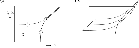
Figure 3: The phase diagram for $L=3$. (a) The self-dual subspace. The encircled numbers represent the four solvable critical branches; branches 1 and 4 describe the transition of the entire curves on which they are located, and branch 2 describes the transition across the whole lower left section of the diagram. The double curve marks a first-order transition. (b) The phase diagram with an additional parameter that reverses sign under duality. In the extreme limits (front and back) the model reduces to the interacting hard square model.

8 An Ising model in a field

Because the model in regime $2^{+}$ is in the universality class of the Ising model in a magnetic field, we take a special interest in this case, and collect the results in this section.

As we have already observed, we can make the identification $\{1,2,3\}=\{+,0,-\}$ to relate the heights of the dilute A₃ model to the states of a spin-1 Ising model. This particular model has the restriction that a ‘$+$’ and a ‘$-$’ spin may not be adjacent on the lattice. Because the nome $p$ breaks the up-down symmetry, it plays the role of the magnetic field. In Regime $2^{+}$ we see from Table I that the central charge of the model is $c={\textstyle{1\over 2}}$.

Using result (4.3) we can rewrite the free energy as

$$\ln\kappa(u)=2\sum_{k=-\infty}^{\infty}\int_{-\infty}^{\infty}\frac{\cosh 9\pi x\>\cosh 5\pi x\>\sinh 16\pi ux\>\sinh(15\pi-16u)x}{x\>\sinh 16\pi x\>\cosh 15\pi x}\;\mbox{e}^{32\,\mbox{\scriptsize i}\,\epsilon kx}\>dx.$$ (8.61)

The magnetisation of this Ising model can be expressed as a linear combination of the local state probabilities:

$$m\equiv\langle+\rangle-\langle-\rangle=P^{11}(1)-P^{11}(3)=R_{1}^{11}/\sqrt{2}.$$ (8.62)

Analogously, we can define a density for the spin-1 model, which is the probability that a site is occupied by a spin of either sign,

$$\rho\equiv\langle+\rangle+\langle-\rangle=P^{11}(1)+P^{11}(3)=\frac{1}{2}(1+R_{2}^{11}).$$ (8.63)

When we group the following combination of elliptic functions:

$$K=\frac{\vartheta_{1}\!\left({\textstyle{\pi\over 3}},t^{8}\right)\vartheta_{1}\!\left({\textstyle{\pi\over 4}},t^{90}\right)}{\vartheta_{1}\!\left({\textstyle{\pi\over 3}},t^{4}\right)N_{2}(r=1)}\sim\frac{1}{4\sqrt{6}}+O(t^{24})$$ (8.64)

and make some simplifications, the magnetisation and density are

$$m = 4\sqrt{3}\,t^{3}K\left\{E\left(-t^{54},t^{144}\right)E\left(-t^{90},t^{240}\right)-t^{24}E\left(-t^{18},t^{144}\right)E\left(-t^{30},t^{240}\right)\right\}$$

$$\rho = 2{\sqrt{6}}K\left\{\vartheta_{3}\left(0,t^{72}\right)\vartheta_{3}\left(0,t^{120}\right)-\vartheta_{2}\left(0,t^{72}\right)\vartheta_{2}\left(0,t^{120}\right)\right\}.$$ (8.65)

The leading order behaviour is

$$\begin{array}[]{rcccl}\ln\kappa_{\mbox{\scriptsize sing}}&\sim&&&p^{16/15}\\ &&&&\\ m&\sim&t^{3}&=&p^{1/15}\\ &&&&\\ \rho-{\textstyle{1\over 2}}&\sim&t^{24}&=&p^{8/15}\end{array}$$ (8.66)

The first two expressions both lead to the exponent $\delta=15$. The last exponent is related by scaling to the conformal weights of the energy and spin operators: $\Delta_{1,2}/(1-\Delta_{2,1})=8/15$.

9 Summary and discussion

In this paper we have considered the infinite hierarchy of dilute A models. These models, which belong to the family of dilute A-D-E models, can be viewed as spin-1 generalisations of the solid-on-solid models of Andrews, Baxter and Forrester [1]. For any integer $L\geq 2$, the dilute A model defines a $L$-state solid-on-solid model, with heights labelled by the Dynkin diagram of the classical Lie algebra A_L. At the critical point, the Boltzmann weights (3.25) of this solid-on-solid model obey the $\>\mbox{\sf Z}\mbox{\sf Z}\,_{2}$ symmetry of the underlying Dynkin diagram, but away from the critical point this symmetry is broken for odd values of $L$.

For each value of $L$ the model has four different critical branches. Two of these branches provide new realisations of the unitary minimal series and the two other branches can be viewed as the direct product of this same series and a $c={\textstyle{1\over 2}}$ model. Away from criticality the four branches yield eight distinct regimes.

For all regimes we have calculated the free energy. From this we have obtained critical exponents $\alpha$, for even $L$, and exponents $\delta$, for odd $L$. Among these results is the magnetic exponent $\delta=15$ of the Ising model.

The main part of this paper is concerned, however, with the calculation of the generalised order parameters for the symmetry-breaking models of the dilute A hierarchy. This calculation involved the evaluation of new sums-of-products identities for theta functions of the Rogers-Ramanujan type. From the resulting expressions for the order parameters we extracted a set of critical exponents $\delta_{k}$. For the models corresponding to the unitary minimal series, these exponents correspond to the diagonal conformal weights of the relevant Kac table. For the models corresponding to a direct product of a unitary minimal model and a $c={\textstyle{1\over 2}}$ model, the critical exponents yield the diagonal weights of the Kac table of the minimal model incremented by either one of the diagonal weights of the $c={\textstyle{1\over 2}}$ model.

We have not yet succeeded in computing the order parameters for the non-symmetry-breaking dilute A models, obtained for even values of $L$. In this case the Boltzmann weights no longer enjoy the diagonal property (5.5) and an additional diagonalisation is required. We hope to report on these ‘even’ members of the dilute A hierarchy in a future publication.

Another open problem is the relation between the symmetry-breaking spin-1 Ising model, corresponding to the dilute A₃ models in the regimes 2⁺ and 2^-, and the integrable field theory of the critical Ising model in a magnetic field, found by Zamolodchikov [28, 29]. As shown by Smirnov [30], Zamolodchikov’s $S$-matrix corresponds to an RSOS projection of the Izergin-Korepin R-matrix. Hence the dilute A₃ model provides a likely candidate for describing the corresponding solvable lattice model. The precise relation between Zamolodchikov’s $S$-matrix, which has a structure related to the Lie algebra E₈, and the dilute A₃ model remains, however, unclear. By studying the excitation spectrum of the dilute A models, and in particular the A₃ case, we hope to establish the connection, if present, in the near future.

Appendix A The function $H$

In this appendix we give the weights (3.25) in a form which is more suitable for considering the ordered or strong-field limit, and hence for obtaining the weight function $H$ defined in equation (5.5).

We first define the new variables

$$w=\mbox{e}^{-2\pi u/\epsilon}\quad\mbox{and}\quad x=\mbox{e}^{-2\pi\lambda/\epsilon}.$$ (A.1)

In terms of these variables, the ordered limit is given by $x\rightarrow 0$ with $w$ fixed. Using the conjugate nome expressions (C.11) of the theta functions and setting

$$E\left(u,x^{\pi/\lambda}\right)=E(u)$$ (A.2)

the Boltzmann weights in conjugate modulus parametrisation read

$$W\!\left(\begin{array}[]{cc}a&a\\ a&a\end{array}\right)=\frac{E(x^{6}w^{-1})E(x^{3}w)}{E(x^{6})E(x^{3})}+x^{3}\frac{E(w)E(x^{3}w^{-1})}{E(x^{6})E(x^{3})}$$ (A.5)

$$\hphantom{W\!\left(\begin{array}[]{cc}a&a\\ a&a\end{array}\right)}\times\left(x^{2}\frac{E(-x^{2a})E(x^{4(a+1)})E(-x^{2a-5})}{E(-x^{2(a+1)})E(x^{4a})E(-x^{2a+1})}+x^{-2}\frac{E(-x^{2a})E(x^{4(a-1)})E(-x^{2a+5})}{E(-x^{2(a-1)})E(x^{4a})E(-x^{2a-1})}\right)$$ (A.8)

$$W\!\left(\begin{array}[]{cc}a\pm 1&a\\ a&a\end{array}\right)=W\!\left(\begin{array}[]{cc}a&a\\ a&a\pm 1\end{array}\right)=\frac{g_{a}}{g_{a\pm 1}}w\frac{E(x^{3}w^{-1})E(-x^{\pm 2a+1}w^{-1})}{E(x^{3})E(-x^{\pm 2a+1})}$$ (A.13)

$$W\!\left(\begin{array}[]{cc}a&a\\ a\pm 1&a\end{array}\right)=W\!\left(\begin{array}[]{cc}a&a\pm 1\\ a&a\end{array}\right)$$ (A.18)

$$\hphantom{W\!\left(\begin{array}[]{cc}a&a\\ a\pm 1&a\end{array}\right)}=\frac{g_{a\pm 1}}{g_{a}}w^{-1}x^{3}\left(-x^{\mp 1}\frac{E(-x^{2a})E(x^{4(a\pm 1)})}{E(-x^{2(a\pm 1)})E(x^{4a})}\right)^{1/2}\frac{E(w)E(-x^{\pm 2a-2}w)}{E(x^{3})E(-x^{\pm 2a+1})}$$ (A.21)

$$W\!\left(\begin{array}[]{cc}a&a\pm 1\\ a&a\pm 1\end{array}\right)=W\!\left(\begin{array}[]{cc}a\pm 1&a\pm 1\\ a&a\end{array}\right)$$ (A.26)

$$\hphantom{W\!\left(\begin{array}[]{cc}a&a\pm 1\\ a&a\pm 1\end{array}\right)}=x\left(\frac{E(-x^{\pm 2a+3})E(-x^{\pm 2a-1})}{E^{2}(-x^{\pm 2a+1})}\right)^{1/2}\frac{E(w)E(x^{3}w^{-1})}{E(x^{2})E(x^{3})}$$ (A.29)

$$W\!\left(\begin{array}[]{cc}a\pm 1&a\\ a&a\mp 1\end{array}\right)=\frac{g_{a}^{2}}{g_{a+1}g_{a-1}}w\frac{E(x^{2}w^{-1})E(x^{3}w^{-1})}{E(x^{2})E(x^{3})}$$ (A.32)

$$W\!\left(\begin{array}[]{cc}a&a\mp 1\\ a\pm 1&a\end{array}\right)=-\frac{g_{a+1}g_{a-1}}{g_{a}^{2}}x^{2}\left(\frac{E^{2}(-x^{2a})E(x^{4(a-1)})E(x^{4(a+1)})}{E(-x^{2(a+1)})E(-x^{2(a-1)})E^{2}(x^{4a})}\right)^{1/2}\frac{E(w)E(xw^{-1})}{E(x^{2})E(x^{3})}$$ (A.35)

$$W\!\left(\begin{array}[]{cc}a&a\pm 1\\ a\pm 1&a\end{array}\right)=\frac{g_{a\pm 1}^{2}}{g_{a}^{2}}\frac{E(x^{3}w^{-1})E(x^{\pm 4a+2}w)}{E(x^{3})E(x^{\pm 4a+2})}$$ (A.38)

$$\hphantom{W\!\left(\begin{array}[]{cc}a&a\pm 1\\ a\pm 1&a\end{array}\right)}-\frac{g_{a\pm 1}^{2}}{g_{a}^{2}}w^{-1}x^{3\mp 1}\frac{E(-x^{2a})E(x^{4(a\pm 1)})E(w)E(x^{\pm 4a-1}w)}{E(-x^{2(a\pm 1)})E(x^{4a})E(x^{3})E(x^{\pm 4a+2})}$$ (A.41)

$$\hphantom{W\!\left(\begin{array}[]{cc}a&a\pm 1\\ a\pm 1&a\end{array}\right)}=\frac{g_{a\pm 1}^{2}}{g_{a}^{2}}w^{-1}\frac{E(x^{3}w)E(x^{\pm 4a-4}w)}{E(x^{3})E(x^{\pm 4a-4})}-\frac{g_{a\pm 1}^{2}}{g_{a}^{2}}w^{-1}\frac{E(w)E(x^{\pm 4a-1}w)}{E(x^{3})E(x^{\pm 4a-4})}$$ (A.44)

$$\hphantom{W\!\left(\begin{array}[]{cc}a&a\pm 1\\ a\pm 1&a\end{array}\right)}\times\left(x^{\pm 1-1}\frac{E(-x^{2a})E(x^{4(a\mp 1)})E(x^{4})}{E(-x^{2(a\mp 1)}E(x^{4a})E(x^{2})}+x^{3}\frac{E(-x^{\pm 2a-5})}{E(-x^{\pm 2a+1})}\right)$$ (A.47)

where we have omitted an overall normalisation factor $\exp(2u(3\lambda-u)/\epsilon)$ and $g_{a}$ is defined in equation (5.6). In this alternative representation of the Boltzmann weights, we can readily extract their leading behaviour in the ordered limit. To do so, we make use of the simple properties of the function $E$ as listed in equation (C.4) of appendix C. It is clear from the definition of $x$ that the result depends on the value of $\lambda$. For regime $1^{+}$, using definition (5.25), we get

$$H(b,b,b) = \left\{\begin{array}[]{ll}0&\quad b\in s_{1}\\ 0&\quad b\in s_{2}\\ 1&\quad b\in s_{3}\\ 1&\quad b\in s_{4}\end{array}\right.$$ (A.52)

$$H(b+1,b,b)=H(b,b,b+1) = \left\{\begin{array}[]{ll}\frac{1}{2}(b+1)&\quad b\in s_{1}\\ \frac{1}{2}b&\quad b\in s_{2}\\ \frac{1}{2}(b+2)&\quad b\in s_{3}\\ \frac{1}{2}(b+1)&\quad b\in s_{4}\setminus\{L\}\end{array}\right.$$ (A.57)

$$H(b-1,b,b)=H(b,b,b-1) = \left\{\begin{array}[]{ll}-\frac{1}{2}(b-1)&\quad b\in s_{1}\setminus\{1\}\\ -\frac{1}{2}(b-2)&\quad b\in s_{2}\\ -\frac{1}{2}(b-2)&\quad b\in s_{3}\\ -\frac{1}{2}(b-3)&\quad b\in s_{4}\end{array}\right.$$ (A.62)

$$H(b+1,b,b+1) = \left\{\begin{array}[]{ll}b+1&\quad b\in s_{1}\\ b&\quad b\in s_{2}\\ b+1&\quad b\in s_{3}\\ b+1&\quad b\in s_{4}\setminus\{L\}\end{array}\right.$$ (A.68)

$$H(b-1,b,b-1) = \left\{\begin{array}[]{ll}-(b-1)&\quad b\in s_{1}\setminus\{1\}\\ -(b-2)&\quad b\in s_{2}\\ -(b-2)&\quad b\in s_{3}\\ -(b-2)&\quad b\in s_{4}\end{array}\right.$$ (A.73)

$$H(b\pm 1,b,b\mp 1) = \begin{array}[]{ll}1&\quad b\in\{2,3,\ldots,L-1\}\end{array}.$$ (A.75)

To facilitate the proof of solution (5.26) we include the following two terms to the above list: $H(0,1,1)=0$ and $H(L+1,L,L)=\frac{1}{2}(L+1)$.

For regime $2^{+}$, using definition (5.35), we get

$$H(b,b,b) = \left\{\begin{array}[]{ll}0&\quad b\in t_{1}\\ 0&\quad b\in t_{2}\\ 1&\quad b\in t_{3}\\ 1&\quad b\in t_{4}\end{array}\right.$$ (A.80)

$$H(b+1,b,b)=H(b,b,b+1) = \left\{\begin{array}[]{ll}\frac{1}{2}(b+1)&\quad b\in t_{1}\\ \frac{1}{2}(b+2)&\quad b\in t_{2}\\ \frac{1}{2}(b+2)&\quad b\in t_{3}\\ \frac{1}{2}(b+3)&\quad b\in t_{4}\setminus\{L\}\end{array}\right.$$ (A.85)

$$H(b-1,b,b)=H(b,b,b-1) = \left\{\begin{array}[]{ll}-\frac{1}{2}(b-1)&\quad b\in t_{1}\setminus\{1\}\\ -\frac{1}{2}b&\quad b\in t_{2}\\ -\frac{1}{2}(b-2)&\quad b\in t_{3}\\ -\frac{1}{2}(b-1)&\quad b\in t_{4}\end{array}\right.$$ (A.90)

$$H(b+1,b,b+1) = \left\{\begin{array}[]{ll}b+1&\quad b\in t_{1}\\ b+2&\quad b\in t_{2}\\ b+2&\quad b\in t_{3}\\ b+2&\quad b\in t_{4}\setminus\{L\}\end{array}\right.$$ (A.96)

$$H(b-1,b,b-1) = \left\{\begin{array}[]{ll}-(b-1)&\quad b\in t_{1}\setminus\{1\}\\ -b&\quad b\in t_{2}\\ -(b-1)+\delta_{b,2}&\quad b\in t_{3}\\ -(b-1)&\quad b\in t_{4}\end{array}\right.$$ (A.101)

$$H(b\pm 1,b,b\mp 1) = \begin{array}[]{ll}1&\quad b\in\{2,\ldots,L-1\}\end{array}.$$ (A.103)

Now we only add the single term $H(0,1,1)=0$.

Appendix B Denominator identities

In this appendix we prove the six denominator identities used in section 5.4 to normalise the local height probabilities. All identities involve sums over products of elliptic functions similar to the sums-of-products identities of Rogers and Ramanujan.

For brevity we shall adopt the convention that sums over $j,k,l,m$ and $n$ always run over  ZZ .

B.1 Regime 1⁺

For regime 1⁺ the denominator identity reads

$$N_{1}\equiv\sum_{a=0}^{2L+1}\vartheta_{1}\!\left({\textstyle{a\pi\over L+1}},t^{6L(L+2)}\right)\vartheta_{3}\!\left({\textstyle{a\pi L\over 2(L+1)}},t^{3L(L+2)}\right)\vartheta_{3}\!\left({\textstyle{\pi\over 2}}\left({\textstyle{a\over L+1}}\!-\!{\textstyle{s\over L+2}}\right),t\right)$$ (B.1)

$$\hphantom{N_{1}}=2(L+1)\,t^{L(2L+3)/2}Q\left(t^{12L(L+2)}\right)Q\left(t^{12L(L+1)}\right)\vartheta_{1}\!\left({\textstyle{\pi\over 6}},t^{2(L+1)(L+2)}\right)\frac{\vartheta_{1}\!\left({\textstyle{2s\pi\over L+2}},t^{6L(L+1)}\right)}{\vartheta_{2}\!\left({\textstyle{s\pi\over L+2}},t^{6L(L+1)}\right)}$$

where $s=1,3,5,\ldots,L$ and $L=3,5,7,\ldots$.

Proof: To prove this identity we start by recasting the the left-hand side using the representation (C.1) of the $\vartheta$-functions as infinite sums:

$$N_{1}=-\,\mbox{i}\,t^{3L(L+2)/2}\sum_{a=0}^{2L+1}\sum_{j,k,\ell}(-1)^{j}\,\mbox{e}^{\pi\,\mbox{\scriptsize i}\,a(2j+1+kL+\ell)/(L+1)}\,\mbox{e}^{-\pi\,\mbox{\scriptsize i}\,s\ell/(L+2)}$$ (B.2)

$$\qquad\qquad\qquad\qquad\qquad\qquad\times\>\vphantom{\sum^{a}}t^{6L(L+2)(j^{2}+j)+3L(L+2)k^{2}+\ell^{2}}.$$

Summing the roots of unity over $a$, we find that the above expression vanishes unless $\ell=-2j-1-kL+2m(L+1)$, with $m\in\>\mbox{\sf Z}\mbox{\sf Z}\,$. Hence we get

$$N_{1}=-2\,\mbox{i}\,(L+1)\,t^{3L(L+2)/2}\sum_{j,k,m}(-1)^{j+k}\,\mbox{e}^{\pi\,\mbox{\scriptsize i}\,s(2j+1-2k+2m)/(L+2)}$$ (B.3)

$$\qquad\qquad\qquad\qquad\qquad\qquad\times\>\vphantom{\sum^{a}}t^{6L(L+2)(j^{2}+j)+3L(L+2)k^{2}+[2j+1+kL-2m(L+1)]^{2}}$$

where we have used the fact that $s$ is odd.

We now carry out a sequence of transformations to diagonalise the quadratic exponent of $t$. First we make the substitution $m\to m-j+k$ followed by $k\to k+2j$. Then we replace the sum over $k$ by a sum over $\ell$ and $\alpha$ by setting $k=3\ell+\alpha$, where $\alpha$ has to be summed over $0,1$ and 2. Similarly, we replace the sum over $m$ by a sum over $n$ and $\beta$ by setting $m=3n+\beta$. Finally we make the replacements $j\to j-\ell$ and $\ell\to\ell-n$. After all these transformations we obtain

$$N_{1}=-2\,\mbox{i}\,(L+1)\,t^{(3L^{2}+6L+2)/2}\sum_{\alpha,\beta=0}^{2}\sum_{j,\ell,n}(-1)^{j+\alpha}\,\mbox{e}^{\pi\,\mbox{\scriptsize i}\,s(6n+2\beta+1)/(L+2)}$$

$$\quad\qquad\times\>t^{4(\alpha+\beta)(\alpha+\beta-1)+2L(5\alpha^{2}+4\beta^{2}+6\alpha\beta-\alpha-2\beta)+4L^{2}(\alpha^{2}+\beta^{2}+\alpha\beta)}\vphantom{\sum_{a}^{a}}$$

$$\quad\qquad\times\>t^{6L(L+2)(3j+1+2\alpha)j+6(L+1)(L+2)(3\ell-1+2\alpha+2\beta)\ell+6L(L+1)(3n+1+2\beta)n}\vphantom{\sum_{a}^{a}}$$

$$\hphantom{N_{1}}=-2\,\mbox{i}\,(L+1)\,t^{(3L^{2}+6L+2)/2}$$

$$\qquad\quad\times\sum_{\alpha,\beta=0}^{2}(-1)^{\alpha}\,t^{4(\alpha+\beta)(\alpha+\beta-1)+2L(5\alpha^{2}+4\beta^{2}+6\alpha\beta-\alpha-2\beta)+4L^{2}(\alpha^{2}+\beta^{2}+\alpha\beta)}$$

$$\qquad\quad\times\>\mbox{e}^{\pi\,\mbox{\scriptsize i}\,s(2\beta+1)/(L+2)}E\!\left(-\mbox{e}^{6\pi\,\mbox{\scriptsize i}\,s/(L+2)}\,t^{12L(L+1)(2+\beta)},t^{36L(L+1)}\right)\vphantom{\sum_{a}^{a}}$$

$$\qquad\quad\times\>E\!\left(t^{12L(L+2)(2+\alpha)},t^{36L(L+2)}\right)E\!\left(-t^{12(L+1)(L+2)(1+\alpha+\beta)},t^{36(L+1)(L+2)}\right).\vphantom{\sum^{a}}$$

where, in the second step, we have used the definition (C.3) of the function $E$. The terms with $\alpha=1$ are identically zero and the two terms with $\beta=1$, $\alpha\neq 1$ cancel. The remaining four terms factorise to give

$$N_{1}=2\,\mbox{i}\,(L+1)\,t^{(3L^{2}+6L+2)/2}\,\mbox{e}^{-\pi\,\mbox{\scriptsize i}\,s/(L+2)}Q\left(t^{12L(L+2)}\right)\vphantom{\sum_{a}}$$

$$\qquad\qquad\times\!\left[E\!\left(-t^{12(L+1)(L+2)},t^{36(L+1)(L+2)}\right)-t^{4(L+1)(L+2)}E\!\left(-1,t^{36(L+1)(L+2)}\right)\right]\vphantom{\sum_{a}^{a}}$$

$$\qquad\qquad\times\!\left[E\!\left(-\mbox{e}^{6\pi\,\mbox{\scriptsize i}\,s/(L+2)}\,t^{12L(L+1)},t^{36L(L+1)}\right)\right.\vphantom{\sum_{a}^{a}}$$ (B.5)

$$\qquad\qquad\qquad\qquad\qquad\qquad\left.-\mbox{e}^{2\pi\,\mbox{\scriptsize i}\,s/(L+2)}E\!\left(-\mbox{e}^{-6\pi\,\mbox{\scriptsize i}\,s/(L+2)}\,t^{12L(L+1)},t^{36L(L+1)}\right)\right].\vphantom{\sum^{a}}$$

We now note the following two elliptic function identities:

$$\vphantom{\sum_{a}^{a}}E\left(-x^{3}p,p^{3}\right)-xE\left(-x^{-3}p,p^{3}\right)=\frac{Q(p)\,E\left(x^{2},p\right)}{E\left(-x,p\right)}$$

$$\vphantom{\sum_{a}^{a}}E\left(-p^{3},p^{9}\right)-pE\left(-1,p^{9}\right)=\mbox{e}^{\pi\,\mbox{\scriptsize i}\,/3}E\left(\mbox{e}^{\pi\,\mbox{\scriptsize i}\,/3},p\right).$$ (B.6)

To prove the first identity we note that the function $f(x)$, defined as the ratio of the left-hand side over the right-hand side, has the following periodicity property: $f(px)=f(x)$. Since the function $E(x,p)$ is analytic in $0<|x|<\infty$, the only possible poles in the period annulus $p\leq|x|\leq 1$ are the zeros $x=\pm 1$ and $x=\pm p^{1/2}$ of the function $E(x^{2},p)$. Using formula (C.4) to manipulate the function $E$ it is readily verified that these poles have zero residue. Hence, by Liouville’s theorem, $f$ is constant. Setting $x=-p^{1/3}$ shows that this constant is one. The second identity is actually a corollary of the first. Replacing $p$ by $p^{3}$, then setting $x=p^{2}$ and again using formula (C.4), yields

$$E\left(-p^{3},p^{9}\right)-pE\left(-1,p^{9}\right)=-p\>\frac{E\left(p^{4},p^{3}\right)Q\left(p^{3}\right)}{E\left(-p^{2},p^{3}\right)}$$

$$\hphantom{E\left(-p^{3},p^{9}\right)-pE\left(-1,p^{9}\right)}=\prod_{n=1}^{\infty}\left(1-p^{n}+p^{2n}\right)$$ (B.7)

$$\hphantom{E\left(-p^{3},p^{9}\right)-pE\left(-1,p^{9}\right)}=\mbox{e}^{\pi\,\mbox{\scriptsize i}\,/3}E\left(\mbox{e}^{\pi\,\mbox{\scriptsize i}\,/3},p\right).\vphantom{\sum^{a}}$$

Applying both identities and the relation (C.9) of appendix C, we obtain the desired right-hand side of (B.1).

B.2 Regime 2⁺

For regime 2⁺ we have to prove the following identity:

$$N_{2}\equiv\sum_{a=0}^{2L+1}\vartheta_{1}\!\left({\textstyle{a\pi\over L+1}},t^{6L(L+2)}\right)\vartheta_{3}\!\left({\textstyle{a\pi L\over 2(L+1)}},t^{3L(L+2)}\right)\vartheta_{3}\!\left({\textstyle{\pi\over 2}}\left({\textstyle{r\over L}}\!-\!{\textstyle{a\over L+1}}\right),t\right)$$ (B.8)

$$\hphantom{N_{2}}=2(L\!+\!1)t^{(L+2)(2L+1)/2}Q\left(t^{12L(L+2)}\right)Q\left(t^{12(L+1)(L+2)}\right)\vartheta_{1}\!\left({\textstyle{\pi\over 6}},t^{2L(L+1)}\right)\frac{\vartheta_{1}\!\left({\textstyle{2r\pi\over L}},t^{6(L+1)(L+2)}\right)}{\vartheta_{2}\!\left({\textstyle{r\pi\over L}},t^{6(L+1)(L+2)}\right)}$$

where $r=1,3,5,\ldots,L-2$ and $L=3,5,7,\ldots$.

Proof: The proof of this denominator identity is similar to that presented for regime 1⁺. Using the representation of the $\vartheta$-functions as infinite sums yields

$$N_{2}=-\,\mbox{i}\,t^{3L(L+2)/2}\sum_{a=0}^{2L+1}\sum_{j,k,\ell}(-1)^{j}\mbox{e}^{\pi\,\mbox{\scriptsize i}\,a(2j+1+kL-\ell)/(L+1)}\mbox{e}^{\pi\,\mbox{\scriptsize i}\,r\ell/L}t^{6L(L+2)(j^{2}+j)+3L(L+2)k^{2}+\ell^{2}}\!.$$ (B.9)

Performing the sum over $a$ gives $\ell=2j+1+kL+2m(L+1)$, where $m$ assumes integer values. Thus we find

$$N_{2}=-2\,\mbox{i}\,(L+1)\,t^{3L(L+2)/2}\sum_{j,k,m}(-1)^{j+k}\,\mbox{e}^{\pi\,\mbox{\scriptsize i}\,r(2j+1+2m)/L}$$ (B.10)

$$\qquad\qquad\qquad\qquad\qquad\qquad\times\>\vphantom{\sum^{a}}t^{6L(L+2)L(j^{2}+j)+3L(L+2)k^{2}+[2j+1+kL+2m(L+1)]^{2}}$$

where we have used the fact that $r$ is odd.

As before, we carry out a sequence of transformations to diagonalise the quadratic exponent of $t$. First we make the replacements $m\to m-j$ and $k\to k+2j$. Then we set $k=3\ell+\alpha$ and $m=3n+\beta$ and finally we substitute $j\to j-\ell$ followed by $\ell\to\ell-n$. After making these transformations we obtain

$$N_{2}=-2\,\mbox{i}\,(L+1)\,t^{(3L^{2}+6L+2)/2}\sum_{\alpha,\beta=0}^{2}(-1)^{\alpha}\,t^{4\beta(\beta+1)+2L(3\alpha^{2}+4\beta^{2}+2\alpha\beta+\alpha+2\beta)+4L^{2}(\alpha^{2}+\beta^{2}+\alpha\beta)}$$

$$\qquad\quad\times\>\mbox{e}^{\pi\,\mbox{\scriptsize i}\,r(2\beta+1)/L}E\!\left(-\mbox{e}^{6\pi\,\mbox{\scriptsize i}\,r/L}\,t^{12(L+1)(L+2)(2+\beta)},t^{36(L+1)(L+2)}\right)\vphantom{\sum_{a}^{a}}$$

$$\qquad\quad\times\>E\!\left(t^{12L(L+2)(2+\alpha)},t^{36L(L+2)}\right)E\!\left(-t^{12L(L+1)(1+\alpha+\beta)},t^{36L(L+1)}\right).\vphantom{\sum^{a}}$$

The terms with $\alpha=1$ vanish and the terms with $\beta=1$ cancel. The remaining four terms can be written as

$$N_{2}=2\,\mbox{i}\,(L+1)\,t^{(3L^{2}+6L+2)/2}\,\mbox{e}^{-\pi\,\mbox{\scriptsize i}\,r/L}Q\left(t^{12L(L+2)}\right)\vphantom{\sum_{a}}$$

$$\qquad\qquad\times\!\left[E\!\left(-t^{12L(L+1)},t^{36L(L+1)}\right)-t^{4L(L+1)}E\!\left(-1,t^{36L(L+1)}\right)\right]\vphantom{\sum_{a}^{a}}$$ (B.12)

$$\qquad\qquad\times\!\left[E\!\left(-\mbox{e}^{6\pi\,\mbox{\scriptsize i}\,r/L}\,t^{12(L+1)(L+2)},t^{36(L+1)(L+2)}\right)\right.\vphantom{\sum_{a}^{a}}$$

$$\qquad\qquad\qquad\qquad\qquad\qquad\left.-\mbox{e}^{2\pi\,\mbox{\scriptsize i}\,r/L}E\!\left(-\mbox{e}^{-6\pi\,\mbox{\scriptsize i}\,r/L}\,t^{12(L+1)(L+2)},t^{36(L+1)(L+2)}\right)\right].\vphantom{\sum^{a}}$$

If we again apply the two identities of equation (B.6) and use the relation (C.9), we obtain the required right-hand side of equation (B.8).

B.3 Regime 3⁺

Antiferromagnetic phase

For the antiferromagnetic phases of regime 3⁺ the denominator identity is given by

$$N_{3}\equiv\sum_{a=0}^{2L+1}\vartheta_{3}\!\left({\textstyle{(1+2\mu_{a})\pi\over 8}},t^{(L+1)(L+2)/4}\right)\vartheta_{1}\!\left({\textstyle{a\pi\over L+1}},t^{2(L^{2}-4)}\right)\vartheta_{3}\!\left({\textstyle{a\pi L\over 2(L+1)}},t^{L^{2}-4}\right)\vartheta_{3}\!\left({\textstyle{\pi\over 2}}\left({\textstyle{a\over L+1}}\!-\!{\textstyle{s\over L+2}}\right),t\right)$$

$$\hphantom{N_{3}}=2(L+1)\,t^{(L-1)(L+2)/4}Q\left(t^{4(L^{2}-4)}\right)Q\left(t^{2(L+1)(L+2)}\right)$$ (B.13)

$$\qquad\qquad\qquad\qquad\qquad\qquad\qquad\qquad\quad\times\vartheta_{3}\!\left({\textstyle{\pi\over 4}},t^{(L+1)(L+2)}\right)\vartheta_{1}\!\left({\textstyle{s\pi\over L+2}},t^{(L+1)(L-2)}\right)$$

where $\mu_{a}=a+\sigma\bmod 2$ with $\sigma=0,1$; $s=1,3,5,\ldots,L$ and $L=3,5,7,\ldots$.

Proof: We split the summation on the left-hand side depending on the parity of $a$. Using the fact that $\vartheta_{3}(u+{\textstyle{1\over 2}}\pi,p)=\vartheta_{4}(u,p)=\vartheta_{3}(u,-p)$, we get

$$N_{3}=\vartheta_{3}\!\left({\textstyle{\pi\over 8}},(-1)^{\sigma}t^{(L+1)(L+2)/4}\right)\sum_{a=0}^{L}\vartheta_{1}\!\left({\textstyle{2a\pi\over L+1}},t^{2(L^{2}-4)}\right)\vartheta_{3}\!\left({\textstyle{a\pi L\over L+1}},t^{L^{2}-4}\right)\vartheta_{3}\!\left({\textstyle{\pi\over 2}}\left({\textstyle{2a\over L+1}}\!-\!{\textstyle{s\over L+2}}\right),t\right)$$

$$\hphantom{N_{3}}+\vartheta_{3}\!\left({\textstyle{3\pi\over 8}},(-1)^{\sigma}t^{(L+1)(L+2)/4}\right)\sum_{a=0}^{L}\vartheta_{1}\!\left({\textstyle{(2a+1)\pi\over L+1}},t^{2(L^{2}-4)}\right)$$ (B.14)

$$\qquad\qquad\qquad\qquad\qquad\qquad\qquad\qquad\times\>\vartheta_{3}\!\left({\textstyle{(2a+1)\pi L\over 2(L+1)}},t^{L^{2}-4}\right)\vartheta_{3}\!\left({\textstyle{\pi\over 2}}\left({\textstyle{2a+1\over L+1}}\!-\!{\textstyle{s\over L+2}}\right),t\right).$$

We now represent the theta-functions with $a$-dependent arguments by series to obtain

$$N_{3}=-\,\mbox{i}\,t^{(L^{2}-4)/2}\sum_{a=0}^{L}\sum_{j,k,\ell}(-1)^{j}\,\mbox{e}^{2\pi\,\mbox{\scriptsize i}\,a(2j+1+kL+\ell)/(L+1)}\,\mbox{e}^{-\pi\,\mbox{\scriptsize i}\,s\ell/(L+2)}\,t^{(L^{2}-4)(2j^{2}+2j+k^{2})+\ell^{2}}$$

$$\vphantom{\sum^{a}}\qquad\times\left[\vartheta_{3}\!\left({\textstyle{\pi\over 8}},(-1)^{\sigma}t^{(L+1)(L+2)/4}\right)+\mbox{e}^{\pi\,\mbox{\scriptsize i}\,(2j+1+kL+\ell)/(L+1)}\vartheta_{3}\!\left({\textstyle{3\pi\over 8}},(-1)^{\sigma}t^{(L+1)(L+2)/4}\right)\right].$$ (B.15)

Performing the sum over $a$, we find that $\ell=-2j-1-kL+m(L+1)$ and hence

$$N_{3}=-\,\mbox{i}\,(L+1)\,t^{(L^{2}-4)/2}\sum_{j,k,m}(-1)^{j+k}\,\mbox{e}^{\pi\,\mbox{\scriptsize i}\,s(2j+1-2k+m)/(L+2)}$$

$$\qquad\qquad\quad\times\>\vphantom{\sum_{a}^{a}}t^{(L^{2}-4)(2j^{2}+2j+k^{2})+[2j+1+kL-m(L+1)]^{2}}$$

$$\qquad\qquad\quad\times\>\left[(-1)^{m}\vartheta_{3}\!\left({\textstyle{\pi\over 8}},(-1)^{\sigma}t^{(L+1)(L+2)/4}\right)+\vartheta_{3}\!\left({\textstyle{3\pi\over 8}},(-1)^{\sigma}t^{(L+1)(L+2)/4}\right)\right]$$

where we have used the fact that $s$ is odd.

Again we carry out a sequence of transformations to diagonalise the quadratic exponent of $t$. First we make the replacements $m\to m-2j+2k$ and $k\to k+2j$, followed by the substitutions $k=3\ell+\alpha$ and $m=4n+\beta$. Finally we set $j\to j-\ell$ and $\ell\to\ell-n$ to obtain

$$N_{3}=-\,\mbox{i}\,(L+1)\,t^{(L^{2}-2)/2}\sum_{\alpha=0}^{2}\sum_{\beta=0}^{3}(-1)^{\alpha}\,t^{\beta^{2}+4\alpha\beta-4\alpha-2\beta+2L(2\alpha^{2}+\beta^{2}+3\alpha\beta-\alpha-\beta)+L^{2}(2\alpha^{2}+\beta^{2}+2\alpha\beta)}$$

$$\quad\qquad\times\left[(-1)^{\beta}\vartheta_{3}\!\left({\textstyle{\pi\over 8}},(-1)^{\sigma}t^{(L+1)(L+2)/4}\right)+\vartheta_{3}\!\left({\textstyle{3\pi\over 8}},(-1)^{\sigma}t^{(L+1)(L+2)/4}\right)\right]\vphantom{\sum_{a}^{a}}$$

$$\quad\qquad\times\>\mbox{e}^{\pi\,\mbox{\scriptsize i}\,s(\beta+1)/(L+2)}E\!\left(-\mbox{e}^{4\pi\,\mbox{\scriptsize i}\,s/(L+2)}\,t^{2(L+1)(L-2)(3+\beta)},t^{8(L+1)(L-2)}\right)\vphantom{\sum_{a}^{a}}$$

$$\quad\qquad\times\>E\!\left(t^{4(L^{2}-4)(2+\alpha)},t^{12(L^{2}-4)}\right)E\!\left(-t^{2(L+1)(L+2)(5+4\alpha+3\beta)},t^{24(L+1)(L+2)}\right).\vphantom{\sum^{a}}$$

In this expression the terms with $\alpha=1$ vanish and the terms with $\beta=1$ and $\beta=3$ cancel. Using the simple identity

$$\vartheta_{3}\!\left({\textstyle{\pi\over 8}},p\right)+\vartheta_{3}\!\left({\textstyle{3\pi\over 8}},p\right)=2\vartheta_{3}\!\left({\textstyle{\pi\over 4}},p^{4}\right)$$ (B.18)

which follows directly from (C.1), the remaining four terms factorise as

$$\vphantom{\sum_{a}}N_{3}=2\,\mbox{i}\,(L+1)\,\mbox{e}^{-\pi\,\mbox{\scriptsize i}\,s/(L+2)}\,t^{(L^{2}-2)/2}Q\left(t^{4(L^{2}-4)}\right)\vartheta_{3}\!\left({\textstyle{\pi\over 4}},t^{(L+1)(L+2)}\right)$$

$$\vphantom{\sum_{a}^{a}}\qquad\times\left[E\!\left(-t^{10(L+1)(L+2)},t^{24(L+1)(L+2)}\right)-t^{2(L+1)(L+2)}E\!\left(-t^{2(L+1)(L+2)},t^{24(L+1)(L+2)}\right)\right]$$

$$\vphantom{\sum_{a}^{a}}\qquad\times\left[E\!\left(-\mbox{e}^{4\pi\,\mbox{\scriptsize i}\,s/(L+2)}\,t^{2(L+1)(L-2)},t^{8(L+1)(L-2)}\right)\right.$$ (B.19)

$$\vphantom{\sum_{a}^{a}}\qquad\qquad\qquad\qquad\qquad\qquad\left.-\mbox{e}^{2\pi\,\mbox{\scriptsize i}\,s/(L+2)}E\!\left(-\mbox{e}^{-4\pi\,\mbox{\scriptsize i}\,s/(L+2)}\,t^{2(L+1)(L-2)},t^{8(L+1)(L-2)}\right)\right].$$

We now note the identities

$$\vphantom{\sum_{a}^{a}}E\left(-x^{2}p,p^{4}\right)-xE\left(-x^{-2}p,p^{4}\right)=E\left(x,p\right)$$

$$\vphantom{\sum^{a}}E\left(-p^{5},p^{12}\right)-pE\left(-p,p^{12}\right)=Q(p).$$ (B.20)

The first one follows directly from Liouville’s theorem and the second one can be obtained from the first upon setting $x=p$ after replacing $p$ by $p^{3}$. If we apply these two identities, as well as equation (C.9), we find precisely the right-hand side of equation (B.13). This completes the proof.

Ferromagnetic phase

The denominator identity for the ferromagnetic phases in regime 3⁺ reads

$$N_{4}\equiv\sum_{a=0}^{2L+1}\vartheta_{1}\!\left({\textstyle{a\pi\over L+1}},t^{2(L^{2}-4)}\right)\vartheta_{3}\!\left({\textstyle{a\pi L\over 2(L+1)}},t^{L^{2}-4}\right)\vartheta_{3}\!\left({\textstyle{\pi\over 2}}\left({\textstyle{a\over L+1}}\!-\!{\textstyle{s\over L+2}}\right),t\right)$$ (B.21)

$$\hphantom{N_{4}}=4(L\!+\!1)t^{L(L+2)/2}Q^{2}\!\left(t^{4(L+1)(L+2)}\right)Q\!\left(t^{4(L^{2}-4)}\right)\frac{\vartheta_{1}\!\left({\textstyle{s\pi\over L+2}},t^{2(L+1)(L-2)}\right)\vartheta_{3}\!\left({\textstyle{s\pi\over L+2}},t^{2(L+1)(L-2)}\right)}{\vartheta_{1}\!\left({\textstyle{\pi\over 4}},t^{(L+1)(L-2)}\right)\vartheta_{1}\!\left({\textstyle{\pi\over 4}},t^{(L+1)(L+2)}\right)}$$

where $s=2,4,6,\ldots,L+1$ and $L=3,5,7,\ldots$.

Proof: We begin by writing the sum over the $\vartheta$-functions in the left-hand side as

$$N_{4}=-\,\mbox{i}\,t^{(L^{2}-4)/2}\sum_{a=0}^{2L+1}\sum_{j,k,\ell}(-1)^{j}\,\mbox{e}^{\pi\,\mbox{\scriptsize i}\,a(2j+1+kL+\ell)/(L+1)}\,\mbox{e}^{-\pi\,\mbox{\scriptsize i}\,s\ell/(L+2)}\,t^{(L^{2}-4)(2j^{2}+2j+k^{2})+\ell^{2}}.$$ (B.22)

Summing over $a$ yields $\ell=-2j-1-kL+2m(L+1)$ and hence, using the fact that $s$ is even, we get

$$N_{4}=-2\,\mbox{i}\,(L+1)\,t^{(L^{2}-4)/2}\sum_{j,k,m}(-1)^{j}\,\mbox{e}^{\pi\,\mbox{\scriptsize i}\,s(2j+1-2k+2m)/(L+2)}$$ (B.23)

$$\qquad\qquad\qquad\qquad\qquad\qquad\times\>\vphantom{\sum^{a}}t^{(L^{2}-4)(2j^{2}+2j+k^{2})+[2j+1+kL-2m(L+1)]^{2}}.$$

In order to diagonalise the quadratic exponent of $t$, we make the replacements $m\to m-j+k$ and $k\to k+2j$ followed by the substitutions $k=3\ell+\alpha$ and $m=2n+\beta$. Further replacing $j\to j-\ell$ and $\ell\to\ell-n$ leads to the result

$$N_{4}=-2\,\mbox{i}\,(L+1)\,t^{(L^{2}-2)/2}\sum_{\alpha=0}^{2}\sum_{\beta=0}^{1}t^{4(\beta^{2}+2\alpha\beta-\alpha-\beta)+2L(2\alpha^{2}+4\beta^{2}+6\alpha\beta-\alpha-2\beta)+2L^{2}(\alpha^{2}+2\beta^{2}+2\alpha\beta)}$$

$$\vphantom{\sum_{a}^{a}}\qquad\qquad\times\mbox{e}^{\pi\,\mbox{\scriptsize i}\,s(2\beta+1)/(L+2)}E\!\left(\mbox{e}^{4\pi\,\mbox{\scriptsize i}\,s/(L+2)}\,t^{2(L+1)(L-2)(3+2\beta)},t^{8(L+1)(L-2)}\right)$$ (B.24)

$$\qquad\vphantom{\sum_{a}^{a}}\qquad\times E\!\left(t^{4(L^{2}-4)(2+\alpha)},t^{12(L^{2}-4)}\right)E\!\left(t^{2(L+1)(L+2)(5+4\alpha+6\beta)},t^{24(L+1)(L+2)}\right).$$

The terms with $\alpha=1$ vanish and the other terms may be combined to give

$$\vphantom{\sum_{a}}N_{4}=2\,\mbox{i}\,(L+1)\,\mbox{e}^{-\pi\,\mbox{\scriptsize i}\,s/(L+2)}\,t^{(L^{2}-2)/2}Q\left(t^{4(L^{2}-4)}\right)$$

$$\vphantom{\sum_{a}^{a}}\qquad\times\left[E\!\left(t^{10(L+1)(L+2)},t^{24(L+1)(L+2)}\right)+t^{2(L+1)(L+2)}E\!\left(t^{2(L+1)(L+2)},t^{24(L+1)(L+2)}\right)\right]$$

$$\vphantom{\sum_{a}^{a}}\qquad\times\left[E\!\left(\mbox{e}^{4\pi\,\mbox{\scriptsize i}\,s/(L+2)}\,t^{2(L+1)(L-2)},t^{8(L+1)(L-2)}\right)\right.$$ (B.25)

$$\vphantom{\sum_{a}^{a}}\qquad\qquad\qquad\qquad\qquad\qquad\left.-\mbox{e}^{2\pi\,\mbox{\scriptsize i}\,s/(L+2)}E\!\left(\mbox{e}^{-4\pi\,\mbox{\scriptsize i}\,s/(L+2)}\,t^{2(L+1)(L-2)},t^{8(L+1)(L-2)}\right)\right].$$

If we multiply this expression with the prefactors outside the sum in equation (B.21) and use the following identities

$$\vphantom{\sum_{a}^{a}}E\left(x^{2}p,p^{4}\right)-xE\left(x^{-2}p,p^{4}\right)=\sqrt{2}\,\mbox{e}^{-\pi\,\mbox{\scriptsize i}\,/4}\>\frac{E\left(x,p^{2}\right)E\left(-xp,p^{2}\right)}{E(i,p)}$$

$$E\left(p^{5},p^{12}\right)+pE\left(p,p^{12}\right)=\sqrt{2}\,\mbox{e}^{-\pi\,\mbox{\scriptsize i}\,/4}\>\frac{Q^{2}\left(p^{2}\right)}{E(i,p)}$$ (B.26)

we find precisely the right-hand side of equation (B.21). The proof of these two relations is similar to those obtained earlier. The first identities follows from application of Liouville’s theorem and the second identity is a consequence of the first. Replacing the nome $p$ by $p^{3}$ and then setting $x=p^{2}$ yields

$$E\left(p^{5},p^{12}\right)+pE\left(p,p^{12}\right)=\sqrt{2}\,\mbox{e}^{-\pi\,\mbox{\scriptsize i}\,/4}\>Q(p^{2})\>\frac{E(-p^{5},p^{6})}{E(i,p^{3})}$$

$$\hphantom{E\left(p^{5},p^{12}\right)+pE\left(p,p^{12}\right)}=Q(p^{2})\prod_{n=1}^{\infty}\frac{\left(1+p^{6n-5}\right)\left(1+p^{6n-1}\right)\left(1+p^{3n}\right)}{\left(1+p^{6n}\right)}$$

$$\hphantom{E\left(p^{5},p^{12}\right)+pE\left(p,p^{12}\right)}=Q(p^{2})\prod_{n=1}^{\infty}\left(1+p^{2n-1}\right)$$ (B.27)

$$\hphantom{E\left(p^{5},p^{12}\right)+pE\left(p,p^{12}\right)}=\sqrt{2}\,\mbox{e}^{-\pi\,\mbox{\scriptsize i}\,/4}\>\frac{Q^{2}\left(p^{2}\right)}{E(i,p)}.$$

B.4 Regime 4⁺

Antiferromagnetic phase

The denominator identity in the antiferromagnetic phase of regime 4⁺ is given by

$$N_{5}\equiv\sum_{a=0}^{2L+1}\vartheta_{3}\!\left({\textstyle{(1+2\mu_{a})\pi\over 8}},t^{L(L+1)/4}\right)\vartheta_{1}\!\left({\textstyle{a\pi\over L+1}},t^{2L(L+4)}\right)\vartheta_{3}\!\left({\textstyle{a\pi L\over 2(L+1)}},t^{L(L+4)}\right)\vartheta_{3}\!\left({\textstyle{\pi\over 2}}\left({\textstyle{r\over L}}\!-\!{\textstyle{a\over L+1}}\right),t\right)$$

$$\hphantom{N_{5}}=2(L+1)\,t^{L(L+3)/4}Q\left(t^{4L(L+4)}\right)Q\left(t^{2L(L+1)}\right)\vartheta_{3}\!\left({\textstyle{\pi\over 4}},t^{L(L+1)}\right)\vartheta_{1}\!\left({\textstyle{r\pi\over L}},t^{(L+1)(L+4)}\right)$$ (B.28)

where $\mu_{a}=a+\sigma\bmod 2$, with $\sigma=0,1$; $r=1,3,5,\ldots,L-2$ and $L=3,5,7,\ldots$.

Proof: Following the proof for the antiferromagnetic phase of regime 3⁺, we split the summation on the left-hand side depending on the parity of $a$. Representing the theta functions with $a$-dependent arguments by series yields

$$N_{5}=-\,\mbox{i}\,t^{L(L+4)/2}\sum_{a=0}^{L}\sum_{j,k,\ell}(-1)^{j}\,\mbox{e}^{2\pi\,\mbox{\scriptsize i}\,a(2j+1+kL-\ell)/(L+1)}\,\mbox{e}^{\pi\,\mbox{\scriptsize i}\,r\ell/L}\,t^{L(L+4)(2j^{2}+2j+k^{2})+\ell^{2}}$$

$$\vphantom{\sum_{a}^{a}}\qquad\times\left[\vartheta_{3}\!\left({\textstyle{\pi\over 8}},(-1)^{\sigma}t^{L(L+1)/4}\right)+\mbox{e}^{\pi\,\mbox{\scriptsize i}\,(2j+1+kL-\ell)/(L+1)}\vartheta_{3}\!\left({\textstyle{3\pi\over 8}},(-1)^{\sigma}t^{L(L+1)/4}\right)\right].$$ (B.29)

Summing the roots of unity over $a$ we see that $\ell=2j+1+kL+m(L+1)$ and as a result we have

$$N_{5}=-\,\mbox{i}\,(L+1)\,t^{L(L+4)/2}\sum_{j,k,m}(-1)^{j+k}\,\mbox{e}^{\pi\,\mbox{\scriptsize i}\,r(2j+1+m)/L}\,t^{L(L+4)(2j^{2}+2j+k^{2})+[2j+1+kL+m(L+1)]^{2}}$$ (B.30)

$$\qquad\qquad\qquad\qquad\times\left[(-1)^{m}\vartheta_{3}\!\left({\textstyle{\pi\over 8}},(-1)^{\sigma}t^{L(L+1)/4}\right)+\vartheta_{3}\!\left({\textstyle{3\pi\over 8}},(-1)^{\sigma}t^{L(L+1)/4}\right)\right]$$

where we have used the fact that $r$ is odd.

We diagonalise the quadratic exponent of $t$ by carrying out the following sequence of replacements. We first set $m\to m-2j$ and $k\to k+2j$. We then replace $k=3\ell+\alpha$ and $m=4n+\beta$ and finally we substitute $j\to j-\ell$ followed by $\ell\to\ell-n$. We then have

$$N_{5}=-\,\mbox{i}\,(L+1)\,t^{(L^{2}+4L+2)/2}\sum_{\alpha=0}^{2}\sum_{\beta=0}^{3}(-1)^{\alpha}\,t^{\beta(\beta+2)+2L(2\alpha^{2}+\beta^{2}+\alpha\beta+\alpha+\beta)+L^{2}(2\alpha^{2}+\beta^{2}+2\alpha\beta)}$$

$$\qquad\quad\times\left[(-1)^{\beta}\vartheta_{3}\!\left({\textstyle{\pi\over 8}},(-1)^{\sigma}t^{L(L+1)/4}\right)+\vartheta_{3}\!\left({\textstyle{3\pi\over 8}},(-1)^{\sigma}t^{L(L+1)/4}\right)\right]\vphantom{\sum_{a}^{a}}$$

$$\qquad\quad\times\>\mbox{e}^{\pi\,\mbox{\scriptsize i}\,r(\beta+1)/L}E\!\left(-\mbox{e}^{4\pi\,\mbox{\scriptsize i}\,r/L}\,t^{2(L+1)(L+4)(3+\beta)},t^{8(L+1)(L+4)}\right)\vphantom{\sum_{a}^{a}}$$

$$\qquad\quad\times\>E\!\left(t^{4L(L+4)(2+\alpha)},t^{12L(L+4)}\right)E\!\left(-t^{2L(L+1)(5+4\alpha+3\beta)},t^{24L(L+1)}\right).\vphantom{\sum^{a}}$$

As before, the terms with $\alpha=1$ vanish and the terms with $\beta=1$ and $\beta=3$ cancel. Using the relation (B.18), the remaining four terms can be written as

$$\vphantom{\sum_{a}}N_{5}=2\,\mbox{i}\,(L+1)\,\mbox{e}^{-\pi\,\mbox{\scriptsize i}\,r/L}\,t^{(L^{2}+4L+2)/2}Q\left(t^{4L(L+4)}\right)\vartheta_{3}\!\left({\textstyle{\pi\over 4}},t^{L(L+1)}\right)$$

$$\qquad\qquad\times\!\left[E\!\left(-t^{10L(L+1)},t^{24L(L+1)}\right)-t^{2L(L+1)}E\!\left(-t^{2L(L+1)},t^{24L(L+1)}\right)\right]\vphantom{\sum_{a}^{a}}$$

$$\qquad\qquad\times\!\left[E\!\left(-\mbox{e}^{4\pi\,\mbox{\scriptsize i}\,r/L}\,t^{2(L+1)(L+4)},t^{8(L+1)(L+4)}\right)\right.\vphantom{\sum_{a}^{a}}$$ (B.32)

$$\qquad\qquad\qquad\qquad\qquad\qquad\left.-\mbox{e}^{2\pi\,\mbox{\scriptsize i}\,r/L}E\!\left(-\mbox{e}^{-4\pi\,\mbox{\scriptsize i}\,r/L}\,t^{2(L+1)(L+4)},t^{8(L+1)(L+4)}\right)\right].\vphantom{\sum^{a}}$$

After application of the identities (B.20), we obtain the required right-hand side of (B.28).

Ferromagnetic phase

The denominator identity for the ferromagnetic phase in regime 4⁺ is

$$N_{6}\equiv\sum_{a=0}^{2L+1}\vartheta_{1}\!\left({\textstyle{a\pi\over L+1}},t^{2L(L+4)}\right)\vartheta_{3}\!\left({\textstyle{a\pi L\over 2(L+1)}},t^{L(L+4)}\right)\vartheta_{3}\!\left({\textstyle{\pi\over 2}}\left({\textstyle{r\over L}}\!-\!{\textstyle{a\over L+1}}\right),t\right)$$ (B.33)

$$\hphantom{N_{6}}=4(L+1)\,t^{L(L+2)/2}Q^{2}\left(t^{4L(L+1)}\right)Q\left(t^{4L(L+4)}\right)\frac{\vartheta_{1}\!\left({\textstyle{r\pi\over L}},t^{2(L+1)(L+4)}\right)\vartheta_{3}\!\left({\textstyle{r\pi\over L}},t^{2(L+1)(L+4)}\right)}{\vartheta_{1}\!\left({\textstyle{\pi\over 4}},t^{L(L+1)}\right)\vartheta_{1}\!\left({\textstyle{\pi\over 4}},t^{(L+1)(L+4)}\right)}$$

where $L=3,5,7,\ldots$, and $r=2,4,6,\ldots,L-1$.

Proof: We rewrite the sum over the $\vartheta$-functions in the left-hand side as

$$N_{6}=-\,\mbox{i}\,t^{L(L+4)/2}\sum_{a=0}^{2L+1}\sum_{j,k,\ell}(-1)^{j}\,\mbox{e}^{\pi\,\mbox{\scriptsize i}\,a(2j+1+kL-\ell)/(L+1)}\,\mbox{e}^{\pi\,\mbox{\scriptsize i}\,r\ell/L}\,t^{L(L+4)(2j^{2}+2j+k^{2})+\ell^{2}}.$$ (B.34)

By summing over the roots of unity, this vanishes unless $\ell=2j+1+kL+2m(L+1)$. As a result we find

$$N_{6}=-2\,\mbox{i}\,(L+1)t^{L(L+4)/2}\!\sum_{j,k,m}(-1)^{j}\mbox{e}^{\pi\,\mbox{\scriptsize i}\,r(2j+1+2m)/L}t^{L(L+4)(2j^{2}+2j+k^{2})+[2j+1+kL+2m(L+1)]^{2}}$$ (B.35)

where we have used the fact that $r$ is even.

This expression is diagonalised by carrying out the sequence of transformations $m\to m-j$, $k\to k+2j$, $k=3\ell+\alpha$, $m=2n+\beta$, $j\to j-\ell$ and $\ell\to\ell-n$. This gives

$$N_{6}=-2\,\mbox{i}\,(L+1)\,t^{(L^{2}+4L+2)/2}\sum_{\alpha=0}^{2}\sum_{\beta=0}^{1}t^{4\beta(\beta+1)+2L(2\alpha^{2}+4\beta^{2}+2\alpha\beta+\alpha+2\beta)+2L^{2}(\alpha^{2}+2\beta^{2}+2\alpha\beta)}$$

$$\qquad\vphantom{\sum_{a}^{a}}\qquad\qquad\times\mbox{e}^{\pi\,\mbox{\scriptsize i}\,r(2\beta+1)/L}E\!\left(\mbox{e}^{4\pi\,\mbox{\scriptsize i}\,r/L}\,t^{2(L+1)(L+4)(3+2\beta)},t^{8(L+1)(L+4)}\right)$$ (B.36)

$$\qquad\vphantom{\sum_{a}^{a}}\qquad\qquad\times E\!\left(t^{4L(L+4)(2+\alpha)},t^{12L(L+4)}\right)E\!\left(t^{2L(L+1)(5+4\alpha+6\beta)},t^{24L(L+1)}\right).$$

Here the terms with $\alpha=1$ vanish. The other terms may be combined to

$$N_{6}=2\,\mbox{i}\,(L+1)\,\mbox{e}^{-\pi\,\mbox{\scriptsize i}\,r/L}\,t^{(L^{2}+4L+2)/2}Q\left(t^{4L(L+4)}\right)\vphantom{\sum_{a}}$$

$$\qquad\qquad\times\!\left[E\!\left(t^{10L(L+1)},t^{24L(L+1)}\right)+t^{2L(L+1)}E\!\left(t^{2L(L+1)},t^{24L(L+1)}\right)\right]\vphantom{\sum_{a}^{a}}$$

$$\qquad\qquad\times\!\left[E\!\left(\mbox{e}^{4\pi\,\mbox{\scriptsize i}\,r/L}\,t^{2(L+1)(L+4)},t^{8(L+1)(L+4)}\right)\right.\vphantom{\sum_{a}^{a}}$$ (B.37)

$$\qquad\qquad\qquad\qquad\qquad\qquad\left.-\mbox{e}^{2\pi\,\mbox{\scriptsize i}\,r/L}E\!\left(\mbox{e}^{-4\pi\,\mbox{\scriptsize i}\,r/L}\,t^{2(L+1)(L+4)},t^{8(L+1)(L+4)}\right)\right].\vphantom{\sum^{a}}$$

If we again use the identities (B.26), and multiply the above expression by the correct prefactors from the left-hand side of (B.33), we indeed obtain the right-hand side of (B.33).

Appendix C Theta functions

In this appendix we list several definitions and relations for the Jacobian $\vartheta$-functions, used in the main text. For a more complete introduction, we refer the reader to e.g., [31].

The four standard $\vartheta$-functions, of nome $p$, $|p|<1$, are defined as the following infinite sums [32]:

$$\vartheta_{1}(u,p)=\vartheta_{1}(u)=-\,\mbox{i}\,\,\sum_{n=-\infty}^{\infty}(-1)^{n}p^{(2n+1)^{2}/4}\>\mbox{e}^{(2n+1)\,\mbox{\scriptsize i}\,u}=2\,\sum_{n=0}^{\infty}(-1)^{n}p^{(2n+1)^{2}/4}\sin(2n+1)u$$

$$\vartheta_{2}(u,p)=\vartheta_{2}(u)=\sum_{n=-\infty}^{\infty}p^{(2n+1)^{2}/4}\>\mbox{e}^{(2n+1)\,\mbox{\scriptsize i}\,u}=2\,\sum_{n=0}^{\infty}p^{(2n+1)^{2}/4}\cos(2n+1)u$$

$$\vartheta_{3}(u,p)=\vartheta_{3}(u)=\sum_{n=-\infty}^{\infty}p^{n^{2}}\>\mbox{e}^{2n\,\mbox{\scriptsize i}\,u}=1+2\,\sum_{n=1}^{\infty}p^{n^{2}}\cos 2nu$$ (C.1)

$$\vartheta_{4}(u,p)=\vartheta_{4}(u)=\sum_{n=-\infty}^{\infty}(-1)^{n}p^{n^{2}}\mbox{e}^{2n\,\mbox{\scriptsize i}\,u}=1+2\,\sum_{n=1}^{\infty}(-1)^{n}p^{n^{2}}\cos 2nu.$$

By virtue of Jacobi’s triple product identity [19], the theta functions admit a representation as infinite products

$$\vartheta_{1}(u)=2\,p^{1/4}\sin u\prod_{n=1}^{\infty}(1-2p^{2n}\cos 2u+p^{4n})(1-p^{2n})$$

$$\vartheta_{2}(u)=2p^{1/4}\cos u\prod_{n=1}^{\infty}(1+2p^{2n}\cos 2u+p^{4n})(1-p^{2n})$$

$$\vartheta_{3}(u)=\prod_{n=1}^{\infty}(1+2p^{2n-1}\cos 2u+p^{4n-2})(1-p^{2n})$$ (C.2)

$$\vartheta_{4}(u)=\prod_{n=1}^{\infty}(1-2p^{2n-1}\cos 2u+p^{4n-2})(1-p^{2n}).$$

Another function which proves to be useful is

$$E(x,p)=\sum_{n=-\infty}^{\infty}(-1)^{n}p^{n(n-1)/2}x^{n}=\prod_{n=1}^{\infty}(1-p^{n-1}x)(1-p^{n}x^{-1})(1-p^{n}).$$ (C.3)

From its definition it follows immediately that

$$E(x,p) = E(px^{-1},p)=-xE(x^{-1},p)$$

$$\vphantom{\sum_{a}^{a}}E(xp^{n},p) = (-x)^{-n}p^{-n(n-1)/2}E(x,p)$$

$$E(p,p^{3}) = Q(p)\vphantom{\sum_{a}}$$ (C.4)

$$\lim_{p\rightarrow 0}E(xp^{a},p^{b}) = \left\{\begin{array}[]{lc}1&\quad 0<a<b\\ 1-x&\quad a=0\end{array}\right.$$ (C.7)

where the function $Q$ is defined as

$$Q(p)=\prod_{n=1}^{\infty}\left(1-p^{n}\right).$$ (C.8)

The $\vartheta$-functions can be expressed in terms of the $E$-function as

$$\vartheta_{1}(u,p)=\,\mbox{i}\,p^{1/4}\,\mbox{e}^{-\,\mbox{\scriptsize i}\,u}E\left(\mbox{e}^{2\,\mbox{\scriptsize i}\,u},p^{2}\right)$$

$$\vartheta_{2}(u,p)=p^{1/4}\,\mbox{e}^{-\,\mbox{\scriptsize i}\,u}E\left(-\mbox{e}^{2\,\mbox{\scriptsize i}\,u},p^{2}\right)$$

$$\vartheta_{3}(u,p)=E\left(-p\,\mbox{e}^{2\,\mbox{\scriptsize i}\,u},p^{2}\right)$$ (C.9)

$$\vartheta_{4}(u,p)=E\left(p\,\mbox{e}^{2\,\mbox{\scriptsize i}\,u},p^{2}\right).$$

Likewise, the conjugate modulus transformation of the theta functions, which relates $\vartheta$-functions of nome $p=\exp(-\epsilon)$ to those of nome

$$p^{\prime}=\mbox{e}^{-\pi^{2}/\epsilon}$$ (C.10)

can be written as

$$\vartheta_{1}(u,p)=\left(\frac{\pi}{\epsilon}\right)^{1/2}\mbox{e}^{-(u-\pi/2)^{2}/\epsilon}E(\mbox{e}^{-2\pi u/\epsilon},p^{\prime 2})$$

$$\vartheta_{2}(u,p)=\left(\frac{\pi}{\epsilon}\right)^{1/2}\mbox{e}^{-u^{2}/\epsilon}E(p^{\prime}\mbox{e}^{-2\pi u/\epsilon},p^{\prime 2})$$

$$\vartheta_{3}(u,p)=\left(\frac{\pi}{\epsilon}\right)^{1/2}\mbox{e}^{-u^{2}/\epsilon}E(-p^{\prime}\mbox{e}^{-2\pi u/\epsilon},p^{\prime 2})$$ (C.11)

$$\vartheta_{4}(u,p)=\left(\frac{\pi}{\epsilon}\right)^{1/2}\mbox{e}^{-(u-\pi/2)^{2}/\epsilon}E(-\mbox{e}^{-2\pi u/\epsilon},p^{\prime 2}).$$

We note that these relations follow directly from the Poisson summation formula.

References

- [1] G. E. Andrews, R. J. Baxter and P. J. Forrester, J. Stat. Phys. 35:193 (1984).
- [2] D. A. Huse, Phys. Rev. B 30:3908 (1984).
- [3] J. L. Cardy, Nucl. Phys. B 270 [FS16]:186 (1986).
- [4] V. Pasquier, Nucl. Phys. B 285 [FS19]:162 (1987).
- [5] V. Pasquier, J. Phys. A: Math. Gen. 20:L1229, 5707 (1987).
- [6] S. O. Warnaar, B. Nienhuis and K. A. Seaton, Phys. Rev. Lett. 69:710 (1992).
- [7] S. O. Warnaar, B. Nienhuis and K. A. Seaton, A critical Ising model in a magnetic field preprint ITFA 93-04, Amsterdam, to appear in Yang-Baxter Equations in Paris J.-M. Maillard ed. (World Scientific, Singapore).
- [8] S. O. Warnaar and B. Nienhuis, Solvable lattice models labelled by Dynkin diagrams preprint ITFA 93-01, Amsterdam, to appear in J. Phys. A: Math. Gen.
- [9] A. L. Owczarek and R. J. Baxter, J. Stat. Phys. 49:1093 (1987).
- [10] B. Nienhuis, Int. J. Mod. Phys. B 4:929 (1990).
- [11] A. G. Izergin and V. E. Korepin, Commun. Math. Phys. 79:303 (1981).
- [12] Ph. Roche, Phys. Lett. 285B:49 (1992).
- [13] B. Nienhuis, Physica A 177:109 (1991).
- [14] R. J. Baxter, Exactly Solved Models in Statistical Mechanics (Academic Press, London, 1982).
- [15] H. W. J. Blöte and B. Nienhuis, J. Phys. A: Math. Gen. 22:1415 (1989).
- [16] S. O. Warnaar, M. T. Batchelor and B. Nienhuis, J. Phys. A: Math. Gen. 25:3077 (1992).
- [17] A. Kuniba, Nucl. Phys. B 355:801 (1991).
- [18] R. J. Baxter, J. Stat. Phys. 28:1 (1982).
- [19] G. E. Andrews, The Theory of Partitions (Addison-Wesley, Reading, Massachusetts, 1976).
- [20] E. Date, M. Jimbo, T. Miwa and M. Okado, Phys. Rev. B 35:2105 (1987).
- [21] L. J. Slater, Proc. London. Math. Soc. 54:147 (1951).
- [22] P. Fendley and P. Ginsparg, Nucl. Phys. B 324:549 (1989).
- [23] B. Nienhuis, Physica A 163:152 (1990).
- [24] R. J. Baxter, J. Phys. A: Math. Gen. 13:L61 (1980).
- [25] R. J. Baxter, J. Stat. Phys. 26:427 (1981).
- [26] D. A. Huse, Phys. Rev. Lett. 49:1121 (1982).
- [27] R. J. Baxter and P. A. Pearce J. Phys. A: Math. Gen. 16:2239 (1983).
- [28] A. B. Zamolodchikov, Int. J. Mod. Phys. A 4:4235 (1989).
- [29] V. A. Fateev and A. B. Zamolodchikov, Int. J. Mod. Phys. A 5:1025 (1990).
- [30] F. A. Smirnov, Int. J. Mod. Phys. A 6:1407 (1991).
- [31] E. T. Whittaker and G. N. Watson, A Course of Modern Analysis (Cambridge University Press, Cambridge, 1915).
- [32] I. S. Gradshteyn and I. M. Ryzhik, Table of Integrals, Series and Products (Academic Press, New York, 1965).