Gluing of Branched Surfaces by Sewing of Fermionic String Vertices
Bengt E.W Nilsson
Per Sundell
Institute of Theoretical Physics
Chalmers University of Technology
and University of Göteborg
S-412 96 Göteborg, Sweden

Abstract

We glue together two branched spheres by sewing of two Ramond (dual) two-fermion string vertices and present a rigorous analytic derivation of the closed expression for the four-fermion string vertex. This method treats all oscillator levels collectively and the obtained answer verifies that the closed form of the four vertex previously argued for on the basis of explicit results restricted to the first two oscillator levels is the correct one.

There are by now several different methods available for calculating correlation functions in string theory and conformal field theory (CFT). When applied to correlation functions involving only untwisted fields, the method of operator sewing of string (Reggeon) vertices is relatively straightforward and can be used to produce closed expressions at arbitrary genus and number of external legs; for a recent review see [1] and references therein. The sewn answers are expressable in closed form in terms of geometrical quantities given in the Schottky representation of the Riemann surface in question. However when applied to twisted fields, i.e. fields with non-integer power expansions in $z$ or $\bar{z}$ (e.g the Ramond (R) fields of the Neveu-Schwarz-Ramond (NSR) string), this method has so far been far less successful. Here the derivation of a closed geometrical form of the sewn expressions is a step that still remains to be done. In fact even for such a fundamental and conceptually simple object as the vertex for four external twisted fermions, i.e. the four Ramond vertex, the closed geometric form is surprisingly difficult to derive by sewing, and it is only recently that the old result for the scattering of massless fermions in the NSR string [2, 3, 4, 5, 6, 7] has been extended (in the matter sector) to the full sewn vertex [8]. (Some results along these lines have also been obtained recently for $\bf{Z}_{3}$ twisted fermions [9].) This development also made it clear that the sewn vertex can be cast into a unique closed geometrical form. That is, it was demonstrated in [8] that by computing explicitly the matrix expressions for a large number of terms in the exponent of the vertex at oscillator level zero and one, one checks easily that they are all generated by the closed form of the four Ramond vertex already argued for in [10].

In CFT the difficulties with twisted fields can be sidestepped by resorting to various other means of computing correlations functions, see for instance [11, 12]. As long as one is studying CFT the situation is in principle quite satisfactory. In string theory, on the other hand, the method of sewing together fundamental vertices to produce the different terms in the perturbation expansion plays a more significant role. This fact becomes particularly clear in the context of string field theory when discussed as for instance in [13, 14, 15]. Consequently, since sewing involving vertices containing twisted fields is a poorly developed subject, our understanding of (open/closed) gauge invariant interacting NSR superstring field theory (in the twisted sector) is not as detailed and explicit as one would like. Comparing to the situation for the bosonic string field theory where things are rather well under control, a similar level of understanding of superstring field theory seems significantly more difficult to obtain. In particular, following [13, 14] it is possible to show that sewing (at tree level) does produce results which are connected to the Riemann surface (via the corresponding propagator) that one naively expects to have generated. This goes under the name of the Generalized Gluing and Resmoothing Theorem (GGRT) when the transformations involved in the sewing are general conformal transformations. As far as the Ramond sector of the superstring is concerned no results along these lines have yet been obtained. However, restricting the transformations to projective ones the explicit results of ref. [8] provides a strong indication for the validity of the theorem also in the twisted case (at least in the restricted sense).

In this paper we will improve the situation involving twisted fermion fields by presenting an analytic proof of the fact that the two expressions for the four Ramond vertex, i.e. the one obtained by sewing and the corresponding closed geometrical form, discussed in detail in [8], are equal (both will be given explicitly below). This proof is valid for all oscillator levels. The important new feature of our approach is that after the initial sewing one can recollect all Ramond modes into transported Ramond fields and carry through the proof keeping the fields intact. This then means that the fermion fields play a far less significant role in the proof and one can focus entirely on the issue of the equivalence (under a double integral) of the propagator of the sewn surface and its representation obtained in the actual sewing. We now turn to a brief review of the origin of these two forms of the four Ramond vertex.

The matrix form of the expression for the four Ramond vertex obtained from sewing is easily derived by inserting a NS completeness relation between two Ramond emission vertices [2], or equivalently between two dual Ramond vertices previously derived in [16]. Following the latter reference, the four Ramond vertex is obtained by computing a correlation function in an auxiliary Hilbert space as follows:

$$\hat{W}_{R_{1},R_{2}}(V_{1},V_{2})={}_{aux}\big{<}0\big{|}\hat{W}_{R_{1}}(V_{1})\hat{W}_{R_{2}}(V_{2})\big{|}0\big{>}_{aux}$$ (1)

where, in terms of the complex fermions defined in [8] (the exact definition of which will not be relevant for the rest of this paper), each transported dual Ramond vertex [16] reads

$$\hat{W}_{R}(V)={}_{no}\big{<}0\big{|}\;:exp\oint_{C}dz\left\{\hat{\bar{\psi}}_{aux}^{V}(z)(\hat{\psi}_{R}+i\hat{\psi}_{no})(z)+\hat{\psi}_{aux}^{V}(z)(\hat{\bar{\psi}}_{R}+i\hat{\bar{\psi}}_{no})(z)\right\}:\big{|}0\big{>}_{no}$$ (2)

Here the contour $C$ encircles the two emission points $V(0)$ and $V(\infty)$ where $V(z)$ is a projective transformation. Furthermore, the transported fields are defined by

$$\hat{\psi}^{V}(z)=\sqrt{V^{\prime}(z)}\;\hat{\psi}(V(z))$$ (3)

and $\psi_{aux}$ is a NS (i.e. untwisted) field in the auxiliary Hilbert space mentioned above. $\psi_{no}$ is an NS normal ordering field; performing the correlation function indicated in the dual vertex gives rise to a form of the vertex which is explicitly normal ordered also in the external Ramond field $\psi_{R}$ (the double dots in (2) refer only to the auxiliary field). This procedure produces a term in the exponent which is bilinear in the auxiliary field. The vertex then becomes far more tricky to deal with than e.g. an ordinary NS or bosonic (untwisted) vertex. After having eliminated the normal ordering field one may perform the auxiliary correlation in eq.(1) by turning it into an infinite dimensional integral. For the details of this computation we refer the reader to [8]. This reference also contains a discussion of the various choices of projective transformations which make the calculation tractable. In the present paper we will only use one choice namely (denoted as choice III in [8])

$$V^{-1}_{1}(z)=z+{1\over\lambda}\;,\;\;\;\;V^{-1}_{2}(z)={{z\over\lambda}+1\over z}$$ (4)

where the hyperelliptic modulus $\lambda$ satisfies $|\lambda|<1$. This gives

$$\hat{W}_{R_{1}R_{2}}(\lambda)=det(1-M^{2})\;:exp\left(\bar{U}^{T(-)}_{R_{2}}{1\over 1-M^{2}}U^{(+)}_{R_{1}}+U^{T(-)}_{R_{2}}{1\over 1-M^{2}}\bar{U}^{(+)}_{R_{1}}\right.$$

$$\left.+U^{T(-)}_{R_{2}}{M\over 1-M^{2}}\bar{U}^{(-)}_{R_{2}}-\bar{U}^{T(+)}_{R_{1}}{M\over 1-M^{2}}U^{(+)}_{R_{1}}\right):$$ (5)

where the $\lambda$ dependent infinite dimensional matrix $M(\lambda)$ and vectors $U_{R_{i}}^{(\pm)}(\lambda)$ are given by ($r,s$ will in this paper always refer to positive half integers, and $m,n$ to integers):

$$M_{rs}(\lambda)=\oint_{0}dz\;\oint_{0}dw\;z^{-r-{1\over 2}}w^{-s-{1\over 2}}{1-\sqrt{{w+{1\over\lambda}\over z+{1\over\lambda}}}\over z-w}={r\over r+s}\left(\begin{array}[]{l}-{1\over 2}\\ r-{1\over 2}\end{array}\right)\left(\begin{array}[]{l}-{1\over 2}\\ s-{1\over 2}\end{array}\right)\lambda^{r+s}$$ (6)

$$\bar{U}^{(+)}_{R_{1},r}(\lambda)=\bar{U}^{(+)}_{rm}\hat{\bar{\psi}}^{R_{1}}_{m}=\sqrt{2}v^{(m)}_{r}\;\hat{\bar{\psi}}^{R_{1}}_{m}\;,\;\;\;\;U^{(+)}_{R_{1},r}=U^{(+)}_{rm}\hat{\psi}^{R_{1}}_{m}=\sqrt{2}v^{(m)}_{r}\;\hat{\psi}^{R_{1}}_{m}\;,$$

$$\bar{U}^{(-)}_{R_{2},r}=\bar{U}^{(-)}_{rm}\hat{\bar{\psi}}^{R_{2}}_{m}=-i\sqrt{2}v^{(m)}_{r}\;\hat{\bar{\psi}}^{R_{2}}_{m}\;,\;\;\;\;U^{(-)}_{R_{2},r}=U^{(-)}_{rm}\hat{\psi}^{R_{2}}_{m}=-i\sqrt{2}v^{(m)}_{r}\;\hat{\psi}^{R_{2}}_{m}\;,$$ (7)

where

$$v^{(n)}_{r}={1\over\sqrt{2}}\left(\begin{array}[]{l}-n-\mbox{\scriptsize$\frac{1}{2}$}\\ r-\mbox{\scriptsize$\frac{1}{2}$}\end{array}\right)\lambda^{r+n}$$ (8)

One of the main results of ref. [8] was to show that there exists an algorithm for calculating, for any integers $m,n$, the quantity $(U^{T}{1\over 1-M^{2}}U)_{mn}$ appearing in the exponent of the vertex multiplying two different Ramond fields, as well as $(U^{T}{M\over 1-M^{2}}U)_{mn}$ which multiply two identical Ramond fields. It was also found there that the results of these calculations could be obtained form a closed form of the whole vertex, or, more precisely, that the different terms obtained in the sewing process relate to one and the same propagator of the sewn surface. Hence, in the language of [13, 14] this provides a first step towards proving a restricted form of the GGRT for twisted fermions although the results were not discussed in these terms in [8].

Before presenting the closed form of the vertex expressed in terms of the above choice of projective transformations we will give it in the following more general version ($i,j=1,2$)

$$\hat{W}_{R_{1}R_{2}}(V_{1},V_{2})=\left({V^{-1}_{2}(z_{1}^{(1)})\over V^{-1}_{2}(z_{1}^{(2)})}\right)^{{1\over 4}}:exp\left(\sum_{i,j}\oint_{C_{i}}dz\oint_{C_{j}}dw\;\hat{\psi}_{i}^{V^{-1}}(z)G(V_{1},V_{2};z,w)\hat{\bar{\psi}}_{j}^{V^{-1}}(w)\right):$$ (9)

where the normal ordering refers to the oscillators of both complex Ramond fields, and the propagator $G(V_{1},V_{2};z,w)$ of the produced surface is given by

$$G(V_{1},V_{2};z,w)={1\over z-w}\sqrt{{V^{-1}_{1}(w)V^{-1}_{2}(w)\over V^{-1}_{1}(z)V^{-1}_{2}(z)}}$$ (10)

Furthermore, as shown in figure (1), the closed contours $C_{i}$ in (9) encircle the cuts in the twisted (Ramond) fermion fields $\hat{\psi}_{i}^{V^{-1}}(z)$ defined by

$$\hat{\psi}_{i}^{V^{-1}}(z)=\sqrt{(V^{-1}_{i})^{\prime}(z)}\hat{\psi}_{R_{i}}(V^{-1}_{i}(z))$$ (11)

where $V_{i}$ are the projective transformations by means of which the branch points of the twisted fields have been transported from $0,\infty$ to the emission points $z_{1,2}^{(i)}=V_{i}(0),V_{i}(\infty)$, that is $V_{i}^{-1}(z)=k_{i}{z-z_{1}^{(i)}\over z-z_{2}^{(i)}}$. Note that the integrals in the exponent of (9) are easily performed since the branch cuts in the Ramond fields cancel against similar cuts in the propagator $G(V_{1},V_{2};z,w)$ and the contours actually encircle only poles at $z^{(i)}_{1,2}$.

As mentioned in [8], the above closed form of the vertex should be valid for any choice of projective transformations $V_{1}$ and $V_{2}$ but results to this effect exist so far only for the four particular choices discussed in [8]. Although the analytic proof given below will be presented only for the one choice of $V$’s given above it can easily be repeated for any of the other three choices of ref. [8]. The ultimate goal must be to find a proof independent of any particular choice of $V$’s which very likely would be of great help in extending these results to six or more external Ramond legs. We now leave the general discussion and return to the particular choice of $V$’s given above in (4).

The proof that the two forms of the vertex described above are equivalent for the projective transformations in eq.(4) involves, besides showing the equivalence of the prefactors which is trivial [8], proving that the exponents are analytically identical. In the following we will refer to the exponent coming from sewing of two dual Ramond vertices as the LHS, and to the exponent appearing in the closed form as the RHS. Hence we want to prove that LHS=RHS or in other words that

$${\oint_{C_{i}}dz\oint_{C_{j}}dw\;\sum_{r,s}\hat{\psi}_{i}^{\lambda}(z)z^{(-1)^{i}r-{1\over 2}}B^{ij}_{rs}(\lambda)w^{(-1)^{j}s-{1\over 2}}\hat{\bar{\psi}}_{j}^{\lambda}(w)=\oint_{C_{i}}dz\oint_{C_{j}}dw\;\hat{\psi}_{i}^{\lambda}(z)G(\lambda;z,w)\hat{\bar{\psi}}_{j}^{\lambda}(w)}$$ (12)

Note that on the LHS we have reintroduced the Ramond fields $\psi_{i}^{\lambda}(z)$ (we use the superindex $\lambda$ instead of $V_{i}^{-1}$ when refering to the projective transformations in (4)) by reconstructing them from the matrices $U_{rm}^{(\pm)}(\lambda)$ and the respective Ramond oscillators $\psi^{R_{i}}_{m}$ and similarly for the barred quantities. Furthermore, as can be read off from (10), (4) and (5):

$$G(\lambda;z,w) = {1\over z-w}\sqrt{(1+\lambda w)(w+\lambda)z\over(1+\lambda z)(z+\lambda)w}$$ (13)

$$B^{11}(\lambda) = -B^{22}(\lambda)={M(\lambda)\over 1-M^{2}(\lambda)}$$ (14)

$$B^{12}(\lambda) = -B^{21}(\lambda)={1\over 1-M^{2}(\lambda)}$$ (15)

where the matrix $M(\lambda)$ is given in (6). The equality (12) simply means that $B^{ij}(\lambda)$ is the matrix of Taylor coefficients of the Taylor expansion of the propagator $G(\lambda;z,w)$ for $z\in C_{i}$ and $w\in C_{j}$. Note that on the LHS the explicit powers of $z$ and $w$ depend on $i,j=1,2$. This is just a consequence of the radial ordering of the two dual vertices in the original auxiliary correlation function that led to the four vertex. However, also the quantities $B_{rs}$ depend on which fermionic fields they multiply. By combining these facts one finds that this dependence on the external fields disappears, as can be seen explicitly on the RHS. The occurance of this phenomenon is of course no surprise since the propagator $G$ should not depend on which external Ramond fields it connects. In a geometrical language, proving this equation means that we have performed an explicit fermionic gluing of two branched spheres (with two branch points), defined by the two-point functions appearing in the two dual Ramond vertices, into one genus one hyperelliptic surface (sphere with four branch points), defined by the two-point propagator $G$ appearing in the Ramond four-vertex.

Figure 1: The integration contours $C_{i}$.

We begin the proof of the equivalence between the LHS and the RHS by deriving integral representations for the matrices $B^{ij}(\lambda)$ and the propagator $G(\lambda;z,w)$. These are obtained by acting with $\int d\lambda\partial_{\lambda}$:

$$B^{ij}(\lambda) = B^{ij}(0)+\int_{0}^{\lambda}{dx\over x}x\partial_{x}B^{ij}(x)$$ (16)

$$G(\lambda;z,w) = G(0;z,w)+\int_{0}^{\lambda}{dx\over x}x\partial_{x}G(x;z,w)$$ (17)

(For the quantities $B^{ij}$, this trick was used for twisted scalars in [17].) These integral representations will play a crucial role in the following. To understand the reason for this we will first discuss the consequences of rewriting $B^{ij}$ this way. Later we will see that rewriting $G$ leads to similar results. This will facilitate the comparison of the LHS and the RHS, and help us identify a final subtlety that will be discussed later.

We start by observing that

$$B^{11} = -B^{22}=\mbox{\scriptsize$\frac{1}{2}$}((1-M)^{-1}-(1+M)^{-1})$$

$$B^{12} = -B^{21}=\mbox{\scriptsize$\frac{1}{2}$}((1-M)^{-1}+(1+M)^{-1})$$ (18)

and that the logarithmic derivative of $M$ has rank zero, or more precisely

$$\lambda\partial_{\lambda}M(\lambda)=2Rvv^{T}$$ (19)

where the components of the vector $v$ are

$$v_{r}(\lambda)=v_{r}^{(0)}(\lambda)={1\over\sqrt{2}}\left(\begin{array}[]{l}-{1\over 2}\\ r-{1\over 2}\end{array}\right)\lambda^{r}\;\;,$$ (20)

$R_{rs}=r\delta_{rs}$ and $T$ denotes transposition. Using (19) and the following equation derived in [8],

$$(1\pm M^{T})^{-1}v=2g^{\mp}(1\mp M)^{-1}v$$

$$g(\lambda)={1+\lambda\over 1-\lambda}\;\;\;,$$

we find

$$\lambda\partial_{\lambda}(1-M)^{-1} = 2gR\xi\xi^{T}$$

$$\lambda\partial_{\lambda}(1+M)^{-1} = -2g^{-1}R\eta\eta^{T}$$

where we have adopted the definitions $\xi\equiv(1+M)^{-1}v$ and $\eta\equiv(1-M)^{-1}v$. Inserting these results into (18) gives

$$B^{11}(\lambda) = -B^{22}(\lambda)=\int_{0}^{\lambda}{dx\over x}(g(x)R\xi(x)\xi^{T}(x)+g(x)^{-1}R\eta(x)\eta^{T}(x))$$ (21)

$$B^{12}(\lambda) = -B^{21}(\lambda)=1+\int_{0}^{\lambda}{dx\over x}(g(x)R\xi(x)\xi^{T}(x)-g(x)^{-1}R\eta(x)\eta^{T}(x))$$ (22)

The next piece of information that will be of importance is that one may derive explicit solutions for the vectors $\xi\equiv(1+M)^{-1}v$ and $\eta\equiv(1-M)^{-1}v$:

$$\xi_{r}(\lambda) = {1\over\sqrt{2}}\oint_{\Gamma}{dt\over t}\omega(\lambda;t)^{\pm r}={ab-1\over\sqrt{2}}\oint_{\Gamma}{dt\over(t-1)(t-ab)}\omega(\lambda;t)^{\pm r}$$ (23)

$$\eta_{r}(\lambda) = \pm{ab\over\sqrt{2}}\oint_{\Gamma}{dt\over t(t-ab)}\omega(\lambda;t)^{\pm r}=\pm{1\over\sqrt{2}}\oint_{\Gamma}{dt\over t-1}\omega(\lambda;t)^{\pm r}$$ (24)

where

$$\omega(\lambda;t)={t-ab\over t(1-t)}$$ (25)

and

$$a(\lambda)={1+\lambda\over 2}\;\;\;\;\;\;,\;\;\;\;b(\lambda)={1+\lambda\over 2\lambda}$$ (26)

The contour $\Gamma$ used in (23) and (24) encircles the branch cut between $0$ and $1$, as shown in figure (2). The first integral form for $\xi_{r}(\lambda)$ appearing in (23) was derived in [5] while formulas related to $\eta_{r}(\lambda)$ can be found in [5, 6]. The four different forms of integral representations in (23) and (24) are related by total derivative terms or by the reparametrization $t\rightarrow{ab\over t}$.

In $B^{ij}_{rs}$ any combinations of $\xi$’s and $\eta$’s may be used but the computations will in this paper only be carried out in detail for one particular choice. However, for any choice we see that since the only $r,s$ dependence of the intergral representations of $\xi_{r},\eta_{r}$ and $\xi_{s},\eta_{s}$ comes from $\omega(x;t)^{\pm r}$, say, and $\omega(x;u)^{\pm s}$, say, the sums in the LHS are trivial. By flipping the contours $C_{i}$ and $C_{j}$ to the poles of the sums at $z=\omega(x;t)$ and $w=\omega(x;u)$ we realize that the arguments of the fermi-fields $\hat{\psi}_{i}$ and $\hat{\bar{\psi}}_{j}$ will be the functions $\omega(x;t)$ and $\omega(x;u)$, respectively. We also see from (21) and (22) that in each term inside the integration over $x$ the dependence on $t$ and $u$ will be completely factorized. These two facts will guide us when we rewrite the integral representation of $G$. However, for a completely rigorous treatment of the LHS we must ensure convergence in the sums by picking appropriate contours in the integral representations of $\xi$ and $\eta$. We will return to this question after having discussed the integral representation of $G$.

Figure 2: The contour $\Gamma$ used to define $\xi_{r}$ and $\eta_{r}$.

Let us now study the effect of inserting the integral representation (17) of $G$ into the RHS. Using (13) in (17) one finds

$$G(\lambda;z,w) = {1\over z-w}+{1\over 2}\int_{0}^{\lambda}dx\left[-(1+xw)^{-{1\over 2}}(1+xz)^{-{3\over 2}}(w+x)^{{1\over 2}}(z+x)^{-{1\over 2}}+\right.$$ (27)

$$\left.+(1+xw)^{{1\over 2}}(1+xz)^{-{1\over 2}}(w+x)^{-{1\over 2}}(z+x)^{-{3\over 2}}\right]\big{(}{z\over w}\big{)}^{\mbox{\scriptsize$\frac{1}{2}$}}$$

Note that the $z$ and $w$ dependence have factorized in each term of the integrand, just like it did for $t$ and $u$ in the LHS as explained above. Furthermore, we know that the argument of the fermion fields in the LHS will be the function $\omega(x;\cdot)$. From the following equations we will understand why this function suggests itself as natural variables also on the RHS:

$$1+x\omega(x;t) = -{(t-a(x))^{2}\over t(1-t)}$$

$$\omega(x;t)+x= = -x{(t-b(x))^{2}\over t(1-t)}\;\;\;,$$ (28)

Thus, by the changes of variable

$$z=\omega(x;t)$$ (29)

$$w=\omega(x;u)$$ (30)

all the cuts in the RHS will be gathered into one single factor, namely $\sqrt{{\omega(x;t)\over\omega(x;u)}}$.

Figure 3: The $x$-dependent branch cuts and contours in eq. (34).

However, before we do this change of variables, we must first justify the commutation of the order of integration in the RHS from $\oint_{C_{i}}dz\oint_{C_{j}}dw\int_{0}^{\lambda}dx$ to $\int_{0}^{\lambda}dx\oint_{C_{i}(x)}dz\oint_{C_{j}(x)}dw$. This manouvre induces a global $x$-dependence in the contours in $z$- and $w$-planes, as indicated above, since in the latter case there is no longer any cancellation of branch cuts inside $C_{i}$ in the integrand. E.g., instead of cancelling each other, the ($\lambda$-dependent) branch cut from $\infty$ to $-{1\over\lambda}$ in $\hat{\psi}^{\lambda}_{1}(z)$ and the corresponding ($x$-dependent) branch cut from $-{1\over x}$ and $\infty$ in the integral representation (27) of $G$ now merge into a new branch cut from $-{1\over\lambda}$ to $-{1\over x}$ which has to be encircled by $C_{1}(x)$. In figure (3) we show both $C_{1}(x)$ and $C_{2}(x)$.

We will from now on assume that $|x|<|\lambda|$ in $\int_{0}^{\lambda}dx$. Thus in the proposed change of variables, namely $z=\omega(x;t)$ and $w=\omega(x;u)$, we must choose contours $\Gamma_{i}(x)$ in the $t$-plane (and $\Gamma_{j}(x)$ in the $u$-plane) such that

$$|x| < |\omega(x;t)|<|{1\over\lambda}|\;\;\;\;\;\;\;\;{\rm for\;all}\;\;t\in\Gamma_{1}(x)$$

$$|\lambda| < |\omega(x;t)|<|{1\over x}|\;\;\;\;\;\;\;\;{\rm for\;all}\;\;t\in\Gamma_{2}(x)$$ (31)

Since $|x|<|\lambda|$, and since

$$\omega(x;0)=\omega(x;1)=\infty$$

$$\omega(x;a(x))=-{1\over x}\;\;\;,\;\;\;\omega(x;b(x))=-x$$

$$\omega(x;a(x)b(x))=\omega(x;\infty)=0$$ (32)

this means that proper contours $\Gamma_{i}(x)$ has to be chosen as in figure (4).

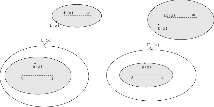
Figure 4: Two complex planes containing the proper contour $\Gamma_{i}(x)$. The shaded regions are forbidden by the conditions in eq. (31).

Moreover, as $t$ encircles $\Gamma_{i}(x)$ once $\omega(x;t)$ encircles $C_{i}$ twice in the positive direction for $i=1$ but in the negative direction for $i=2$. Thus, using also

$$\partial_{t}\omega(x;t)={(t-a(x))(t-b(x))\over t^{2}(t-1)^{2}}$$ (33)

we get (here we also show the intermediate steps discussed above)

$$\oint_{C_{i}}dz\oint_{C_{j}}dw\;\hat{\psi}^{\lambda}_{i}(z)G(\lambda;z,w)\hat{\bar{\psi}}^{\lambda}_{j}(w)=$$

$$=\oint_{C_{i}}dz\oint_{C_{j}}dw\;\hat{\psi}^{\lambda}_{i}(z){1\over z-w}\hat{\bar{\psi}}^{\lambda}_{j}(w)+$$

$$+{1\over 2}\int_{0}^{\lambda}dx\oint_{C_{i}(x)}dz\oint_{C_{j}(x)}dw\hat{\psi}^{\lambda}_{i}(z)\left[-(1+xw)^{-{1\over 2}}(1+xz)^{-{3\over 2}}(w+x)^{{1\over 2}}(z+x)^{-{1\over 2}}+\right.$$

$$\left.+(1+xw)^{{1\over 2}}(1+xz)^{-{1\over 2}}(w+x)^{-{1\over 2}}(z+x)^{-{3\over 2}}\right]\big{(}{z\over w}\big{)}^{\mbox{\scriptsize$\frac{1}{2}$}}\hat{\bar{\psi}}^{\lambda}_{j}(w)=$$ (34)

$$=\oint_{C_{i}}dz\oint_{C_{j}}dw\;\hat{\psi}^{\lambda}_{i}(z){1\over z-w}\hat{\bar{\psi}}^{\lambda}_{j}(w)+$$

$$+{1\over 2}\int_{0}^{\lambda}dx{1\over 4}(-1)^{i+j}\oint_{\Gamma_{i}(x)}dt{(t-a)(t-b)\over t^{2}(t-1)^{2}}\hat{\psi}^{\lambda}_{i}(\omega(x;t))\oint_{\Gamma_{j}(x)}du{(u-a)(u-b)\over u^{2}(u-1)^{2}}\hat{\bar{\psi}}^{\lambda}_{j}(\omega(x;u))$$

$$\left[-{u-b\over u-a}{t^{2}(t-1)^{2}\over(t-a)^{3}(t-b)}+{1\over x^{2}}{u-a\over u-b}{t^{2}(t-1)^{2}\over(t-a)(t-b)^{3}}\right]\left({\omega(x;t)\over\omega(x;u)}\right)^{\mbox{\scriptsize$\frac{1}{2}$}}=$$

$$=\oint_{C_{i}}dz\oint_{C_{j}}dw\;\hat{\psi}^{\lambda}_{i}(z){1\over z-w}\hat{\bar{\psi}}^{\lambda}_{j}(w)+$$

$$-{1\over 2}(-1)^{i+j}\int_{0}^{\lambda}{dx\over x}{ab\over g(x)}\oint_{\Gamma_{i}(x)}{dt\over(t-a)^{2}(t-b)^{2}}\sqrt{\omega(x;t)}\hat{\psi}^{\lambda}_{i}(\omega(x;t))$$

$$\oint_{\Gamma_{j}(x)}{du\over u(u-1)(u-ab)}\sqrt{\omega(x;u)}\hat{\bar{\psi}}^{\lambda}_{j}(\omega(x;u))\left[t^{2}u^{2}-t^{2}u-tu^{2}+ab(u+t)-(ab)^{2}\right]$$ (35)

where one should note that all $a$’s and $b$’s depend on $x$. This will be our final result for the RHS. When we now return to the LHS we will discover that it can be brought to an almost identical form. At the end it will shown that this discrepancy is a total derivative and thus vanishes under the integral.

Returning to the LHS we insert the integral representations (21) and (22) of the $B^{ij}$-matrices:

$$\oint_{C_{i}}dz\oint_{C_{j}}dw\hat{\psi}^{\lambda}_{i}(z)z^{(-1)^{i}r-\mbox{\scriptsize$\frac{1}{2}$}}B^{ij}_{rs}w^{(-1)^{j}s-\mbox{\scriptsize$\frac{1}{2}$}}\hat{\bar{\psi}}^{\lambda}_{j}(w)=$$

$$=(-1)^{i+1}\oint_{C_{i}}dz\oint_{C_{j}}dw\hat{\psi}^{\lambda}_{i}(z)z^{(-1)^{i}r-\mbox{\scriptsize$\frac{1}{2}$}}\left[(1-\delta_{ij})\delta_{rs}+\right.$$

$$\left.+\int_{0}^{\lambda}{dx\over x}(g(x)r\xi_{r}(x)\xi_{s}(x)+(-1)^{i+j}g(x)^{-1}r\eta_{r}(x)\eta_{s}(x))\right]w^{(-1)^{j}s-\mbox{\scriptsize$\frac{1}{2}$}}\hat{\bar{\psi}}^{\lambda}_{j}(w)$$ (36)

To be specific, let us pick the following integral representations for $\xi_{r,s}(x)$ and $\eta_{r,s}(x)$:

$$\xi_{r}(x) = {1\over\sqrt{2}}\oint_{\bar{\Gamma}_{i}(x)}{dt\over t}\omega(x;t)^{-(-1)^{i}r}$$

$$\xi_{s}(x) = {ab-1\over\sqrt{2}}\oint_{\bar{\Gamma}_{j}(x)}{du\over(u-1)(u-ab)}\omega(x;u)^{-(-1)^{j}r}$$

$$\eta_{r}(x) = (-1)^{i+1}{ab\over\sqrt{2}}\oint_{\bar{\Gamma}_{i}(x)}{dt\over t(t-ab)}\omega(x;t)^{-(-1)^{i}r}$$

$$\eta_{s}(x) = (-1)^{j+1}{1\over\sqrt{2}}\oint_{\bar{\Gamma}_{j}(x)}{du\over u-1}\omega(x;u)^{-(-1)^{j}r}$$ (37)

To ensure convergence of the sums over $r,s$ the contours $\bar{\Gamma}_{i}(x)$ are such that $\big{|}z/\omega(x;t)\big{|}^{(-1)^{i}}<1$ for all $z\in C_{i}$ and all $t\in\bar{\Gamma}_{i}(x)$, and analogously with $z\rightarrow w$, $i\rightarrow j$ and $t\rightarrow u$. Here we assume that the contours $C_{i}$ have been collapsed on the branch cuts that they are to encircle in such a way that $|z|>{1\over|\lambda|}$ for all $z\in C_{1}$ and $|z|<|\lambda|$ for all $z\in C_{2}$, and analogously for $z\rightarrow w$. Again using (32), we see that $\bar{\Gamma}_{i}(x)$ have to be drawn as in (5). The sums in the LHS are now well-defined, and we get

$$\oint_{C_{i}}dz\oint_{C_{j}}dw\hat{\psi}^{\lambda}_{i}(z){1\over z-w}\hat{\bar{\psi}}^{\lambda}_{j}(w)\;(1-\delta_{ij})+$$

$$+\mbox{\scriptsize$\frac{1}{2}$}(-1)^{i+j}\oint_{C_{i}}dz\oint_{C_{j}}dw\hat{\psi}^{\lambda}_{i}(z)\left[\int_{0}^{\lambda}{dx\over x}\oint_{\bar{\Gamma}_{i}(x)}dt\sqrt{\omega(x;t)}\oint_{\bar{\Gamma}_{j}(x)}du\sqrt{\omega(x;u)}\right.$$ (38)

$$\left.({\omega(x;t)\over(z-\omega(x;t))^{2}}+\mbox{\scriptsize$\frac{1}{2}$}{1\over z-\omega(x;t)})({g(x)(ab-1)\over t(u-1)(u-ab)}+{g(x)^{-1}(ab)^{2}\over t(t-ab)u(u-ab)}){1\over w-\omega(x;u)}\right]\hat{\bar{\psi}}^{\lambda}_{j}(w)$$

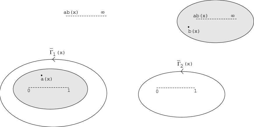
Figure 5: Proper contours $\bar{\Gamma}_{i}(x)$ to be used in the LHS. The shaded regions are forbidden by the conditions for convergence of the sums in eq. (36).

The first term in (38) agrees with the closed result in (35) due to fact that when $i=j$ the first term in (35) vanishes:

$$\oint_{C_{i}}dz\oint_{C_{i}}dw\hat{\psi}^{\lambda}_{i}(z){1\over z-w}\hat{\bar{\psi}}^{\lambda}_{i}(w)=\oint_{C_{i}}dz\big{(}-\oint_{z}\big{)}dw\hat{\psi}^{\lambda}_{i}(z){1\over z-w}\hat{\bar{\psi}}^{\lambda}_{i}(w)=$$

$$=\oint_{C_{i}}dz\hat{\psi}^{\lambda}_{i}(z)\hat{\bar{\psi}}^{\lambda}_{i}(z)=0\;\;,$$ (39)

since in the last expression $C_{i}$ encircles all the singularities of the integrand

In the second term in (38) the contours $C_{i}$ and $C_{j}$ (which are collapsed on the respective branch cuts) and $\bar{\Gamma}_{i}(x)$ and $\bar{\Gamma}_{j}(x)$ are precisely such that change of the order of integration between $\oint_{C_{i}}dz\oint_{C_{j}}dw$ and $\int_{0}^{\lambda}dx\oint_{\bar{\Gamma}_{i}(x)}dt\oint_{\bar{\Gamma}_{j}(x)}du$ is allowed and such that $C_{i}$ and $C_{j}$ can be flipped over to the poles at $z=\omega(x;t)$ and $w=\omega(x;u)$. Using also the identity $(ab-1)g={ab\over g}$ the second term becomes

$$\mbox{\scriptsize$\frac{1}{2}$}(-1)^{i+j}\int_{0}^{\lambda}{dx\over x}{ab\over g(x)}\oint_{\bar{\Gamma}_{i}(x)}dt\sqrt{\omega(x;t)}\oint_{\bar{\Gamma}_{j}(x)}du\sqrt{\omega(x;u)}({\omega(x;t)\over\partial_{t}\omega(x;t)}\partial_{t}\hat{\psi}^{\lambda}_{i}(\omega(x;t))+\mbox{\scriptsize$\frac{1}{2}$}\hat{\psi}^{\lambda}_{i}(\omega(x;t)))$$

$$({1\over t(t-ab)(u-ab)}+{ab\over t(t-ab)u(u-ab)})\hat{\bar{\psi}}^{\lambda}_{j}(\omega(x;u))$$ (40)

We next remove the $t$-derivative on $\hat{\psi}^{\lambda}_{i}$ by integrating by parts. After some simplifications we arrive at

$$-\mbox{\scriptsize$\frac{1}{2}$}(-1)^{i+j}\int_{0}^{\lambda}{dx\over x}{ab\over g(x)}\oint_{\bar{\Gamma}_{i}(x)}{dt\over(t-a)^{2}(t-b)^{2}}\sqrt{\omega(x;t)}\hat{\psi}^{\lambda}_{i}(\omega(x;t))$$ (41)

$$\oint_{\bar{\Gamma}_{j}(x)}{du\over u(u-1)(u-ab)}\sqrt{\omega(x;u)}\hat{\bar{\psi}}^{\lambda}_{j}(\omega(x;u))\left[u(ab-1)(t^{2}-ab)+(u-1)ab(t^{2}-2t+ab)\right]$$

Before comparing (41) to the second term in (35) there is a slight subtlety in (41) which needs to be explained, namely the fact that there is no prescription of how the contours $\bar{\Gamma}_{i}(x)$ are to encircle the poles at $t=a$ and $t=b$. However, the reason for this is simply that these poles have zero residues. These poles stem from the factor $(\partial_{t}\omega(x;t))^{-1}$ which was inserted in (40) in order to compensate for the inner derivative of $\partial_{t}\hat{\psi}^{\lambda}_{i}(\omega(x;t))$. We may write the $t$-integral in (40) as

$$\oint_{\bar{\Gamma}_{i}(x)}dt{f(t)\over(t-a)(t-b)}\partial_{t}\hat{\psi}^{\lambda}_{i}(\omega(x;t))=-\oint_{\bar{\Gamma}_{i}(x)}dt\partial_{t}({f(t)\over(t-a)(t-b)})\hat{\psi}^{\lambda}_{i}(\omega(x;t))=$$

$$=\oint_{\bar{\Gamma}_{i}(x)}dt\big{(}{f(t)\over(t-a)^{2}(t-b)}+{f(t)\over(t-a)(t-b)^{2}}-{f^{\prime}(t)\over(t-a)(t-b)}\big{)}\hat{\psi}^{\lambda}_{i}(\omega(x;t))$$ (42)

where $f$ is analytic at $t=a$ and $t=b$. Thus the residue at e.g. $t=b$ is given by

$${f(b)\over(b-a)^{2}}\hat{\psi}^{\lambda}_{i}(\omega(x;b))+\partial_{t}\left.\big{(}{f(t)\hat{\psi}^{\lambda}_{i}(\omega(x;t))\over t-a}\big{)}\right|_{t=b}-{f^{\prime}(b)\over b-a}\hat{\psi}^{\lambda}_{i}(\omega(x;b))=$$

$$={f(b)\over b-a}{\hat{\psi}^{\prime}_{i}}{}^{\lambda}(\omega(x;b))\partial_{t}\left.\omega(x;t)\right|_{t=b}=0$$

Hence the contours $\bar{\Gamma}_{i}(x)$ in (41) and $\Gamma_{i}(x)$ in (35) are equivalent. The same holds for $\bar{\Gamma}_{j}(x)$ and $\Gamma_{j}(x)$.

Since the contours of integration in the LHS (41) (see fig.(5)) and the RHS (35) (see fig.(4)) are the same, we can now compare the integrand of these two expressions. We then find that they differ only in the square bracket and that this difference, namely

$$\left[t^{2}u^{2}-(t^{2}u+tu^{2})+ab(u+t)-(ab)^{2}\right]-\left[u(ab-1)(t^{2}-ab)+(u-1)ab(t^{2}-2t+ab)\right]=$$

$$=t(t-1)(u-a)(u-b)\;,$$ (43)

gives a vanishing contribution to the integrals over $u$. This can be seen as follows. The contour $\Gamma_{j}(x)$ in (35) (which is now forbidden only in the shaded region in fig. (3) which contains the branch cut in $\hat{\bar{\psi}}^{\lambda}_{j}(\omega(x;u))$) is precisely such that $\hat{\bar{\psi}}^{\lambda}_{j}(\omega(x;u))$ may be expanded in an analytic Taylor series in $\omega(x;u)$ for all $u\in\Gamma_{j}(x)$. Moreover, for positive integers $n$ (in fact we could take $n\in{\bf Z}$):

$$\oint_{\Gamma_{j}(x)}{du\over u(1-u)(u-ab)}\sqrt{\omega(x;u)}\omega(x;u)^{n}(u-a)(u-b)=$$

$$=\oint_{\Gamma_{j}(x)}\partial_{u}\omega(x;u)\omega(x;u)^{n-{1\over 2}}=2\oint_{\infty}dz\;z^{2n}=0$$ (44)

Thus:

$$\oint_{\Gamma_{j}(x)}{du\over u(1-u)(u-ab)}\sqrt{\omega(x;u)}\hat{\bar{\psi}}^{\lambda}_{j}(\omega(x;u))(u-a)(u-b)=0$$ (45)

This completes the proof that the two sides of eq.(12) are equal.

Finally we comment that there is nothing particular about the above choice (37) of integral representations for $\xi_{r,s}$ and $\eta_{r,s}$. Picking another combination of $\xi_{r,s}$ and $\eta_{r,s}$ from (23) and (24) would only modify the $t$ and $x$ dependence in front of the total $u$-derivative that arises when computing the difference between the RHS and the LHS, and would therefore not affect the (unique) propagator $G(\lambda;z,w)$.

There are several directions in which one would like to extend the techniques and results of this paper. We have already mentioned in the introduction the importance of proving the full GGRT (first discussed in the context of the bosonic string in [13, 14]) for twisted fermions. One should investigate to what extent the techniques used in this paper could be modified towards treating more general locally conformal transformations than projective ones. This could turn out to be necessary in order to prove the GGRT for the NSR-string along the lines of the GGRT laid out in [13, 14]. Such considerations should of course incorporate also multi-string multi-loop vertices. However, even if restricting ourselves to projective transformations it does not seem entirely straightforward to apply the techniques that have been developed here also to these more general vertices. This is related to the fact that these methods rely heavily on the simplifications that occur for the matrices $M$ etc when particular choices are made for the projective transformations used to transport the basic dual vertices in a four-string vertex.

We also wish to extend the methods developed here for Ramond four-string vertex to four-string vertices involving other twisted systems. Let us therefore recall the crucial steps of the Ramond case discussed above which must carry over to these other cases. The first step was to find integral representations of the inverse matrices $B^{ij}_{rs}$ and the propagator $G(z,w)$ which factorize in the following sense. For the latter one wants the $z$ and $w$ dependence to factorize (apart from in the simple pole term). This was however an immediate consequence of rewriting it as an integral; see (27). In the former case the factorization refers to the indices $r$ and $s$, and for it to occur it seems necessary to make the particular choice (4) of projective transformations (or any of the closely related ones given in [8]). Namely, this choice implies that $B^{ij}_{rs}$ may be written as in (18) and that $\partial_{\lambda}M(\lambda)$ has rank zero, i.e. $\partial_{\lambda}M(\lambda)\propto Rvv^{T}$ where $v$ is the infinite dimensional vector associated with the massless oscillator modes. The whole four-fermion string vertex is therefore in this sense determined by its massless sector. It is also of crucial importance to have $(1\pm M)^{-1}v$ etc expressed in terms of integral representations of hypergeometric functions. All these features are likely to generalize to other systems; one indication of this is provided by the $\bf{Z}_{3}$ fermionic system treated in [9]. Hence we believe that by means of these methods we can perform the crucial step of “resmoothing” (i.e. deriving closed, geometrical expressions for) arbitrary sewn twisted four-string vertices by means of pure operator sewing methods.

Acknowledgement
We are very grateful to Christian Preitschopf for useful discussions.

References

[1] P. Di Vecchia, ’Multiloop amplitudes in string theories’, talk
at the Workshop
on ’String quantum gravity and physics at the Planck energy scale’, Erice,
June 1992.
[2] E. Corrigan and D. Olive, Nuovo Cimento 11A (1972) 749.
[3] E. Corrigan, Nucl. Phys. B69 (1974) 325.
[4] J.H. Schwarz and C.C. Wu, Phys. Lett. B47 (1973) 453.
[5] E. Corrigan, P. Goddard, R.A. Smith and D. Olive,
Nucl. Phys. B67 (1973) 477.
[12] ”Conformal Invariance and Applications to Statistical
Mechanics”,
Editors C. Itzykson, H. Saleur and J.-B. Zuber,
World Scientific (Singapore 1988).