DAMTP/93-4

20 March 1993

ABSTRACT We introduce the notion of a braided Lie algebra consisting of a finite-dimensional vector space $\cal L$ equipped with a bracket $[\ ,\ ]:\hbox{{$\cal L$}}\mathop{\otimes}\hbox{{$\cal L$}}\to\hbox{{$\cal L$}}$ and a Yang-Baxter operator $\Psi:\hbox{{$\cal L$}}\mathop{\otimes}\hbox{{$\cal L$}}\to\hbox{{$\cal L$}}\mathop{\otimes}\hbox{{$\cal L$}}$ obeying some axioms. We show that such an object has an enveloping braided-bialgebra $U(\hbox{{$\cal L$}})$. We show that every generic $R$-matrix leads to such a braided Lie algebra with $[\ ,\ ]$ given by structure constants $c^{IJ}{}_{K}$ determined from $R$. In this case $U(\hbox{{$\cal L$}})=B(R)$ the braided matrices introduced previously. We also introduce the basic theory of these braided Lie algebras, including the natural right-regular action of a braided-Lie algebra $\cal L$ by braided vector fields, the braided-Killing form and the quadratic Casimir associated to $\cal L$. These constructions recover the relevant notions for usual, colour and super-Lie algebras as special cases. In addition, the standard quantum deformations $U_{q}(g)$ are understood as the enveloping algebras of such underlying braided Lie algebras with $[\ ,\ ]$ on $\hbox{{$\cal L$}}\subset U_{q}(g)$ given by the quantum adjoint action.

1 Introduction

Many authors have sought a description of $U_{q}(g)$ and other quantum groups as generated, in some sense, by a finite-dimensional ‘quantum Lie algebra’ via some kind of enveloping algebra construction (just as $U(g)$ is the universal enveloping algebra of the Lie algebra $g$). Such a notion would be useful since one would only have to work with the finite-dimensional Lie algebra instead of the whole quantum group. It is also important for geometrical applications where we might be interested in quantum vector fields generated by the action not of general elements of the quantum group but by the action of the ‘Lie algebra’ elements.

We are in a situation here where a new mathematical concept is needed: quantum groups $U_{q}(g)$ have various interesting choices of generators but which ones should we look at, and what axioms should they obey? One idea would be to attempt to build this on $g$ itself but with some kind of deformed bracket obeying some kind of new axioms. In [10, Sec. 2] we have initiated a different approach based on the subspace $\{l^{+}Sl^{-}\}\subset U_{q}(g)$ (where $l^{\pm}$ are the FRT generators of $U_{q}(g)$[3]). This subspace is already well-known to be useful for certain kinds of computations and we introduced on it some kind of ‘quantum Lie bracket’ $[\ ,\ ]$ based on the quantum adjoint action and defined by structure constants $c^{IJ}{}_{K}$. This is recalled briefly in Section 2. Our goal in the present paper is to develop this further onto an axiomatic framework for this bracket.

The natural bracket here does not obey of course the Jacobi identities, but rather we find that it obeys naturally some kind of ‘braided-Jacobi identity’. In this notion, which we introduce, the Yang-Baxter operator associated to the action of $U_{q}(g)$ in the adjoint representation plays a central role. Armed with suitable identities we show quite generally that brackets obeying them allow one to generate an entire enveloping algebra.

The problem of defining some kind of braided-Lie algebra has been an open one for some time. The reason is that in a braided setting the Yang-Baxter operator or braided-transposition $\Psi$ does not have square 1. As a result there is no action of the symmetric group and no notion of the Jacobi identity as $0=[\xi,[\eta,\zeta]]+$cyclic. If we do suppose that $\Psi^{2}={\rm id}$ then we are in the symmetric or unbraided situation as studied in [4][21] and elsewhere. In this situation everything goes through just as in the case of usual or super-Lie algebras. Unfortunately, this case is extremely similar to the usual or super case (because $\Psi$ basically has eigenvalues $\pm 1$) so no really new phenomena are obtained. Moreover, it is too restrictive to deal with quantum groups of interest, such as $U_{q}(sl_{2})$.

Our approach to the problem is the following. In a series of papers we have introduced the notion of braided group, see [16][17][12] and others. These are a generalization of quantum groups in which the elements are allowed to have braid statistics. This means that they live in a braided tensor category where the tensor product $\mathop{\otimes}$ is commutative only up to a braided-transposition $\Psi$. Most importantly for us now, we introduced the notion of a braided-cocommutative object of this type. Only such braided-cocommutative objects could be truly expected to be some kind of enveloping algebra. Thus we know the object which we wish to emerge as the enveloping algebra of some kind of braided Lie algebra. By studying the properties of the braided-adjoint action of such objects, we can then deduce the right properties of the braided-Lie algebra itself. These braided groups and the necessary Jacobi-like properties of the braided-adjoint action form the topic of Section 3.

In Section 4 we take the properties of the braided-adjoint action formally as a set of axioms for a braided-Lie algebra. Here we no longer assume that we are given a braided group but rather our main theorem is to show that such braided-Lie algebras indeed generate a braided group or semigroup. By the latter we mean a bialgebra in a braided category without necessarily an antipode. Our main example is developed in Section 5 where we see that the quantum-Lie algebras of Section 2 fit naturally into this axiomatic framework. The construction works for a general $R$-matrix and in this case $U(\hbox{{$\cal L$}})$ recovers the braided matrices $B(R)$ introduced in [17]. There they were introduced as a braided version of a quantum function algebra (like functions on $M_{n}$) but the same braided matrices arise as a braided enveloping bialgebra. It is interesting that only after further quotienting by determinant-type (and other relations) does one recover precisely $U_{q}(g)$ in this way: the braided matrices seem to be a natural covering algebra of these objects and yet have properties like an enveloping algebra. We have already identified the braided matrices covering $U_{q}(sl_{2})$ as a form of Sklyanin algebra at degenerate parameter value[10], which we understand now as $U(\hbox{{$\cal L$}})$ where $\cal L$ is a braided-deformation of $gl_{2}$.

In a different direction we note that the action of such braided-Lie algebras should naturally be some kind of braided-vector field. We demonstrate this in Section 6 where we compute the right-regular action of the generators on $U_{q}(g)$. This was announced in [8] and our goal here is to give the full details. These braided-vector fields are characterised by a matrix-Leibniz rule

$$(ab)\overleftarrow{\partial}{}^{i}{}_{j}=a\cdot\Psi(b\mathop{\otimes}\overleftarrow{\partial}{}^{i}{}_{k})\overleftarrow{\partial}{}^{k}{}_{j}$$

and are the left-invariant (and bicovariant) ‘vector fields’ generated by right-translations of the braided-Lie algebra generators on the braided group. This can be contrasted with other constructions for differential operators on quantum groups. The main difference is that we abandon in our notion of braided-Lie algebras and braided-vector fields a commitment to the usual linear form of the Leibniz rule. This is tied to the linear coproduct $\Delta\xi=\xi\mathop{\otimes}1+1\mathop{\otimes}\xi$. In general for a quantum group there are few such primitive elements. Instead, we work more generally and consider the notions as subordinate to a choice of (braided) coproduct $\Delta$. Aside from the standard linear one, the matrix coproduct then suggests this matrix-notion of Lie algebras and vector fields. For expressions that reduce in the classical limit to usual infinitesimals one need only work with ${\partial}{}^{i}{}_{j}-\delta^{i}{}_{j}$.

Finally, in Section 7 we give another application where the notion of a natural finite-dimensional Lie algebra object is useful, namely to the definition of braided-Killing form. This is provided by the quantum or braided-trace in the adjoint representation of $U(\hbox{{$\cal L$}})$ on $\cal L$. One the generators $u^{i}{}_{j}-\delta^{i}{}_{j}$ one recovers in the classical limit and for standard $R$-matrices the usual Killing form. As an unusual phenomenon we find that the Killing form is made non-degenerate on $gl_{2}=sl_{2}\oplus u(1)$ by the process of braided $q$-deformation. Moreover, our constructions work for any bi-invertible $R$-matrix and we give formulae for the braided-Killing form $g^{IJ}$ in terms of it. In the invertible case it can be used to raise and lower indices (i.e. to identify $\cal L$ and $\hbox{{$\cal L$}}^{*}$) and is Ad-invariant and braided-symmetric in a suitable sense. As an application of the braided-Killing form we compute the corresponding quadratic Casimir

$$C=u^{I}u^{J}g_{IJ}$$

in this invertible case.

2 Quantum Lie Algebras

This section provides some motivation for the constructions of the paper from the point of view of quantum groups. It is perfectly possible to proceed directly to the braided version in the next section and return only for some details needed for the examples in subsequent sections. Throughout the present section some familiarity with quantum groups is assumed. We work over a field $k$ or (with care) a commutative ring (the reader can keep in mind ${{C}}$ or ${{C}}[[\mathchar 1406\relax]]$) and use the usual notations and methods for a quasitriangular Hopf algebra $(H,\Delta,{\epsilon},S,\hbox{{$\cal R$}})$. Here $H$ is a unital algebra, $\Delta:H\to H\mathop{\otimes}H$ is the coproduct, ${\epsilon}:H\to k$ the counit, $S:H\to H$ the antipode and (for a strict quantum group) $\hbox{{$\cal R$}}\in H\mathop{\otimes}H$ is the quasitriangular structure or so-called ‘universal R-matrix’. It obeys the axioms of Drinfeld[2],

$$(\Delta\mathop{\otimes}{\rm id})(\hbox{{$\cal R$}})=\hbox{{$\cal R$}}_{13}\hbox{{$\cal R$}}_{23},\quad({\rm id}\mathop{\otimes}\Delta)(\hbox{{$\cal R$}})=\hbox{{$\cal R$}}_{13}\hbox{{$\cal R$}}_{12},\quad\sum h{}_{(2)}\mathop{\otimes}h{}_{(1)}=\hbox{{$\cal R$}}(\Delta\,h)\hbox{{$\cal R$}}^{-1}.$$ (1)

For an introduction one can see [15]. Here and below we use the Sweedler notation[24] $\Delta h=\sum h{}_{(1)}\mathop{\otimes}h{}_{(2)}$ for the coproduct.

The problem which we consider is the following. It is well-known that the standard quantum-groups $\hbox{{$\cal O$}}_{q}(G)$ of function algebra type can be obtained by an $R$-matrix method as quotients of the quantum matrices $A(R)$ by determinant and other relations[3]. On the other hand, the known treatments of the quantum enveloping algebras to which these are dual, are quite a bit different. There is the approach of Drinfeld and Jimbo in terms of the roots[2][5] and an approach in [3] with twice as many generators $l^{\pm}$ which have to be cut down somehow (usually by means of some imaginative ansatz). These $l^{\pm}$ are roughly speaking the matrix elements of the fundamental and conjugate-fundamental representation of $A(R)$. Here we recall a somewhat different approach based on the quantum Killing form and a single braided-matrix of generators ${\bf u}=(u^{i}{}_{j})$ and developed in [10].

Just as Lie algebras like $sl_{n}$ can be defined both via root systems and via matrices, so we give in this way a matrix approach to the standard quantum enveloping algebras. At the same time a remarkable correspondence principle or self-duality emerges between $\hbox{{$\cal O$}}_{q}(G)$ as a quotient of quantum matrices $A(R)$ and $U_{q}(g)$ as a corresponding quotient of the braided matrices $B(R)$. In the present section we shall try to give a self-contained picture of this using well-known quantum group formulae without too much direct dependence on the theory of braided groups.

Let $R$ in $M_{n}\mathop{\otimes}M_{n}$ be an invertible matrix solution of the quantum Yang-Baxter equations (QYBE) $R_{12}R_{13}R_{23}=R_{23}R_{13}R_{12}$. We recall that $A(R)$ denotes the matrix bialgebra with generators ${\bf t}=(t^{i}{}_{j})$ and relations $R{\bf t}_{1}{\bf t}_{2}={\bf t}_{2}{\bf t}_{1}R$ in the usual compact notation (where the numerical suffices refer to the position in a matrix tensor product). We recall also that $B(R)$ denotes the quadratic algebra with $n^{2}$ generators $\{u^{i}{}_{j}\}$ and $1$, and relations

$$R^{k}{}_{a}{}^{i}{}_{b}u^{b}{}_{c}R^{c}{}_{j}{}^{a}{}_{d}u^{d}{}_{l}=u^{k}{}_{a}R^{a}{}_{b}{}^{i}{}_{c}u^{c}{}_{d}R^{d}{}_{j}{}^{b}{}_{l}\quad{\rm i.e.}\quad R_{21}{\bf u}_{1}R_{12}{\bf u}_{2}={\bf u}_{2}R_{21}{\bf u}_{1}R_{12}.$$ (2)

These relations have been known for some time to be convenient for describing $U_{q}(g)$ but they have been studied formally as a quadratic algebra for the first time in [17]. We will come to the braided aspect[17] in Section 5. For now we just work with $B(R)$ as a quadratic algebra.

Proposition 2.1

The algebra $B(R)$ is dual to $A(R)$ in the following sense. Let $(H,\hbox{{$\cal R$}})$ be a quasitriangular bialgebra which is dually paired by $<\ ,\ >$ with $A(R)$ such that $<{\bf t}_{1}\mathop{\otimes}{\bf t}_{2},\hbox{{$\cal R$}}>=R$. Let

$$l=({\bf t}\mathop{\otimes}{\rm id})(Q),\qquad Q=\hbox{{$\cal R$}}_{21}\hbox{{$\cal R$}}_{12}.$$

Here $l^{i}{}_{j}$ are elements of $H$. Then there is an algebra map $B(R)\to H$ such that $l$ is the image of ${\bf u}$, i.e. $H$ is a realization of $B(R)$.

Proof This is motivated by ideas for $U_{q}(g)$ implicit in the literature, see [20][19]. The new part in our approach however, is to formulate the result at the level of bialgebras. Both $A(R)$ and $B(R)$ are quadratic algebras and no antipode is needed. This approach arises out of the transmutation theory of braided groups that related $A(R)$ to $B(R)$ in [13][12], where we show the useful identity

$$l_{1}R_{12}l_{2}=R_{12}({\bf t}_{1}{\bf t}_{2}\mathop{\otimes}{\rm id})(Q).$$ (3)

To be self-contained we can also give a direct proof of this easily enough as

$$l_{1}R_{12}l_{2} = \sum R_{21}<{\bf t}_{1},Q{{}^{(1)}}><{\bf t}_{1}\mathop{\otimes}{\bf t}_{2},\hbox{{$\cal R$}}><{\bf t}_{2},Q^{\prime}{{}^{(1)}}>Q{{}^{(2)}}Q^{\prime}{{}^{(2)}}$$

$$= \sum<{\bf t}_{1},\hbox{{$\cal R$}}{{}^{(2)}}\hbox{{$\cal R$}}^{\prime}{{}^{(1)}}\hbox{{$\cal R$}}^{\prime\prime\prime\prime}{{}^{(1)}}><{\bf t}_{2},\hbox{{$\cal R$}}^{\prime\prime\prime\prime}{{}^{(2)}}\hbox{{$\cal R$}}^{\prime\prime}{{}^{(2)}}\hbox{{$\cal R$}}^{\prime\prime\prime}{{}^{(1)}}>\hbox{{$\cal R$}}{{}^{(1)}}\hbox{{$\cal R$}}^{\prime}{{}^{(2)}}\hbox{{$\cal R$}}^{\prime\prime}{{}^{(1)}}\hbox{{$\cal R$}}^{\prime\prime\prime}{{}^{(2)}}$$

$$= \sum\hbox{{$\cal R$}}{{}^{(1)}}\hbox{{$\cal R$}}^{\prime\prime}{{}^{(1)}}\hbox{{$\cal R$}}^{\prime}{{}^{(2)}}\hbox{{$\cal R$}}^{\prime\prime\prime}{{}^{(2)}}<{\bf t}_{1},\hbox{{$\cal R$}}{{}^{(2)}}\hbox{{$\cal R$}}^{\prime\prime\prime\prime}{{}^{(1)}}\hbox{{$\cal R$}}^{\prime}{{}^{(1)}}><{\bf t}_{2},\hbox{{$\cal R$}}^{\prime\prime}{{}^{(2)}}\hbox{{$\cal R$}}^{\prime\prime\prime\prime}{{}^{(2)}}\hbox{{$\cal R$}}^{\prime\prime\prime}{{}^{(1)}}>$$

$$= \sum<{\bf t}_{1},\hbox{{$\cal R$}}{{}^{(2)}}{}_{(2)}\hbox{{$\cal R$}}^{\prime\prime\prime\prime}{{}^{(1)}}\hbox{{$\cal R$}}^{\prime}{{}^{(1)}}{}_{(1)}><{\bf t}_{2},\hbox{{$\cal R$}}{{}^{(2)}}{}_{(1)}\hbox{{$\cal R$}}^{\prime\prime\prime\prime}{{}^{(2)}}\hbox{{$\cal R$}}^{\prime}{{}^{(2)}}>\hbox{{$\cal R$}}{{}^{(1)}}\hbox{{$\cal R$}}^{\prime}{{}^{(2)}}$$

$$= \sum<{\bf t}_{1},\hbox{{$\cal R$}}^{\prime\prime\prime\prime}{{}^{(1)}}\hbox{{$\cal R$}}{{}^{(2)}}{}_{(1)}\hbox{{$\cal R$}}^{\prime}{{}^{(1)}}{}_{(1)}><{\bf t}_{2},\hbox{{$\cal R$}}^{\prime\prime\prime\prime}{{}^{(2)}}\hbox{{$\cal R$}}{{}^{(2)}}{}_{(2)}\hbox{{$\cal R$}}^{\prime}{{}^{(2)}}>\hbox{{$\cal R$}}{{}^{(1)}}\hbox{{$\cal R$}}^{\prime}{{}^{(2)}}$$

$$= \sum R_{12}<{\bf t}_{1}{\bf t}_{2},\hbox{{$\cal R$}}{{}^{(2)}}><{\bf t}_{1}{\bf t}_{2},\hbox{{$\cal R$}}^{\prime}{{}^{(1)}}>\hbox{{$\cal R$}}{{}^{(1)}}\hbox{{$\cal R$}}^{\prime}{{}^{(2)}}=R_{12}<{\bf t}_{1}{\bf t}_{2}\mathop{\otimes}{\rm id},Q{{}^{(1)}}>Q{{}^{(2)}}$$

where $\hbox{{$\cal R$}}^{\prime},\hbox{{$\cal R$}}^{\prime\prime}$ etc denote further copies of $\hbox{{$\cal R$}}=\sum\hbox{{$\cal R$}}{{}^{(1)}}\mathop{\otimes}\hbox{{$\cal R$}}{{}^{(2)}}$. For the second equality we recognised the matrix form of the coproduct of the ${\bf t}$ as paired to multiplication in $H$. For the third equality we used the QYBE for $\cal R$. For the fourth and fifth we used the axioms (1) directly. We then wrote the expressions as products in $A(R)$ for the sixth equality and recognized the result.

By permuting the matrix position labels we have equally well $l_{2}R_{21}l_{1}=R_{21}({\bf t}_{2}{\bf t}_{1}\mathop{\otimes}{\rm id})(Q)$. Hence

$$R_{21}l_{1}R_{12}l_{2}=R_{21}R_{12}({\bf t}_{1}{\bf t}_{2}\mathop{\otimes}{\rm id})(Q)=({\bf t}_{1}{\bf t}_{2}\mathop{\otimes}{\rm id})(Q)R_{21}R_{12}=l_{2}R_{21}l_{1}R_{12}$$

using the relations $R{\bf t}_{1}{\bf t}_{2}={\bf t}_{2}{\bf t}_{1}R$ repeatedly.  $\sqcup$$\sqcap$

In this sense then, $B(R)$ is some kind of universal dual algebra to $A(R)$. Just as $A(R)$ has to be cut down by determinant and other relations to obtain an honest Hopf algebra, likewise if $H$ is a Hopf algebra then $B(R)$ is generally a little too big to coincide with $H$: it too has to be cut down by additional relations. Note that in this case where $H$ is a Hopf algebra the elementary identity $\hbox{{$\cal R$}}^{-1}=(S\mathop{\otimes}{\rm id})(\hbox{{$\cal R$}})$ means that $l=l^{+}Sl^{-}$ relating this description of $H$ to the FRT approach in [3]. For the next proposition we concentrate on those standard quantum groups $U_{q}(g)$ which can be put in this FRT form (this includes the deformations of at least the non-exceptional semisimple Lie algebras).

Proposition 2.2

[10] Let $H=U_{q}(g)$ be of FRT form[3] with associated R-matrix $R$ and dually paired with $A(R)$. Then the map $B(R)\to U_{q}(g)$ has kernel given by ‘braided versions’ of the determinant and other relations associated to the Lie group $G$. Hence $U_{q}(g)$ can be identified as $B(R)$ modulo such relations.

Proof The argument in [10] is as a non-trivial corollary of the process of transmutation[13]. This turns the matrix bialgebra $A(R)$ into the braided matrix $B(R)$ and also turns the quotient quantum groups $\hbox{{$\cal O$}}_{q}(G)$ into their braided versions $B_{q}(G)$. This is done in a categorical way (by shifting categories) and transmutes at the same time all constructions such as quantum planes etc on which these objects act. Hence (by these rather general arguments) $B_{q}(G)$ is obtained in a braided version of the way that $\hbox{{$\cal O$}}_{q}(G)$ is obtained. On the other hand, there is also a braided version $BU_{q}(g)$ of $U_{q}(g)$ coinciding as an algebra. Unlike the untransmuted theory the quantum Killing form $Q:B_{q}(G)\to BU_{q}(g)$ is not just a linear map but a map of braided Hopf algebras. For the standard deformations of semisimple Lie algebras it is even an isomorphism. This is the general reason for the correspondence between $\hbox{{$\cal O$}}_{q}(G)$ and $U_{q}(g)$ as quotients of matrices. For a truly self-contained picture one can of course verify the proposition directly by computing in detail the required quotients of $B(R)$. For example, for $U_{q}(sl_{2})$ on must divide $BSL_{q}(2)$ by the braided determinant $ab-q^{2}cb=1$[17].  $\sqcup$$\sqcap$

Note that the additional relations needed to obtain a Hopf algebra like $U_{q}(g)$ in this way from $B(R)$ are such that there exists a braided antipode ${\underline{S}}$ with ${\bf u}{\underline{S}}{\bf u}=1=({\underline{S}}{\bf u}){\bf u}$. This exhibits the remarkable similarity with what is done to obtain a quantum group from $A(R)$, but with one catch: the matrix coproduct ${\underline{\Delta}}{\bf u}={\bf u}\mathop{\otimes}{\bf u}$ does not give a bialgebra in the usual sense (it is not an algebra homomorphism to the usual tensor product). This explains why for a full appreciation of this approach one must understand $B(R)$ correctly as a bialgebra with braid-statistics[17].

Even without such a full picture, Proposition 2.2 does however, provide a quick way of computing $U_{q}(g)$ as well as the corresponding quantum enveloping algebra in a general non-standard but factorizable case. Namely, compute the quadratic algebra $B(R)$ and then impose further determinant-type and other relations. Factorizable means here by definition that the map from the relevant dual of $H$ to $H$ given by evaluation against the first factor of $Q=\hbox{{$\cal R$}}_{21}\hbox{{$\cal R$}}_{12}$ is a surjection[20]. This ensures in Proposition 2.1 that for such $H$ the $l$ are generators. Note also that the existence of a quasitriangular Hopf algebra dually paired to $A(R)$ is not possible for all $R$. A necessary condition is thet $R$ has a second inverse $\widetilde{R}=<{\bf t}_{1}\mathop{\otimes}{\bf t}_{2},({\rm id}\mathop{\otimes}S)\hbox{{$\cal R$}}>=((R^{t_{2}})^{-1})^{t_{2}}$ (where $t_{2}$ is transposition in the second matrix factor).

For the moment we can just note then that $U_{q}(g)$ and in general any quasitriangular Hopf algebra dual to $A(R)$ has a subspace

$$\hbox{{$\cal L$}}={\rm span}<l^{i}{}_{j}>\subset H$$ (4)

Proposition 2.3

[10]

i) In the factorizable case[20], the subspace $\hbox{{$\cal L$}}={\rm span}<l^{i}{}_{j}>$ and $1$ generate all of $H$. ii) The subspace $\cal L$ is stable under the quantum adjoint action of $H$ on itself.

iii) The quantum adjoint action as a map $[\ ,\ ]:\hbox{{$\cal L$}}\mathop{\otimes}\hbox{{$\cal L$}}\to\hbox{{$\cal L$}}$ looks explicitly like

$$[l^{I},l^{J}]=c^{IJ}{}_{K}l^{K},\quad c^{IJ}{}_{K}=\widetilde{R}{}^{a}{}_{i_{1}}{}^{j_{0}}{}_{b}R^{-1}{}^{b}{}_{k_{0}}{}^{i_{0}}{}_{c}R^{k_{1}}{}_{n}{}^{c}{}_{m}R^{m}{}_{a}{}^{n}{}_{j_{1}}$$

where $l^{I}=l^{i_{0}}{}_{i_{1}}$ and $I=(i_{0},i_{1})$ is a multi-index notation (running from $(1,1),\cdots,(n,n)$).

Proof Again, the proof in [10] is based on the theory of transmutation in [13][12]. The linear space of $B(R)$ can be identified with that of $A(R)$ with the generators ${\bf u}={\bf t}$ identified (but not their products as we have seen above). Then (ii) is automatic because ${\bf t}$ transforms to a linear combination under the quantum coadjoint action, hence so does ${\bf u}$ under the quantum adjoint action. To be self-contained we can also give a direct proof using more familiar methods as follows.

(i) In the present setting this is (as we have mentioned) more or less by the definition of factorizable. In our usage this notion is subordinate to the choice of a bialgebra or Hopf algebra dually paired with $H$ in the sense of [15]. Here the choice is $A(R)$ or its quotients such as $\hbox{{$\cal O$}}_{q}(G)$.

(ii) We use the form $l=l^{+}Sl^{-}$ valid in the Hopf algebra case and let ${\triangleright}={\rm Ad}$ denote the quantum adjoint action of $H$ on itself given by $h{\triangleright}b=\sum h{}_{(1)}bSh{}_{(2)}$. We show that[14]

$$l^{+}_{2}{\triangleright}l_{1}=R^{-1}l_{1}R,\qquad l^{-}_{1}{\triangleright}l_{2}=Rl_{2}R^{-1}$$ (5)

using the definition of ${\rm Ad}$, elementary properties of the antipode and the fact that $l^{\pm}$ obey the relations $R^{-1}l^{\pm}_{1}l^{\pm}_{2}=l^{\pm}_{2}l^{\pm}_{1}R^{-1}$ and $R^{-1}l^{-}_{1}l^{+}_{2}=l^{+}_{2}l^{-}_{1}R^{-1}$ as in [3] (These relations are not tied to the standard $U_{q}(g)$ as in [3] if one uses the general formulation as in [15][14]). Thus

$$l^{+}_{2}{\triangleright}(l^{+}_{1}Sl^{-}_{1}) =l^{+}_{2}l^{+}_{1}Sl^{-}_{1}Sl^{+}_{2}=l^{+}_{2}l^{+}_{1}S(l^{+}_{2}l^{-}_{1})=l^{+}_{2}l^{+}_{1}R^{-1}S(Rl^{+}_{2}l^{-}_{1})$$

$$=R^{-1}l^{+}_{1}l^{+}_{2}S(l^{-}_{1}l^{+}_{2})R=R^{-1}l^{+}_{1}(l^{+}_{2}Sl^{+}_{2})Sl^{-}_{1}R=R^{-1}l^{+}_{1}Sl^{-}_{1}R$$

$$l^{-}_{1}{\triangleright}(l^{+}_{2}Sl^{-}_{2}) =l^{-}_{1}l^{+}_{2}Sl^{-}_{2}Sl^{-}_{1}=l^{-}_{1}l^{+}_{2}S(l^{-}_{1}l^{-}_{2})=l^{-}_{1}l^{+}_{2}RS(R^{-1}l^{-}_{1}l^{-}_{2})$$

$$=Rl^{+}_{2}l^{-}_{1}S(l^{-}_{2}l^{-}_{1})R^{-1}=Rl^{+}_{2}(l^{-}_{1}Sl^{-}_{1})Sl^{-}_{2}R^{-1}=Rl^{+}_{2}Sl^{-}_{2}R^{-1}.$$

(iii) We can also deduce from this the action of $Sl^{\pm}$ from $l^{+}Sl^{+}={\rm id}=(Sl^{+})l^{+}$ etc (the identity matrix times the action of the identity). In particular,

$$({{\scriptstyle S}}l^{-}{}^{i}{}_{j}){\triangleright}l^{k}{}_{l}=\widetilde{R}{}^{a}{}_{j}{}^{k}{}_{m}l^{m}{}_{n}R^{i}{}_{a}{}^{n}{}_{l}.$$ (6)

where $\widetilde{R}$ obeys $\widetilde{R}^{i}{}_{a}{}^{b}{}_{l}R^{a}{}_{j}{}^{k}{}_{b}=\delta^{i}{}_{j}\delta^{k}{}_{l}=R^{i}{}_{a}{}^{b}{}_{l}\widetilde{R}^{a}{}_{j}{}^{k}{}_{b}.$ Combining this with (5) we can compute $l^{i_{0}}{}_{i_{1}}{\triangleright}l^{j_{0}}{}_{j_{1}}=l^{+}{}^{i_{0}}{}_{a}{\triangleright}((Sl^{-}{}^{a}{}_{i_{1}}){\triangleright}l^{j_{0}}{}_{j_{1}}$ to find the result stated.  $\sqcup$$\sqcap$

Thus $\cal L$ is some kind of ‘quantum Lie algebra’ for $H$ because it is a finite-dimensional subspace that generates $H$ and at the same time is closed under the quantum adjoint action, which provides a kind of ‘quantum Lie bracket’ $[\xi,\eta]=\xi{\triangleright}\eta$. We have introduced this point of view in [10] and pointed out that this bracket obeys a number of Lie-algebra-like identities inherited from the standard properties of the quantum adjoint action, such as

(L0) $\qquad[\xi,\eta]\in\hbox{{$\cal L$}}\qquad{\rm for}\qquad\xi,\eta\in\hbox{{$\cal L$}}$

(L1) $\qquad[\xi,[\eta,\zeta]]=\sum[[\xi{}_{(1)},\eta],[\xi{}_{(2)},\zeta]]$

(L$1^{\prime}$) $\qquad[[\xi,\eta],\zeta]=\sum[\xi{}_{(1)},[\eta,[{{\scriptstyle S}}\xi{}_{(2)},\zeta]]]$

The second of these is just the statement that ${\rm Ad}$ is a covariant action of the Hopf algebra on itself, while the third follows from the definition of ${\rm Ad}$. We see here two problems with this approach. Firstly, these properties (L1) and (L$1^{\prime}$) cannot be taken as abstract properties of some kind of Lie algebra structure on $\cal L$ because they involve the coproduct and this does not in general act on $\cal L$ in a simple way (its just gives some subspace of $H\mathop{\otimes}H$). Secondly, they hold for any Hopf algebra and so do not express the fact that quantum groups such as $U_{q}(g)$ are close to being cocommutative. The usual Lie bracket has properties inherited from the fact that $U(g)$ is cocommutative, and our quantum Lie algebra, to be convincing, should deform some of these. For later reference,

Proposition 2.4

If $H$ is a cocommutative Hopf algebra then the usual Hopf algebra adjoint action $[\ ,\ ]={\rm Ad}$ obeys in addition to the identities above, the identities

(L2) $\qquad\sum\xi{}_{(2)}\mathop{\otimes}[\xi{}_{(1)},\eta]=\sum\xi{}_{(1)}\mathop{\otimes}[\xi{}_{(2)},\eta]$

(L3) $\qquad\sum[\xi,\eta]{}_{(1)}\mathop{\otimes}[\xi,\eta]{}_{(2)}=\sum[\xi{}_{(1)},\eta{}_{(1)}]\mathop{\otimes}[\xi{}_{(2)},\eta{}_{(2)}]$

for all $\xi,\eta$ in $H$.

Proof (L2) needs no comment except to say that we have written the cocommutativity in this way because later we shall adopt something like this without assuming that the Hopf algebra is completely cocommutative. This weak notion of cocommutativity (as relative to something on which the Hopf algebra acts) is useful in other contexts also. For (L3) we have $\Delta[\xi,\eta]=\sum\xi{}_{(1)}{}_{(1)}\eta{}_{(1)}S\xi{}_{(2)}{}_{(2)}\mathop{\otimes}\xi{}_{(2)}{}_{(1)}\eta{}_{(2)}S\xi{}_{(2)}{}_{(1)}$ using that $S$ is an anticoalgebra map. In the cocommutative case the numbering of the suffices does not matter so we have at once the right hand side of (L3). For the record we give here also the proof of (L1). This holds for any Hopf algebra and reads

$$\sum[[\xi{}_{(1)},\eta],[\xi{}_{(2)},\zeta]]{\!\!\!\!\!\!}{\!\!\!\!\!\!} =\sum(\xi{}_{(1)}{}_{(1)}\eta S\xi{}_{(1)}{}_{(2)}){}_{(1)}(\xi{}_{(2)}{}_{(1)}\zeta S\xi{}_{(2)}{}_{(2)})S(\xi{}_{(1)}{}_{(1)}\eta S\xi{}_{(1)}{}_{(2)}){}_{(2)}$$

$$=\sum\xi{}_{(1)}\eta{}_{(1)}(S\xi_{(4)})\xi_{(5)}\zeta(S\xi_{(6)})(S^{2}\xi{}_{(3)})(S\eta{}_{(2)})(S\xi{}_{(2)})$$

$$=\sum\xi{}_{(1)}\eta{}_{(1)}\zeta(S\xi_{(4)})(S^{2}\xi{}_{(3)})(S\eta{}_{(2)})(S\xi{}_{(2)})=\xi{}_{(1)}\eta{}_{(1)}\zeta(S\eta{}_{(2)})(S\xi{}_{(2)})=[\xi,[\eta,\zeta]]$$

expanding out the definitions, the properties of the antipode and the Sweedler notation [24] to renumber the suffices to base 10 (keeping the order). The third and fourth equalities then successively collapse using the axioms of an antipode.  $\sqcup$$\sqcap$

Another aspect of our matrix approach, which is not a problem but a convention is that our chosen finite-dimensional subspace $\cal L$ is a mixture of ‘group-like’ elements with coproduct $\Delta\xi\sim\xi\mathop{\otimes}\xi$ and more usual Lie-algebra-like elements where $\Delta\xi\sim\xi\mathop{\otimes}1+1\mathop{\otimes}\xi$ (with a suitable deformation). The latter are how off-diagonal elements of $l^{i}{}_{j}$ tend to behave, while the former are how diagonal elements tend to behave. Another good convention is to take as ‘quantum Lie algebra’ the subspace

$$\hbox{{$\cal X$}}={\rm span}<\chi^{i}{}_{j}>\subset H,\quad\chi^{i}{}_{j}=l^{i}{}_{j}-\delta^{i}{}_{j}$$ (7)

This is a matter of taste and is entirely equivalent. The subspace is also closed under $[\ ,\ ]={\rm Ad}$ which now has structure constants

$$[\chi^{I},\chi^{J}]=[l^{I},l^{J}]+\delta^{I}\delta^{J}-\delta^{I}\delta^{J}-\delta^{I}l^{J}=(c^{IJ}{}_{K}-\delta^{I}\delta^{J}{}_{K})\chi^{K}$$ (8)

using the elementary properties of the quantum adjoint action (notably $l^{I}{\triangleright}1={\epsilon}(l^{I})=\delta^{I}$). Here $\delta^{I}=\delta^{i_{0}}_{i_{1}}$ and $\delta^{J}{}_{K}$ are Kronecker delta-functions. The last equality uses that

$$c^{I}{}^{J}{}_{K}\delta^{K}=\delta^{I}\delta^{J}$$ (9)

which follows at once from the expression for $c$ in the proposition. These $\chi^{I}$ equally generate $H$ along with $1$ and have a better-behaved semi-classical limit in the standard cases. This aspect of our approach has been stressed in [22]. It is also quite natural from the point of view of bicovariant differential calculus as explained in [23]. We note also that some combinations of the basis elements of $\cal L$ or $\cal X$ can have trivial quantum Lie bracket and have to be decoupled if we want to have the minimum number of generators.

Finally, to complete the picture of $B(R)$ as a some kind of dual of $A(R)$ we have an elementary lemma which we will need later in Section 6.

Lemma 2.5

The generators of $A(R)$ define matrix elements of the representation $\rho$ of $B(R)$ given by

$$\rho_{2}({\bf u}_{1})=<{\bf u}_{1},{\bf t}_{2}>=Q_{12},\quad Q=R_{21}R_{12}$$

Proof We have to show that this extends consistently to all of $B(R)$ as an algebra representation,

$$\rho_{3}(R_{21}{\bf u}_{1}R_{12}{\bf u}_{2}) = R_{21}\rho_{3}({\bf u}_{1})R_{12}\rho_{3}({\bf u}_{2})$$

$$= R_{21}Q_{13}R_{12}Q_{23}=Q_{23}R_{21}Q_{13}R_{12}$$

$$= \rho_{3}({\bf u}_{2})R_{21}\rho_{3}({\bf u}_{1})R_{12}=\rho_{3}({\bf u}_{2}R_{21}{\bf u}_{1}R_{12}).$$

The middle equality follows from repeated use of the QYBE. Thus the extension is consistent with the algebra relations of $B(R)$.  $\sqcup$$\sqcap$

One can also see over ${{C}}$ that if $R$ obeys a certain reality condition then $B(R)$ is a $*$-algebra with $u^{i}{}_{j}{}^{*}=u^{j}{}_{i}$. We call this the hermitian real form of the braided matrices $B(R)$. At the level of the standard $U_{q}(g)$ with real $q$ the corresponding $l^{i}{}_{j}{}^{*}=l^{j}{}_{j}$ recovers the standard compact real form of the these Hopf algebras. These remarks confirm that the braided-matrix approach to $U_{q}(g)$ is quite natural.

3 Properties of the Braided-Adjoint Action

In this section we recall some basic facts about Hopf algebras in braided categories (braided Hopf-algebras) and their braided adjoint action. It is these categorical constructions that lead to the notion of braided-Lie algebras in the next section. The idea is that we know what is a braided group[9] (or in physical terms a group-like object with braid statistics[16]) and we just have to infinitesimalize this notion.

One of the novel aspects of braided groups is that results fully analogous to those familiar in algebra or group theory are proven now using braid and knot diagrams. This is because we work in a braided or quasitensor category. This means $(\hbox{{$\cal C$}},\mathop{\otimes},{\underline{1}},\Phi,\Psi)$ where $\cal C$ is a category (a collection of objects and allowed morphisms or maps between them), $\mathop{\otimes}$ is a tensor product between two objects, with ${\underline{1}}$ a unit object for the tensor product. The isomorphisms $\Phi_{V,W,Z}:V\mathop{\otimes}(W\mathop{\otimes}Z)\to(V\mathop{\otimes}W)\mathop{\otimes}Z$ express associativity and say that we can forgot about brackets (all tensor products can be put into a canonical form in a consistent way). Finally, there is a braided-transposition or quasisymmetry $\Psi_{V,W}:V\mathop{\otimes}W\to W\mathop{\otimes}V$ saying that the tensor product is commutative up to this isomorphism. The difference between this setting and the standard one for symmetric monoidal categories[7] is that we do not suppose that $\Psi_{W,V}\circ\Psi_{V,W}={\rm id}$. Put another way, we distinguish carefully between $\Psi_{V,W}$ and $(\Psi_{W,V})^{-1}$ which are both morphisms $V\mathop{\otimes}W\to W\mathop{\otimes}V$ for any two objects. To avoid confusion a good notation here is to write the morphisms not in the usual way as single arrows, but downward as braid crossings,

These braided-transpositions do however obey other obvious properties of usual transposition such as $\Psi_{V\mathop{\otimes}W,Z}=\Psi_{V,Z}\circ\Psi_{W,Z}$ and similarly for $\Psi_{V,W\mathop{\otimes}Z}$. These ensure that different sequences of braided transpositions that connect two composite objects coincide if the corresponding braids in the notation above coincide. Also, these isomorphisms are functorial in that they are compatible with any morphisms between objects. If we write any morphisms also pointing downwards as notes with input lines and output lines, then the functoriality says that we can pull such nodes through braid crossings much as beads on a string.

Figure 1: Axioms of a Braided Hopf Algebra

This describes the diagrammatic notation that we shall use. For a formal treatment of braided categories see [6] and for on introduction to our methods see [8, Sec. 3]. In this notation, the axioms of a Hopf algebra in a braided category are recalled in Figure 1. They are like a usual Hopf algebra $B$ except that the product, coproduct $\Delta$, antipode $S$, unit $\eta$ and counit ${\epsilon}$ are all morphisms in the braided category. In the diagrammatic notation we write the unit object as the empty set. The first axiom shown (the bialgebra axiom) is the most important: it says that the braided coproduct $B\to B{\underline{\mathop{\otimes}}}B$ is an algebra homomorphism where $B{\underline{\mathop{\otimes}}}B$ is the braided tensor product algebra structure on $B\mathop{\otimes}B$. This is like a super-tensor product and involves transposition by $\Psi$. The two factors $B$ in $B{\underline{\mathop{\otimes}}}B$ do not commute but instead enjoy braid statistics given by $\Psi$.

The reader can keep in mind the trivially braided group (the ordinary group Hopf algebra) $B={{C}}G$ with $\Delta g=g\mathop{\otimes}g$ and $Sg=g^{-1}$. The antipode axiom says that if we split $g$ into $g,g$, apply $S$ to one factor and then multiply up, we get something trivial. The diagrams on the right in Figure 1 just say this abstractly as morphisms.

It is remarkable that such objects defined in this way really behave like usual groups or quantum groups. For example, the usual adjoint action of a group on itself consists in taking $g,a$, splitting $g$ to give $g,g,a$, applying $S$ to give $g,g^{-1},a$, transposing $g^{-1}$ past the $a$, and then multiplying up. When written as diagrams or morphisms in our braided category, this is the braided adjoint action. It is shown in the box in Figure 2.

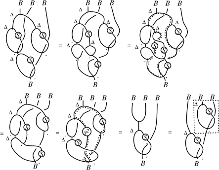
Figure 2: Proof that the braided adjoint action obeys the braided Jacobi identity

Figure 2 itself is the diagrammatic proof of the main result of this section. It shows that applying the braided adjoint action twice as on the right in Figure 2, is the same as the left hand expression. This consists in applying the tensor product braided adjoint action of $B$ on $B\mathop{\otimes}B$ and then applying the adjoint action again to the result (all together three applications of the braided adjoint action on the left in Figure 2). We call this the braided-Jacobi identity. The proof reads as follows. Starting on the left, use the bialgebra axiom that $\Delta$ is an algebra homomorphism to expand the expression on the left. For the second equality we use the fact that $S$ is a braided anti-coalgebra map $\Delta\circ S=(S\mathop{\otimes}S)\Psi\circ\Delta$[18]. We then identify (the dotted line) a closed loop which will after reorganization or the branches using associativity and coassociativity cancel according to the antipode axioms in Figure 1. We make this cancellation for the third equality. We then use that $S$ is a braided anti-algebra map for the fourth equality and identify another loop. This cancels in a similar way to the antipode loop giving the fifth equality. The final equality is the easier fact already proven in [12] that the braided adjoint action is indeed an action. We summarise this along with some other known properties.

Proposition 3.1

Let $B$ be a Hopf algebra in a braided or quasitensor category and let ${\rm Ad}=\cdot^{2}\circ({\rm id}\mathop{\otimes}\Psi_{B,B})({\rm id}\mathop{\otimes}S\mathop{\otimes}{\rm id})(\Delta\mathop{\otimes}{\rm id})$ denote the braided adjoint action as above. It is (a) an action of $B$ on itself and (b) respects its own product (a braided module algebra) as in Figure 3. Further (c) it obeys the braided Jacobi identity. Finally, if $B$ is cocommutative with respect to ${\rm Ad}$ in the sense of [16] (as shown) then (d) holds.

Figure 3: Summary of Properties of the Braided Adjoint Action (a) an action (b) a module-algebra under the action (c) the braided Jacobi identity (d) compatibility with the coproduct implied by the assumption of braided-cocommutativity with respect to ${\rm Ad}$

Proof We have spelled out the proofs of (a),(b) and (d) in [12] in a dual form with comodules and coactions (for the braided adjoint coaction). We ask the reader to turn the diagrammatic proofs for these in [12] up-side down (a 180 rotation) and read them again. They read exactly as the required proof for the ${\rm Ad}$ action. This is part of the self-duality of the axioms of a Hopf algebra. For the new part (c) we have given the proof above.  $\sqcup$$\sqcap$

Note that for a usual non-cocommutative Hopf algebra the quantum adjoint action does not respect the coproduct in the sense of (c) above. One needs a cocommutativity condition. The idea in [16] was not to try to define this intrinsically (the naive notion does not work well) but in a week form as cocommutative with respect to a module. This is the form that we have used: we suppose that $B$ is cocommutative in this weak sense. This corresponds to directly assuming (L2) in Proposition 2.4. This is then enough to derive (d) which corresponds to (L3) in that proposition.

To this extent then, the kind of Hopf algebras in braided categories that we consider are truly like groups or enveloping algebras in the sense that they are supposed braided-cocommutative at least with respect to their own braided adjoint action. This completes our review of the braided adjoint action and the derivation of the identities that we will need in the next section. We will take them as the defining properties of a braided-Lie algebra.

4 Braided-Lie Algebras and their Enveloping Algebras

We have seen that if we do have a braided group as in the last section then the braided-Adjoint action obeys some Lie-algebra like identities as in the second line in Figure 3. If the braided group has some generating subobject which is closed under ${\rm Ad}$ then these identities hold for it also. Motivated by this, we are going to adopt these as abstract axioms for a braided Lie algebra and prove a theorem in the converse direction. Thus every such braided Lie algebra will have (at least in a category with direct sums) an enveloping braided-bialgebra returning us to something like the the kind of braided group we might have began with. One surprise will be that the enveloping algebra here seems more naturally to be a bialgebra (in a braided sense) rather than a Hopf algebra with antipode. Of course one can add further conditions to force a braided-antipode but they do not appear to be very natural from the point of view of the underlying braided Lie algebra.

Definition 4.1

A braided Lie algebra is $(\hbox{{$\cal L$}},\Delta,{\epsilon},[\ ,\ ])$ where $\cal L$ is an object in a braided or quasitensor category, $\Delta:\hbox{{$\cal L$}}\to\hbox{{$\cal L$}}\mathop{\otimes}\hbox{{$\cal L$}}$ and ${\epsilon}:\hbox{{$\cal L$}}\to{\underline{1}}$ are morphisms forming a coalgebra in the category, and $[\ ,\ ]:\hbox{{$\cal L$}}\mathop{\otimes}\hbox{{$\cal L$}}\to\hbox{{$\cal L$}}$ is a morphism obeying the conditions (L1),(L2),(L3) in Figure 4.

Figure 4: Axioms of a Braided Lie Algebra (a) Braided-Jacobi identity axiom (b) Cocommutativity axiom (c) Coalgebra compatibility axiom

The idea of introducing a coalgebra here is one of the novel aspects of the approach. In the usual definition of a Lie algebra a coalgebra structure $\Delta\xi=\xi\mathop{\otimes}1+1\mathop{\otimes}\xi$ and ${\epsilon}\xi=0$ is implicit. We do not want to be tied to a specific form such as this and hence bring the implicit $\Delta$ to the foreground as part of the axiomatic structure. The only requirements of a coalgebra are

$$(\Delta\mathop{\otimes}{\rm id})\circ\Delta=({\rm id}\mathop{\otimes}\Delta)\circ\Delta,\quad({\epsilon}\mathop{\otimes}{\rm id})\circ\Delta={\rm id}=({\rm id}\mathop{\otimes}{\epsilon})\circ\Delta$$ (10)

as usual.

There is no bialgebra axiom here because after all $\cal L$ is not being required to have an associative product. It is typically some finite-dimensional vector space. Instead axiom (L1) says that $\cal L$ is being equipped with some kind of Lie bracket $[\ ,\ ]$. This braided-Jacobi identity is a form of associativity. If one imagines momentarily the usual linear form for $\Delta$ then the left hand side of (L1) has two terms then we have something like the usual Jacobi identity as discussed in Section 2. We of course do not suppose this (we do not even suppose that $\cal L$ has an element that can be called $1$). We do however suppose that $\Delta$ is braided-cocommutative with respect to this Lie bracket $[\ ,\ ]$ in the sense of (L2) and that $\Delta$ respects it in the sense of (L3). This (L3) is a Lie form of the bialgebra condition in Figure 1.

Proposition 4.2

Let $(\hbox{{$\cal L$}},\Delta,{\epsilon},[\ ,\ ])$ be a braided Lie algebra in an Abelian braided tensor category (we suppose that we have direct sums with the usual properties). Then there is a braided bialgebra $U(\hbox{{$\cal L$}})$ in the sense of Section 3, generated by $1$ and $\cal L$ with relations as shown in Figure 5. We call it the universal enveloping algebra of the braided Lie algebra.

Figure 5: Defining relations of the braided enveloping algebra $U(\hbox{{$\cal L$}})$

Proof Formally $U(\hbox{{$\cal L$}})$ is the free tensor algebra generated by $\cal L$ modulo these relations with coproduct given by $\Delta$ extended to products as a braided bialgebra. We have to show that this extension is compatible with the relations of $U(\hbox{{$\cal L$}})$. This is shown in Figure 6. The first equality is the definition of how $\Delta$ extends to products. The second assumes the relations in $U(\hbox{{$\cal L$}})$. The third is coassociativity and functoriality. The fourth uses the cocommutativity axiom (L2) applied in reverse. The fifth uses functoriality and coassociativity again to reorganise. The sixth equality is (L3). The result the coincides with the extension of $\Delta$ to products when the relations of $U(\hbox{{$\cal L$}})$ are used first. The proof to higher order proceeds similarly by induction. The proof that ${\epsilon}$ also extends to a counit on $U(\hbox{{$\cal L$}})$ is equally straightforward.  $\sqcup$$\sqcap$

Figure 6: Proof that $\Delta$ extends to $U(\hbox{{$\cal L$}})$ as a braided bialgebra

The motivation here is as follows. In any Hopf algebra one has the identity $\sum[\xi{}_{(1)},\eta]\xi{}_{(2)}=\sum\xi{}_{(1)}{}_{(1)}\eta(S\xi{}_{(1)}{}_{(2)})\xi{}_{(2)}=\xi\eta$. For example for the usual $U(g)$ with linear coproduct this is $[\xi,\eta]+\eta\xi=\xi\eta$ as expected. We have a similar definition but without any specific form of coalgebra, and of course in the braided setting. We conclude with some general properties of these braided enveloping algebras $U(\hbox{{$\cal L$}})$. Following the usual ideas about Lie algebras representations we have

Definition 4.3

A representation of a braided Lie algebra $(\hbox{{$\cal L$}},\Delta,{\epsilon},[\ ,\ ])$ is an object $V$ and morphism $\alpha:\hbox{{$\cal L$}}\mathop{\otimes}V\to V$ such that the polarised form of the braided-Jacobi identity (L1) holds. This is shown in Figure 7 (a). We say that $\cal L$ is cocommutative with respect to $V$ if the polarised form of the cocommutativity axiom (L2) holds. This is shown in part (b).

Figure 7: Definition (a) of representation of a braided Lie algebra and (b) cocommutativity with respect to it

One can tensor product representations of a braided Lie algebra (using the coproduct $\Delta$) just as for braided Hopf algebras. The class $\hbox{{$\cal O$}}(\hbox{{$\cal L$}})$ of representations with respect to which $\cal L$ is cocommutative is also closed under tensor product and braided with braiding given by $\Psi$. The facts are just as for the representation theory of braided Hopf algebra or bialgebra[18]. The diagrammatic proofs are similar. Alternatively, these facts follow from the following proposition that connects representations of $\cal L$ to those of $U(\hbox{{$\cal L$}})$ for which the bialgebra theory already developed applies.

Proposition 4.4

Every representation $(\alpha,V)$ of a braided Lie algebra $\cal L$ extends a representation of $U(\hbox{{$\cal L$}})$ on $V$. If $\cal L$ is cocommutative with respect to $V$ in the sense of (L2) then $U(\hbox{{$\cal L$}})$ is cocommutative with respect to $V$ in a similar sense (as in [16]).

Figure 8: Proof that (a) a representation on $V$ extends from $\cal L$ to $U(\hbox{{$\cal L$}})$ and (b) cocommutativity also extends

Proof This is shown in Figure 8. Part (a) verifies that the relations of $U(\hbox{{$\cal L$}})$ are represented correctly. We define the action of $U(\hbox{{$\cal L$}})$ by the repeated application of the Lie algebra action as shown. The representation axiom in Definition 4.3 ensures that this coincides with the action of $U(\hbox{{$\cal L$}})$ if its relations are used first. Part (b) verifies that the resulting action is cocommutative if the representation is cocommutative. We show it on elements of $U(\hbox{{$\cal L$}})$ with are products of $\cal L$. The proof proceeds similarly by induction to all orders. The first equality uses Proposition 4.2 that $U(\hbox{{$\cal L$}})$ is a bialgebra. The second equality is functoriality to pull one of the products into the position shown, and that $\alpha$ is a representation for the other product. The third equality is functoriality again to pull one of the $\alpha$’s up to the right. We then use the cocommutativity assumption for the fourth equality, and then again for the fifth. We then use that $\alpha$ is an action and the bialgebra property of $U(\hbox{{$\cal L$}})$ in reverse.  $\sqcup$$\sqcap$

An important example is of course provided by $[\ ,\ ]$ itself. It was the model for the definitions and is clearly a representation and $\cal L$ is cocommutative with respect to it. We call it the adjoint representation of $\cal L$ on itself. By the last proposition then, it extends to a representation (also denoted $[\ ,\ ]$) of $U(\hbox{{$\cal L$}})$ on $\cal L$ with respect to which $U(\hbox{{$\cal L$}})$ is cocommutative.

Lemma 4.5

The adjoint representation $[\ ,\ ]$ of $U(\hbox{{$\cal L$}})$ on $\cal L$ defined via Proposition 4.4 obeys an extended form of the braided-Jacobi identity (L1) and the coalgebra compatibility property (L3) in which the left-most input $\cal L$ in Figure 4 is extended to $U(\hbox{{$\cal L$}})$.

Figure 9: Proof that (a) property (L1) and (b) property (L3) extend to representation $[\ ,\ ]$ of $U(\hbox{{$\cal L$}})$ on $\cal L$

Proof This is shown in Figure 9. Part (a) verifies the extended braided-Jacobi identity on elements of $U(\hbox{{$\cal L$}})$ which are products of $\cal L$. The first equality uses that $U(\hbox{{$\cal L$}})$ is a braided bialgebra from Proposition 4.2. The second that $[\ ,\ ]$ is a representation of $U(\hbox{{$\cal L$}})$ as obtained from Proposition 4.4. We then successively use the braided Jacobi identity axiom (L1) twice. The final equality uses again that $[\ ,\ ]$ is an action. Exactly the same proof holds with the elements in $U(\hbox{{$\cal L$}})$ is a higher order composite element, provided only that the result has been proved already at lower orders so that we can use it for the third and fourth equalities. Hence the result is proven to all orders by induction. Part (b) is proved in a similar way. We verify (L3) extended to products in its first input. The first equality is that $[\ ,\ ]$ is a representation. The second and third successively use (L3). The fourth then uses that $[\ ,\ ]$ is an action and the fifth that $U(\hbox{{$\cal L$}})$ is a bialgebra. The proof extends to all orders by induction.  $\sqcup$$\sqcap$

Proposition 4.6

The adjoint representation $[\ ,\ ]$ of $U(\hbox{{$\cal L$}})$ on $\cal L$ defined via Proposition 4.4 extends to a representation on $U(\hbox{{$\cal L$}})$ itself as a braided module algebra. We call it the adjoint action of $U(\hbox{{$\cal L$}})$ itself. $U(\hbox{{$\cal L$}})$ remains braided-cocommutative with respect to this action.

Figure 10: Proof that $[\ ,\ ]$ extends to a cocommutative action of $U(\hbox{{$\cal L$}})$ on itself

Proof The proof is indicated in Figure 10. We show in part (a) that the representation constructed in the previous proposition extends consistently as a braided-module algebra. The first equality is the definition of the extension in this way. The second uses the relations in $U(\hbox{{$\cal L$}})$, the third that $U(\hbox{{$\cal L$}})$ acts cocommutatively on $\cal L$ from part (b) of the last proposition. The fourth is axiom (L3). The fifth equality is a reorganization using coassociativity and functoriality and the sixth is the cocommutativity again. The seventh requires the preceding lemma that the extended $[\ ,\ ]$ continues to obey a braided-Jacobi identity as in (L1) but with the first $\cal L$ replaced by $U(\hbox{{$\cal L$}})$. Assuming this we see that the result is the same as first using the relations in $U(\hbox{{$\cal L$}})$ and then extending $[\ ,\ ]$ as a braided module algebra. This proves the result when acting on products or two $\cal L$. The proof on higher products proceeds by induction. Note that in doing this we have to prove Lemma 4.4 again with the second input of (L1) now also extended to products. The proof of this is similar to the strategy here (namely consider composites) and needs the module algebra property of $[\ ,\ ]$ as just proven in Figure 10. Thus the induction here proceeds hand in hand with this extension of Lemma 4.5.

Part (b) contains the proof that the resulting action of $U(\hbox{{$\cal L$}})$ remains cocommutative on products. The first equality is functoriality while the second is the module-algebra property just proven. The third and then the fourth each use the cocommutativity of the $U(\hbox{{$\cal L$}})$ action from the preceding proposition. Coassociativity is expressed by combining branches into multiple nodes (keeping the order). The fifth equality uses cocommutativity one more time. Finally we use the module algebra property again to obtain the result. Again the proof on higher products proceeds in the same way by induction, this time hand in hand with the extension of the property (L3) in Lemma 4.5 to $U(\hbox{{$\cal L$}})$ in its second input. This is proven by the same strategy and uses braided-commutativity of the action of $U(\hbox{{$\cal L$}})$ on products of a lower order.  $\sqcup$$\sqcap$

In the course of the last proof (and using similar techniques) we see that the braided Jacobi identity and the coalgebra compatibility property also extend from $\cal L$ to $U(\hbox{{$\cal L$}})$. In short, all the properties of ${\rm Ad}$ summarized in Figure 3 hold for this extended $[\ ,\ ]$. We remark that if $\Delta$ on $U(\hbox{{$\cal L$}})$ happens to have an antipode making $U(\hbox{{$\cal L$}})$ into a braided Hopf algebra then the action $[\ ,\ ]$ indeed coincides with the braided-adjoint action ${\rm Ad}$. This follows easily from the definitions. On the other hand, for a general coproduct such as the matrix example in the next section, there is no reason for $U(\hbox{{$\cal L$}})$ to be a braided Hopf algebra. It is remarkable that $[\ ,\ ]$ nevertheless plays the role of the adjoint action even in this case. Further properties of these braided enveloping algebras can be developed using similar techniques to those above.

Figure 11: For coalgebras of the form (a) on $\hbox{{$\cal X$}}\subset{\underline{1}}\oplus\hbox{{$\cal L$}}$ the axioms (L1) and (L2) (and also a similar (L3)) of a braided-Lie algebra in terms of $(\hbox{{$\cal X$}},\Delta_{1},[\ ,\ ])$ look more familiar. The braided enveloping algebra in terms of $\cal X$ has relations (b)

Finally, we note that that $\hbox{{$\cal L$}}_{1}={\underline{1}}\oplus\hbox{{$\cal L$}}\subset U(\hbox{{$\cal L$}})$ is also a coalgebra and closed under the bracket $[\ ,\ ]$ extended as in Proposition 4.6. Of course the enveloping algebra for this unital coalgebra $\hbox{{$\cal L$}}_{1}$ should be defined without adding another copy of ${\underline{1}}$. Otherwise the construction is just the same as above. Moreover, it may be that another choice of decomposition of this unital coalgebra $\hbox{{$\cal L$}}_{1}$ is possible. For example $\hbox{{$\cal L$}}_{1}={\underline{1}}\oplus\hbox{{$\cal X$}}$ where $\cal X$ is a subobject of the form

$$\Delta\chi=\chi\mathop{\otimes}1+1\mathop{\otimes}\chi+\Delta_{1}\chi,\quad{\epsilon}\chi=0,\quad\Delta_{1}:\hbox{{$\cal X$}}\to\hbox{{$\cal X$}}\mathop{\otimes}\hbox{{$\cal X$}}$$ (11)

for $\chi\in\hbox{{$\cal X$}}$ in concrete cases, and like $\cal L$ is closed under $[\ ,\ ]$. This is expressed in our category by diagrams as in Figure 11 part (a). In the other direction if $\Delta_{1}$ is a morphism which is coassociative (we do not require it to have a counit) then (11) defines a coalgebra structure with $\Delta 1=1\mathop{\otimes}1$ and ${\epsilon}1=1$ in the concrete case. Some $\hbox{{$\cal L$}}_{1}$ of interest below will be of this form and in this case $U(\hbox{{$\cal L$}})$ can be regarded as generated just as well by $\cal X$ as $U(\hbox{{$\cal X$}})$. From this point of view a braided Lie algebra of this type is determined by $(\hbox{{$\cal X$}},\Delta_{1},[\ ,\ ])$ in a braided category obeying axioms obtained by putting (11) into Figure 4. We use that $[\ ,\ ]$ extends $U(\hbox{{$\cal L$}})$ as a braided-module algebra. The resulting form of (L1) and (L2) is shown in Figure 11 and (L3) is obtained in just the same way. In each case nothing is gained by working in this form (there are just two extra terms) and this is why we have developed the theory with $(\hbox{{$\cal L$}},\Delta,[\ ,\ ])$. On the other hand the extra terms bring out the sense in which these generators precisely generalise the usual notion of Lie algebra, with a ‘braided-correction’ $\Delta_{1}$. Apart from this we see that (L1) becomes the obvious Jacobi identity in a familiar form. The enveloping algebra as generated now by the $(\hbox{{$\cal X$}},\Delta_{1},[\ ,\ ])$ is also of the obvious $\Psi$-commutator form with this $\Delta_{1}$ correction.

Note that from (L2) in Figure 11 we see that $\Delta_{1}\neq 0$ if we are to obey this braided-cocommutativity axiom, unless it happens that $\Psi^{2}={\rm id}$. Thus, our notion of braided-Lie algebra in terms of $(\hbox{{$\cal X$}},\Delta_{1},[\ ,\ ])$ reduces to precisely the usual notion of Lie-algebra with three terms in the Jacobi identity etc, only if the category is symmetric and not truly braided. In the truly braided case there is no advantage to considering the $\cal X$ and we may as well work with the ‘group-like’ generators $\cal L$.

5 Matrix Braided Lie algebras

The constructions in the last two sections have been rather abstract (and can be phrased even more formally). In this section we want to show how they look in a concrete case where the category is generated by a matrix solution of the QYBE and $\Delta$ has a matrix form.

Firstly, let us recall that our notion of braided Lie algebra is subordinate to a choice of coalgebra structure on $\cal L$. Whatever form we fix determines how the axioms look in concrete terms for braided Lie algebras of that type. It need not be the usual implicit linear form. Thus suppose that $\cal L$ is a vector space with basis $\{u^{I}\}$ say and fix a coalgebra structure ${\underline{\Delta}},{\underline{{\epsilon}}}$ on it. These are determined in the basis by tensors

$${\underline{\Delta}}u^{I}=\Delta^{I}{}_{JK}u^{J}\mathop{\otimes}u^{K},\quad{\underline{{\epsilon}}}u^{I}=\delta^{I},\quad\Delta^{I}{}_{AL}\Delta^{A}{}_{JK}=\Delta^{I}{}_{JA}\Delta^{A}{}_{KL},\quad\Delta^{I}{}_{AJ}\delta^{A}=\delta^{I}{}_{J}=\Delta^{I}{}_{JA}\delta^{I}$$ (12)

where $\delta^{I}{}_{J}$ is the Kronecker delta function. The underlines on ${\underline{\Delta}}$ and ${\underline{{\epsilon}}}$ are to remind is that these are not an ordinary Hopf algebra coproduct and counit. Repeated indices are to be summed as usual. These are obviously the coassociativity and counity axioms in tensor form.

With this chosen coalgebra in the background, the content of Definition 4.1 in this basis is as follows.

Proposition 5.1

Let $\cal L$ be a vector space with a basis $\{u^{I}\}$ and coalgebra $\Delta^{I}{}_{JK},\delta^{I}$. Then a braided-Lie algebra on $\cal L$ is determined by tensors ${\bf R}=R^{I}{}_{J}{}^{K}{}_{L}$ and $c^{IJ}{}_{K}$ such that $\bf R$ is an invertible solution of the QYBE and the following three sets of identities hold

(L0a)$\quad\delta^{A}R^{J}{}_{A}{}^{I}{}_{B}=\delta^{I}{}_{B}\delta^{J}$ and $\delta^{B}R^{J}{}_{A}{}^{I}{}_{B}=\delta^{I}\delta^{J}{}_{A}$

(L0b)$\quad\Delta^{I}{}_{MN}\,R^{K}{}_{A}{}^{N}{}_{B}R^{A}{}_{L}{}^{M}{}_{J}=R^{K}{}_{L}{}^{I}{}_{A}\,\Delta^{A}{}_{JB}$ and $\Delta^{K}{}_{MN}\,R^{M}{}_{A}{}^{I}{}_{B}\,R^{N}{}_{L}{}^{B}{}_{J}=R^{K}{}_{B}{}^{I}{}_{J}\,\Delta^{B}{}{}_{AL}$

(L0c)$\quad R^{K}{}_{M}{}^{J}{}_{B}\,R^{M}{}_{L}{}^{I}{}_{A}\,c^{AB}{}_{N}=c^{IJ}{}_{A}\,R^{K}{}_{L}{}^{A}{}_{N}$ and $R^{I}{}_{A}{}^{K}{}_{M}\,R^{J}{}_{B}{}^{M}{}_{L}\,c^{AB}{}_{N}=c^{IJ}{}_{A}\,R^{A}{}_{N}{}^{K}{}_{L}$

(L1)$\quad\Delta^{K}{}_{PQ}\,R^{I}{}_{A}{}^{Q}{}_{B}\,c^{PA}{}_{M}\,c^{BJ}{}_{N}\,c^{MN}{}_{L}=c^{IJ}{}_{A}\,c^{KA}{}_{L}$

(L2)$\quad\Delta^{I}{}_{PQ}\,R^{J}{}_{A}{}^{Q}{}_{B}\,c^{PA}{}_{M}\,R^{B}{}_{L}{}^{M}{}_{K}=\Delta^{I}{}_{LB}\,c^{BJ}{}_{K}$

(L3)$\quad c^{IJ}{}_{A}\,\Delta^{A}{}_{KL}=\Delta^{I}{}_{MN}\,\Delta^{J}{}_{PQ}\,R^{P}{}_{A}{}^{N}{}_{B}c^{BQ}{}_{L}\,c^{MA}{}_{K}$ and $c^{IJ}{}_{K}\delta^{K}=\delta^{I}\delta^{J}$.

In this case the corresponding braided-Lie algebra structure is

$$\Psi(u^{I}\mathop{\otimes}u^{K})=R^{K}{}_{L}{}^{I}{}_{J}u^{L}\mathop{\otimes}u^{J},\qquad[u^{I},u^{J}]=c^{IJ}{}_{K}u^{K}.$$

The enveloping bialgebra of $\cal L$ is generated by the relations

$$u^{I}u^{K}=\Delta^{I}{}_{AM}\,R^{K}{}_{B}{}^{M}{}_{L}\,c^{AB}{}_{J}\,u^{J}u^{L}.$$

Figure 12: Tensor version of braided Lie algebra axioms is obtained by assigning indices to arcs and tensors as shown

Proof We are simply writing the axioms of a braided-Lie algebra as in Definition 4.1 in our basis. To do this is is convenient to write all operations as tensors, as we have done already for ${\underline{\Delta}}$. To read off the tensor equations simply assign labels to all arcs of the diagram, assign tensors as shown in Figure 12 and sum over repeated indices. These can be called braided-Feynman diagrams or braided-Penrose diagrams according to popular terminology. It is nothing other than our diagrammatic notation in a basis. The group (L0) are the morphism properties arising from the fact that ${\underline{\Delta}},{\underline{{\epsilon}}},[\ ,\ ]$ are morphisms in the category and the braiding is functorial with respect to them, and have been used freely in preceding sections. In the converse direction, given such matrices, one has to check that they define a braided Lie algebra. The category in which this lives is the braided category of left $A$-comodules where (in the present conventions) $A$ is a quotient of the dual-quasitriangular bialgebra $A({\bf R})$. It is in a certain sense the category generated by ${\bf R}$ and the braiding is ${\bf R}$ on the vector space $\cal L$ and extended as a braiding to products. The morphism properties ensure that the relevant maps are morphisms (intertwiners for the coaction). The other properties needed are (L1)-(L3) which clearly hold in our basis if the tensor equations hold. Likewise we read-off the relations for the enveloping bialgebra from Figure 5.  $\sqcup$$\sqcap$

To give some concrete examples we now take ${\underline{\Delta}}$ and ${\underline{{\epsilon}}}$ to be of matrix form. Thus we work with vector spaces of dimension $n^{2}$ and let $\{u^{i_{0}}{}_{i_{1}}\}$ denote our basis. Here $I=(i_{0},i_{1})$ is regarded as a multiindex. We fix

$${\underline{\Delta}}u^{i_{0}}{}_{i_{1}}=u^{i_{0}}{}_{a}\mathop{\otimes}u^{a}{}_{i_{1}},\quad{\underline{{\epsilon}}}u^{i_{0}}{}_{i_{1}}=\delta^{i_{0}}{}_{i_{1}},\quad{\rm i.e.,}\quad\Delta^{I}{}_{JK}=\delta^{i_{0}}{}_{j_{0}}\delta^{j_{1}}{}_{k_{0}}\delta^{k_{1}}{}_{i_{1}},\ \delta^{I}=\delta^{i_{0}}{}_{i_{1}}.$$ (13)

Braided Lie algebras defined with respect to this implicit coalgebra can naturally be called matrix braided Lie algebras.

Proposition 5.2

Let $R\in M_{n}\mathop{\otimes}M_{n}$ be a bi-invertible solution of the QYBE (so both $R^{-1}$ and $\widetilde{R}=((R^{t_{2}})^{-1})^{t_{2}}$ exist). Then

$$R^{K}{}_{L}{}^{I}{}_{J}=R^{i_{0}}{}_{a}{}^{d}{}_{l_{0}}R^{-1}{}^{a}{}_{j_{0}}{}^{l_{1}}{}_{b}R^{j_{1}}{}_{c}{}^{b}{}_{k_{1}}{\tilde{R}}^{c}{}_{i_{1}}{}^{k_{0}}{}_{d},\qquad c^{IJ}{}_{K}=\widetilde{R}{}^{a}{}_{i_{1}}{}^{j_{0}}{}_{b}R^{-1}{}^{b}{}_{k_{0}}{}^{i_{0}}{}_{c}R^{k_{1}}{}_{n}{}^{c}{}_{m}R^{m}{}_{a}{}^{n}{}_{j_{1}}$$

obey the conditions in the preceding proposition and hence define a matrix braided Lie algebra $(\hbox{{$\cal L$}},\Psi,[\ ,\ ])$. Its braided enveloping bialgebra is the braided-matrices bialgebra introduced in [17],

$$U(\hbox{{$\cal L$}})=B(R)$$

with matrix coalgebra ${\underline{\Delta}}{\bf u}={\bf u}\mathop{\otimes}{\bf u}$, ${\underline{{\epsilon}}}{\bf u}={\rm id}$.

Proof In fact, most of the work for this was done in [17] where we proved that $B(R)$ was a braided bialgebra. Apart for an abstract proof (by transmutation from $A(R)$) we also gave a direct proof in which we verified directly the relevant identities. This includes most of the above, and the rest as similar. The matrix $\bf R$ with components $R^{K}{}_{L}{}^{I}{}_{J}$ was denoted $\Psi^{K}{}_{L}{}^{I}{}_{J}$ in [17] to avoid confusion with the initial $R^{i}{}_{j}{}^{k}{}_{l}$, while the matrix $\cal Q$ in [17] is basically our $c^{IJ}{}_{K}$. The relations of the enveloping algebra are

$$u^{I}u^{K}=c^{(i_{0},a)B}{}_{J}R^{K}{}_{B}{}^{(a,i_{1})}{}_{L}\,u^{J}u^{L}=R^{-1}{}^{d}{}_{j_{0}}{}^{i_{0}}{}_{a}R^{j_{1}}{}_{b}{}^{a}{}_{l_{0}}R^{l_{1}}{}_{c}{}^{b}{}_{k_{1}}{\widetilde{R}}^{c}{}_{i_{1}}{}^{k_{0}}{}_{d}\,u^{J}u^{L}$$

by multiplying out and canceling some inverses. This is the matrix $\Psi^{\prime}$ in [17] and defines the relations of $B(R)$. One can move two of the $R^{\prime}s$ to the left hand side for the more compact form in Section 2.  $\sqcup$$\sqcap$

Thus the quantum-Lie algebras in Section 2 are successfully axiomatized but only as braided-Lie algebras. This is therefore the structure that generates quantum enveloping algebras such as $U_{q}(g)$. For such standard $R$-matrices which are deformations of the identity matrix, a more appropriate choice of generators of $U(\hbox{{$\cal L$}})$ is $\chi^{I}=u^{I}-\delta^{I}$. It is standard in the theory of non-commutative differential calculus to take for the ‘infinitesimals’ elements such that ${\underline{{\epsilon}}}=0$, and this is what the shift to these generators achieves. This works fairly generally as follows.

Proposition 5.3

Let $\cal L$ be a braided-Lie algebra in tensor form as in Proposition 5.1 and $U\hbox{{$\cal L$}})$ its braided enveloping algebra with bracket extended to $U(\hbox{{$\cal L$}})$ as in Proposition 4.6. Then the subspace $\hbox{{$\cal X$}}={\rm span}\{\chi^{I}\}\subset U(\hbox{{$\cal L$}})$ where $\chi^{I}=u^{I}-\delta^{I}$, is closed under the braiding and bracket with structure constants

$$\Psi(\chi^{I}\mathop{\otimes}\chi^{K})=R^{K}{}_{L}{}^{I}{}_{J}\chi^{L}\mathop{\otimes}\chi^{J},\qquad[\chi^{I},\chi^{J}]=(c^{IJ}{}_{K}-\delta^{I}\delta^{J}{}_{K})\chi^{K}$$

and has coalgebra

$${\underline{\Delta}}\chi^{I}=\chi^{I}\mathop{\otimes}1+1\mathop{\otimes}\chi^{I}+\Delta^{I}{}_{JK}\chi^{J}\mathop{\otimes}\chi^{K},\quad{\underline{{\epsilon}}}\chi^{I}=0.$$

Proof For the braiding we use the morphism properties (L0a) for the counit, to compute $\Psi(\chi^{I}\mathop{\otimes}\chi^{K})$ noting that in its extension to $U(\hbox{{$\cal L$}})$ as a braiding, the braiding of $1$ with anything is trivial (the usual permutation). For the coproduct ${\underline{\Delta}}$ we use the counity property in (12) and that ${\underline{\Delta}}1=1\mathop{\otimes}1$ in $U(\hbox{{$\cal L$}})$. For the bracket we note that the extension in Proposition 4.6 is as a braided-module algebra. In particular, $[\ ,1]={\underline{{\epsilon}}}$ and $[1,\ ]={\rm id}$ so that we can compute it on the $\chi^{I}$.  $\sqcup$$\sqcap$

This subspace $\cal X$ equally well generates $U(\hbox{{$\cal L$}})$ along with $1$, but in general it is not any more convenient to work than $\cal L$ because the coproduct just has two extra terms and the same term involving $\Delta^{I}{}_{JK}$. For example in our matrix setting (13) we have

$${\underline{\Delta}}\chi=\chi\mathop{\otimes}1+1\mathop{\otimes}\chi+\chi\mathop{\otimes}\chi$$

where the $\chi^{I}=\chi^{i_{0}}{}_{i_{1}}$ are regarded as a matrix. This not better to work with than our matrix form on ${\bf u}$. It is however, useful in the following case.

Corollary 5.4

Let $(\hbox{{$\cal L$}},\Psi,[\ ,\ ])$ be the braided-Lie algebra in Proposition 5.2 corresponding to a matrix solution $R\in M_{n}\mathop{\otimes}M_{n}$ of the QYBE, taken in the form generated by $\cal X$ in Proposition 5.3 with its inherited bracket and braiding. If $R$ is triangular in the sense $R_{21}R_{12}=1$ then $\Psi$ is a symmetry and the braided-Lie bracket vanishes,

$$\Psi^{2}={\rm id},\qquad[\chi^{I},\chi^{J}]=0.$$

Moreover, the enveloping algebra $U(\hbox{{$\cal L$}})$ in this case is $\Psi$-commutative in the sense $\cdot\circ\Psi=\cdot$.

Suppose now that $R$ is not triangular but a deformation $R=R_{0}+O(\mathchar 1406\relax)$ of a triangular solution $R_{0}$. If $f^{I}{}_{JK}$ is the semiclassical part of the bracket according to

$$[\chi^{I},\chi^{J}]=\mathchar 1406\relax f^{IJ}{}_{K}\chi^{K}+O(\mathchar 1406\relax^{2})$$

say on these generators and if we rescale to $\bar{\chi}^{I}=\mathchar 1406\relax^{-1}\chi^{I}$ then

$$[\bar{\chi}^{I},\bar{\chi}^{J}]=f^{IJ}{}_{K}\bar{\chi}^{K}+O(\mathchar 1406\relax),\quad{\underline{\Delta}}\bar{\chi}^{I}=\bar{\chi}^{I}\mathop{\otimes}1+1\mathop{\otimes}\bar{\chi}^{I}+O(\mathchar 1406\relax)$$

and $f^{IJ}{}_{K}$ obeys the usual axioms of a $\Psi$-Lie algebra where $\Psi=\Psi(R_{0})$ is the symmetry (this includes usual, super and colour Lie-algebras etc).

Proof For the first part we have already pointed out in [17] that in the construction of $B(R)$ the braiding is symmetric if $R$ is triangular and $c^{IJ}{}_{K}$ is trivial in the sense $c^{IJ}{}_{K}=\delta^{I}\delta^{J}{}_{K}$. In any case these facts follow easily from the explicit forms of $\Psi,c$ given in Proposition 5.2. Note that in [17] this was interpreted as $B(R)$ being like the $\Psi$-commutative bialgebra of functions on a ‘space’ (like a super-space), while in the present case we put these observations into Proposition 5.3 with the interpretation of $B(R)$ as the enveloping algebra of a $\Psi$-commutative $\Psi$-Lie algebra. For the second part it is clear from the description of the braided-Jacobi identity and other axioms in Section 4 for the form of the coproduct in Proposition 5.3 that the semiclassical term $f^{IJ}_{K}$ obeys precisely the obvious notion of an $R_{0}$-Lie algebra (where $R_{0}$ is triangular, as studied for example in [4][21]). If $R_{0}={\rm id}$ we have the usual braiding $\Psi$ to lowest order and hence an ordinary Lie algebra. Another triangular solution is $(R_{S})^{i}{}_{j}{}^{k}{}_{l}=\delta^{i}{}_{j}\delta^{k}{}_{l}(-1)^{p(i)p(k)}$ where $p(i)=i-1$ and its deformations in the above framework have super-Lie algebras as their semiclassical structure.  $\sqcup$$\sqcap$

Our formalism is not at all limited to deformations of triangular solutions of the QYBE, so the matrix braided-Lie algebras in Proposition 5.2 may not resemble usual Lie algebras or super-Lie algebras or their usual generalizations. But in the case when $R$ is a deformation of a triangular solution then they will be deformations of such usual ideas for generalising Lie algebras when one looks at the generators $\cal X$.

We conclude with two of the simplest matrix examples, namely for the initial $R^{i}{}_{j}{}^{k}{}_{l}$ given by

$$R_{gl_{2}}=\pmatrix{q&0&0&0\cr 0&1&q-q^{-1}&0\cr 0&0&1&0\cr 0&0&0&q},\quad R_{gl_{1|1}}=\pmatrix{q&0&0&0\cr 0&1&q-q^{-1}&0\cr 0&0&1&0\cr 0&0&0&-q^{-1}}.$$

Here the rows label $(i,k)$ and the columns $(j,l)$. We denote the matrix generators as

$${\bf u}=\pmatrix{a&b\cr c&d}$$

and compute from Proposition 5.2. We assume $q^{2}\neq 1,0$. The corresponding braidings $\Psi$ and braided enveloping algebras $B(R)$ have already been computed in [17] to which we refer for details of these.

Example 5.5

cf[10]. Let $R=R_{gl_{2}}$ be the standard $GL_{q}(2)$ R-matrix associated to the Jones knot polynomial. A convenient basis for the corresponding braided-Lie algebra $\cal L$ is $\gamma=q^{-2}a+d,\xi=d-a,b,c$ and the non-zero braided Lie-brackets are

$$[\xi,\xi]=(q^{2}+1)(q^{2}-1)^{2}\xi,\quad[\gamma,\gamma]=(q^{-2}+1)\gamma,\quad[b,c]=(q^{2}-1)q^{-2}\xi=-[c,b]$$

$$[\xi,b]=(q^{-2}+1)(q^{2}-1)b=-q^{2}[b,\xi],\quad[\xi,c]=-(q^{-2}+1)(q^{2}-1)q^{-2}c=-q^{-2}[c,\xi],\quad$$

$$[\gamma,\xi]=(q^{6}+1)q^{-4}\xi,\quad[\gamma,b]=(q^{6}+1)q^{-4}b,\quad[\gamma,c]=(q^{6}+1)q^{-4}c.$$

A convenient basis of $\cal X$ is $\xi,b,c$ and $\gamma-{\underline{{\epsilon}}}(\gamma)$ which we rescale by a uniform factor $(q^{2}-1)^{-1}$ to a basis $\bar{\xi},\bar{b},\bar{c},\bar{\gamma}$. Then the braided-Lie algebra takes the form

$$[\bar{\xi},\bar{b}]=(q^{-2}+1)\bar{b}=-q^{2}[\bar{b},\bar{\xi}],\quad[\bar{\xi},\bar{c}]=-(q^{-2}+1)q^{-2}\bar{c}=-q^{-2}[\bar{c},\bar{\xi}],\quad[\bar{b},\bar{c}]=q^{-2}\bar{\xi}=-[\bar{c},\bar{b}]$$

$$[\bar{\xi},\bar{\xi}]=(q^{4}-1)\bar{\xi},\quad[\bar{\gamma},\bar{\xi}]=(1-q^{-4})\xi,\quad[\bar{\gamma},\bar{b}]=(1-q^{-4})\bar{b},\quad[\bar{\gamma},\bar{c}]=(1-q^{-4})\bar{c}.$$

with zero for the remaining six brackets. As $q\to 1$ the braiding $\Psi$ becomes the usual transposition and the space $\cal X$ with its bracket becomes the Lie algebra $sl_{2}\oplus u(1)$. The bosonic generator $\bar{\gamma}$ of the $U(1)$ decouples completely in this limit.

Proof This is from the definition on Proposition 5.2. It is similar to the computation of the action of $U_{q}(sl_{2})$ on for the degenerate Sklyanin algebra in [10]. We computed $B(R)$ in [13][17] and already noted the importance of the element $d-a=\xi$, and that the element $q^{-2}a+d=\gamma$ as bosonic and central in $B(R)$. It is remarkable that its braided Lie bracket is not entirely zero even though the action of $U_{q}(sl_{2})$ on it is trivial. The shift to the barred variables follows the general theory explained above since $R$ here is a deformation of a triangular solution (namely the identity). To compute the brackets $[\bar{\gamma},\ ]$ we note that ${\underline{{\epsilon}}}(\gamma)=(q^{-2}+1)$ and that the bracket obeys $[1,\ ]={\rm id}$ and $[\ ,1]={\underline{{\epsilon}}}$. Hence

$$[\gamma-{\underline{{\epsilon}}}(\gamma),b]=[\gamma,b]-(q^{-2}+1)[1,b]=((q^{6}+1)q^{-4}-(q^{-2}+1))b=(q^{2}-1)(1-q^{-4})b$$

$$[\gamma-{\underline{{\epsilon}}}(\gamma),\gamma-{\underline{{\epsilon}}}(\gamma)]=[\gamma,\gamma]-(q^{-2}+1)[1,\gamma]=0$$

etc. The other computations are similar. The braiding $\Psi$ and the structure of the enveloping algebra are in [17]  $\sqcup$$\sqcap$

Note that braided enveloping bialgebra $U(\hbox{{$\cal L$}})$ in terms of these rescaled generators must in the limit $q\to 1$ tend to $U(gl_{2})$. It can be called $BU_{q}(gl_{2})$ because it is a braided object. We have identified it in [10] as the degenerate Sklyanin algebra. On the other hand this same $B(R)$ in terms of the original generators ${\bf u}$ tends to the commutative algebra algebra generated by the co-ordinate functions on the space of matrices $M_{2}$ which was our original point of view in [13][17]. Thus for generic $q$ we can think of the braided bialgebra $U(\hbox{{$\cal L$}})=B(R)$ from either of these points of view. The same applies in the next example where we took the view in [17] that $B(R)$ tends as $q\to 1$ to the super-bialgebra of super-matrices $M_{1|1}$. This time, after rescaling it becomes in the limit the super-enveloping algebra $U(gl_{1|1})$.

Example 5.6

Let $R=R_{gl_{1|1}}$ be non-standard R-matrix associated to the Alexander-Conway knot polynomial. A convenient basis for the corresponding braided-Lie algebra $\cal L$ is $a,\xi=d-a,b,c$ and the non-zero braided-Lie brackets are

$$[b,c]=-(q^{2}-1)\xi=q^{2}[c,b],\quad[b,a]=(q^{2}-1)q^{-2}b,\quad[c,a]=-(q^{2}-1)c$$

$$[\xi,a]=-(q^{2}-1)^{2}q^{-2}\xi,\quad[a,\xi]=\xi,\quad[a,a]=a,\quad[a,b]=q^{-2}b,\quad[a,c]=q^{2}c$$

A convenient basis for $\cal X$ is $a-1,b,c,\xi$ which we rescale by a uniform factor $(q^{2}-1)^{-1}$ to obtain a basis $\bar{a},\bar{b},\bar{c},\bar{\xi}$. Then the braided-Lie algebra takes the form

$$[\bar{b},\bar{c}]=-\bar{\xi}=q^{2}[\bar{c},\bar{b}],\quad[\bar{\xi},\bar{a}]=(q^{-2}-1)\bar{\xi},\quad[\bar{a},\bar{b}]=-q^{-2}\bar{b}=-[\bar{b},\bar{a}],\quad[\bar{a},\bar{c}]=\bar{c}=-[\bar{c},\bar{a}]$$

with zero for the remaining nine brackets. As $q\to 1$ the braiding $\Psi$ is such that $\cal X$ becomes a super-vector space with $\bar{a},\bar{\xi}$ even degree (bosonic) and $\bar{b},\bar{c}$ odd degree (fermionic), and its bracket becomes that for the super-Lie algebra $gl_{1|1}$.

Proof This is by direct computation from Proposition 5.2. The enveloping algebra $B(R)$ was studied in [17] where we identified the element $\xi=d-a$ as bosonic and central. The passage to the barred variables follows the same steps as the previous example. The braiding $\Psi$ and the structure of the enveloping algebra are in [17].  $\sqcup$$\sqcap$

This example tends as $q\to 1$ to a super-Lie algebra, as it must from the general theory described above. This is because $R$ tends to the matrix $R_{S}$ which is the critical limit point for super-Lie algebras. The corresponding braiding $\Psi$ for this is the usual super-transpositions. It is a triangular solution of the QYBE and all its deformations lead by the above to super-Lie algebras.

In this way we see that our general R-matrix construction for braided algebras unifies the notions of Lie algebras and super-Lie algebras, colour-Lie algebras etc., into a single framework. These usual notions are the semiclassical part of the structure as we approach a certain subset (the triangular solutions) in the moduli space of all solutions of the quantum Yang-Baxter equations. On the other hand we are not at all tied in principle to such usual deformations. For example if we consider our braided-Lie algebras at other points $R$ in the moduli space it is natural to call the corresponding semi-classical structures R-Lie algebras. They control the deformations of $B(R)$ (the enveloping algebra at $R$). One possible application may be that by solving some kind of R-classical Yang-Baxter equation for general $R$ (based on an R-Lie algebra) one should be able to exponentiate to paths in the moduli space. Moreover, the usual quantum groups are precisely quotients of such enveloping algebras so we have the possibility of connecting them by paths in the moduli space. This is a problem for further work.

6 Braided-Vector Fields

In this section we show that the braided enveloping algebras $U(\hbox{{$\cal L$}})$ act quite naturally as braided-vector fields on braided-function algebras. We have already seen one example namely the bracket $[\ ,\ ]$ consisting of one copy of $U(\hbox{{$\cal L$}})$ acting on another. In the construction of Proposition 5.2 the braided enveloping algebra can also be thought of as the braided-matrix function algebra and we do so for the copy of $U(\hbox{{$\cal L$}})$ which is acted upon. The vector-fields in this case are (in a braided-group quotient) those induced by the adjoint action. In this section we give by contrast vector fields corresponding to the right action on functions induced by left-multiplication in the group (the right regular representation).

In the case of usual matrix groups recall that these vector fields are literally given by matrix multiplication of the Lie algebra elements realised as matrices on the group elements. Thus, if $u^{i}{}_{j}$ are the matrix co-ordinate functions on the matrix group in the defining representation $\rho$, $g$ a group element and $\xi$ a Lie algebra element, we have

$$(u^{i}{}_{j}{\triangleleft}\xi)(g)=u^{i}{}_{j}(\xi g)=\rho(\xi)^{i}{}_{k}u^{k}{}_{j}(g).$$

Our constructions in this section give in the matrix case of Proposition 5.2 precisely a $q$-deformation of this situation. We realise our matrix braided-Lie algebras concretely as matrices acting by a deformation of matrix multiplication. This is in marked contrast to usual quantum groups, but mirrors well the situation for super groups and super-matrices and their super-Lie algebras.

Our strategy to obtain this result is to go back to the abstract situation where we have a braided Hopf algebra $B$ in a braided category, formulate the construction there and afterwards compute its matrix form. Because the relevant braided matrices and braided groups that concern us are related (in the nice cases) to quantum groups by a process of transmutation, we obtain on the way vector-fields on quantum groups also.

The general construction of the regular representation proceeds in our categorical setting in Section 3 along the same lines as the braided-adjoint action. Namely, one writes the usual group or Hopf algebra construction in diagrammatic form. Note that the coproduct of $B$ encodes the group multiplication law if $B$ is like the algebra of functions on a group. The evaluation of this against an element of the dual $B^{*}$ is then like the action of the enveloping or group algebra in the regular representation. This gives the following construction.

Proposition 6.1

Let $B$ be a Hopf algebra in a braided category as in Section 3 and suppose that it has a dual $B^{*}$. Then $B^{*}$ acts on $B$ from the right as depicted in the box in Figure 13. Moreover, the action respects the product on $B$ in the sense that $B$-becomes a $B^{*}$-module algebra. We call this the right-regular action.

Figure 13: The braided right action of $B^{*}$ on $B$ is shown in the box. It is (a) a right action and (b) a right braided module algebra

Proof Here $B^{*}$ assumes that our category is equipped with dual objects (in this case left duals) and the cup and cap denote evaluation ${\rm ev}:B^{*}\mathop{\otimes}B\to{\underline{1}}$ and coevaluation ${\rm coev}:{\underline{1}}\to B\mathop{\otimes}B^{*}$ respectively. They obey a natural compatibility

$$({\rm ev}\mathop{\otimes}{\rm id})({\rm id}\mathop{\otimes}{\rm coev})={\rm id},\qquad({\rm id}\mathop{\otimes}{\rm ev})({\rm coev}\mathop{\otimes}{\rm id})={\rm id}$$ (14)

which in diagrammatic form says that certain horizontal double-bends can be pulled straight. The unusual ingredient in the right action is the braided antipode $S$ which converts a left action to a right action and is needed in the strictly braided case for the module algebra property to work out without getting tangled. The proof that this is an action is in part (a). The first equality is the definition of the product in $B^{*}$ in terms of the coproduct in $B$. In terms of maps this is equivalent to the characterization

$${\rm ev}\circ({\rm id}\mathop{\otimes}{\rm ev}\mathop{\otimes}{\rm id})\circ({\rm id}\mathop{\otimes}\Delta_{B})={\rm ev}\circ(\cdot_{B^{*}}\mathop{\otimes}{\rm id}).$$ (15)

The second equality is the double-bend cancellation property of left duals. We then use that the fact that the braided-antipode is a braided anti-coalgebra map and functoriality to recognize the result. That this makes $B$ a braided right module algebra is shown in part (b). The first equality is the bialgebra axiom, the second is the fact that the braided-antipode is a braided-antialgebra map, the third functoriality and the fourth the definition of the coproduct in $B^{*}$ in terms of the product in $B$. This is determined in a similar way to (15) via pairing by ${\rm ev}$. An introduction to the methods is in [8].  $\sqcup$$\sqcap$

Now let $H$ be an ordinary quasitriangular Hopf algebra dually paired as as in Section 2 with suitable dual $A$. There are associated braided groups $B(H,H)$ and $B(A,A)$ corresponding to these by transmutation[16][13]. They can both be viewed in the braided category of $H$-modules and as such $B(H,H)=B(A,A)^{*}$ at least in the finite dimensional case. We can therefore apply the above diagrammatic construction and compute the action of $B(H,H)$ on $B(A,A)$. The resulting formulae can also be used with care even in the infinite dimensional case.

Proposition 6.2

The canonical right-action of $B(H,H)$ on $B(A,A)$ (the braided group of function algebra type) comes out as

$$a{\triangleleft}b=\sum<\hbox{{$\cal R$}}{{}^{(2)}}{\triangleright}b,a{}_{(1)}>a{}_{(2)}<\hbox{{$\cal R$}}{{}^{(1)}},a{}_{(3)}>,\quad a\in B(A,A),\ b\in B(H,H).$$

This makes $B(A,A)$ into a right braided $B(H,H)$-module algebra in the category of left $H$-modules.

Proof We compute from the formulae for $B(H,H)$ in [16] using standard Hopf algebra techniques. Its product is that same as that of $H$ and it lives in the stated category by the quantum adjoint action ${\triangleright}$. We need the explicit formulae

$${\underline{\Delta}}b=\sum b{}_{(1)}(S\hbox{{$\cal R$}}{{}^{(2)}})\mathop{\otimes}\hbox{{$\cal R$}}{{}^{(1)}}{\triangleright}b{}_{(2)},\quad{\underline{S}}b=u^{-1}(SR{{}^{(2)}})(Sb)\hbox{{$\cal R$}}{{}^{(1)}}$$

for the braided coproduct and braided-comultiplication, where $u=\sum(S\hbox{{$\cal R$}}{{}^{(2)}})\hbox{{$\cal R$}}{{}^{(1)}}$ implements the square of the antipode. Finally, $B(A,A)$ has the same coproduct as $A$, transforms under the quantum coadjoint action and is dually paired by the map $B(H,H)\to B(A,A)^{*}$ given by $b\mapsto<Sb,\ >$. Armed with these explicit formulae we compute the box in Figure 13 as

$$a{\triangleleft}b {\!\!\!\!\!\!}{\!\!\!\!\!\!}=\sum<S(\hbox{{$\cal R$}}{{}^{(2)}}{\triangleright}{\underline{S}}b),\hbox{{$\cal R$}}{{}^{(1)}}{}_{(1)}{\triangleright}a{}_{(1)}>\hbox{{$\cal R$}}{{}^{(1)}}{}_{(2)}{\triangleright}a{}_{(2)}$$

$$=\sum<(S\hbox{{$\cal R$}}{{}^{(1)}}{}_{(1)})(S(\hbox{{$\cal R$}}{{}^{(2)}}{\triangleright}{\underline{S}}b))\hbox{{$\cal R$}}{{}^{(1)}}{}_{(2)},a{}_{(1)}>a{}_{(3)}<S\hbox{{$\cal R$}}{{}^{(1)}}{}_{(3)},a{}_{(2)}><\hbox{{$\cal R$}}{{}^{(1)}}{}_{(4)},a{}_{(4)}>$$

$$=\sum<(S\hbox{{$\cal R$}}{{}^{(1)}})S(\hbox{{$\cal R$}}{{}^{(2)}}\hbox{{$\cal R$}}^{\prime}{{}^{(2)}}{\triangleright}{\underline{S}}b),a{}_{(1)}>a{}_{(2)}<\hbox{{$\cal R$}}^{\prime}{{}^{(1)}},a{}_{(3)}>$$

$$=\sum<(S\hbox{{$\cal R$}}{{}^{(1)}})S(\hbox{{$\cal R$}}{{}^{(2)}}{\triangleright}{\underline{S}}(\hbox{{$\cal R$}}^{\prime}{{}^{(2)}}{\triangleright}b)),a{}_{(1)}>a{}_{(2)}<\hbox{{$\cal R$}}^{\prime}{{}^{(1)}},a{}_{(3)}>$$

$$=\sum<\hbox{{$\cal R$}}^{\prime}{{}^{(2)}}{\triangleright}b,a{}_{(1)}>a{}_{(2)}<\hbox{{$\cal R$}}^{\prime}{{}^{(1)}},a{}_{(3)}>.$$

Here the first equality follows from the form of ${\underline{\Delta}}$ and of the braiding $\Psi$ in the category of $H$-modules (it is given by the action of $\cal R$ followed by usual permutation). The second equality puts the coadjoint action as an adjoint action on the other side of the pairing in one case, and computes it in the other case. The third equality writes the coproduct in $A$ as a product in $H$ and cancels using the antipode axioms. We also used the axioms of a quasitriangular structure (1). The fourth uses that ${\underline{S}}$ is a morphism in the category (an intertwiner). Finally we use for the last equality the definition of ${\underline{S}}$ in the reverse form

$$\sum(\hbox{{$\cal R$}}{{}^{(2)}}{\triangleright}{\underline{S}}b)\hbox{{$\cal R$}}{{}^{(1)}}=u^{-1}(Sb)u=S^{-1}b,\qquad\forall b\in B(H,H)$$

easily obtained from the formula above. We apply this to the element $\hbox{{$\cal R$}}^{\prime}{{}^{(2)}}{\triangleright}b$.

From the general categorical construction above, we know that this right action has all the properties of a braided-module algebra. One can (in principle) verify some of these directly. For example, that ${\triangleleft}$ as stated is a morphism in the category means

$$h{\triangleright}(a{\triangleleft}b)=\sum(h{}_{(1)}{\triangleright}a){\triangleleft}(h{}_{(2)}{\triangleright}b),\qquad\forall h\in H$$ (16)

which can be verified directly using the standard properties of quasitriangular Hopf algebras as can that ${\triangleleft}$ is indeed an action. The module algebra property is more difficult to see directly.  $\sqcup$$\sqcap$

In the infinite-dimensional case we take here the category of $A$-comodules and write $\cal R$ as a dual-quasitriangular structure $A\mathop{\otimes}A\to{{C}}$. For $H$ we can then take for example $U_{q}(g)$ in FRT form. The braided-version $B(H,H)$ has isomorphic algebra and coincides in this factorizable case to a quotient of $U(\hbox{{$\cal L$}})$ for the corresponding braided Lie algebra $\cal L$. For $A$ we can take the quantum function algebra $\hbox{{$\cal O$}}_{q}(G)$ and as seen in [13][17] its corresponding braided version $B(A,A)$ is a quotient of $B(R)$. In this case we can compute the action in Proposition 6.2 as

$$u^{i}{}_{j}{\triangleleft}l^{k}{}_{l} = <(S\hbox{{$\cal R$}}{{}^{(2)}}){\triangleright}l^{k}{}_{l},t^{i}{}_{a}>u^{a}{}_{b}<S\hbox{{$\cal R$}}{{}^{(1)}},t^{b}{}_{j}>$$

$$=<Sl^{-}{}^{b}{}_{j}{\triangleright}l^{k}{}_{l},t^{i}{}_{a}>u^{a}{}_{b}=<\widetilde{R}{}^{a}{}_{j}{}^{k}{}_{m}l^{m}{}_{n}R^{b}{}_{a}{}^{n}{}_{l},t^{i}{}_{a}>u^{a}{}_{b}$$

$$=u^{a}{}_{b}\widetilde{R}{}^{m}{}_{j}{}^{k}{}_{n}Q^{n}{}_{p}{}^{i}{}_{a}R^{b}{}_{m}{}^{p}{}_{l}$$

using the notations in Section 2. We used (6) and the definition of $l^{-}$ in terms of the quasitriangular structure $\cal R$. Moreover, we know that the construction the covariant under a background copy of $U_{q}(g)$ in the sense of (16) with action as in (5 on ${\bf u}$. Clearly the same constructions apply for any $R$ which is sufficiently nice that we have a factorizable quantum group in the picture. On the other hand, we are now ready to verify directly that this whole construction lifts to the bialgebra level. It is quite natural at the level of braided-Lie algebras.

Proposition 6.3

Let $R$ be a bi-invertible solution of the QYBE as in Proposition 5.2 and $\cal L$ the braided Lie algebra introduced there. Let $B(R)$ be the braided-matrix bialgebra. Then $\cal L$ acts from the right on the algebra of $B(R)$ by braided-automorphisms ($B(R)$ is a right-braided module algebra for the action of $(\hbox{{$\cal L$}},\Delta)$). We write ${\triangleleft}u^{i_{0}}{}_{i_{1}}=\overleftarrow{\partial}{}^{i_{0}}{}_{i_{1}}=\overleftarrow{\partial}{}^{I}$ for the corresponding operators. Then

$$u^{i_{0}}{}_{i_{1}}\overleftarrow{\partial}{}^{j_{0}}{}_{j_{1}}=u^{k_{0}}{}_{k_{1}}\widetilde{R}{}^{c}{}_{i_{1}}{}^{j_{0}}{}_{b}Q^{b}{}_{a}{}^{i_{0}}{}_{k_{0}}R^{k_{1}}{}_{c}{}^{a}{}_{j_{1}}$$

and the extension is according to the braided-Leibniz rule

$$(ab)\overleftarrow{\partial}{}^{i_{0}}{}_{i_{1}}=a\cdot\Psi(b\mathop{\otimes}\overleftarrow{\partial}{}^{i_{0}}{}_{k})\overleftarrow{\partial}{}^{k}{}_{i_{1}},\qquad\forall a,b\in B(R).$$

Proof We no longer need a quantum group, but if there is one it remains a background covariance of the system as above. For our direct verification it is convenient to write the action compactly as

$${\bf u}_{1}R_{12}\overleftarrow{\partial_{2}}=Q_{21}{\bf u}_{1}R_{12}=\rho_{1}({\bf u}_{2}){\bf u}_{1}R_{12}$$ (17)

where $\rho$ is the fundamental representation of $U(\hbox{{$\cal L$}})$ defined in Lemma 2.5. From this it is clear that the operators $\overleftarrow{\partial}$ are truly a representation of $U(\hbox{{$\cal L$}})$ as required, and hence also of $\cal L$ in the sense of Definition 4.3. Next we need to check that the extension of this action to products as a right-braided module algebra,

$$({\bf u}_{1}R_{23}^{-1}{\bf u}_{2}R_{23})\overleftarrow{\partial}{}_{3}=({\bf u}_{1}\overleftarrow{\partial}{}_{3})(R_{23}^{-1}{\bf u}_{2}R_{23}\overleftarrow{\partial}{}_{3})$$ (18)

etc, respects the relations of $B(R)$. In proving this it is convenient to insert some $R$-matrices and prove compatibility with the relations in an equivalent form. Thus,

$${\!\!\!\!\!\!}{\!\!\!\!\!\!}(R_{21}R_{13}^{-1}{\bf u}_{1}R_{13}R_{12}R_{23}^{-1}{\bf u}_{2}R_{23})\overleftarrow{\partial_{3}}=(R_{23}^{-1}R_{13}^{-1}R_{21}{\bf u}_{1}R_{12}{\bf u}_{2}R_{13}R_{23})\overleftarrow{\partial_{3}}$$

$$=(R_{23}^{-1}R_{13}^{-1}{\bf u}_{2}R_{21}{\bf u}_{1}R_{12}R_{13}R_{23})\overleftarrow{\partial_{3}}=(R_{23}^{-1}{\bf u}_{2}R_{23}R_{21}R_{13}^{-1}{\bf u}_{1}R_{13})\overleftarrow{\partial_{3}}R_{12}$$

$$=(R_{23}^{-1}{\bf u}_{2}R_{23}R_{21}\overleftarrow{\partial_{3}})(R_{13}^{-1}{\bf u}_{1}R_{13}\overleftarrow{\partial_{3}})R_{12}=R_{32}R_{31}{\bf u}_{2}R_{21}{\bf u}_{1}R_{23}R_{13}R_{12}.$$

Here the first equality is a few applications of the QYBE, the second the relations in $B(R)$ and the third the QYBE again (this combination is the relations of $B(R)$ transformed under $l^{+}{\triangleright}$ as in Section 2). The fourth equality is our supposed extension according to (18). We compute the derivatives from (17) and use the QYBE for the fifth. On the other hand if we begin from the same starting point and use (17) we have

$$(R_{21}R_{13}^{-1}{\bf u}_{1}R_{13}R_{12}\overleftarrow{\partial_{3}})(R_{23}^{-1}{\bf u}_{2}R_{23}\overleftarrow{\partial_{3}})=R_{32}R_{31}R_{21}{\bf u}_{1}R_{12}{\bf u}_{2}R_{13}R_{23}$$

which gives the same result as above using the relations in $B(R)$. From this it follows that these relations are compatible with the action of $\cal L$. The direct computation with tensor indices (rather than the compact notation) is also possible.  $\sqcup$$\sqcap$

This is the natural right action of $B(R)$ regarded as a braided enveloping algebra $U(\hbox{{$\cal L$}})$ on itself regarded as a braided function algebra. Just as in Corollary 5.4, it is trivial if $R$ is triangular. It is natural in this case to define the action of the infinitesimal generators $\chi^{I}$. This is ${\triangleleft}\chi^{I}=\overleftarrow{\partial^{I}}-\overleftarrow{\delta^{I}}=\overleftarrow{D^{I}}$ say, and from (17) it is clear that it vanishes if $R$ is triangular.

Corollary 6.4

If $R$ is a solution of the QYBE such that $R=R_{0}+O(\mathchar 1406\relax)$ where $R_{0}$ is a triangular solution, then $\overleftarrow{D^{I}}=O(\mathchar 1406\relax)$ and the action of the rescaled generators ${\triangleleft}\bar{\chi}^{I}=\mathchar 1406\relax^{-1}\overleftarrow{D^{I}}=\overleftarrow{\bar{D}^{I}}$ is a usual $\Psi$-derivation. Here $\Psi$ is from Proposition 5.2 with $R=R_{0}$ and is a symmetry.

Proof As in Figure 11, we compute the form of the right-module algebra property in Figure 13 for the form of $\Delta$ on the $\bar{\chi}$. Explicitly,

$$(ab)\overleftarrow{\bar{D}^{I}}=a(b\overleftarrow{\bar{D}^{I}})+a\Psi(b\mathop{\otimes}\overleftarrow{\bar{D}^{I}})+\mathchar 1406\relax a\Psi(b\mathop{\otimes}\overleftarrow{\bar{D}}{}^{(i_{0},k)})\overleftarrow{\bar{D}}{}^{(k,i_{1})}.$$ (19)

The last $\Delta_{1}$ term enters at order $\mathchar 1406\relax$ as does the deformation of the braiding. Hence to lowest order the $\mathchar 1406\relax^{-1}\overleftarrow{D^{I}}$ obey the usual axioms of a right-vector field in a symmetric monoidal category.  $\sqcup$$\sqcap$

Recall that it is these rescaled generators that behave like usual Lie algebras or super-Lie algebras etc to lowest order as we approach the critical variety of triangular solutions of the QYBE. We see that in this case it is exactly these that act on the braided matrices $B(R)$ in this corollary. Here $B(R)$ itself becomes in the triangular limit the $\Psi$-commutative algebra of functions on some kind of matrix space. Moreover, these constructions work at the braided-group level so the underlying space here can be regarded as some kind of group-manifold in the sense of a supergroup or ordinary group etc.

Example 6.5

For $R_{gl_{2}}$ as in Example 5.5 the matrix-braided vector fields are

$$\scriptstyle\overleftarrow{\partial}{}^{1}{}_{1}=\pmatrix{q^{2}&0&0&(q-q^{-1})^{2}\cr 0&q^{2}&0&0\cr 0&0&1&0\cr 0&0&0&1},\qquad\overleftarrow{\partial}{}^{1}{}_{2}=\pmatrix{0&0&1-q^{-2}&0\cr 0&0&0&q^{2}-1\cr 0&0&0&0\cr 0&0&0&0}$$

$$\scriptstyle\overleftarrow{\partial}{}^{2}{}_{1}=\pmatrix{0&-(1-q^{-2})^{2}&0&0\cr 0&0&0&0\cr q^{2}-1&0&0&(q-q^{-1})^{2}\cr 0&1-q^{-2}&0&0},\quad\overleftarrow{\partial}{}^{2}{}_{2}=\pmatrix{q^{2}+q^{-2}-1&0&0&-(1-q^{-2})^{2}\cr 0&q^{2}+q^{-2}-1&0&0\cr 0&0&q^{2}&0\cr 0&0&0&q^{2}}.$$

From this we obtain the action of the rescaled generators $\bar{\chi}$ as

$$\pmatrix{a&b\cr c&d}{\triangleleft}{\bar{\xi}}=\pmatrix{-q^{-2}a&-q^{-2}b\cr c&d+(q^{-4}-1)a},\quad\pmatrix{a&b\cr c&d}{\triangleleft}{\bar{b}}=\pmatrix{0&0\cr q^{-2}a&b}$$

$$\pmatrix{a&b\cr c&d}{\triangleleft}{\bar{c}}=\pmatrix{c&q^{-2}d-(1-q^{-2})q^{-2}a\cr 0&(1-q^{-2})c},\quad\pmatrix{a&b\cr c&d}{\triangleleft}{\bar{\gamma}}=\pmatrix{a&b\cr c&d}.$$

As $q\to 1$ this becomes the usual right action of the lie algebra $gl_{2}$ on the co-ordinate functions of $M_{2}$.

Proof This is by direct computation from Proposition 6.3. The $\overleftarrow{\partial}$ act on the row vector $(a,b,c,d)$ by the matrices shown. From this by subtracting the identity matrix from $\overleftarrow{\partial}{}^{1}{}_{1}$ and $\overleftarrow{\partial}{}^{2}{}_{2}$ we obtain the action of the $\chi^{i}{}_{j}$ variables. This then gives the action of the rescaled basis $\bar{\xi},\bar{b},\bar{c},\bar{\gamma}$, where the rescaling is by $(q^{2}-1)^{-1}$ as before. These also act by $4\times 4$ matrices on the generators of $B(R)$, which we write now in a more explicit form as shown. From this explicit form we see that as $q\to 1$ the actions become

$$\pmatrix{a&b\cr c&d}{\triangleleft}\bar{\xi}=\pmatrix{-1&0\cr 0&1}\pmatrix{a&b\cr c&d},\quad\pmatrix{a&b\cr c&d}{\triangleleft}\bar{b}=\pmatrix{0&0\cr 1&0}\pmatrix{a&b\cr c&d},\quad\pmatrix{a&b\cr c&d}{\triangleleft}\bar{c}=\pmatrix{0&1\cr 0&0}\pmatrix{a&b\cr c&d}$$

which is the usual action of the $sl_{2}$ generators by left-invariant vector fields on the functions algebra of $SL_{2}$ or $M_{2}$ as here.

Note that at the level of $U(\hbox{{$\cal L$}})$ and its action on $B(R)$, the choice of normalization of this initial $R$ is not important. It does not change the algebras and simply scales the $\overleftarrow{\partial}$ in Proposition 6.3. On the other hand since the action of $1$ is not scaled, the action of the $\chi$ generators can change more significantly. For the present example the so-called quantum-group normalization for the present $R$-matrix requires an additional factor $q^{-{{1\over 2}}}$ in $R_{gl_{2}}$. This means a uniform factor $q^{-1}$ in the $\overleftarrow{\partial}$ as well as for the ${\triangleleft}\bar{b},{\triangleleft}\bar{c},{\triangleleft}\bar{\xi}$, while ${\triangleleft}\bar{\gamma}$ now acts by a different multiple of the identity. This normalization is the one needed for the representation of $BU_{q}(gl_{2})$ to descend to the quantum group $U_{q}(sl_{2})$, for which $\gamma$ becomes proportional to its quadratic Casimir. On the other hand, we are not tied to this consideration and have retained the normalization that seems more suitable for the braided enveloping bialgebra.  $\sqcup$$\sqcap$

We see that when $q\to 1$ the action of the braided-vector fields becomes the usual action by left-multiplication of the Lie algebra on the co-ordinate functions, as it must by the constructions above. On the other hand for general $q$ or other non-standard $R$-matrices it is not possible to write the actions of our braided-vector fields as a matrix product of the Lie algebra matrix on the group matrix. This problem is well-known even in the case of super-Lie algebras acting by super-vector-fields.

Example 6.6

For $R_{gl_{1|1}}$ as in Example 5.6 the matrix-braided vector fields are

$$\scriptstyle\overleftarrow{\partial}{}^{1}{}_{1}=\pmatrix{q^{2}&0&0&(q-q^{-1})^{2}\cr 0&q^{2}&0&0\cr 0&0&1&0\cr 0&0&0&1},\qquad\overleftarrow{\partial}{}^{1}{}_{2}=\pmatrix{0&0&1-q^{-2}&0\cr 0&0&0&q^{-2}-1\cr 0&0&0&0\cr 0&0&0&0}$$

$$\scriptstyle\overleftarrow{\partial}{}^{2}{}_{1}=\pmatrix{0&(q-q^{-1})^{2}&0&0\cr 0&0&0&0\cr q^{2}-1&0&0&(q-q^{-1})^{2}\cr 0&1-q^{2}&0&0},\quad\overleftarrow{\partial}{}^{2}{}_{2}=\pmatrix{q^{2}+q^{-2}-1&0&0&(q-q^{-1})^{2}\cr 0&q^{2}+q^{-2}-1&0&0\cr 0&0&q^{-2}&0\cr 0&0&0&q^{-2}}.$$

From this we obtain the action of the rescaled generators $\bar{\chi}$ as

$$\pmatrix{a&b\cr c&d}{\triangleleft}{\bar{a}}=\pmatrix{a&b\cr 0&(1-q^{-2})a},\quad\pmatrix{a&b\cr c&d}{\triangleleft}{\bar{b}}=\pmatrix{0&0\cr q^{-2}a&-q^{-2}b}$$

$$\pmatrix{a&b\cr c&d}{\triangleleft}{\bar{c}}=\pmatrix{c&-d+(1-q^{-2})a\cr 0&(1-q^{-2})c},\quad\pmatrix{a&b\cr c&d}{\triangleleft}{\bar{\xi}}=-q^{-2}\pmatrix{a&b\cr c&d}.$$

As $q\to 1$ this becomes the right action of the super-lie algebra $gl_{1|1}$ on the super-algebra $M_{1|1}$.

Proof The steps are similar to those in the preceding example. This time as $q\to 1$ one has the even elements $\bar{a}$ (and $\bar{\xi}$) acting by matrix multiplication while

$$\pmatrix{a&b\cr c&d}{\triangleleft}\bar{b}=\pmatrix{0&0\cr 1&0}\pmatrix{a&b\cr c&d}\pmatrix{1&0\cr 0&-1},\quad\pmatrix{a&b\cr c&d}{\triangleleft}\bar{c}=\pmatrix{0&1\cr 0&0}\pmatrix{a&b\cr c&d}\pmatrix{1&0\cr 0&-1}.$$

Note that this is a feature of super-Lie algebras, in the general braided case (as when $q\neq 1$) even the possibility of a further matrix on the right hand side will not suffice for a representation as a matrix product. One can verify directly that these actions represent $gl_{1|1}$ as super-derivations.  $\sqcup$$\sqcap$

Thus we recover a complete geometric picture of braided-Lie algebras acting on braided-commutative algebras of functions (i.e. a classical picture but braided). The picture unifies the familiar theory of left-invariant vector fields on groups, super-groups and its obvious generalizations such as to colour-derivations etc into a single framework based on an $R$-matrix, which all appear as the semiclassical part of a general braided theory.

7 Braided Killing Form and the Quadratic Casimir

In this section we give a final application of our notion of braided-Lie algebras, namely to the notion of braided-Killing form and associated quadratic Casimir. It will be ${\rm Ad}$-invariant and braided-symmetric in a certain sense. Like the last section, our a result depends on the fact that we have an actual finite-dimensional Lie-algebra like subspace $\cal L$ or $\cal X$ and not merely some kind of Hopf algebra.

As before, we do the construction first in a categorical setting with diagrams, and then afterwards deduce and compute the matrix form. The idea behind the braided Killing form in the categorical setting is quite straightforward. In any braided category with duals there is a natural notion of braided-trace of an endomorphism. Assuming that $\cal L$ has a dual $\hbox{{$\cal L$}}^{*}$ (a kind of finite-dimensionality condition) we define the braided-Killing form via the braided-trace in the adjoint representation of $U(\hbox{{$\cal L$}})$ on $\cal L$ constructed in Proposition 4.4. We begin with the braided-trace itself.

Proposition 7.1

For an object $V$ in a braided category with dual $V^{*}$, and any morphism $\phi:W\mathop{\otimes}V\to V$ we define the braided trace as the map ${\underline{{\rm Tr\,}}}(\phi):W\to{\underline{1}}$ obtained as shown in Figure 14 (a). If $B$ is a braided-Hopf algebra and acts cocommutatively by $\alpha$ on $V$ then ${\underline{{\rm Tr\,}}}(\phi)$ is $B$-invariant in the manner shown in (b).

Figure 14: Definition (a) of braided-trace ${\underline{{\rm Tr\,}}}$ of a morphism $W\mathop{\otimes}V{\buildrel\phi\over{\to}}V$ and (b) proof of its cyclicity property of invariance under a cocommutative action $\alpha$ of any braided-Hopf algebra $B$. The extra input $W$ is optional

Proof By definition ${\underline{{\rm Tr\,}}}(\phi)$ is a morphism $W\to{\underline{1}}$ as shown in (a). Here $\cup$ and $\cap$ denote evaluation $V^{*}\mathop{\otimes}V\to{\underline{1}}$ and coevaluation ${\underline{1}}\to V\mathop{\otimes}V^{*}$ respectively. In part (b) we suppose that a braided-Hopf algebra $B$ acts on $V$ cocommutatively. The first equality uses functoriality and the double-bend property of duals (compatibility between evaluation and coevaluation, as used above in Proposition 6.1) to pull $\alpha_{V}$ down. The second equality cancels the new double-bend and also pushes $\phi$ up. The third equality is the braided-cocommutativity of $B$ with respect to $V$. We then use functoriality to reorganise, and that $\alpha$ is an action to cancel using the braided-antipode axioms.  $\sqcup$$\sqcap$

The invariance here is our braided-analog of the usual ‘cyclicity’ property of the trace. Note also that $W$ can be anything, for example $W={\underline{1}}$ and $\phi:V\to V$ an endomorphism. We have retained the extra input $W$ for greater generality. In particular, if $W=B$ and $\phi=\alpha$ then the invariance means precisely that ${\underline{{\rm Tr\,}}}(\alpha)$ is $Ad$-invariant, where $\alpha$ is the braided-adjoint action of Section 3.

Proposition 7.2

Let $\cal L$ be a braided-Lie algebra in the setting of Section 4. We define its braided-Killing form $g:\hbox{{$\cal L$}}\mathop{\otimes}\hbox{{$\cal L$}}\to{\underline{1}}$ to be the braided-trace of the map $[\ ,\ ]\circ({\rm id}\mathop{\otimes}[\ ,\ ])$. In concrete terms this is

$$g(\xi,\eta)={\underline{{\rm Tr\,}}}([\xi,[\eta,\ ]])$$

for $\xi,\eta\in\hbox{{$\cal L$}}$. If $U(\hbox{{$\cal L$}})$ has an antipode then $g$ is invariant under $[\ ,\ ]$ as shown in Figure 15 (c). It is braided-symmetric as shown in Figure 15 (d). The braided-Killing form is defined on all of $U(\hbox{{$\cal L$}})\mathop{\otimes}U(\hbox{{$\cal L$}})$ and has descendants $T$ and ${\underline{\dim}}(\hbox{{$\cal L$}})$ as also shown.

Figure 15: Definition (a) of braided-Killing form and its descendants (b)-(c) proof of their $[\ ,\ ]$-invariance and (d) braided-symmetry. In the form (e) on $\cal X$ these look more familiar.

Proof The braided-metric is defined as the braided-trace of the iterated braided-adjoint action. This is well-defined as a morphism $\hbox{{$\cal L$}}\mathop{\otimes}\hbox{{$\cal L$}}\to{\underline{1}}$ but can also be viewed as shown in (a) as the restriction of a morphism $U(\hbox{{$\cal L$}})\mathop{\otimes}U(\hbox{{$\cal L$}})\to{\underline{1}}$. In this case, because $[\ ,\ ]$ is an action, we can understand it as multiplication in $U(\hbox{{$\cal L$}})$ followed by the braided-trace in the braided-adjoint representation. In this case its $Ad$-invariance follows at once in (c) from the $Ad$-invariance of $T$ proven in part (b). This in turn follows from the cyclicity of the braided-trace proven in Proposition 7.1. This assumes in the second equality that $U(\hbox{{$\cal L$}})$ has a braided-antipode, in which case $[\ ,\ ]$ can be identified with the braided-adjoint action as explained in Section 4. Part (d) is the braided-symmetry property. The first equality is the definition of $g$, the second is the extended-form of the braided-Jacobi identity in Section 4. For the braided-symmetry only on $\cal L$ we need only the braided-Jacobi identity axiom (L1). Finally, part (e) justifies our terminology by showing how the property looks on the subspace $\hbox{{$\cal X$}}\subset U(\hbox{{$\cal L$}})$ where the coproduct is as in Figure 11.  $\sqcup$$\sqcap$

Clearly the braided-Killing form is the same as first multiplying in $U(\hbox{{$\cal L$}})$ and then applying the braided-trace to $[\ ,\ ]$ considered as an action of $U(\hbox{{$\cal L$}})$ from Proposition 4.4. Also, if $\cal L$ is of the form $\hbox{{$\cal L$}}_{1}=1\oplus\hbox{{$\cal X$}}$ as discussed at the end of Section 4, we can equally well define

$$g_{\chi}:\hbox{{$\cal X$}}\mathop{\otimes}\hbox{{$\cal X$}}\to{\underline{1}}$$

in just the same way as ${\underline{{\rm Tr\,}}}([\ ,\ ]({\rm id}\mathop{\otimes}[\ ,\ ])$ restricted to $\chi\mathop{\otimes}\chi$. Both are useful in examples. The metric on $\cal L$ is some kind of ‘multiplicative’ Killing form while $g_{\chi}$ is more like the classical one. Its diagrammatic properties are in Figure 15(e).

The proof above assumes that $U(\hbox{{$\cal L$}})$ has a braided-antipode. On the other hand the formulation of the proposition does not require this if we work with $[\ ,\ ]$ instead of an actual braided-adjoint action. This was the strategy in Section 4 and we take the same view here. For example, in the tensor setting of Proposition 5.1 we can assume that the tensors defining the braided-Lie algebra are sufficiently nice for $\cal L$ to have a dual object and for the braided-Killing form to be $[\ ,\ ]$-invariant. We say in this case that the braided-Lie algebra is regular. Also, we define tensors for $g$ and the braided trace, as well as the normalization ${\underline{\dim}}(\hbox{{$\cal L$}})$ by

$$g(u^{I}\mathop{\otimes}u^{J})={\underline{{\rm Tr\,}}}([u^{I},[u^{J},\ ]])=g^{IJ},\quad{\underline{{\rm Tr\,}}}([u^{I},\ ])=T^{I},\quad{\underline{\dim}}(\hbox{{$\cal L$}})={\underline{{\rm Tr\,}}}({\rm id})$$ (20)

Their properties in tensor form are read of from the braid-diagrams just as for Proposition 5.1. In particular, the invariance and braided-symmetry conditions take the form

$$\Delta^{I}{}_{AB}\,R^{J}{}_{M}{}^{B}{}_{N}\,c^{AM}{}_{P}\,c^{NK}{}_{Q}g^{PQ}=\delta^{I}\,g^{JK},\quad c^{IJ}{}_{K}T^{K}=\delta^{I}T^{J}$$ (21)

$$\Delta^{I}{}_{AB}\,R^{J}{}_{M}{}^{B}{}_{N}\,c^{AM}{}_{P}\,g^{PN}=g^{IJ}$$ (22)

and likewise for $g_{\chi}$ and $T_{\chi}$ on the generators $\chi^{I}=u^{I}-\delta^{I}$. These are related to $g^{IJ}$ and $T^{I}$ by

$$g_{\chi}^{IJ}=g(\chi^{I}\mathop{\otimes}\chi^{J})=g^{IJ}-\delta^{I}T^{J}-\delta^{J}T^{I}+{\underline{\dim}}(\hbox{{$\cal L$}})\delta^{I}\delta^{J},\quad T_{\chi}^{I}=T^{I}-{\underline{\dim}}(\hbox{{$\cal L$}})\delta^{I}.$$ (23)

Here $g$ and $g_{\chi}$ differ only by the braided-trace of the action of $1$ in one or other or both of the inputs. The fact that these maps are all morphisms in the category means that they obey the corresponding morphism conditions along the lines of (L0) in Proposition 5.1. Thus, $T^{J}$ obeys the same equations as for $\delta^{I}$ in (L0) while $g$ (and $g_{\chi}$) obey

$$R^{K}{}_{M}{}^{J}{}_{B}\,R^{M}{}_{L}{}^{I}{}_{A}\,g^{AB}=g^{IJ}\delta^{K}{}_{L},\quad R^{I}{}_{A}{}^{K}{}_{M}\,R^{J}{}_{B}{}^{M}{}_{L}\,g^{AB}=g^{IJ}\delta^{K}{}_{L}.$$ (24)

We have mentioned in the proof of Proposition 5.1 that the nicest setting is the one in which the constructions can be viewed as taking place in the category of left $A({\bf R})$-comodules, or more precisely in the category of $A$-comodules where $A$ is a dual-quasitriangular quotient of $A({\bf R})$. In the present context one could demand also that $A$ is a Hopf algebra. In this case its category of comodules has duals, so this is sufficient to have a quantum trace. We do not want to limit ourselves to this case, but it is convenient for generating the necessary formulae which can then be verified directly on the assumption of suitable properties for the structure constants. To see that this supposition implies restrictions on $A$ we note that in these terms, the morphism properties of ${\underline{\Delta}},{\underline{{\epsilon}}},c,g$ are

$$t^{I}{}_{J}\Delta^{J}{}_{KL}=\Delta^{I}{}_{AB}t^{A}{}_{K}t^{B}{}_{L},\quad t^{I}{}_{J}\delta^{J}=\delta^{I},\quad c^{IJ}{}_{K}t^{K}{}_{L}=t^{I}{}_{A}t^{J}{}_{B}c^{AB}{}_{L}$$ (25)

$$g^{IJ}=t^{I}{}_{A}t^{J}{}_{B}g^{AB},\quad t^{I}{}_{J}T^{J}=T^{I}$$ (26)

where $t^{I}{}_{J}$ is the matrix generator of $A({\bf R})$.

Proposition 7.3

Let $\cal L$ be a braided-Lie algebra of the general tensor type in Proposition 5.1 and suppose that it lives in the category of $A$-comodules as explained. Then

$$g^{IJ}=c^{IA}{}_{B}\,c^{JL}{}_{A}\,\widetilde{R}{}^{K}{}_{L}{}^{B}{}_{K},\quad T^{I}=c^{IJ}{}_{A}\,\widetilde{R}{}^{K}{}_{J}{}^{A}{}_{K},\quad{\underline{\dim}}(\hbox{{$\cal L$}})=\widetilde{R}{}^{K}{}_{J}{}^{J}{}_{K}$$

where $\widetilde{\ }$ denotes the second-inverse as above but applied now to the multi-index $\bf R$.

Proof We assume here that the category in which we work is the braided tensor category of left $A$-comodules where $A$ is a dual-quasitriangular Hopf algebra given as a quotient of $A({\bf R})$. It has at least the additional relations (25) and (26) as explained. The finite-dimensional comodules such as $\cal L$ and $\cal X$ here then have duals in the category using the antipode. From this one computes the braiding between a basis $\{u^{I}\}$ of $\cal L$ and a dual basis $\{f_{I}\}$ say of $\hbox{{$\cal L$}}^{*}$ in a standard way as explained in [12]. The $\{u^{I}\}$ transform as a vector under the matrix generator of $A({\bf R})$ and $\{f_{I}\}$ as a covector with right-multiplication by the inverse matrix generator. This gives

$$\Psi(u^{I}\mathop{\otimes}f_{J})=f_{K}\mathop{\otimes}u^{L}\widetilde{R}{}^{K}{}_{J}{}^{I}{}_{L}.$$

Using this for the braid-crossing in the diagrammatic definition of the braided-trace and braided-Killing form and proceeding as in Proposition 5.1 for the other tensors, immediately gives the results stated. Note that the ${\underline{{\rm Tr\,}}}$ that we use here is defined for any endomorphism $\phi^{I}{}_{J}$ by ${\underline{{\rm Tr\,}}}(\phi)=\phi^{B}{}_{A}\widetilde{R}{}^{K}{}_{B}{}^{A}{}_{K}$ just as for the usual quantum or braided trace associated to an $R$-matrix. We are simply using this now applied to the endomorphisms built from the structure constants $c^{IJ}{}_{K}$ of the braided-Lie algebra.  $\sqcup$$\sqcap$

In our matrix examples of Proposition 5.2, all the data are based on an initial $R$-matrix $R^{i}{}_{j}{}^{k}{}_{l}$. In this context we have already introduced the notion for quantum groups that $R$ is regular if $A(R)$ has a quotient Hopf algebra $A$ which remains dual-quasitriangular. In this case $B(R)$ has a quotient which is indeed a braided-Hopf algebra with braided-antipode. Related to this, $U(\hbox{{$\cal L$}})=B(R)$ for this class of matrix-braided-Lie algebras is indeed regular in the sense above. On the other hand, we do not want to limit ourselves to this case. In fact, it is sufficient to suppose that $R$ obeys certain matrix identities to arrive at the same conclusion.

Proposition 7.4

In our matrix examples of Proposition 5.2 we suppose that this is regular in the sense that the initial $R\in M_{n}\mathop{\otimes}M_{n}$ comes from a quantum group obtained from $A(R)$. Then the braided-Killing $g$ is given by

$$g^{IJ}=c^{IA}{}_{B}\,c^{JL}{}_{A}\,R^{b_{0}}{}_{c}{}^{a}{}_{n}R{}^{n}{}_{d}{}^{c}{}_{b}\vartheta^{b}{}_{l_{0}}\tilde{R}^{d}{}_{b_{1}}{}^{l_{1}}{}_{a}$$

in terms of the initial $R$ and its second-inverse $\tilde{R}$. Here $\vartheta^{i}{}_{j}=\widetilde{R}{}^{i}{}_{k}{}^{k}{}_{j}$. Similarly for $T^{I}$ and ${\underline{\dim}}(\hbox{{$\cal L$}})$. If $R=R_{0}+O(\mathchar 1406\relax)$ then $g_{\chi}=O(\mathchar 1406\relax^{2})$. On the rescaled generators $\bar{\chi}^{I}=\mathchar 1406\relax^{-1}\chi^{I}$ we have

$$g_{\bar{\chi}}^{IJ}=g(\bar{\chi}^{I},\bar{\chi}^{J})=K^{IJ}+O(\mathchar 1406\relax),\quad T_{\bar{\chi}}^{I}=T(\bar{\chi}^{I})=O(\mathchar 1406\relax)$$

where $K^{IJ}$ defines the Killing form of the $R_{0}$-Lie algebra in Proposition 5.3 and has its usual Ad-invariance and $\Psi$-symmetry properties (e.g. for usual, super or colour Lie algebras etc). Here $\Psi=\Psi(R_{0})$ is symmetric. Meanwhile, the braided trace $T$ on the rescaled generators tends to zero.

Proof One can either compute $\widetilde{R}{}^{K}{}_{J}{}^{A}{}_{K}$ for the particular matrix in Proposition 5.2, or compute the braiding $\Psi(u^{I}\mathop{\otimes}f_{J})$ between a basis element of $u^{I}$ and a dual-basis element directly in the same way that the braiding in Proposition 5.2 was obtained in [13][17]. For the latter course the category in which we work is that of right $A$-comodules where $A$ is now a dual-quasitriangular Hopf algebra obtained as a quotient of $A(R)$ and $R^{i}{}_{j}{}^{k}{}_{l}$ here is the initial $R$-matrix in in Proposition 5.1. It is related to the general setting above via the bialgebra map $A({\bf R})\to A^{\rm op}$ given by $t^{I}{}_{J}\mapsto t^{i_{0}}{}_{j_{0}}\cdot_{A^{\rm op}}S_{A^{\rm op}}t^{j1}{}_{i1}$. This along with the antipode of $A$ converts the left-comodule algebras in the general setting into right $A$-comodule algebras. In the latter category the elements ${\bf u}$ transform under the right adjoint coaction ${\bf u}\to{\bf t}^{-1}{\bf u}{\bf t}$ using a compact notation where ${\bf t}$ is the matrix generator of $A(R)$. This induces on the dual basis $\{f_{i}{}^{j}\}$ the transformation $f_{i}{}^{j}\to f_{m}{}^{n}\mathop{\otimes}(St^{j}{}_{n})S^{2}t^{m}{}_{i}$ where $S$ is the antipode. From this one has

$$\Psi(u^{i_{0}}{}_{i_{1}}\mathop{\otimes}f_{j_{0}}{}^{j_{1}}) =f_{k_{0}}{}^{k_{1}}\mathop{\otimes}u^{l_{0}}{}_{l_{1}}\hbox{{$\cal R$}}((St^{i_{0}}{}_{l_{0}})t^{l_{1}}{}_{i_{1}}\mathop{\otimes}(St^{j_{1}}{}_{k_{1}})S^{2}t^{k_{0}}{}_{j_{0}})$$

$$=f_{k_{0}}{}^{k_{1}}\mathop{\otimes}u^{l_{0}}{}_{l_{1}}\hbox{{$\cal R$}}(St^{i_{0}}{}_{l_{0}}\mathop{\otimes}(St^{a}{}_{k_{1}})S^{2}t^{k_{0}}{}_{b})\hbox{{$\cal R$}}(t^{l_{1}}{}_{i_{1}}\mathop{\otimes}(St^{j_{1}}{}_{a})S^{2}t^{b}{}_{j_{0}})$$

$$=f_{k_{0}}{}^{k_{1}}\mathop{\otimes}u^{l_{0}}{}_{l_{1}}\hbox{{$\cal R$}}(t^{i_{0}}{}_{c}\mathop{\otimes}t^{a}{}_{k_{1}})\hbox{{$\cal R$}}(t^{c}{}_{l_{0}}\mathop{\otimes}St^{k_{0}}{}_{b})\hbox{{$\cal R$}}(t^{l_{1}}{}_{d}\mathop{\otimes}S^{2}t^{b}{}_{j_{0}})\hbox{{$\cal R$}}(t^{d}{}_{i_{1}}\mathop{\otimes}St^{j_{1}}{}_{a})$$

$$=f_{k_{0}}{}^{k_{1}}\mathop{\otimes}u^{l_{0}}{}_{l_{1}}R^{i_{0}}{}_{c}{}^{a}{}_{k_{1}}\tilde{R}^{c}{}_{l_{0}}{}^{k_{0}}{}_{b}(\tilde{R})^{-1}{}^{l_{1}}{}_{d}{}^{b}{}_{j_{0}}\tilde{R}^{d}{}_{i_{1}}{}^{j_{1}}{}_{a}=f_{K}\mathop{\otimes}u^{L}\widetilde{R}{}^{K}{}_{J}{}^{I}{}_{L}$$

where in the last line we evaluated the dual-quasitriangular structure $\cal R$ on the matrix generators. This gives the matrix $\widetilde{R}{}^{K}{}_{J}{}^{I}{}_{L}$ in this example (compare with the braiding in the proof of the previous proposition). Composing this with evaluation we have

$$<\ ,\ >\circ\Psi(u^{I}\mathop{\otimes}f_{J}) =\widetilde{R}{}^{K}{}_{J}{}^{I}{}_{K}=R^{i_{0}}{}_{c}{}^{a}{}_{n}\tilde{R}^{c}{}_{m}{}^{m}{}_{b}(\tilde{R})^{-1}{}^{n}{}_{d}{}^{b}{}_{j_{0}}\tilde{R}^{d}{}_{i_{1}}{}^{j_{1}}{}_{a}$$

$$=R^{i_{0}}{}_{c}{}^{a}{}_{n}\vartheta^{c}{}_{b}(\tilde{R})^{-1}{}^{n}{}_{d}{}^{b}{}_{j_{0}}\tilde{R}^{d}{}_{i_{1}}{}^{j_{1}}{}_{a}=R^{i_{0}}{}_{c}{}^{a}{}_{n}R{}^{n}{}_{d}{}^{c}{}_{b}\vartheta^{b}{}_{j_{0}}\tilde{R}^{d}{}_{i_{1}}{}^{j_{1}}{}_{a}$$

where $\vartheta^{c}{}_{b}=\tilde{R}^{c}{}_{m}{}^{m}{}_{b}$ is the matrix used for the quantum or braided trace associated to the initial $R$-matrix. It obeys $\vartheta_{2}(\tilde{R})_{12}^{-1}\vartheta_{2}^{-1}=R_{12}$ as proven in [12] and we use this now. Putting this into the preceding proposition gives the results stated. Note that more generally, one can suppose only that $R$ is bi-invertible and obeys suitable matrix identities such as[12].

$$\vartheta_{2}\widetilde{R}=R^{-1}\vartheta_{2},\quad\vartheta_{1}R^{-1}=\widetilde{R}\vartheta_{1}$$ (27)

to conclude the proposition directly.

From this one sees the limit as $R$ approaches a triangular solution $R_{0}$. From Figure 15 (e) we see that the semiclassical part $K$ of the braided-Killing has the familiar properties. Likewise for the braided-trace.  $\sqcup$$\sqcap$

Thus the braided-Killing form reduces near the triangular solutions to the more usual notion of Killing form which is $Ad$-invariant and $\Psi$-symmetric in the more naive sense. This includes of course the usual Killing form but holds also for super-Lie algebras and colour-Lie algebras. In the latter cases we have not found this notion in the literature, perhaps because it need not be non-degenerate as we shall see in an example. In the former standard case we will recover the usual Killing form which will be non-degenerate on the semisimple part of the classical limit. We find here an unusual phenomenon: the process of $q$-deformation can make a degenerate Killing form non-degenerate.

Example 7.5

In Example 5.5 where $R=R_{gl_{2}}$ the braided-Killing form and trace etc on $\cal L$ is

$$g={[4]_{q}\over q^{10}}\pmatrix{q^{4}+q^{-2}-1&0&0&q^{4}-q^{2}+1\cr 0&0&(1-q^{-2})^{2}&0\cr 0&(q-q^{-1})^{2}&0&0\cr q^{4}-q^{2}+1&0&0&q^{4}-q^{2}+1+(1-q^{-2})^{2}}$$

$$T^{I}=(1+[3]_{q^{2}})\delta^{I},\quad{\underline{\dim}}(\hbox{{$\cal L$}})=[4]_{q};\qquad[n]_{q}={1-q^{-2n}\over 1-q^{-2}}.$$

Here $g$ is non-degenerate for generic $q$. The braided-Killing form on the rescaled $\bar{\chi}$ with basis $\bar{\xi},\bar{b},\bar{c},\bar{\gamma}$ is also non-degenerate for generic $q$ and given by

$$g_{\bar{\chi}}=q^{-4}\pmatrix{[4]_{q}[2]_{q}&0&0&0\cr 0&0&q^{-4}[4]_{q}&0\cr 0&q^{-2}[4]_{q}&0&0\cr 0&0&0&[3]_{q}[2]_{q}(1-q^{-4})}$$

As $q\to 1$ it becomes the usual Killing form on $sl_{2}$ and $0$ on the $\bar{\gamma}$ generator.

Proof This is a direct computation from Proposition 7.2 or 7.3 (the result it the same). Note that as $q\to 1$ the braided-Killing forms become symmetric and the braided-traces of the $\bar{\chi}^{I}$ become zero as we should expect from Proposition 7.4.  $\sqcup$$\sqcap$

It is remarkable here that the braided-Killing form on our braided-version of $gl_{2}$ is non-degenerate for generic $q$. This reflects the fact that for generic $q$ the $U(1)$ generator $\bar{\gamma}$ in Example 5.5 did not fully decouple from the braided-Lie bracket. This is in spite of the fact that it is central in the braided-enveloping algebra.

Example 7.6

In Example 5.6 where $R=R_{gl_{1|1}}$ the braided-Killing form on $\cal L$ and on the $\bar{\chi}$ $\bar{a},\bar{b},\bar{c},\bar{\xi}$ basis are

$$g=-(q^{2}-q^{-2})^{2}\pmatrix{1&0&0&1\cr 0&0&0&0\cr 0&0&0&0\cr 1&0&0&1},\quad g_{\bar{\chi}}=-(1+q^{-4})\pmatrix{1&0&0&0\cr 0&0&0&0\cr 0&0&0&0\cr 0&0&0&0}$$

$$T^{I}=-(q-q^{-1})^{2}\delta^{I},\quad{\underline{\dim}}(\hbox{{$\cal L$}})=0$$

Proof This is likewise a direct computation from Proposition 7.3 or 7.4.  $\sqcup$$\sqcap$

The braided-dimension becomes as $q\to 1$ the super-dimension for the $R$-matrix in this example. Hence its vanishing corresponds in the limit to the equal number of bose and fermi modes in the algebra. This is typical of vanishing theorems in super-symmetry and suggests that similar results can sometimes extend to the braided case. A similar degeneracy of the braided-Killing form, and vanishing of the braided dimension holds for other non-standard $R$-matrices (such as the 8-vertex model solution). On the other hand non-degeneracy as in Example 7.5 is typical of the standard $R$-matrices associated to deformations of semisimple Lie algebras.

Armed with non-degeneracy in at least some cases it is natural to define for invertible $g^{IJ},g_{\chi}^{IJ}$ the corresponding quadratic Casimirs in $U(\hbox{{$\cal L$}})$,

$$C=u^{I}u^{J}g_{IJ},\quad C_{\chi}=\chi^{I}\chi^{J}g_{\chi}{}_{IJ}$$ (28)

where the matrixes with lower indices are the matrix inverses. This can also be said diagrammatically.

Corollary 7.7

In the setting of Proposition 7.2 we suppose that the braided-Killing form has an inverse $g:{\underline{1}}\to\hbox{{$\cal L$}}\mathop{\otimes}\hbox{{$\cal L$}}$. Then this is $[\ ,\ ]$-invariant and the Casimir $\cdot\circ g:{\underline{1}}\to U(\hbox{{$\cal L$}})$ is invariant and central in $U(\hbox{{$\cal L$}})$. Moreover, the braided-Killing form and its inverse allow us to identify $\cal L$ and $\hbox{{$\cal L$}}^{*}$ in the category.

Figure 16: Definition (a) inverse braided Killing form, braided-quadratic Casimir and associated twist morphism. $[\ ,\ ]$-invariance (b) of $g$ implies invariance and centrality (c) of the braided-Casimir. (d) is a property of the twist $\sigma$ related to braided-antisymmetry of the bracket.

Proof The categorical inverse (also denoted $g$) is defined via Figure 16 (a), along with some related maps. The corollary then follows at once from the invariance and braided-symmetry properties of the braided-Killing form in Figure 15, as shown. For simplicity we have assumed for the proof that $U(\hbox{{$\cal L$}})$ has a braided-antipode, but as in Proposition 7.2 we do not limit ourselves to this case. In the matrix example of Proposition 5.2 with suitable $R$ one can prove the invariance of the inverse-Killing form directly. Also, using these maps we can identify $\cal L$ with $\hbox{{$\cal L$}}^{*}$, with the braided-Killing form as evaluation and its inverse as co-evaluation. In this case it is natural to consider the twist $\sigma$ and we have included in part (d) one of its interesting properties.  $\sqcup$$\sqcap$

Similar properties (with similar proofs) apply to the inverse $g_{\chi}:{\underline{1}}\to\hbox{{$\cal X$}}\mathop{\otimes}\hbox{{$\cal X$}}$ when this exists. The identification of $\cal L$ with $\hbox{{$\cal L$}}^{*}$ (or $\cal X$ with ${\hbox{{$\cal X$}}}^{*}$) when the inverses exist means in tensorial terms that we can use the braided-metric and its inverse to raise and lower indices in a familiar way.

Example 7.8

For the braided-Lie algebra in Example 5.5 the quadratic Casimirs defined from the inverse of the braided-Killing form are central and take the form

$$C={[2]_{q}\over[4]_{q}(1-q^{-2})^{2}}\left({(q^{6}-q^{2}+1)q^{4}\over(1+q^{2})(q^{8}+q^{4}-q^{2}+1)}(q^{-2}a+d)^{2}-(ad-q^{2}cb)\right)$$

$$C_{\chi}={q^{4}\over[4]_{q}}({\bar{\xi}^{2}\over[2]_{q}}+\bar{b}\bar{c}+q^{2}\bar{c}\bar{b})+{q^{2}\over[3]_{q}(1-q^{-4})^{2}}\bar{\gamma}^{2}$$

As $q\to 1$ the $sl_{2}$-part of $C_{\chi}$ tends to the usual quadratic Casimir and the $U(1)$ part tends to $\infty$.

Proof This is by direct computation from the generators using REDUCE. To put the results into the form shown we made extensive use of the relations in $U(\hbox{{$\cal L$}})=BM_{q}(2)$ from [17]. We know that the rescaled generators tend in the classical limit to $gl_{2}$. We see that the natural braided Casimir tends to the usual quadratic Casimir for the $sl_{2}$ part while the $U(1)$ part blows up in terms of the rescaled generator $\bar{\gamma}$. Note that the two terms in $C_{\chi}$ are separately central for all $q$ so one an subtract off this divergent part if desired.  $\sqcup$$\sqcap$

Moreover, for $q\neq 1$ and the standard $R$-matrices we can put here the form ${\bf u}=l^{+}Sl^{-}$ and recover from $C$ the (square of the) quantum quadratic Casimir known previously by other methods. On the other hand our construction is not tied to such standard cases.

This completes our development of the basic theory of braided-Lie algebras and some typical examples. Further applications and examples will be developed elsewhere. The phenomenon seen here for the braided version of $gl_{2}$ can be expected quite generally and is part of one set of potential applications of the theory, namely to a process that can be called ‘q-regularization’ of singularities. The singularity of the inverse-Killing form for $gl_{2}$ is resolved by $q$-deformation in our braided context, as a pole at $q=1$. The regularization of infinities in physics is one of the motivations for $q$-deformed physics and $q$-deformed geometry (another is interesting phenomena at roots of unity).

For one possible physical application of these constructions we note that we have introduced a general quantum-group gauge theory in [1], which should adapt (by transmutation) to our braided-setting. The gauge fields of such a theory should take values in a braided-Lie algebra $\cal L$ or $\cal X$ and the Yang-Mills Lagrangian should involve the braided-Killing form as above. In such a theory the $SU(2)\times U(1)$ of the standard model could be unified for $q\neq 1$ with the $U(1)$ mode not decoupling from the $SU(2)$ mode in the bare Lagrangian. After renormalization the zero in the braided-Killing form above for the $U(1)$ mode may still leave a residue as the $q$-regularization is removed.

For another direction we note that the quadratic Casimirs become represented as differential operators on the braided-group function algebras as we have seen in Section 6. Thus

$$\overleftarrow{\hbox{$\sqcup$}\hbox to0.0pt{\hss\hbox{$\sqcap$}}}=\overleftarrow{\partial^{I}}\overleftarrow{\partial^{J}}g_{IJ},\quad\overleftarrow{\hbox{$\sqcup$}\hbox to0.0pt{\hss\hbox{$\sqcap$}}}{}_{\chi}=\overleftarrow{D^{I}}\overleftarrow{D^{J}}g_{\chi}{}_{IJ}$$ (29)

should play the role of Laplacian in some kind of braided-geometry of which the braided-groups are the simplest examples. They could perhaps be used as propagators in some form of braided or q-deformed physics. Again, one would have in mind some interaction with the process of renormalization, where $q$ is regarded as a regularization parameter and set to 1 at the end. It may also be that $q\neq 1$ could be used as a model of feedback to the geometry due to quantum effects in the context of Planck scale physics.

Related to these considerations we note that there are further examples of braided Hopf algebras associated to the quantum plane and to the braided-Heisenberg algebras[11], as well as possibly to the infinite-dimensional exchange algebras in conformal field theory – one would like to know if they have a braided-Lie algebra underlying them. The deformation of braided-Lie algebras via braided-Poisson brackets is a further question related to these.

Apart from these physical directions, there are of a variety of natural mathematical questions also to be addressed. The long term goal is to develop the differential geometry of braided groups with braided-Lie algebras and other braided-geometrical constructions in analogy with the classical theory. In this paper we have taken some of the first steps in such a programme. We introduced brackets, vector-field or matrix realizations and Killing forms for them in some generality. We recover usual notions from any regular $R$-matrix, which need not be a standard deformation of the identity. The theory interpolates and unifies with super and other Lie-algebra constructions also. Moreover, even in the standard case we have found some unusual phenomena concerning the removal of degeneracy.

References

- [1] T. Brzeziński and S. Majid. Quantum group gauge theory on quantum spaces. Preprint, DAMTP/92-27, May 1992.
- [2] V.G. Drinfeld. Quantum groups. In A. Gleason, editor, Proceedings of the ICM, pages 798–820, Rhode Island, 1987. AMS.
- [3] L.D. Faddeev, N.Yu. Reshetikhin, and L.A. Takhtajan. Quantization of Lie groups and Lie algebras. Leningrad Math J., 1:193–225, 1990.
- [4] D.I. Gurevich. The Yang-Baxter equations and a generalization of formal Lie theory. Sov. Math. Dokl., 33:758–762, 1986.
- [5] M. Jimbo. A -difference analog of and the Yang-Baxter equation. Lett. Math. Phys., 10:63–69, 1985.
- [6] A. Joyal and R. Street. Braided monoidal categories. Mathematics Reports 86008, Macquarie University, 1986.
- [7] S. Mac Lane. Categories for the Working Mathematician. Springer, 1974. GTM vol. 5.
- [8] S. Majid. Beyond supersymmetry and quantum symmetry (an introduction to braided groups and braided matrices). In M-L. Ge, editor, Proc. Nankai Workshop, 1992. World Sci. To appear.
- [9] S. Majid. Braided groups, 1990. J. Pure Applied Algebra. To appear.
- [10] S. Majid. Braided matrix structure of the Sklyanin algebra and of the quantum lorentz group, january 1992 (damtp/92-10). Comm. Math. Phys. To appear.
- [11] S. Majid. Free braided differential calculus, braided binomial theorem and the braided exponential map. Preprint, DAMTP/93-3.
- [12] S. Majid. Quantum and braided linear algebra, february 1992 (damtp/92-12). J. Math. Phys. To appear.
- [13] S. Majid. Rank of quantum groups and braided groups in dual form. In Proc. of the Euler Institute, St. Petersberg (1990), volume 1510 of Lec. Notes. in Math., pages 79–89. Springer.
- [14] S. Majid. More examples of bicrossproduct and double cross product Hopf algebras. Isr. J. Math, 72:133–148, 1990.
- [15] S. Majid. Quasitriangular Hopf algebras and Yang-Baxter equations. Int. J. Modern Physics A, 5(1):1–91, 1990.
- [16] S. Majid. Braided groups and algebraic quantum field theories. Lett. Math. Phys., 22:167–176, 1991.
- [17] S. Majid. Examples of braided groups and braided matrices. J. Math. Phys., 32:3246–3253, 1991.
- [18] S. Majid. Transmutation theory and rank for quantum braided groups. Math. Proc. Camb. Phil. Soc., 113:45–70, 1993.
- [19] N.Yu. Reshetikhin and M.A. Semenov-Tian-Shansky. Central extensions of quantum current groups. Lett. Math. Phys., 19:133–142, 1990.
- [20] N.Yu. Reshetikhin and M.A. Semenov-Tian-Shansky. Quantum -matrices and factorization problems. J. Geom. Phys., 1990.
- [21] M. Scheunert. Generalized lie algebras. J. Math. Phys., 20:712–720, 1979.
- [22] P. Schupp, P. Watts, and B. Zumino. Bicovariant quantum alegbras and quantum lie algebras. Preprint, September, 1992.
- [23] A. Sudbery. Quantum differential calculus and lie algebras. In Proc. of XX1 DGM, Tianjin, China May, 1992. World Sci. To appear.
- [24] M.E. Sweedler. Hopf Algebras. Benjamin, 1969.