by

Ulf H. Danielsson

Till Karolina och Oskar

Abstract

This thesis is a study of two dimensional noncritical string theory. The main tool which is used, is the matrix model.

There are several chapters. After a general introduction there follows an introduction to the Liouville model where the fundamental issues of its formulation are discussed. In particular, the special states are introduced. Then, in chapter three, some calculations of partition functions on genus one are given. These use field theory techniques. The results are compared with the matrix model. In chapter four the matrix model itself is introduced. Some of the concepts and relations which are used in later chapters are explained. Chapters five and six include comments on two important subjects: nonperturbative issues and string theory at finite radius. Chapter seven is devoted to zero momentum correlation functions as calculated in the matrix model. One important result is a set of recursion relations. Chapter eight extends the treatment to nonzero momentum. The main result is a clear identification of the special states. The chapter also includes some comments on the Wheeler de Witt equation. Chapter nine introduces the matrix model $W_{\infty}$ algebra. This organizes the results of previous chapters. In particular, a simple derivation of the genus zero tachyon correlation functions is given. Chapter ten extends the results of chapter nine to higher genus. It is seen how a deformation of the algebra is responsible for much of the higher genus structure. Some very explicit formulae are derived. Then, in chapter eleven, the Liouville and matrix model calculations are compared. Finally, chapter twelve is devoted to some general conclusions.

The advisor for this work has been Prof. David Gross.

Preface

The thesis consists of several papers and also unpublished material. The papers are listed in the references as [13, 14, 15, 16]. [13] is, strictly speaking, not a part of this thesis but some limited use of it is made in chapter two. Chapter three consists of [14] and some additional material. Chapters five and six include some unpublished notes. Chapters seven and eight consist mainly of [15] with some minor contributions from [16] to chapter eight. Chapter nine is most of [16]. Chapter ten consists of material not published elsewhere. Chapter eleven is the remainder of [16]. The work has in part been supported by a Harold W. Dodds Fellowship.

There are several persons I would like to thank. First of all I want to thank my advisor David Gross for all his invaluable help and all the things I have learnt from him. I am also grateful to Igor Klebanov for several discussions and explanations. Among others at Princeton University who have been of great help to me are Curtis Callan, Mark Doyle, Andrew Felce, Jose Gonzalez, David Lowe, Miguel Martin-Delgado and Michael Newman.

At the University of Stockholm I would like to thank Patrik Johansson, Anders Karlhede and Bo Sundborg.

Finally I would like to thank Hector Rubinstein at the University of Uppsala for all his support and guidance during the past several years. In particular I would like to thank him for the best advice of all, to go to Princeton.

Chapter 1 Introduction

The outstanding problem of todays physics is the unification of quantum mechanics and general relativity, quantum gravity. It is widely believed that such a theory would also provide a unification of all forces and therefore give a unified picture of all physics. The putative new theory would hopefully also predict a multitude of new and fascinating phenomena. Needless to say, such a theory does not exist today.

During the past decade or two however, a very promising candidate, in fact the only existing candidate, has been developed. This is string theory. In string theory several of the problems inherent in quantum gravity seem to be resolved. In particular the nonrenormalizability of the perturbative expansion is taken care of by a Planck scale cutoff given by the size of the string.

Unfortunately a phenomenologically acceptable string theory does not so far exist. The heterotic string, the most promising candidate, gives a reasonable gauge group which by symmetry breaking can be reduced to the low energy $SU(3)\times SU(2)\times U(1)$ which we see. However, there does not seem to be any unique way of compactifying the 10 space time dimensions typical of a critical super string, down to the four dimensions of the real world. For a general introduction, see [34, 35] and references therein.

If we believe in the promise of string theory, but are discouraged by the lack of immediate success of the critical theories, we should consider alternatives. Such an alternative is provided by the noncritical string theories. These string theories rely on solving two dimensional quantum gravity which in some cases turns out to be a feasible exercise. This invalidates the reason for restricting oneself to the critical dimensions. Unfortunately, technical obstacles stop us from directly constructing a four dimensional string theory. The best we can do so far, is to obtain a string theory describing a string moving in a two dimensional space time. This theory lacks a lot of the complications of higher dimensions but is complicated enough to contain interesting physics.

Remarkably there also exists a new tool, the matrix models, which allow us to solve these theories exactly to all orders of string perturbation theory. This two dimensional string theory, in particular its matrix model version, will be the subject of this thesis.

Given the simplicity of its formulation, it is very surprising that the two dimensional noncritical string theory was not studied long ago. While the precise connection between this theory and the Liouville mode quantum gravity approach requires some technical machinery, there are no difficulties establishing it as a perfectly consistent two dimensional string theory.

The important point to realize is that a nontrivial background, in this case a linear dilaton field, can change the effective central charge and hence the critical dimension. This is of course just the string theory way of describing the conformal field theory construction with a background charge.

More generally from the string theoretic point of view, one needs to solve the $\beta$ equations. These are precisely the requirement that the world sheet theory is scale invariant, no conformal anomaly. Without a dilaton field they reproduce the Einstein equations for the metric. This is true at tree level for the world sheet $\sigma$ model. In general, there are corrections at higher orders in $\alpha^{\prime}$, where $\sqrt{\alpha^{\prime}}\sim$ size of the string. In two dimensions we really need the nontrivial dilaton background to get a consistent theory. But as was shown in [55, 79] this is not the only possibility. There is a one parameter family of solutions describing a black hole background, the parameter being the mass of the black hole.

Clearly the two dimensional string theory can serve as a laboratory for testing many of the ideas of string theory. It might give some insight into the deeper issues of how string theory gets around the problems of quantum gravity. In the end this could turn out to be the single most important contribution of string theory. Even if string theory turns out not to be the correct theory of quantum gravity realized in nature, we might learn a lot by studying how it resolves the quantum gravity enigma. If nothing else, this solution, even if it is wrong, can serve as an important source of inspiration in the work towards the correct theory.

There are many mysterious aspects of quantum gravity and it is so far unclear in what sense they are resolved by string theory. One of the most interesting ones is the problem of black holes and the loss of quantum coherence. It appears as if important quantum phase information can get lost without a trace into a black hole. After all, it is claimed that a black hole has no “hair” [12]. As a result a pure state can evolve into a mixed state. This breaks the unitary time evolution of quantum mechanics. It is important to note that one cannot simply say that the information is there somewhere inside of the black hole. Eventually the black hole may evaporate due to the Hawking process revealing nothing. The Hawking radiation is also supposed to be purely random and thermal containing no information. How is this mystery solved?

It has been proposed that black holes in fact do have a lot of quantum hair [12]. This is not forbidden by the classical no hair theorems. Clearly this would have the potential of solving the quantum coherence problem. It has also been proposed, [29], that there is extra hair in the two dimensional string theory which we are about to study. The hair would be associated with the $W_{\infty}$ symmetry which we will encounter at several places throughout this thesis. If this is true also for higher dimensional string theories as claimed in [29], string theory would have solved one more of the fundamental issues of quantum gravity. In some sense this would be an even more remarkable and far reaching achievement than just taking care of the nonrenormalizability.

However, so far none of these speculations have any secure basis. In fact, it may very well be that the solutions to problems like quantum coherence have nothing or very little to do with strings. In particular it is conceivable that the loss of quantum coherence is just what it is. A sign that quantum mechanics as we know it breaks down, as suggested by Hawking [43]. Depending on taste, this could be an even more exciting perspective. Before getting to deep into string theory, let us briefly remind ourselves what this could mean.

We have come to accept the strange duality which exists in quantum mechanics as a rather fundamental aspect of nature. The unitary time evolution on the one hand, and the somewhat magical, certainly nonunitary, collapse of the wave function at the moment of observation on the other hand. The second process defies a well defined physical description. When does it really take place? The philosophical discussions about this seem endless. It would clearly be desirable to have a physical understanding of this. Is it then too farfetched to suggest that a nonunitary quantum mechanics, the nonunitarity supplied by gravity as suggested by the loss of quantum coherence above, could give a physical process for the collapse of the wave function? Rather than just trying to device ways of getting rid of the apparent nonunitarity, we should carefully ask ourselves whether we might not need it after all. The point to be made is that it is very likely that string theory may provide a solution to the problem of reconciling quantum mechanics and gravity, but the question is whether that is what we want to do! Is this really the solution which nature has chosen?

Clearly the quest for quantum gravity is a very open one. Even if string theory is our best candidate for the moment, we should be open minded. It is not obviously true that strings really have the capacity to solve all deep conceptual problems which confronts us in e.g. quantum gravity. However, string theory clearly deserves the attention it receives for whatever clues it might give. With this in mind let us embark on the careful study of two dimensional string theory which is the subject of this thesis.

Chapter 2 The Liouville Model

2.1 Introduction

In this chapter we will review the two dimensional noncritical string from the field theoretic point of view. In a later chapter an introduction to the matrix model approach will follow.

We will also consider the theory as a model of two dimensional world sheet quantum gravity. For this we will briefly review some different approaches. Historically this was also the way in which one first solved the model. Only later the focus has been more on the string theoretic interpretation. Ironically it is really only the quantum gravity interpretation which need a nontrivial justification, as we will see.

Towards the end of the chapter we will discuss the “special states”. These are probably one of the most interesting aspects of the theory. Since they are remnants of the usual excited string modes in higher dimensional theories, they could potentially tell us a lot about stringy phenomena. We will encounter them again and again throughout this thesis.

2.2 The Way to Solve it

Our focus will be on the gravity coupled $c=1$ model and its target space interpretation as a two dimensional string theory. We will however begin by considering the more general case of a minimal model with central charge $c\leq 1$ coupled to gravity. More precisely we will be discussing induced Liouville gravity.

The action for a minimal model coupled to Liouville gravity, in complex coordinates $z=\sigma_{1}+i\sigma_{2}$ and conformal gauge $h=\rho\left(\begin{array}[]{cc}0&1\\ 1&0\end{array}\right)$, is given by

$$\frac{1}{2\pi}\int(\partial X\bar{\partial}X+\frac{i\alpha}{4}\sqrt{h}RX+\partial\phi\bar{\partial}\phi-\frac{Q}{4}\sqrt{h}R\phi).$$ (2.1)

$X$ is some matter field, while $\phi$, as we will see in a moment, is the gravitational field. Recall that in two dimensions the metric has only one independent component. $R$ is the world sheet curvature while $\alpha$ and $Q$ are background charges for matter and gravity respectively. Due to the “$i$” in the action, the model is unitary only for some special values of $\alpha$. Good introductions to these and other related issues in conformal field theory may be found in [11] and [31]. $\alpha$ is adjusted to give the appropriate value of the central charge of the minimal model we are considering, while $Q$ is tuned in such a way that the total central charge of both matter and gravity adds up to $26$. Hence it is also possible to interpret this as a consistent string theory. $X$ and $\phi$ are then some target space coordinates. The curvature term describes the coupling to a linear background dilaton field.

Given the action (2.1) the stress energy tensor, defined by $T_{\alpha\beta}=\frac{4\pi}{\sqrt{h}}\frac{\delta S}{\delta h^{\alpha\beta}}$, is easily seen to be

$$T_{zz}=-\frac{1}{2}(:\partial X\partial X:-i\alpha\partial^{2}X)-\frac{1}{2}(:\partial\phi\partial\phi:+Q\partial^{2}\phi)$$ (2.2)

by varying the action with respect to the metric. The terms linear in the fields come from varying the world sheet curvature and some following partial integrations. From this the Fourier modes of $T_{zz}$, i.e. the Virasoro generators $L_{n}$’s, are extracted as

$$L_{n}=\frac{1}{2}\sum_{-\infty}^{\infty}:(\alpha_{n-m}\alpha_{m}+\beta_{n-m}\beta_{m}):-\frac{1}{2}\alpha(n+1)\alpha_{n}-\frac{i}{2}Q(n+1)\beta_{n}.$$ (2.3)

$\alpha_{n}$ and $\beta_{n}$ are the matter and gravity oscillators respectively. In particular we have

$$L_{0}=\frac{1}{2}(p^{2}+p_{\phi}^{2}-\alpha p-iQp_{\phi})+\sum_{m>0}(\alpha_{-m}\alpha_{m}+\beta_{-m}\beta_{m}).$$ (2.4)

The energy momentum tensor can also give us the relation between $\alpha$, $Q$ and $c$, which we need. For simplicity of notation let us just consider the matter part. The propagator is given by

$$<X(z)X(w)>=-\log(z-w),$$ (2.5)

and the corresponding expression for the antiholomorphic part. It is a simple exercise using Wick contractions to derive the operator product

$$T(z)T(w)=\frac{\frac{1}{2}(1-3\alpha^{2})}{(z-w)^{4}}+...$$ (2.6)

from which one can read

$$c=1-3\alpha^{2}.$$ (2.7)

Similarly one finds for the Liouville part

$$c_{L}=1+3Q^{2}.$$ (2.8)

Since we need $c+c_{L}=26$, this fixes $Q$ to

$$Q=\sqrt{\frac{25-c}{3}}.$$ (2.9)

In the original works, [21, 27, 52, 68], this action was mostly interpreted as describing two dimensional world sheet quantum gravity coupled to some matter. Only later it became fashionable to think of it as a noncritical string theory. The latter interpretation is clearly justified without further calculations. We have achieved quantum scale invariance, the hallmark of a string theory, and later we will also see how to construct scattering amplitudes. To really make the quantum gravity connection, some further work is however needed. Let us briefly review the different steps.

The starting point is to note that the classical scale, or Weyl, invariance is broken quantum mechanically. The need to regularize introduces a potential dependence on some scale which only goes away in the critical dimension. The breaking of scale invariance is measured by the trace of the energy momentum tensor, $T_{z\bar{z}}$. Let us for simplicity focus on $c=1$ where there is no background charge. Classically one would certainly expect the trace of the energy momentum tensor to be zero, but the quantum mechanical answer is in fact

$$T_{z\bar{z}}=-\frac{c}{24}\rho R$$ (2.10)

where $R$ is the world sheet curvature. Let us give a simple, heuristic but perhaps illuminating derivation of this result.

The key point is the properties under coordinate transformations of $T=T_{zz}$ (or $\bar{T}=T_{\bar{z}\bar{z}}$). For $c=1$ the matter part of $T_{zz}$ is just $-\frac{1}{2}:\partial X(z)\partial X(z):$ Due to the normal ordering a coordinate transformation $z\rightarrow\tilde{z}(z)$ has the following effect:

$$-\frac{1}{2}\lim_{\epsilon\rightarrow 0}(\partial_{z}\tilde{z}(z+\epsilon/2)\partial_{z}\tilde{z}(z-\epsilon/2)\partial X(\tilde{z}(z+\epsilon/2))\partial X(\tilde{z}(z-\epsilon/2))-\frac{1}{\epsilon^{2}}).$$ (2.11)

The $\epsilon$ limit and subtraction is the conventional point splitting version of normal ordering. Some simple algebra then leads to

$$T(z)=(\partial_{z}\tilde{z})^{2}\tilde{T}(\tilde{z}(z))-\frac{1}{12}\{\tilde{z},z\}.$$ (2.12)

The last term is the Schwarzian derivative defined by

$$\{\tilde{z},z\}=\frac{\partial^{3}\tilde{z}}{\partial z}-\frac{3}{2}\left(\frac{\partial^{2}\tilde{z}}{\partial z}\right)^{2}.$$ (2.13)

We now try to reproduce this transformation property classically by adding an extra term to $T_{zz}=-\frac{1}{2}\partial X\partial X$. This term must be

$$-\frac{1}{12}\{f,z\}$$ (2.14)

for some function $f=f(z,\bar{z})$. It is easy to show that indeed

$$\{f,z\}=(\frac{\partial\tilde{z}}{\partial z})^{2}\{f,\tilde{z}\}+\{\tilde{z},z\}.$$ (2.15)

We next need the conventional law of conservation of the energy momentum tensor

$$\nabla_{\bar{z}}T+\nabla_{z}T_{z\bar{z}}=0$$ (2.16)

The extra term in $T$ must be accompanied by a similar extra term in $T_{z\bar{z}}$. Otherwise (2.16) would in general hold not hold. It is easy to see that an extra term in $T_{z\bar{z}}$ of the form

$$\frac{1}{12}\partial\bar{\partial}\log\partial f$$ (2.17)

would do the job. But this is just $-\frac{1}{24}\rho R$ in conformal gauge where $R=-2\rho^{-1}\partial\bar{\partial}\log\rho$ with the conformal factor $\rho=\partial f$!

In the case of general $c$ the expressions are multiplied by the central charge $c$. This can be seen from (2.6) which upon contour integration against the parameter $f$ produces the infinitesimal version $f^{\prime\prime\prime}$ of the Schwarzian derivative. The net effect is that we have generated gravitational contributions to the energy momentum tensors given by

$$T^{G}_{zz}=-\frac{c}{12}\{f,z\}$$ (2.18)

and

$$T^{G}_{z\bar{z}}=-\frac{c}{24}\rho R.$$ (2.19)

That $R$ is the only thing that $T_{z\bar{z}}$ can be proportional to is really clear already from dimensional analysis and coordinate invariance. The precise coefficient, however, is provided by the above argument. We will come back briefly to the different expressions for the energy momentum tensor above when discussing some different approaches to two dimensional quantum gravity, but let us first see what to do with (2.10).

The central charge in (2.10) receive contributions both from the matter fields and the ghost fields. This gives

$$T_{z\bar{z}}=\frac{26-c}{24}\rho R$$ (2.20)

To get scale invariance without $c=26$ we in some sense need $R=0$. The consistent way to achieve this is by thinking of $R=0$ as an equation of motion for the two dimensional metric. As an aside one may note that this “induced gravity” is different from ordinary Einstein gravity. There the action is simply $\int\sqrt{h}R$ which in two dimensions is a topological invariant, the Euler characteristic. The action of the induced gravity is instead, in a general gauge,

$$\frac{26-c}{48\pi}\int d^{2}xd^{2}y\sqrt{h(x)}\sqrt{h(y)}R(x)\frac{1}{\Delta}R(y).$$ (2.21)

Hence nonlocal! After some initial despair one finds that the action is local in conformal gauge which therefore, clearly, is a very sensible choice. We then get

$$\frac{26-c}{48\pi}\int d^{2}\sigma\sqrt{\hat{h}}(\frac{1}{2}\partial^{a}\phi\partial_{a}\phi+\hat{R}\phi)$$ (2.22)

where $\rho=e^{\phi}$ with the metric on the form $h=\rho\hat{h}$. $\hat{h}$ is some fixed background metric, e.g. with constant curvature. For convenience, one usually rescales the field $\phi$ to obtain a more standard kinetic term

$$\frac{1}{8\pi}\int d^{2}\sigma\sqrt{\hat{h}}(\partial^{a}\phi\partial_{a}\phi-Q_{c}\hat{R}\phi)$$ (2.23)

where

$$Q_{c}=\sqrt{\frac{26-c}{3}}.$$ (2.24)

Henceforth we will drop the hats. In string theory language we have fixed the $\alpha^{\prime}$ for the Liouville coordinate as $\alpha^{\prime}=2$. So far so good. Now the tricky part comes, which is the reason for why the model was not solved until quite recently. The action above is the classical action. To quantize we need to do the path integral. A path integral needs a measure, and the measure needs the world sheet metric for its definition. But the world sheet metric is a dynamical variable! Clearly a very confusing situation. The trick is to make a change of variables in the measure and define it with respect to a new fixed background metric. The change of variables presumably leads to a Jacobian. The assumption in [27] was that the only thing that happens is a renormalization (finite) of the different couplings in (2.23). In particular, one needs, for consistency, that $Q_{c}$ as given by (2.24) renormalizes into $Q$ as given by (2.9). This change of $26\rightarrow 25$ can also be understood as coming from the new quantum contribution to the central charge from the Liouville mode. Independence of the background metric translates into the requirement of scale invariance in the theory (2.1).

From many points of view the argument above is purely hand waving, although it is hard to imagine what else could happen. More rigorous approaches however do exist and are described in the literature [23].

Although this is the common way to do things nowadays, the first solution was not formulated in the conformal gauge but in a peculiar left-right asymmetric gauge in [52, 69]. For completeness we will give a short description of this. This will also throw some further light on the expressions for the energy momentum tensor. The treatment will be very brief and interested readers are referred to [52, 69]. The reasons for including this section are mainly historical.

2.3 Another Solution

As we already have seen the energy momentum tensor of the Liouville theory is given by

$$T_{--}^{G}=\frac{26-c}{12}\left(\frac{\partial^{2}\rho}{\rho}-\frac{3}{2}\left(\frac{\partial\rho}{\rho}\right)^{2}\right)$$

$$T_{-+}^{G}=-\frac{26-c}{12}\partial_{-}\partial_{+}\log\rho.$$ (2.25)

Both these expressions can be obtained by varying (2.22). We have temporarily changed to a Minkowski metric to agree with the conventions in [52, 69]. If we write $\rho(x^{-},x^{+})=\partial_{-}f(x^{-},x^{+})$, the $T_{--}$ component is the Schwarzian derivative of a new field $f$. Some simple studies of the coordinate transformations involved show that $f$ can be thought of as a coordinate transformation which connects conformal gauge with a gauge where the metric looks like

$$\left(\begin{array}[]{cc}0&1/2\\ 1/2&h_{++}\end{array}\right)$$ (2.26)

with

$$h_{++}(f(x^{-},x^{+}),x^{+})=-\partial_{+}f$$ (2.27)

This is the left-right asymmetric gauge used in [52, 69] where the Liouville theory was solved for the first time.

A crucial ingredient in this solution is an apparent $SL(2,{\bf R})$ symmetry. One way to see this symmetry is to note that $T_{--}$ is invariant under precisely such coordinate transformations in $f$, with coefficients being arbitrary functions of $x^{+}$, since it is a Schwarzian derivative. In other words, invariance under

$$f\rightarrow\frac{a(x^{+})f+b(x^{+})}{c(x^{+})f+d(x^{+})}.$$ (2.28)

The $SL(2,{\bf R})$ structure gives rise to Kac-Moody currents which are helpful when one attempts to solve the theory. They are the following components of the metric field $h_{++}$

$$h_{++}(x^{-},x^{+})=J^{+}(x^{+})-2J^{0}(x^{+})x^{-}+J^{-}(x^{+})(x^{-})^{2}$$ (2.29)

subject to the equations of motion. Note that the equations of motion, $T_{--}=0$, imply, but are not equivalent to, $\partial_{f}^{3}h_{++}(f,x^{+})=0$. One can also show that the components $J$ transform as they should under the symmetry.

The weights of the $SL(2,{\bf R})$ algebra is then related, through Ward identities, to the gravitational dimensions. The results obtained agree with the conformal gauge approach.

One way to understand the difference between the two different gauges is to note the difference between constraints and equations of motion. In conformal gauge, the equation of motion is $T_{-+}=0$. In the left-right asymmetric gauge it is instead the less restrictive $T_{--}=0$. $T_{-+}=0$ is in this case a constraint which we finally have to apply to get the correct physical states. They are hence of highest weight with respect to the $SL(2,{\bf R})$.

The basic trick of [52, 69] is not so much the different gauge choice. The $SL(2,{\bf R})$ symmetry can be faked directly in the conformal gauge [13]. One only needs to make a field redefinition of the form $\rho=\partial_{-}f$. Substitutions like this are something one can contemplate in more general theories. The resulting theory has higher derivatives and looks very different from the original one. Equivalence is guaranteed in the end only by applying appropriate constraints. Two dimensional gravity is an example where the higher derivative theory in some sense is simpler to study, thanks to the new symmetry appearing.

In the following we will leave this method of solution aside and stick with the conformal gauge treatment which has become the standard way to do things.

2.4 Correlation Functions

Let us now limit ourselves to the case of main interest in this thesis, $c=1$. From formulae (2.7,2.9) we see that $\alpha$ is just zero (obviously) and $Q=2\sqrt{2}$ in the usual convention with $\alpha^{\prime}_{\phi}=2$. For reference we write down the action again

$$\frac{1}{4\pi}\int d^{2}\sigma\sqrt{h}(\frac{1}{\alpha^{\prime}}\partial^{a}X\partial_{a}X+\frac{1}{2}\partial^{a}\phi\partial_{a}\phi-\sqrt{2}R\phi).$$ (2.30)

Let us now see how to construct the operators of the theory. As usual in string theory, states are created by vertex operators sitting on the surface. These need to be integrated to yield string scattering amplitudes. Consistency therefore requires that they have conformal dimension $(1,1)$. We therefore need the $L_{0}$ generator in (2.4) for $c=1$.

If we apply this to a state without oscillators (the general case will be studied later) i.e. a tachyon, we obtain the condition

$$\frac{\alpha^{\prime}p^{2}}{4}-\frac{k}{2}(2\sqrt{2}+k)=1$$ (2.31)

with solutions

$$k=-\sqrt{2}\pm\frac{\sqrt{\alpha^{\prime}}\mid p\mid}{\sqrt{2}}.$$ (2.32)

Compared to (2.4) we have redefined $p_{\phi}=-ik$. We see that there are two solutions. Quite surprisingly these two different solutions are of very different character [74]. We will come back to this later. For now we simply choose the positive sign and denote this choice as the “right dressing”. The “wrongly dressed” states will be briefly discussed elsewhere.

The explicit calculations of tachyon correlation functions are really very simple [36]. Essentially, one may borrow the well established results from the critical string. Things are in fact even simpler here, and a lot more explicit calculations can be done.

The main new ingredient, which also is responsible for many of the peculiar features of two dimensional string theory, is the very restrictive kinematics. Let us assume that we want to compute an N-point tachyon correlation function. To do so, we need to impose momentum conservation. The matter part is just the standard

$$\sum_{i=1}^{N}p_{i}=0.$$ (2.33)

The Liouville part receives a correction due to the coupling to the world sheet curvature and becomes

$$\sum_{i=1}^{N}(-\sqrt{2}+\frac{\sqrt{\alpha^{\prime}}\mid p_{i}\mid}{\sqrt{2}})=2\sqrt{2}(g-1).$$ (2.34)

If we furthermore assume that

$$p_{1}<0\mbox{, and }p_{i}>0\mbox{ for }i\neq 1$$ (2.35)

we find

$$\frac{\sqrt{\alpha^{\prime}}\mid p_{1}\mid}{\sqrt{2}}=\sqrt{2}(g-1+N/2).$$ (2.36)

The momentum of the single negative chirality tachyon is hence fixed!

An important complication arises if there is a world sheet cosmological constant. In string theory we would say that there is a nontrivial tachyon background which the string couples to. The form of this term is determined by conformal invariance to be

$$\Delta e^{\alpha\phi}$$ (2.37)

where $\alpha=-\sqrt{2}$ for $c=1$ and $\alpha=-\frac{Q}{2}+\sqrt{\frac{Q^{2}}{4}-2}$ for a general minimal model. This follows from (2.31), the condition that the operator is (1,1).

This means that Liouville theory with a cosmological constant is not a free theory on the world sheet, but in fact interacting with vertices of infinite order. Even though a straightforward solution of the theory which produces all amplitudes unambiguously has ,as yet, not been obtained, there exist simple arguments and analytical continuations which give all amplitudes. The best verification that these arguments make sense is of course the agreement with the matrix model.

The basic effect of the cosmological term is that it can modify the momentum conservation law (2.34) above. One insertion of the cosmological term injects an amount $\alpha$ of Liouville momenta. Hence, if we break (2.34) by $q$ the amplitude can still be nonzero and will be proportional to

$$\Delta^{q/\alpha}.$$ (2.38)

This makes perfect sense in the case of $n=q/\alpha$ an integer. Provided we by hand insert $n$ extra punctures we can make all computations in the free $\phi$ (and $X$) theory. We must of course remember also to do the zero mode integration

$$\int_{-\infty}^{\infty}d\phi e^{Q(1-g)\phi-\Delta e^{\alpha\phi}}e^{k\phi}=\frac{1}{\alpha}\Gamma(\frac{Q(1-g)+k}{\alpha})\Delta^{\frac{Q(1-g)+k}{\alpha}}$$ (2.39)

which give the dependence on $\Delta$. The left hand side is obtained using $\int\sqrt{h}R=8\pi(1-g)$. We note that for genus one, without any insertions, Liouville momentum is conserved and the integration gives rise to a volume

$$\mid\frac{1}{\alpha}\log\Delta\mid.$$ (2.40)

This will be used in the next chapter.

A serious problem, however, arises for noninteger $n$. How do we insert a fractional number of punctures? Luckily it is possible to argue, as has been done in [33], that the full answer can be obtained by “analytically” continuing the integer answer.

Although we should be grateful, and perhaps surprised, that it is possible to get away with a trick like this, it would clearly be more satisfying if the calculation could be done directly. This, however, would require an understanding of path integrals beyond the present state of the art. Unless, of course, one uses the matrix model.

For future reference, let us give the explicit expression for the tachyon correlation function as obtained in [24, 36]. In principle the calculation is very simple. Just compute the Veneziano like integral with the N tachyons and the appropriate number of screening charges. The answer is

$$\prod_{i=1}^{N}\frac{\Gamma(1-\sqrt{\alpha^{\prime}}\mid p\mid)}{\Gamma(\sqrt{\alpha^{\prime}}\mid p\mid)}\frac{d^{N-3}}{d\mu^{N-3}}\mu^{\sum\frac{\sqrt{\alpha^{\prime}}\mid p_{i}\mid}{2}-1}.$$ (2.41)

The general integral is in fact a bit tricky and one needs some analytical argument to easily derive it.

In the above equation we have changed $\Delta$ to its Legendre conjugate $\mu$. This means that we are considering 1PI rather than connected amplitudes with respect to the puncture. In chapter 4 we will consider this in more detail and find, among other things, that $\mu\sim\frac{\Delta}{\log\Delta}$. For generic momentum the transition is hence very simple. One simply absorbs the external leg $\frac{1}{\log\Delta}$ for each screener into $\Delta$ and replaces it by $\mu$. The $\frac{1}{\log\Delta}$ is provided by the $\frac{1}{\Gamma(0)}$ associated with the zero momentum punctures in analogy with (2.41). At zero momentum we should also remember to amputate external zero momentum tachyon legs. For, e.g., the two point function we then get $\log\mu$ rather than $\frac{1}{\log\Delta}$. We will come back to this on several occasions where we also will see that one must be much more careful when at zero momentum.

2.5 The Special States

If we regard the $c=1$ quantum gravity as a critical string theory in a two dimensional space time with the Liouville field as the extra dimension [39, 65], the naïve expectation would be that the massless tachyon completely exhausts the spectrum. A simple light cone gauge argument would indicate that, since there are no transverse dimensions, there are no physical excitations except for the center of mass of the string–the “tachyon”. Indeed, in the computation of the one loop partition function (i.e. genus 1) using continuum methods as in the next chapter, only the tachyon seems to contribute [5, 14]. However it turns out that for certain discrete values of the momenta there exists new states and new nontrivial operators. In the context of the matrix model these states were first seen in the calculation of the puncture operator two point function [40]. They also appear in the external legs of multi point puncture operators [36, 69]. In conformal field theory it is well known that such special states appear for $c=1$. In this section we review this story and show how the special states appear in $c=1$ conformal field theory.

From the point of view of string theory it is not surprising that there are other degrees of freedom. After all, if this theory is a two dimensional theory of space time the two dimensional metric should be a dynamical degree of freedom. In two dimensions there are of course no propagating gravitons, yet there are global, or topological, degrees of freedom associated with the metric. Also, in string theory the string coupling is a dynamical degree of freedom. This corresponds to the zero momentum component of the dilaton. The full set of special states, with nonvanishing momentum as well, presumably correspond to topological degrees of freedom of the two dimensional string theory. They are the physical remnants of all the massive modes of the string in higher dimensions. If we wish to be able to construct the most general solution of two dimensional string theory we must be able to excite these modes.

A $c=1$ conformal field theory has extra primary states which are closely related to the null states of this theory. Null states are zero norm states that are created by descendents of the primary field $e^{ipX}$ for special values of the momenta $p$. These special values are quantized in units of ${1\over\sqrt{\alpha^{\prime}}}$. The relevant primary fields are labeled by two integers, $r$ and $s$, as in the minimal models. The momenta take the values $p={r-s\over\sqrt{\alpha^{\prime}}}$, and the field $e^{ipX}$ has conformal dimension

$$h_{pr}=\frac{(r-s)^{2}}{4}=\frac{\alpha^{\prime}p^{2}}{4}.$$ (2.42)

The null states are descendents at level $rs$, hence have conformal dimension

$$h_{null}=\frac{(r+s)^{2}}{4}.$$ (2.43)

The states have both a left and a right moving component, with $\bar{h}=h$, but we will usually suppress the left moving component. In the minimal models all primaries have descending null states. This is not the case for $c=1$ where the momenta, $p$, in the uncompactified case, need not be equal to the values given by (2.42), but can take any value.

The reason for the existence of new primary states is that the null states are not only null (zero norm), but in fact vanish identically. The map between states and conformal transformations, i.e. the Virasoro generators $L_{-n}$, degenerates. Hence there exist new states which cannot be obtained by conformally transforming the primaries above and are therefore new primary states. Recall that the descendants of a primary are precisely those states which can be generated by acting with conformal transformations on the primary. One way of constructing the new states explicitly is to use the following trick. For a given level we solve the null state equation for a state with momentum $p$. Doing so we also obtain a relation between $p$ and the central charge $c$. Rather than choosing a $p$ such that $c=1$ and obtaining a state which vanishes identically, we keep $c\neq 1$. Thereby we can isolate the zero and extract the new primary. Let us illustrate the procedure by two examples.

The simplest example is obtained by choosing $r=s=1$ and $p=0$. The relevant null state is

$$L_{-1}|p>=p\alpha_{-1}|p>,$$ (2.44)

which vanishes at $p=0$. If we divide by $p$ and then set $p=0$ we obtain the new level 1 primary,

$$\lim_{p\rightarrow 0}\frac{1}{p}L_{-1}\mid p>=\alpha_{-1}\mid 0>.$$ (2.45)

A slightly less trivial example is $r=2$, $s=1$ with $p={1\over\sqrt{2}}$ ($\alpha^{\prime}=2$). The null state is

$$(L_{-2}-\frac{3}{2(p^{2}+1)}L_{-1}^{2})|p>=(p^{2}-\frac{1}{2})\frac{p}{p^{2}+1}(\alpha_{-2}-\frac{1}{p}\alpha_{-1}\alpha_{-1})|p>$$ (2.46)

and the new level 2 primaries are given by

$$\lim_{p\rightarrow\pm{1\over\sqrt{2}}}\frac{1}{p\mp{1\over\sqrt{2}}}(L_{-2}-\frac{3}{2(p^{2}+1)}L_{-1}^{2})|p>=\pm\frac{2+\sqrt{2}}{6}(\alpha_{-2}\mp\sqrt{2}\alpha_{-1}\alpha_{-1})|\pm{1\over\sqrt{2}}>$$ (2.47)

The extra primary states can also be understood in terms of SU(2) multiplets. If the $c=1$ CFT is compactified on a circle with radius $R$ then the momentum will be quantized in units of $1/R$. When $R$ is equal to self dual radius, where the theory is invariant under $R\rightarrow\alpha^{\prime}/R$, there exists an extra SU(2) symmetry. The allowed values of the momentum are precisely the ones discussed above, namely integer multiples of ${1/\sqrt{\alpha^{\prime}}}$. The primary states, with a given conformal dimension, will arrange themselves into SU(2) multiplets. Thus in addition to the discrete momentum tachyon states there will exist, for these values of the momentum, additional states which fill these out to full SU(2) multiplets. These states are primary then for any circle for which the momentum is allowed, and certainly for the real line for which all momenta are allowed. A state $(r,s)$, with conformal dimension according to (2.43), belongs to a multiplet of dimension $r+s+1$. This enables one to derive a systematic construction of the new primary states. The states of the $n+1$ dimensional $SU(2)$ multiplet may be constructed by acting on the highest weight state with the $SU(2)$ lowering operator. The highest weight state is the tachyon $e^{\frac{ni}{\sqrt{\alpha^{\prime}}}X(z)}$ and the lowering operator is $e^{-\frac{2i}{\sqrt{\alpha^{\prime}}}X(z)}$. As an example, the next to highest state is given by

$$\oint\frac{dw}{2\pi i}:e^{-\frac{2i}{\sqrt{\alpha^{\prime}}}X(w)}::e^{\frac{ni}{\sqrt{\alpha^{\prime}}}X(z)}:=\oint\frac{dw}{2\pi i}\frac{:e^{\frac{ni}{\sqrt{\alpha^{\prime}}}X(z)-\frac{2i}{\sqrt{\alpha^{\prime}}}X(w)}:}{(z-w)^{n}}$$

$$=\frac{1}{(n-1)!}\frac{\partial^{n-1}}{\partial w^{n-1}}:e^{\frac{ni}{\sqrt{\alpha^{\prime}}}X(z)-\frac{2i}{\sqrt{\alpha^{\prime}}}X(w)}:|_{w=z}.$$ (2.48)

Equations (2.45) and (2.47), with $n=2$ and $n=3$ respectively, are easily verified. $n=2$ gives $:\partial X(z):$, corresponding to the state $\alpha_{-1}|0>$. $n=3$ gives

$$:\left[\partial^{2}X(z)-\frac{i}{\sqrt{\alpha^{\prime}}}(\partial X(z))^{2}\right]e^{\frac{i}{\sqrt{\alpha^{\prime}}}X(z)}:|0>,$$ (2.49)

corresponding to the state $(\alpha_{-2}-\sqrt{2}\alpha_{-1}\alpha_{-1})|1/\sqrt{\alpha^{\prime}}>$.

When we couple the CFT to quantum gravity the states will be gravitationally dressed, [21, 27, 52, 68]. This means that a state with conformal dimension $h$ is multiplied by a factor $e^{\beta\phi_{L}}$ where $\phi_{L}$ is the Liouville field and $\beta$ is such that the overall conformal dimension is one. The new gravitational scaling dimension and $\beta$ are given by the well known formulae,

$$\beta=-\frac{Q}{2}+\sqrt{\frac{Q^{2}}{4}-2+2h},\,\,\,\,\,d=1-\frac{\frac{Q}{2}-\sqrt{\frac{Q^{2}}{4}-2+2h}}{\frac{Q}{2}-\sqrt{\frac{Q^{2}}{4}-2}},$$ (2.50)

where $Q$ is the background charge, $Q=2\sqrt{2}$ for $c=1$. The expression for $d$ just comes from comparing the scaling of the specific operator with the scaling of the metric according to $d=1-\frac{\beta}{\alpha}$. From this we get the dressed dimensions $d=\frac{\sqrt{\alpha^{\prime}}p}{2}$ for the tachyon primaries and $d=\frac{r+s}{2}$ for the null descendants, of course still with the same momenta $\sqrt{\alpha^{\prime}}p={r-s}$. In the case of zero momentum which will be our main concern chapter 7, $r=s$, and we find $d=r$ for our new zero momentum primary states. These are also the dimensions found in [37] by considering the correlation functions of zero momentum operators on the sphere using the matrix model.

As already mentioned, the special states can be classified using their $SU(2)$ quantum numbers $J$ and $m$. For example, the dilaton is $J=1,m=0$ and the state in (2.47), $J=3/2,m=1/2$. In figure 2.1 a schematic picture of all special states is provided. The states at the edges with $m=\pm J$ are the special tachyons. The $SU(2)$ algebra clearly only connects states with the same $J$ quantum numbers. An example was given above in (2.48). However, there exists a much larger algebra , the $W_{\infty}$, which connects all states and of which $SU(2)$ is only a small subgroup. This was shown in [48] and [78]. In [48] with similar methods as above for $SU(2)$.

As we will see in later chapters there is also a $W_{\infty}$ algebra in the matrix model. This we will use extensively in some explicit calculations in later chapters.

Figure 2.1: The special states.

2.6 Summary

In this chapter we have looked at some basic properties of the two dimensional noncritical string. We have investigated its spectrum discovering the special states. We have also considered some simple correlation functions on the sphere and in that context noted the peculiar conservation laws for Liouville momentum. In the next chapter we will take a natural next step by making some calculations not on the sphere but on the torus.

Chapter 3 The Genus 1 Partition Function

3.1 Introduction

In this chapter we will use continuum methods to calculate the genus one partition function for some low dimensional string theories. Genus one is particularly simple since there are no need for any screening charges. We will limit ourselves to $c=0$ and $c=1$. From the conformal field theory point of view the first one corresponds to pure gravity while the second one describes gravity coupled to a single bosonic field. In string theory we would say that we had a one dimensional space time in the first case and a two dimensional space time in the second case.

In [5] similar calculations were done for any minimal model. We will however use a more physical approach and also clarify a few points regarding $c=0$, “The Theory of Nothing”.

While doing these calculations we will encounter some quite nontrivial integrals involving $\eta$ functions. In the past such objects have occurred in the theory for the critical bosonic string. Due to the presence of the tachyon however, the particular integrals have all been divergent and therefore no explicit evaluations have been possible. For $c\leq 1$ the corresponding integrals are convergent and hence it is possible to really do all calculations. We will therefore provide some details and examples of such calculations in two appendices.

One motivation for doing a calculation like this is to compare it with the matrix model, we will do so and find perfect agreement. Details of the matrix model calculations can be found in a later chapter.

3.2 String Regulation

Let us consider a scalar particle theory in $d$ dimensions. Starting with the point particle theory we will construct a theory of strings. We will calculate the one loop contribution to the vacuum energy. Later we will be interested in $d=1$ and $d=2$ where we may compare with calculations using matrix models. This is possible since what we are calculating is, in fact, just the genus 1 partition function for two dimensional gravity.

The one loop contribution to the vacuum energy is given by

$$E_{1}=-\log\int D\phi e^{-S}=\frac{V}{2}\log\det\Box=\frac{V}{2}Tr\log\Box=\frac{V}{2}\int\frac{d^{d}p}{(2\pi)^{d}}\log\Box$$ (3.1)

where $\Box=p^{2}+m^{2}$ is the inverse propagator and $V$ the volume of space.

We will now regard this as the low energy limit of a string theory. The embedding of the string world sheet in space time we take to be described by matter fields of central charge $c$ and also, for noncritical $c$, the Liouville mode. The Liouville mode will appear as an extra dimension, [39, 65]. The volume will be the length of space in the Liouville direction. As we have seen, the volume is finite due to interactions governed by the cosmological constant and given by (2.40). There are several problems with this expression. One is that the momentum integral is obviously UV-divergent. Another problem is that it is positive while the matrix models, as we will see in a later chapter, give a negative answer. All of this is resolved by recalling that we actually are doing string theory. By giving the particle a finite size the integral is effectively cut off through the new symmetry which appears: modular invariance.

If we rewrite:

$$E_{1}=\frac{V}{2}Tr\log\Box=\frac{V}{2}\lim_{s\to 0}\frac{\partial}{\partial s}\{\frac{1}{\Gamma(-s)}\int_{0}^{\infty}dtt^{-s-1}Tre^{-t\Box}\}$$ (3.2)

$t$ can be thought of as the length around the loop. Since we are dealing with strings, the trace (and $\Box$) will include higher excited states. For $c\leq 1$ there are no extra field degrees of freedom corresponding to such excitations. As we will see below in the case of $c=1$, they cancel in the path integral. This is consistent with a naïve light cone argument where, for $d=2$, there indeed are no transverse degrees of freedom. However, as has already been explained, there are some special states at discrete momenta.

As usual we must assure $L_{0}-\bar{L}_{0}=0$ for the excited states and therefore:

$$E_{1}=\frac{V}{2}\lim_{s\to 0}\frac{\partial}{\partial s}\{\frac{1}{\Gamma(-s)}\int\frac{dt}{t^{s+1}}\frac{d\phi}{2\pi}\int\frac{d^{d}p}{(2\pi)^{d}}e^{-t(p^{2}+m^{2})}Tr^{\prime}e^{-t\Box+i\phi(L_{0}-\bar{L}_{0})}\}$$

$$=\frac{V}{2}\lim_{s\to 0}\frac{\partial}{\partial s}\{\frac{1}{\Gamma(-s)}\int\frac{d^{2}\tau}{(\pi\alpha^{\prime}\tau_{2})^{s}\tau_{2}}\int\frac{d^{d}p}{(2\pi)^{d}}e^{-\pi\alpha^{\prime}p^{2}\tau_{2}}$$

$$\times e^{-\frac{\pi}{6}(2-d)\tau_{2}}|\prod_{n=1}^{\infty}(1-q^{n})(1-\bar{q}^{n})|^{2(2-d)}\}$$ (3.3)

where $q=e^{2\pi i\tau}$. We have renamed $\phi=2\pi\tau_{1}$ and $t=\pi\alpha^{\prime}\tau_{2}$ where $\tau=\tau_{1}+i\tau_{2}$. We have used that $L_{0}+\bar{L}_{0}-2$ is the closed string propagator. The only difference from a particle is that we have several excitations to sum over. The normalization is fixed by $L_{0}+\bar{L}_{0}=\frac{\alpha^{\prime}p^{2}}{2}+...$. The necessary background charges, both for matter (if $c<1$) and for gravity, only contribute to the zero mode parts of $L_{0}$ and $\bar{L}_{0}$, as is clear from (2.4). They are responsible for giving an $m^{2}$ such that modular invariance is obtained. Also, the infinite products are the usual contributions from excited states, ghosts giving the exponent 2 and matter + gravity the $-d$.

The region of integration is originally the infinite strip $\{-1/2\leq Re\tau\leq 1/2;0\leq Im\tau<\infty\}$. The integral is, however, modular invariant. Fixing this invariance may be done by choosing just one fundamental region to integrate over. The usual choice is $F=\{-1/2\leq Re\tau\leq 1/2;|\tau|\geq 1\}$. This will make the integrals finite. We may therefore take the s-limit first:

$$E_{1}=-\frac{V}{2}\int_{F}\frac{d^{2}\tau}{\tau_{2}}\int\frac{d^{d}p}{(2\pi)^{d}}e^{-\pi\alpha^{\prime}p^{2}\tau_{2}}|\eta(q)|^{2(2-d)}.$$ (3.4)

This term is the one coming from taking the derivative of $\Gamma(-s)$, hence the minus sign. The other term, from $(\pi\alpha^{\prime}\tau_{2})^{s}$, is proportional to $s$ and hence zero for any finite cutoff. We finally obtain

$$E_{1}=-\frac{V}{2}\frac{1}{(4\pi^{2}\alpha^{\prime})^{d/2}}\int_{F}\frac{d^{2}\tau}{\tau_{2}^{1+d/2}}|\eta(q)|^{2(2-d)}.$$ (3.5)

3.3 A Theory of Something

For $c=1$ we have $d=2$ and therefore according to (3.5)

$$E_{1}=-\frac{V}{8\pi^{2}\alpha^{\prime}}\int_{F}\frac{d^{2}\tau}{\tau_{2}^{2}}=-\frac{V}{24\pi\alpha^{\prime}}.$$ (3.6)

Now $\alpha^{\prime}=(\alpha_{m}^{\prime}\alpha_{\phi}^{\prime})^{1/2}$, i.e. $\alpha_{m}^{\prime}$ for matter and $\alpha_{\phi}^{\prime}$ for gravity. We also have, implicitly, $V\propto(\alpha_{\phi}^{\prime})^{1/2}$ to get correct dimensions. To be able to compare with the matrix model results we put $\alpha_{m}^{\prime}=1/4$, $\alpha_{\phi}^{\prime}=2$ and use the result (2.40)

$$V=-\frac{1}{\sqrt{2}}\log\Delta$$ (3.7)

where $\Delta$ is the cosmological constant to get

$$E_{1}=\frac{1}{24\pi}\log\Delta$$ (3.8)

in agreement with [39] apart from a factor $1/2$ due to doubling of the free energy not accounted for there, [5]. This will be explained at the end of the next chapter.

This is probably the simplest example of how strings regulate a theory. As already stated, the only physical state is a massless tachyon. Furthermore, it’s only the tachyon which propagates around our loop. Contrary to the critical string no excited states are needed to provide modular invariance. We have a string regulation of a massless particle in two dimensions.

This gives a possibility to give a hand waving argument for introducing the string. The invariance which turns into modular invariance is inversion of the length around the loop $t\to\alpha^{\prime}/t$. We can consistently omit $t<(\alpha^{\prime})^{1/2}$. To get this invariance we must, however, introduce an extra parameter $\phi$ describing the particle. It must transform as $\phi\to\frac{\alpha^{\prime}}{t^{2}}\phi$ to give invariance. The consistent way of putting this together is modular invariance. The omission of small $t$ is identical to restricting the integration to the fundamental region introduced previously.

3.4 $\eta$ Function Integrations

This section is a mathematical interlude where we will consider the integral (3.5) in more detail. The trivial case $d=2$, where there are no $\eta$ function integrations we have already done above. What about other cases? Below we will show how to do the integral for $d=1$ and $d=-1$.

Let us first consider $d=1$. Our integral is then

$$\int_{F}\frac{d^{2}\tau}{\tau_{2}^{3/2}}|\eta(q)|^{2}.$$ (3.9)

The trick is to rewrite the $\eta$ functions in the following way

$$|\eta(q)|^{2}=\frac{1}{2\sqrt{\tau_{2}}}(\sqrt{6}\sum_{n,m}e^{-\frac{6\pi}{\tau_{2}}|n+m\tau|^{2}}-\sqrt{\frac{3}{2}}\sum_{n,m}e^{-\frac{3\pi}{2\tau_{2}}|n+m\tau|^{2}}).$$ (3.10)

This is proven in appendix 3A. Hence we need to consider

$$\sum_{n,m}\int\frac{d^{2}\tau}{\tau_{2}^{2}}e^{-\frac{\pi x}{2\tau_{2}}\mid n+m\tau\mid^{2}}.$$ (3.11)

The next step is to use the method of [56, 71] used in [5]. The $n$’s and $m$’s in (3.11) may be thought of as describing different windings around the torus. Since (3.11) is modular invariant we can use modular transformations to put all the winding in each case around one specific cycle. We effectively trade one of the sums for a sum over modular transformations. These transformations, when operating on the fundamental region, cover the full strip $\{-1/2\leq Re\tau\leq 1/2;0\leq Im\tau\leq\infty\}$. We get

$$\sum_{n,m}\int\frac{d^{2}\tau}{\tau_{2}^{2}}e^{-\frac{\pi x}{2\tau_{2}}\mid n+m\tau\mid^{2}}$$

$$=\int_{F}\frac{d^{2}\tau}{\tau_{2}^{2}}+2\int_{0}^{\infty}\frac{d\tau_{2}}{\tau_{2}^{2}}\sum_{n>0}e^{\frac{-\pi x}{2\tau_{2}}n^{2}}=\frac{\pi}{3}+\frac{2\pi}{3x}.$$ (3.12)

Putting everything together then gives

$$\int_{F}\frac{d^{2}\tau}{\tau_{2}^{3/2}}|\eta(q)|^{2}=\frac{\pi}{3\sqrt{6}}.$$ (3.13)

The next example $d=-1$ is slightly more involved but the techniques are the same. As shown in appendix 3B it is again possible to rewrite the $\eta$ functions in such a way that the result (3.12) can be used. The result is

$$\int_{F}\frac{d^{2}\tau}{\tau_{2}^{1/2}}|\eta(q)|^{6}=\frac{1}{6\sqrt{2}}.$$ (3.14)

The details of the calculation may be found in appendix 3B.

In this section we have seen some examples of explicitly calculated $\eta$ function integrations. Presumably there are other cases where a similar method would work.

3.5 A Theory of Nothing

Let us now use the result of the $d=1$ calculation to obtain the vacuum energy for the $c=0$ model, pure gravity. The volume in this case equals $-\frac{\sqrt{3}}{2}\log\Delta$ as obtained from (2.40). Note that we have no factor of $\alpha_{m}^{\prime}$ here. The result is

$$E_{1}=-\frac{1}{48}\mid\log\Delta\mid,$$ (3.15)

which again agrees with the matrix models apart from a factor 1/2.

Let us compare with the derivation in [5] for $c=0$ i.e. the $(p,q)=(2,3)$ model. There a matter field was included and $E_{1}$ for finite radius $R$ calculated. $E_{1}(R/\sqrt{\alpha^{\prime}_{m}}=\sqrt{pq})-E_{1}(R/\sqrt{\alpha^{\prime}_{m}}=\sqrt{p/q})$ then give the $(p,q)$ models following [25], in particular the $(2,3)$ one. In these cases the Dedekind $\eta$-functions cancel since we always calculate in $d=2$. The complicated integrals are instead due to having a finite $R$.

For $c=0$ we have an alternative, as shown by our calculation above. We may do without the matter field completely which is really the natural thing for $c=0$. In that case the Dedekind functions do not cancel (3.9), on the other hand there are no finite radius to worry about. The equivalence is illustrated by the identity (3.10).

So, for $c=0$ we may either have no matter at all, really pure gravity (our version) or we may have a bosonic field with a background charge giving a net $c=0$ (as in [5]). The two approaches are completely equivalent, and the physical content the same.

In other words, two variants of a theory of nothing.

3.6 Summary

In this chapter we have calculated the genus 1 partition function for $c=0$ and $c=1$. We have compared the answers with the matrix model and found agreement. These calculations are basically the only ones which have been done at genus 1. This illustrates the difficulties associated with calculations using field theory. The more remarkable are the achievements of the matrix model to which we turn in the next chapter.

Appendix 3A

We shall first prove

$$|\eta(q)|^{2}=\frac{1}{2}\sum_{s,t}\left[q^{\frac{3}{2}(\frac{s}{6}+t)^{2}}\bar{q}^{\frac{3}{2}(\frac{s}{6}-t)^{2}}-q^{\frac{3}{2}(\frac{s}{2}+\frac{t}{3})^{2}}\bar{q}^{\frac{3}{2}(\frac{s}{2}-\frac{t}{3})^{2}}\right].$$ (3.16)

First we note that

$$\eta(q)=q^{1/24}\prod_{n=1}^{\infty}(1-q^{n})=\sum_{-\infty}^{\infty}(-1)^{n}q^{\frac{3}{2}(n-\frac{1}{6})^{2}}.$$ (3.17)

This may be obtained using the Jacobi triple product:

$$\prod_{n=1}^{\infty}(1-x^{n})(1+x^{n-1/2}y)(1+x^{n-1/2}y^{-1})=\sum_{-\infty}^{\infty}x^{\frac{1}{2}n^{2}}y^{n},$$ (3.18)

setting $x=q^{3}$ and $y=-q^{-1/2}$ [31]. We then get

$$|\eta(q)|^{2}=\sum_{n,m}(-1)^{n+m}q^{\frac{3}{2}(n-1/6)^{2}}\bar{q}^{\frac{3}{2}(m-1/6)^{2}}.$$ (3.19)

We will prove (3.16) directly from this by identifying terms. We first look for terms in (3.17) such that

$$\left\{\begin{array}[]{ll}(\frac{s}{6}+t)^{2}=(n-1/6)^{2}\\ (\frac{s}{6}-t)^{2}=(m-1/6)^{2}\end{array}\right..$$ (3.20)

We find

$$\left\{\begin{array}[]{ll}t=\frac{n-m}{2}\\ s=3(n+m)-1\end{array}\right.$$ (3.21)

or

$$\left\{\begin{array}[]{ll}t=\frac{m-n}{2}\\ s=-3(n+m)+1\end{array}\right.$$ (3.22)

with $n\pm m$ even.

So we have found all terms with $n\pm m$ even in (3.17) represented. The factor $1/2$ in (3.16) corrects for the existence of two solutions above.

Analogously we find

$$\left\{\begin{array}[]{ll}t=\frac{3(n+m)-1}{2}\\ s=n-m\end{array}\right.$$ (3.23)

or

$$\left\{\begin{array}[]{ll}t=\frac{-3(n+m)+1}{2}\\ s=m-n\end{array}\right.$$ (3.24)

for $n\pm m$ odd.

All terms in (3.17) are now accounted for. However, in the first term of (3.16) we have only taken care of terms where $s$ is not even or divisible by 3 (see (3.21, 3.22)) and in the second term, terms where $s$ is odd and $t$ not divisible by 3. What about the rest? They can be seen to cancel by considering the solutions to

$$\left\{\begin{array}[]{ll}(\frac{s_{1}}{6}+t_{1})^{2}=(\frac{s_{2}}{2}+\frac{t_{2}}{3})^{2}\\ (\frac{s_{1}}{6}-t_{1})^{2}=(\frac{s_{2}}{2}-\frac{t_{2}}{3})^{2}\end{array}\right.$$ (3.25)

i.e.

$$\left\{\begin{array}[]{ll}s_{1}=s_{2}\\ t_{2}=3t_{1}\end{array}\right.$$ (3.26)

or

$$\left\{\begin{array}[]{ll}s_{1}=2t_{2}\\ s_{2}=2t_{1}\end{array}\right..$$ (3.27)

(3.16) is now proven. Finally the formula for Poisson resummation is needed

$$\sum_{n=-\infty}^{\infty}e^{-\pi n^{2}a+2\pi nab}=\frac{1}{\sqrt{a}}e^{\pi ab^{2}}\sum_{m=-\infty}^{\infty}e^{-\frac{\pi m^{2}}{a}-2\pi imb}$$ (3.28)

see e.g. [35]. A resummation on $s$ yields the desired result (3.10).

Appendix 3B

To calculate

$$\int_{F}\frac{d^{2}\tau}{\tau_{2}^{1/2}}|\eta(q)|^{6}$$ (3.29)

we again appeal to the Jacobi triple identity as in appendix 3A. In this case it yields

$$\prod_{n=1}^{\infty}(1-q^{n})^{3}=\lim_{y\rightarrow-q^{1/2}}\frac{\sum_{-\infty}^{\infty}q^{\frac{1}{2}n^{2}}y^{n}}{1+q^{1/2}/y}.$$ (3.30)

With $y=-\frac{q^{1/2}}{1-\epsilon}$ this becomes

$$\prod_{n=1}^{\infty}(1-q^{n})^{3}=\lim_{\epsilon\rightarrow 0}\sum_{-\infty}^{\infty}\frac{1}{\epsilon}\left(\frac{-1}{1-\epsilon}\right)^{n}q^{\frac{1}{2}n^{2}i\frac{1}{2}n}$$ (3.31)

and finally

$$\eta(q)^{3}=\sum_{n=1}^{\infty}(2n+1)(-1)^{n}q^{\frac{1}{2}(n+\frac{1}{2})^{2}}.$$ (3.32)

We then need to prove

$$\mid\eta(q)\mid^{6}=4\sum_{n,m=1}^{\infty}(n+\frac{1}{2})(m+\frac{1}{2})(-1)^{n+m}q^{\frac{1}{2}(n+\frac{1}{2})^{2}}\bar{q}^{\frac{1}{2}(m+\frac{1}{2})^{2}}$$

$$=2\sum_{s=odd,t}^{\infty}(\frac{s^{2}}{4}-t^{2})q^{\frac{1}{2}(\frac{s}{2}+t)^{2}}\bar{q}^{\frac{1}{2}(\frac{s}{2}-t)^{2}}.$$ (3.33)

This can be proven in a similar way as in appendix 3A by identifying terms.

Then we put $q=e^{i\pi\tau}$ and obtain

$$\mid\eta(q)\mid^{6}=2\sum_{t,s=odd}^{\infty}(\frac{s^{2}}{4}-t^{2})e^{-\pi\tau_{2}(\frac{s^{2}}{2}+t^{2}i\pi\tau_{1}2st}$$

$$=2\sum_{s=odd}^{\infty}e^{-\pi\tau_{2}\frac{s^{2}}{2}}(\frac{s^{2}}{4}+\frac{1}{2\pi}\frac{d}{d\tau_{2}})\sum_{t}^{\infty}e^{-2\pi\tau_{2}t^{2}+2i\pi\tau_{1}st}$$

$$=2\sum_{s=odd}^{\infty}e^{-\pi\tau_{2}\frac{s^{2}}{2}}(\frac{s^{2}}{4}+\frac{1}{2\pi}\frac{d}{d\tau_{2}})\left(\frac{1}{\sqrt{2\tau_{2}}}e^{-\frac{\pi\tau_{1}^{2}s^{2}}{2\tau_{2}}}\sum_{n}e^{-\frac{\pi n^{2}}{2\tau_{2}}-\frac{n\pi\tau_{1}s}{\tau_{2}}}\right)$$ (3.34)

where we in the last step performed a Poisson resummation.

From this we find

$$\int_{F}\frac{d^{2}\tau}{\tau_{2}^{1/2}}|\eta(q)|^{6}$$

$$=\frac{1}{\pi\sqrt{2}}(-\frac{d}{dx}-\frac{1}{2})\sum_{s=odd,n}\int\frac{d^{2}\tau}{\tau_{2}^{2}}e^{-\frac{\pi x}{2\tau_{2}}\mid n+s\tau\mid^{2}}\mid_{x=1}.$$ (3.35)

Let us calculate

$$\sum_{s=odd,n}\int\frac{d^{2}\tau}{\tau_{2}^{2}}e^{-\frac{\pi x}{2\tau_{2}}\mid n+s\tau\mid^{2}}$$ (3.36)

The only slight complication is that the sum is only over odd s. Under modular transformations the measure is invariant and in the exponent we see that

$$\tau\rightarrow\tau+1\mbox{ takes }s\rightarrow s,n\rightarrow n+s$$

$$\tau\rightarrow-1/\tau\mbox{ takes }s\rightarrow n,n\rightarrow-s.$$ (3.37)

We therefore realize

$$\sum_{s=odd,n=even}=\sum_{s,n=odd}=\sum_{s=even,n=odd}.$$ (3.38)

We can not, however, get $\sum_{s,n=even}$ in this way. But this sum is immediately given by (3.12) to be

$$\sum_{s,n=even}=\frac{\pi}{3}+\frac{\pi}{6x}.$$ (3.39)

We therefore find

$$\sum_{s=odd,n}\int\frac{d^{2}\tau}{\tau_{2}^{2}}e^{-\frac{\pi x}{2\tau_{2}}\mid n+s\tau\mid^{2}}$$

$$=\sum_{s=odd,n=even}+\sum_{s,n=odd}=\frac{2}{3}(\sum_{s,n}-\sum_{s,n=even})=\frac{\pi}{3x}.$$ (3.40)

By insertion in (3.35) we then get

$$\int_{F}\frac{d^{2}\tau}{\tau_{2}^{1/2}}|\eta(q)|^{6}=\frac{1}{6\sqrt{2}}$$ (3.41)

Chapter 4 The Matrix Model

4.1 Introduction

Matrix models are new and powerful tools which can be used to solve a variety of different models for two dimensional quantum gravity. Hence they provide solutions of noncritical string theory. To be honest, matrix models have been around for quite some time as models for random surfaces and two dimensional quantum gravity. In the beginning however, one usually limited oneself to a large $N$ limit ($N$ being the dimension of the matrix) such that only surfaces of spherical topology survived. It was a very important discovery when it was first realized that an appropriate continuum limit, “the double scaling limit”, existed which made it possible to retain all genus in a sensible fashion. The first such matrix models [8, 28, 41] described various theories of quantum gravity coupled to, not necessarily unitary, matter with central charge $c<1$. The model which will be of interest to us, however, is the case $c=1$, the topic of this thesis. While $c<1$ was basically a problem of doing very complicated matrix integrals, something which may be done using orthogonal polynomials, the $c=1$ case requires a different method [9, 32, 42]. In this chapter we will review some of these issues.

Unfortunately the applicability of the matrix model seems to stop at $c=1$. This is similar to the techniques of field theory in previous chapters. It is presumably related to the fact that for higher values of $c$ one gets new field degrees of freedom which cannot be encoded in just a matrix. We should also recall that the presence of a tachyon makes the $d>2$ theories quite ill behaved. A natural way to proceed would therefore be to consider super symmetric theories. When this is being written, however, the progress in such directions has been very limited.

4.2 The Matrix Model

Let us start with the $c=1$ string partition function

$$Z=\sum_{g=0}^{\infty}g_{st}^{2(g-1)}\int{\cal D}h{\cal D}Xe^{-\frac{1}{4\pi\alpha^{\prime}}\int_{\Sigma_{g}}\sqrt{h}\partial^{a}X\partial_{a}X}$$ (4.1)

where $g_{st}$ is the string coupling. We have summed over all genus $g$. In the path integral we have included an integration over $h$, the two dimensional world sheet metric. Classically, the action is of course independent of $h$ due to Weyl and reparametrization invariance. Quantum mechanically, as we have seen, the measure ${\cal D}X$ has a dependence due to the need of a regulator.

The basic idea of the matrix model approach is to represent the surface by a triangulation. The triangulation, or rather its dual, is regarded as a Feynman diagram of some scalar field theory. The reason to consider the dual graph is of course that the order of all the vertices is then the same. It is three in the case of a triangulation although any polygon would do. The vertices correspond to interactions and the edges to propagators in the scalar field theory. The matter, i.e. $X$ field, part of the action becomes in this discretized version

$$\int{\cal D}Xe^{-\frac{1}{4\pi\alpha^{\prime}}\int_{\Sigma_{g}}\sqrt{h}\partial^{a}X\partial_{a}X}\sim\int\prod_{i}dt_{i}e^{-\eta^{2}\sum_{<ij>}\mid t_{i}-t_{j}\mid^{2}}$$ (4.2)

$\eta^{2}$ is $\sim 1/\alpha^{\prime}$, $<ij>$ means a sum over nearest neighbors.

In this picture the integration over all metrics, $\int{\cal D}h$, turns into a sum over all triangulations. From (4.2) it is clear that we need a space time theory whose propagator is

$$e^{-\eta^{2}\mid t_{i}-t_{j}\mid^{2}}.$$ (4.3)

Since the Fourier transform is given by $e^{-\frac{1}{4\eta^{2}}p^{2}}$, this requires the very complicated kinetical term $\phi e^{-\frac{1}{4\eta^{2}}\frac{\partial^{2}}{\partial t^{2}}}\phi$. Such a theory would be very difficult to handle. Fortunately we do not need this. In the continuum limit the lattice spacing is going to zero, and the space time momentum is going to zero in units of one over the lattice spacing. In the continuum limit we are indeed not supposed to see the discreteness of the surface. This is precisely what we need. In this limit the propagators $e^{-\frac{1}{4\eta^{2}}p^{2}}$ and $\frac{1}{p^{2}+4\eta^{2}}$ coincide. It may be noted that $\frac{1}{p^{2}+4\eta^{2}}$ is the Fourier transform of $e^{-\eta\mid t_{i}-t_{j}\mid}$. Hence the model to investigate in the continuum limit is simply

$$\dot{\phi}^{2}+4\eta^{2}\phi^{2}+V(\phi)$$ (4.4)

where we have added some interactions $V(\phi)$. A $\phi^{3}$ would give triangulations. The argument above should not be thought of as a proof. It is rather a heuristic argument which serves as a motivation for further study. The models ultimate success and agreement with known results from Liouville theory is the best justification.

Given a triangulation it is a classical result that the genus $g$ of the corresponding surface is given by

$$2-2g=V-E+F$$ (4.5)

where $V$ is the number of vertices, $E$ the number of edges and $F$ the number of faces of the triangulation. It is important that our scalar field theory can measure the genus, otherwise we could not introduce the string coupling $g_{st}$. The correct way to achieve this is by letting $\phi$ be not just a single scalar field, but an $N\times N$ hermitean matrix. The partition function to study is then

$$Z=\int{\cal D}\phi e^{-\beta\int Tr[\frac{1}{2}\dot{\phi}^{2}+U(\phi)]},$$ (4.6)

where $\beta$ is $1/\hbar$. From here we see that each face of the triangulation is weighted by $\beta$, from the Feynman diagram vertex, each edge by $\beta$ from the propagator, and finally each vertex or Feynman diagram loop by $N$. This last point is the reason for having matrices. Combining this we find

$$(\frac{1}{\beta})^{E}\beta^{F}N^{V}=\beta^{2-2g}(\frac{N}{\beta})^{V}$$ (4.7)

for the weight factor of some given triangulation. Clearly the string coupling will be $g_{st}\sim 1/\beta$. If this is to describe a continuum string theory there must be a continuum limit such that surfaces with infinite number of vertices, or faces, dominate. From above we understand that the partition function can be seen as a power series in $\frac{N}{\beta}$. The trick is to adjust $\frac{N}{\beta}$ to some critical value where this sum diverges. This means that the $V\rightarrow\infty$ surfaces dominate and we have a continuum limit. However, we clearly want to extract some sensible, finite answers. That this is possible is the single most remarkable feature of the matrix model. By taking $N$ and $\beta$ to infinity in such a way that the critical point is approached, the resulting divergence may be cancelled against the $1/\beta$ behavior of the string coupling, renormalizing everything to finite values. This is the double scaling limit. It is a nontrivial fact that this is possible to do simultaneously for all genus.

Now that we have established this equivalence of models, how do we solve the matrix model? A hermitean matrix $\phi$ may be decomposed into a diagonal piece with eigenvalues and a unitary part $U$, i.e. $\phi=U\Lambda U^{\dagger}$. The matrix model measure is similarly decomposed into these parts

$${\cal D}\phi=\prod d\lambda_{i}{\cal D}U\Delta^{2}(\lambda_{i})$$ (4.8)

$\lambda_{i}$ are the eigenvalues, and

$$\Delta(\lambda_{i})=\prod_{i<j}(\lambda_{i}-\lambda_{j})$$ (4.9)

the Jacobian of the change of variables. It is sometimes called the van der Mond determinant.

If we integrate over the unitary part $U$ the remaining partition function is

$$Z=\int{\cal D}\lambda\Delta(\lambda_{i}(t_{2}))e^{-\beta\int_{t_{1}}^{t_{2}}dt\sum_{i=1}^{N}[\frac{1}{2}\dot{\lambda}_{i}^{2}+U(\lambda_{i})]}\Delta(\lambda_{i}(t_{1})),$$ (4.10)

where the eigenvalues $\lambda_{i}$ are fermionic. This procedure is strictly speaking only valid for the infinite real line (for the $t$ variable). At finite radius the angular variables do not decouple. We will come back to the finite radius case in a later chapter.

The double scaling procedure is controlled by introducing the critical parameter

$$\Delta=1-\frac{N}{\beta},$$ (4.11)

assuming that we have renormalized in such a way that $\frac{N}{\beta}=1$ is the critical point. Since $V$ measures the area of the world sheet we understand from

$$(\frac{N}{\beta})^{V}=(1-\Delta)^{V}\sim e^{-\Delta V}$$ (4.12)

that $\Delta$ must be the world sheet cosmological constant.

It is now time to attempt some more explicit calculations. A suitable first object is the ground state energy $E=E(\Delta)$ of the system. First we note that a small change in $\Delta$ is the same as a change in the number of fermions $N$. Clearly, in the ground state, the fermions are filling up the potential well up to some Fermi energy $\mu$. Therefore

$$\frac{\partial E}{\partial\Delta}=\beta\mu.$$ (4.13)

We have chosen the zero of the energy to be at the top of the potential, see figure 4.1.

Figure 4.1: The top of the matrix model potential and the Fermi sea.

Since $\mu$ has a very clear matrix model interpretation, it is more natural to work with $\mu$ than with $\Delta$. In this picture the double scaling limit is obtained by taking $\beta\rightarrow\infty$ while keeping $\mu\beta$ fixed. In this limit the only thing that matters is the top of the potential. The top is magnified more and more as $\beta\rightarrow\infty$ and $\mu\rightarrow 0$. Even so, it is clear that some kind of a cutoff is needed for the proper definition of the theory. The Fermi sea must have a bottom and another shore somewhere. The typical case is a potential of the form [40]

$$\frac{1}{4\alpha^{\prime}}(\lambda^{2}-\lambda^{4}).$$ (4.14)

When we expand around the top we find the leading contribution

$$-\frac{1}{2\alpha^{\prime}}\lambda^{2}.$$ (4.15)

We have redefined $\lambda$ by a shift to the maximum of the potential. Another type of cutoff which also is relevant for a precise nonperturbative definition of the theory, is to put infinite walls on both sides of the potential. In either case, as the double scaling limit is approached all higher corrections to (4.15) become irrelevant and the walls move off to infinity. This is important for a well defined theory.

Let us now introduce the Legendre transform $\Gamma(\mu)$ given by

$$E(\Delta)=\beta^{2}\mu\Delta-\Gamma(\mu).$$ (4.16)

By standard arguments $E(\Delta)$ is the generating functional for connected diagrams, while $\Gamma(\mu)$ generates 1PI (one particle irreducible) diagrams with respect to the puncture. We will, unless stated otherwise, consider the 1PI amplitudes. The notation will be

$$<P...P>=\frac{\partial^{n}\Gamma}{\partial\mu^{n}}$$ (4.17)

It is very convenient at this point to introduce the density of states, $\rho(\mu)$, clearly given by

$$\rho(\mu)=\frac{\partial\Delta}{\partial\mu}$$ (4.18)

Using this, the ground state energy can be written as

$$E(\Delta)=\int^{\mu}e\rho(e)de.$$ (4.19)

Note that this is consistent with

$$\frac{\partial E}{\partial\mu}=\frac{\partial E}{\partial\Delta}\frac{\partial\Delta}{\partial\mu}=\mu\rho(\mu)$$ (4.20)

if we think of $\Delta$ as $\Delta(\mu)$. Also

$$\Delta=\int^{\mu}\rho(e)de=<P>.$$ (4.21)

This is a good point to introduce the Fermi liquid picture which uses phase space to illustrate the system. In phase space each fermion follows a trajectory $p^{2}-\lambda^{2}=e$, where $e$ is its energy. Hence the system can be described, classically, by figure 4.2. A liquid rotating in time. The excitations, i.e the tachyons, correspond to ripples on the surface which rotate, and evolve, with time.

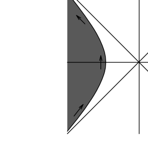
Figure 4.2: Phase space picture of the Fermi sea.

With phase space coordinates the puncture one point function can be written as

$$<P>=\int_{H\leq-\mu}dpd\lambda.$$ (4.22)

The two point function follows from this as

$$<PP>=\frac{\partial}{\partial\mu}\int dpd\lambda\Theta(-\mu-H)$$

$$=\int dpd\lambda\delta(-\mu-H)=\oint_{Fermisurface}.$$ (4.23)

More generally for some operator $O$ consisting of polynomials in $\lambda$ and $p$:

$$<OP>=\oint_{Fermisurface}O.$$ (4.24)

The two point, or $\rho(\mu)$, can also be written as

$$<PP>=\frac{1}{\pi}{\rm Im}\sum_{n}\frac{1}{e_{n}+t_{0}+i\epsilon}$$

$$=\frac{1}{\pi}{\rm Im}\int_{0}^{\infty}dT\sum_{n}<n\mid e^{-T(\mu+H)}\mid n>=\frac{1}{\pi}{\rm Im}\int_{0}^{\infty}dT\int d\lambda G(\lambda,\lambda;T).$$ (4.25)

We see that there are several ways of approaching computations of matrix model correlation functions. One way is to start with the first expression in (4.25). One may then analytically continue to a right side up oscillator. This was the way the original calculation, [42], was done. The sum over the energy eigenvalues becomes a sum over the imaginary energy eigenvalues in a continued right side up. This is also the way in which we will do computations in this thesis. Another approach is to use the path integral formulation, i.e. to use the last representation in (4.25). This was, for nonzero momentum, first done in [58] and extended in [18].

For reference we give the genus expansion of the puncture two point function as obtained in [42]

$$<PP>=-\frac{1}{\pi}{\rm Im}\sum_{n=0}^{\infty}\frac{1}{\frac{i}{2\sqrt{\alpha^{\prime}}}(2n+1)-t_{0}}=-\frac{\sqrt{\alpha^{\prime}}}{\pi}{\rm Re}\psi(\frac{1+i2\sqrt{\alpha^{\prime}}t_{0}}{2})$$

$$=\frac{\sqrt{\alpha^{\prime}}}{\pi}\left(\mid\log\mu\mid+\sum_{n=0}^{\infty}B_{2n}(\frac{1}{2})(-1)^{n}\frac{1}{2n}\frac{1}{(\sqrt{\alpha^{\prime}}t_{0})^{2n}}\right),$$ (4.26)

where $B_{2n}(\frac{1}{2})=(2^{1-2n}-1)B_{2n}$.

This is a good point to reconsider the results of the previous chapter. From the relations derived earlier in this chapter, it follows that for genus one

$$E_{1}=-\frac{1}{24\pi\sqrt{\alpha^{\prime}}}\mid\log\Delta\mid.$$ (4.27)

As we have pointed out this is twice as large as the field theory answer. The explanation is however simple. Recall the matrix model potential and the Fermi sea. The expression (4.26) really presupposes that there are two Fermi seas. One on each side of the top of the potential. Hence there are really two copies of the world, perturbatively disconnected. Clearly this leads to a doubling of the free energy. In the next chapter we will briefly consider a case where there is only one world.

There are several additional comments to be made about the genus 1 partition functions. This will also, in fact throw some light on how special the choice of an inverted harmonic oscillator is.

As discussed in chapter 3 the genus 1 partition function is basically obtained just from the diagram of a single particle closed loop. This we could write as $\sim\int\partial^{2}G(x,x)$, where $G(x,y)=\log\mid x-y\mid$ is the propagator at equal times. $x$ is a space coordinate. This certainly needs some regularization. One possibility is a lattice cutoff $\tilde{L}$ in some finite volume $L$. The result would schematically be

$$E_{1}\sim L(\frac{1}{\tilde{L}^{2}}+\frac{1}{L^{2}})$$ (4.28)

The second term is the $\zeta$ function regularized sum of oscillators in the volume $L$. In the $L\rightarrow\infty$ limit this term is dropped. It is only this second term which is universal, the first one needs some new physics, e.g. the scale of the cutoff, to be determined. The modular invariance of the last chapter is precisely such a prescription. The expression (4.28) looks rather symmetric. In fact, the first term can also be thought of as a $\zeta$ function regularized sum, but now in some “internal” space of volume $\tilde{L}$. We will see in a moment from where this comes in the matrix model.

As noted in [22], the $E_{1}$ can be thought of as arising from insisting that the coincident propagator of the one loop diagram should be defined by normal ordering in $\lambda$ space. When we coordinate transform to $\tau$ space, where $\tau$ is the time of flight for $\lambda$, we pick up a Schwarzian derivative which precisely gives $E_{1}$. The map between $\lambda$ and $\tau$ is $\lambda=\sqrt{\mu}\cosh\tau$ in general. At the top it is $\lambda\sim e^{\tau}$. But this reminds us about a similar situation in conformal field theory where one maps from the plane to the cylinder. There it is well known that the Schwarzian derivative of the map and an explicit sum over modes on the cylinder give the same result. In our case the circumference of the “cylinder” is the imaginary period of $e^{\tau}$, i.e. the time period for oscillations in the continued harmonic oscillator. This is $\tilde{L}$. As we will see later, this period is also related to the quantized momentum of the special states.

This discussion began with a promise that it would say something about the more general models with anharmonic potentials. It is clear that $\tilde{L}$, the characteristic size of the string, is independent of the cosmological constant, either $\mu$ or $\Delta$, only for the harmonic potential. Hence we have $L\sim\log\mu$ and $\tilde{L}\sim 1$. In general the period depends on the amplitude and we have both $L$ and $\tilde{L}$ $\sim\mu^{-k}$ for some positive $k$.

Not only does the effective size of the string depend on the cosmological constant, there is no natural way of keeping the scale of the string and the scale of space very different. This is only one of many strange features of the multi critical models.

4.3 The Special States

In the discussion of the Liouville theory in chapter 2, the special states were introduced.

In the matrix model representation of the theory it is easy to see some of these degrees of freedom. In particular, there exist special operators of zero momentum, which are represented as time independent perturbations of the matrix model potential. These are the analogs of the scaling operators in the one dimensional matrix model. They have the physical effect, in the matrix model, of moving one from one critical point to another. Their correlation functions are easily computed on the sphere and for a general genus surface. In chapter 7 we will investigate these zero momentum correlation functions and show that they obey certain recursion relations which relate all of them to the puncture two point function. We will consider both one particle irreducible and connected amplitudes. The recursion relations allow for computation of any zero momentum correlation function for any genus. They are very similar to the recursion relations for $c<1$ theories and suggest a topological interpretation. We will also rewrite the recursion relations in the form of constraints on the puncture one point function. These constraints obey a Virasoro algebra.

We will then proceed, in chapter 8, to consider the operators of nonzero momentum. The obvious candidate in the matrix model for these operators are the time dependent perturbations of the matrix model potential. We will calculate correlation functions both on the sphere and on a surface of arbitrary genus of such time dependent perturbations. We find that correlation functions of these operators have real poles in the Euclidean momentum, conjugate to the target space variable, at precisely the expected values of the momenta of the special states.

What is the meaning of these special operators in the matrix model? A hint to their meaning is provided by the analysis, [37], of the discrete string. This is the model in which the string is mapped onto a discrete set of points with equal spacing $\epsilon$. It was shown that this model was equivalent to the model where the string is mapped onto a continuous line, as long as $\epsilon<\epsilon_{\rm cr}$, at which point a transition appears to take place. Now this model of triangulated surfaces is the dual of the case where the string is mapped onto a circle of radius $R={1\over\epsilon}$ and the transition is dual to the Kosterlitz-Thouless transition which arises due to the condensation of vortices. We will discuss this a little bit more in chapter 6. One explanation of the equivalence of the continuous and discrete strings, given in [38], is to note that the discretized line can be replaced by a continuous variable $t$ with a periodic potential, $V(t)=\sum_{n}a_{n}\cos({2\pi n\over\epsilon}t)$. The lowest dimension operator in this potential, $n=1$, has undressed conformal dimension $\frac{\alpha^{\prime}}{4}(\frac{2\pi}{\epsilon})^{2}$ and becomes relevant (i.e. of undressed conformal dimension one), when $\epsilon=\epsilon_{\rm cr}=\pi\sqrt{\alpha^{\prime}}$. This is where the phase transition of the discrete string took place. The variable $t$ is forced to take values at the minima of $V(t)$ and the real line is effectively discretized. Now, these terms in the potential correspond precisely to periodic time dependent perturbations of the $c=1$ matrix model and the place where the transition takes place corresponds precisely to one of the special values of the momenta at which the special states occur. Thus we might conjecture that the physical meaning of these operators is that they transform the continuous line into a set of discrete points, with a period given by the inverse of the special values of the momenta — spontaneous punctuation.

As we will see later on, it is not enough to just consider the matrix eigenvalues when identifying the special states. To really be able to see the individual special states one needs to invoke the conjugate momentum. The precise way in which this leads to the $W_{\infty}$ symmetry will be discussed in chapter 9.

Finally it is useful to point out that one important advantage of the analytical continuation approach advocated in [15, 16], is that the special states are given a very clear interpretation. As we will see in more detail in chapter 8, they correspond to resonances in the harmonic oscillator. This is also a reflection of the fact that they are present for Euclidean momenta. Hence to really see them in a Fermi liquid picture, we must use the analytical continuation. This is illustrated in figure 4.3. Now any special state is associated to some periodic ripple on the Fermi surface.

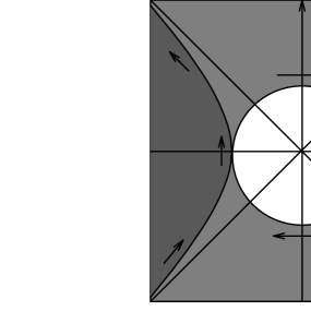
Figure 4.3: Analytical continuation of the phase space picture.

4.4 Summary

In this chapter we have described the $c=1$ matrix model and how it solves many of the problems of formulating a noncritical string theory. Several formulas for calculating correlation functions have been obtained which will be useful in later chapters. We have also encountered the special states which will be of major importance in coming chapters.

Chapter 5 Nonperturbative Effects

5.1 Introduction

In this chapter we will discuss some of the nonperturbative issues of two dimensional string theory. This is really the most remarkable property of the matrix model solution, the possibility of obtaining nonperturbative results. A general discussion of nonperturbative effects in string theory [75] suggests that the $(2g)!$ behavior in (4.26) and the $e^{-1/g_{st}}$ behavior we will find below are generic for closed string theory. This was first observed for the $c=1$ model in [42].

5.2 One World or Two

We will consider an explicit and very simple example as an illustration of what happens nonperturbatively. An extensive treatment can be found in [60]. For our limited purposes we will use other and simpler methods.

Our starting point, as for most cases in this thesis, will be the expression (4.26) for the puncture two point function. Perturbatively each of the terms in the genus expansion can be obtained using the WKB approximation. Since the expansion turns out not to be Borel summable, the summation is not perturbatively determined. Additional information is needed. Roughly speaking, we have the freedom to add terms of the form $e^{-1/g_{st}}$, where $g_{st}$ is the string coupling. Such terms do not show up in the small $g_{st}$ expansion. The two point function as given by (4.26) therefore includes additional nonperturbative information which seems to have been provided by the matrix model. However, as we will see, the choice is not unique.

The following is a simple modification of the matrix model which leads to a nonperturbatively different result. Instead of having just the upside down harmonic oscillator potential, we imagine having an infinite wall erected at the top of the potential. One might say that one has one rather than two worlds. Clearly the WKB expansion, which only feels the potential up to the classical turning point, will be insensitive to this. The wall can only be felt nonperturbatively. The expression for the puncture two point function can be easily adjusted to describe this situation. The effect of the wall is to impose a new boundary condition by forcing the wave functions to be zero at the position of the wall. Hence, rather than summing over all energy eigenstates, we sum only over the odd ones. Therefore, the two point function in the case of the wall is given by

$$<PP>=\frac{1}{\pi}{\rm Re}\sum_{n=odd}\frac{1}{\frac{1}{2\sqrt{\alpha^{\prime}}}(2n+1)+i\beta\mu}=-\frac{\sqrt{\alpha^{\prime}}}{2\pi}{\rm Re}\psi(\frac{3+2\sqrt{\alpha^{\prime}}\beta\mu i}{4}).$$ (5.1)

By the above reasoning we know that this must perturbatively be precisely half of the result without a wall. This can be checked explicitly by using the same kind of expansion as in (4.26) and the Bernoulli polynomial identity $B_{2n}(1/2)=4^{n}B_{2n}(3/4)$. However, nonperturbatively there may be a difference. Let us calculate it. By using the $\psi$ function identities:

$$\psi(2z)=\frac{1}{2}(\psi(z)+\psi(z+\frac{1}{2}))+\log 2\\$$

$$\psi(1-z)=\psi(z)+\pi\cot\pi z,$$ (5.2)

one easily shows

$$\psi(\frac{1+z}{2})=\psi(\frac{3+z}{4})+\log 2-\frac{\pi}{2}\cot(\pi\frac{1+z}{4})+\frac{1}{2}(\psi(\frac{3-z}{4})-\psi(\frac{3+z}{4})).$$ (5.3)

With $z=2\sqrt{\alpha^{\prime}}\beta\mu i$ imaginary it follows

$${\rm Re}\psi(\frac{1+2\sqrt{\alpha^{\prime}}\beta\mu i}{2})={\rm Re}\psi(\frac{3+2\sqrt{\alpha^{\prime}}\beta\mu i}{4})+\log 2-\frac{\pi}{2\cosh\pi\sqrt{\alpha^{\prime}}\beta\mu}.$$ (5.4)

The nonperturbative nature of the difference is obvious. Expanding it for small $e^{-1/g_{st}}$ we find

$$-\pi\sum_{n=0}^{\infty}(-1)^{n}e^{-(2n+1)\pi\sqrt{\alpha^{\prime}}\beta\mu}.$$ (5.5)

This nonperturbative ambiguity can also be understood from an integral representation point of view. We note that

$$\psi^{\prime}(\frac{1+z}{2})=\psi^{\prime}(\frac{1+z}{4})+\frac{1}{2}(\psi^{\prime}(\frac{3+z}{4})-\psi^{\prime}(\frac{1+z}{4})).$$ (5.6)

Using

$$\psi^{\prime}(z)=\int_{0}^{\infty}\frac{te^{-zt}}{1-e^{-t}}$$ (5.7)

one can, by a change of variables $t\rightarrow-t$, prove that for $z=2\sqrt{\alpha^{\prime}}\beta\mu i$

$$\frac{2}{\sqrt{\alpha^{\prime}}}\frac{d}{d\beta\mu}{\rm Re}\psi(\frac{1+z}{4})={\rm Re}\int_{0}^{\infty}\frac{te^{-\frac{1+z}{4}t}}{1-e^{-t}}$$

$$\frac{2}{\sqrt{\alpha^{\prime}}}\frac{d}{d\beta\mu}{\rm Re}\psi(\frac{3+z}{4})={\rm Re}\int_{0}^{-\infty}\frac{te^{-\frac{1+z}{4}t}}{1-e^{-t}}.$$ (5.8)

The integrands are the same, but the contours differ. One is the real line from $0$ to $+\infty$, the other one the real line from $0$ to $-\infty$. If we rotate one contour into the other, we pick up residues from the poles along the imaginary axis, this precisely gives (5.5).

Hence we have established the nonperturbative nature of the difference between one and two worlds.

5.3 Instantons

It would be nice to have a more physical picture of the nonperturbative string theory. We will try to achieve this below.

Nonperturbative effects are in general associated with instantons. In this case we have eigenvalue fermions at the Fermi surface tunneling through the upside down potential. Without the wall, the instanton action for one fermion tunneling through is obtained from the Euclidean action $\beta\int dt(\frac{1}{2}\dot{\lambda}^{2}-\frac{1}{2\alpha^{\prime}}\lambda^{2})$ evaluated for the classical tunneling solution of energy $\mu$. We also need to subtract the action for a fermion not doing any tunneling, i.e. just sitting at $\mu=\frac{1}{2\alpha^{\prime}}\lambda^{2}$. The result is

$$\beta\int_{-\sqrt{2\alpha^{\prime}\mu}}^{\sqrt{2\alpha^{\prime}\mu}}d\lambda\sqrt{2\mu-\frac{1}{\alpha^{\prime}}\lambda^{2}}=\sqrt{\alpha^{\prime}}\pi\mu\beta.$$ (5.9)

Now, for two worlds the instantons correspond to tunnelings through the potential and back again. The leading instanton contribution to the propagator, $G(\lambda,\lambda)$, has then the weight

$$e^{-2\sqrt{\alpha^{\prime}}\pi\mu\beta}.$$ (5.10)

Considering the integral representation of $Re\psi(\frac{1+z}{2})$ we indeed note poles leading to such contributions.

Let us turn to the case of one world. We write the two world propagator as a sum over even and odd (i.e. one world) parts $G(\lambda,\lambda)=G_{e}(\lambda,\lambda)+G_{o}(\lambda,\lambda)$. Then $G(\lambda,-\lambda)=G_{e}(\lambda,\lambda)-G_{o}(\lambda,\lambda)$ and from that $G(\lambda,\lambda)-2G_{o}(\lambda,\lambda)=G(\lambda,-\lambda)$. The leading contribution to $G(\lambda,-\lambda)$ is a tunneling solution through the potential barrier, but not back again and hence of order

$$e^{-\sqrt{\alpha^{\prime}}\pi\mu\beta}.$$ (5.11)

This verifies and illustrates the calculations in the previous section.

5.4 Summary

Clearly much remains to be done concerning the nonperturbative aspects of the two dimensional string. The important contribution of the matrix models is a laboratory where we can check our understanding of nonperturbative string physics. As we have seen above, the nonperturbative effects have a rather simple interpretation in terms of single eigenvalue tunneling. What remains to be obtained is a clear picture of what happens in a string language. One possibility, which has been raised in the past, is that by clarifying this issue, one could eventually find the “real meaning” of string theory. Perhaps this will involve concepts which transcend the traditional genus expansion.

Chapter 6 String Theory at Finite Radius

6.1 Introduction

In this chapter we will consider the two dimensional string theory with compactified time on some radius $R$. In other words, string theory at finite temperature. This has been extensively treated in [51]. We will however use another and very simple approach to reproduce some of these results. It is our feeling that the method below may provide some useful insights into the basics of the matrix model description of string theory.

As mentioned in chapter 4, it is not really correct to ignore the angular parts of the matrix integral for finite $R$, [37, 38]. The angular parts are related to vortices. These vortices are found to cause a phase transition at a radius of twice the self dual radius, this is the Kosterlitz-Thouless transition. As described in [37, 38] the transition is caused by operators $\cos(\frac{R}{\alpha^{\prime}}(X_{R}-X_{L}))$, which create vortices and become relevant at $R=2\sqrt{\alpha^{\prime}}$. Below this radius the vortices destroy the string world sheet. Therefore, the calculation which we will consider below, assumes automatically that vortices are excluded for some reason. It is not clear if this is a physically reasonable assumption.

In the presence of vortices the target space duality of string theory under $R\rightarrow\alpha^{\prime}/R$ is explicitly broken. One might comment, [64], that there is a dual object to vortices, “spikes”, which tend to condense for large $R$, more precisely $R>\frac{1}{2}\sqrt{\alpha^{\prime}}$. The spikes are created by $\cos(\frac{\alpha^{\prime}}{R}(X_{R}+X_{L}))$. This is the punctuation phenomenon we discussed at the end of chapter 4. If we include such spikes, duality is restored but to the price of having an instable theory for any radius! Luckily, spikes may be forbidden simply by imposing translational invariance since the operators which excite them, break this invariance. This is not true for the vortices.

The fact remains, however, that duality is broken. Clearly, this could have far reaching consequences also for higher dimensional string theories. The argument leading to the Kosterlitz-Thouless transition is, after all, a very general one. It is just, as usual, a matter of competition between energy and entropy. To see this, one has to introduce a cutoff, like the triangulation of the matrix model. As the cutoff is removed, the energy of a vortex goes to infinity but at the same time the number of possible vortices also rises. The temperature decides which one will win.

Hence we might learn from the matrix model two dimensional string theory to be careful when we apply concepts like duality to draw general string theory conclusions. We might be using a principle not realized in a realistic theory.

With this in mind, let us now give a very simple finite radius calculation.

6.2 A Simple Example

Let us derive a finite radius expression for the puncture two point function. To do that, let us consider the fermionic field theory action on finite radius

$$S=\int_{0}^{2\pi R}dtd\lambda[\frac{1}{\beta}\dot{\psi}^{\dagger}\psi+\frac{1}{\beta^{2}}\frac{\partial\psi^{\dagger}}{\partial\lambda}\frac{\partial\psi}{\partial\lambda}+U(\lambda)\psi^{\dagger}\psi].$$ (6.1)

The path integral,

$$Z=\int{\cal D}\psi{\cal D}\psi^{\dagger}e^{-\beta S},$$ (6.2)

is easily done by expanding $\psi$ in eigenfunctions of $\frac{\partial}{\partial t}$ in time and eigenfunctions of the harmonic oscillator in the $\lambda$ coordinate. The eigenvalues are $\frac{2m+1}{2R}$ for the time part since we need anti periodic boundary conditions for the fermions. For the harmonic oscillator part we have the standard $\frac{1}{2\sqrt{\alpha^{\prime}}}(2n+1)$. There is also the energy shift $t_{0}=\beta\mu$. A standard evaluation of the logarithm of the path integral, giving a logarithm of a determinant and hence a trace of a logarithm of the eigenvalues, then yields the following expression for the two point function

$$<PP>=\frac{1}{\pi R}{\rm Im}\sum_{n,m}\frac{1}{(\frac{1}{2\sqrt{\alpha^{\prime}}}(2n+1)i+\frac{(2m+1)i}{2R}-t_{0})^{2}}.$$ (6.3)

If the sum over $m$ is performed the result of [37] is recovered. Using this expression a general correlation function can be obtained through perturbation theory in the same way as for the $R=\infty$ case extensively treated elsewhere in this thesis.

Once this is established, it is also easy to write down a recipe which converts the ordinary $R=\infty$ two point function into the finite $R$ case. The point of doing so is that this procedure, as is easily seen, commutes with the variations giving other correlation functions. As we will see, this procedure is precisely the one derived independently in [51].

In words, what one has to do is to take one $t_{0}$ derivative and then sum over all shifts $\frac{(2m+1)i}{2R}$ in the $t_{0}$ variable. The shift can be written down using the identity

$$e^{z\frac{\partial}{\partial x}}f(x)=f(x+z)$$ (6.4)

for any function $f(x)$. We get

$$(1-e^{-\frac{i}{R}\frac{\partial}{\partial t_{0}}})\sum_{n,m}\frac{1}{(\frac{1}{2\sqrt{\alpha^{\prime}}}(2n+1)i+\frac{(2m+1)i}{2R}-t_{0})^{2}}=\sum_{n}\frac{1}{(\frac{1}{2\sqrt{\alpha^{\prime}}}(2n+1)i+\frac{i}{2R}-t_{0})^{2}}$$

$$=e^{-\frac{i}{2R}\frac{\partial}{\partial t_{0}}}\sum_{n}\frac{1}{(\frac{1}{2\sqrt{\alpha^{\prime}}}(2n+1)i-t_{0})^{2}}=e^{-\frac{i}{2R}\frac{\partial}{\partial t_{0}}}\frac{\partial}{\partial t_{0}}\sum_{n}\frac{1}{\frac{1}{2\sqrt{\alpha^{\prime}}}(2n+1)i-t_{0}}.$$ (6.5)

Hence

$$\frac{1}{R}\sum_{n,m}\frac{1}{(\frac{1}{2\sqrt{\alpha^{\prime}}}(2n+1)i+\frac{(2m+1)i}{2R}-t_{0})^{2}}=\frac{\frac{1}{R}\frac{\partial}{\partial t_{0}}}{e^{\frac{i}{2R}\frac{\partial}{\partial t_{0}}}-e^{-\frac{i}{2R}\frac{\partial}{\partial t_{0}}}}\sum_{n}\frac{1}{\frac{1}{2\sqrt{\alpha^{\prime}}}(2n+1)i-t_{0}}.$$ (6.6)

This verifies the result of [51] using a different method.

There are some interesting features of this derivation. Duality is very explicit in the expression (6.3). That is, if we do not care about the vortices as discussed in the introduction. We can in fact learn a bit about how it is realized in the matrix model. Apparently duality relies on the fact that the eigenvalue spectrum of a harmonic oscillator is the same as for a fermion with anti periodic boundary conditions in a box! Clearly one cannot expect duality to hold in any matrix model. In general a nonharmonic potential would have nonequally spaced eigenvalues and hence break duality.

Curiously, by the same reasoning, many correlation functions will break duality. This is not surprising for nonzero momentum correlation functions. However, the above expressions suggest this to be the case even at zero momentum for the special states.

6.3 Summary

In this chapter a simplified derivation of some results for finite radius has been given. We have indicated how duality is realized in the matrix model. An important observation is that naïve duality is not expected to hold in a general matrix model.

Chapter 7 Zero Momentum Correlation Functions

7.1 Introduction

A first exercise in the two dimensional string theory is the calculation of zero momentum correlation functions. Clearly this is the simplest thing to do. Such calculations will be described in this chapter. We will, apart from some comments towards the end of the chapter, limit ourselves to powers of the matrix model eigenvalue. The conjugate momentum will be introduced in later chapters. One of the main results of this chapter will be a set of recursion relations for these correlation functions.

7.2 The Gelfand-Dikii Equation

Let us briefly recall the basics of the matrix model approach to $c=1$ quantum gravity or two dimensional string theory as described in chapter 4. We will limit ourselves to the uncompactified case. The partition function is given by

$$\int{\cal D}\phi e^{-\beta\int Tr(\frac{1}{2}\dot{\phi}^{2}+U(\phi))dt},$$ (7.1)

where $\phi$ is a hermitean $N\times N$ matrix. As shown in [7], the angular variables may be integrated out to leave only the $N$ eigenvalues. They correspond to $N$ fermions in the potential $U$. Below we will consider correlation functions of precisely these eigenvalues.

As we have seen, the density of states, $\rho$, in the potential, is the same as the 1PI puncture two point function and hence a very interesting and basic quantity in the theory. In the coordinate basis it can be written as

$$\rho(\mu_{F})=\frac{1}{\pi\beta}{\rm Im}\int d\lambda<\lambda\mid\frac{1}{\hat{H}-\mu_{F}-i\epsilon}\mid\lambda>$$ (7.2)

By investigating some properties of this expression, we will be able to extract information about zero momentum correlation functions of the matrix eigenvalue variable.

We begin by defining the function

$$R(\lambda)=<\lambda\mid\frac{1}{-\frac{1}{2}\nabla_{\lambda}^{2}+U(\lambda)}\mid\lambda>,$$ (7.3)

i.e. the diagonal component of the resolvent. This function obeys the nonlinear Gelfand-Dikii equation [30]:

$$-2RR^{\prime\prime}+(R^{\prime})^{2}+8U(\lambda)R^{2}=4.$$ (7.4)

Here $\lambda$ is shifted so that the maximum of the potential is at the origin. We have also shifted $U$ by $\mu_{F}=\mu_{c}-\mu$. In the double scaling limit we expand $U(\lambda)$ around its maximum and rescale the coordinate. If $U(\lambda)\sim\lambda^{n}$, then $\lambda\sim\beta^{\frac{2}{n+2}}$. In the following it is assumed that all quantities are rescaled in the appropriate fashion.

The correlation functions we are going to calculate will be correlation functions of time independent perturbations, $\lambda^{k}$, around the top of the potential. The corresponding operators we call $O_{k}$. They are essentially the operators ${1\over N}{\rm Tr}[\phi-\phi_{c}]^{k}$. To perform the calculations we include in $U$ general perturbations $\lambda^{k}$ coupled to sources $t_{k}$, which we later will vary. Taking one derivative of (7.4) gives the linearized version of the Gelfand-Dikii equation,

$$-\frac{1}{2}R^{\prime\prime\prime}+4UR^{\prime}+2U^{\prime}R=0.$$ (7.5)

This formula is also easily verified by using $R(\lambda)=\sum_{n=0}^{\infty}\frac{\psi^{\dagger}_{n}(\lambda)\psi_{n}(\lambda)}{E_{n}}$, and the Schrödinger equation for the energy eigenfunctions $\psi_{n}(\lambda)$. Note that we are dealing with an inverted potential and the $E_{n}$’s are therefore, in general, complex. It is this linearized version of the Gelfand-Dikii equation which we will exploit in the following in order to get information about the correlation functions of the theory.

The resolvent $R(\lambda)$ determines the density of states,

$$\rho(\mu)=\frac{1}{\pi}{\rm Im}\int R(\lambda)d\lambda,$$ (7.6)

which is also the puncture two point function $<PP>$. Other two point functions can be obtained by taking the moments of $R$,

$$<O_{k}P>=\frac{1}{\pi}{\rm Im}\int\lambda^{k}R(\lambda)d\lambda.$$ (7.7)

These amplitudes are one particle irreducible (1PI) with respect to the puncture.

Some comments on the integration region are in order. There are essentially two different cases depending on whether we have one or two worlds as explained in chapter 4. From the point of view of the WKB approximation we should integrate only up to the top of of the potential, i.e. from $-\infty$ to zero in the case of one world. With two worlds, we should integrate all the way from $-\infty$ to $+\infty$. This is effectively a doubling of the system. At a critical point, where we just have a leading even power contribution to $U(\lambda)$, $R(\lambda)$ is clearly even. This immediately implies that, with two worlds, (7.7) is zero for $k$ odd. For the quadratic critical point this is true also with one world. The above integral for an odd operator turns out to be real and therefore gives no contribution to the imaginary part.

7.3 1PI Recursion Relations

We will now use the linearized Gelfand-Dikii equation to derive recursion relations for the 1PI amplitudes. We start with (7.5) for a general potential

$$U(\lambda)=\sum_{p=0}^{\infty}t_{p}\lambda^{p}.$$ (7.8)

The $t_{p}$’s will act as sources for the $O_{p}$ operators. We will later restrict ourselves to the quadratic critical point

$$t_{i}=0\hskip 10.00002pt\forall i\neq 0,2\hskip 20.00003ptt_{0}=\beta\mu\hskip 20.00003ptt_{2}=-\frac{1}{2\alpha^{\prime}}<0.$$ (7.9)

We then compute the $\lambda^{k+1}$ moment of (7.5), obtaining

$$-\frac{1}{2}(k+1)k(k-1)<O_{k-2}P>+2\sum_{p=0}^{\infty}t_{p}(2k+p+2)<O_{k+p}P>=0.$$ (7.10)

To obtain this, we have made repeated partial integrations and discarded boundary terms at infinity which do not contribute to the singular part of the correlation functions. In the case of one rather than two worlds, one might worry about boundary terms at $\lambda=0$. However these are real, as follows immediately from the WKB expansion of $R(\lambda)$ in terms of $\sqrt{U(\lambda)}$. Hence, they do not contribute to the imaginary parts of the integrals, which give the correlation functions. Using $<O_{p}...>=\frac{\partial}{\partial t_{p}}<...>$ we may take $t_{p}$ ($p>0$) derivatives of (7.10) to derive

$$\begin{array}[]{c}-\frac{1}{2}(k-1)k(k+1)<O_{k-2}O_{k_{1}}\dots O_{k_{p-1}}P>\\ \\ +4t_{0}(k+1)<O_{k}O_{k_{1}}\dots O_{k_{p-1}}P>+4t_{2}(k+2)<O_{k+2}O_{k_{1}}\dots O_{k_{p-1}}P>\\ \\ +2\sum_{i=1}^{p-1}(2k+k_{i}+2)<O_{k+k_{i}}O_{k_{1}}...\hat{O}_{k_{i}}...O_{k_{p-1}}P>=0.\end{array}$$ (7.11)

For simplicity we have chosen the quadratic critical point of (7.9). When we take the derivatives, $t_{0}=\beta\mu$ is kept constant. This is because $\beta\mu$ is the nonamputated puncture one point function and we are considering 1PI amplitudes.

With this recursion relation any zero momentum correlation function for arbitrary genus may be expressed in terms of the puncture two point function. Using the fact that the genus g contribution to the correlation function depends on $t_{0}$ according to $<O_{k_{0}}...O_{k_{p-1}}P>_{g}\sim t_{0}^{\frac{1}{2}\sum_{i=0}^{i=p-1}k_{i}+1-p-2g}$, we can write a formula where we exhibit the explicit genus dependence:

$$\begin{array}[]{c}-\frac{1}{2}(k-1)k(k+1)<O_{k-2}O_{k_{1}}...O_{k_{p-1}}P>_{g-1}\\ \\ +4t_{0}(k+1)<O_{k}O_{k_{1}}...O_{k_{p-1}}P>_{g}+4t_{2}(k+2)<O_{k+2}O_{k_{1}}...O_{k_{p-1}}P>_{g}\\ \\ +2\sum_{i=1}^{p-1}(2k+k_{i}+2)<O_{k+k_{i}}O_{k_{1}}...\hat{O}_{k_{i}}...O_{k_{p-1}}P>_{g}=0,\end{array}$$ (7.12)

where the first term is understood to be zero for $g=0$.

These recursion relations are similar to the ones that exist for $c<1$. The genus mixing first term looks like a contribution from a pinched handle, while the last term corresponds to contact terms between operators. What is lacking are the quadratic terms which arise when the surface is pinched into two separate surfaces. The reason these are absent is that we have considered 1PI amplitudes with respect to the puncture which precisely excludes such terms. The corresponding recursion relations for connected amplitudes will be derived in the next section.

It is straightforward to check that the results for the sphere, obtained in [39] using different methods:

$$<O_{k_{0}}O_{k_{1}}...O_{k_{p-1}}P>_{0}=-\mid\ln\mu\mid\left(\begin{array}[]{c}2\Sigma\\ \Sigma\end{array}\right)\frac{1}{\pi\sqrt{2|t_{2}|}}\frac{1}{(-4t_{2})^{\Sigma}}\frac{\partial^{p-1}}{\partial t_{0}^{p-1}}t_{0}^{\Sigma},$$ (7.13)

for even $k_{i}$’s, satisfy (7.12), where $\Sigma=\frac{1}{2}\sum_{i=0}^{p-1}k_{i}$. Note that the first term of (7.12) does not contribute. The factors of $t_{2}$ assure that $t_{2}$ derivatives generate $O_{2}$ insertions. Note that, in using the recursion relations, we have to fix the normalization $<PP>_{0}=-\frac{1}{2\pi}|\ln\mu|$ for $t_{2}=-2$ ($\alpha^{\prime}=1/4$). The formula is also true for odd $k_{i}$’s, unless $2\Sigma$ is odd, in which case the correlation functions are zero. This follows from (7.11) for $k=-1$, $p=1$ which states that $<O_{1}P>=0$, as we discussed in the previous section.

Let us explicitly evaluate a simple example of a correlation function at arbitrary genus. We consider the operator $O_{2}$. If we put $k=0$ in (7.12) the first term vanishes, i.e. no genus mixing, and we are left with

$$\begin{array}[]{c}8t_{2}<O_{2}O_{k_{1}}...O_{k_{p-1}}P>_{g}\\ \\ +4t_{0}<O_{k_{1}}...O_{k_{p-1}}PP>_{g}+(4(p-1)+4\Sigma)<O_{k_{1}}...O_{k_{p-1}}P>_{g}=0,\end{array}$$ (7.14)

i.e.

$$2t_{2}<O_{2}O_{k_{1}}...O_{k_{p-1}}P>_{g}=-(p-1+\Sigma+t_{0}\frac{\partial}{\partial t_{0}})<O_{k_{1}}...O_{k_{p-1}}P>_{g}.$$ (7.15)

Since $<O_{k_{1}}...O_{k_{p-1}}P>_{g}\sim t_{0}^{\Sigma+2-p-2g}$ we find

$$2t_{2}<O_{2}O_{k_{1}}...O_{k_{p-1}}P>_{g}=-(2\Sigma+1-2g)<O_{k_{1}}...O_{k_{p-1}}P>_{g}.$$ (7.16)

This expression is similar to the dilaton equation obtained in [26] for topological gravity. In particular

$$<\overbrace{O_{2}...O_{2}}^{n}>_{g}=\bigl{(}\frac{-1}{2t_{2}}\bigr{)}^{n}\prod_{p=1}^{n}(2p-1-2g)<>_{g}.$$ (7.17)

Note that $<O_{2}>_{g}=\frac{1}{2t_{2}}(2g-1)<>_{g}$, which suggests that $O_{2}$ is almost, but not quite, the dilaton.

7.4 Connected Recursion Relations

Let us now derive recursion relations for connected amplitudes. This is not more difficult than in the 1PI case. In the case of the 1PI (with respect to the puncture) amplitudes the generating functional, $\Gamma$, depends on the nonpuncture sources $t_{k}$ ($k\geq 1$) and the nonamputated puncture one point function $t_{0}=\beta\mu$. $t_{0}$ is kept constant while the other $t_{k}$’s vary. The generating functional for connected amplitudes, the vacuum energy $E$, depends instead on the $t_{k}$ ($k\geq 1$) and $\Delta$, the puncture source, i.e. the cosmological constant. In this case $\Delta$ is kept constant when the $t_{k}$’s vary and $t_{0}$ is a function of the $t_{k}$’s. $\Delta$ is also the amputated one point function. $\Gamma$ and $E$ are related by the Legendre transform

$$E(\Delta)=\beta^{2}\Delta\mu-\Gamma(\mu).$$ (7.18)

We have

$$\beta\Delta=\frac{\partial\Gamma}{\partial(\beta\mu)},\hskip 20.00003pt\beta\mu=\frac{\partial E}{\partial(\beta\Delta)},\hskip 20.00003pt\frac{\partial^{2}E}{\partial t_{k}\partial(\beta\Delta)}=-\frac{\partial\mu}{\partial\Delta}\frac{\partial^{2}\Gamma}{\partial t_{k}\partial(\beta\mu)},$$ (7.19)

as a consequence of

$$0=\frac{d\mu}{dt_{k}}=\frac{\partial\mu}{\partial t_{k}}+\frac{\partial\mu}{\partial\Delta}\frac{\partial\Delta}{\partial t_{k}}.$$ (7.20)

The 1PI and connected two point functions are simply proportional to each other. The same recursion relation is valid. The difference comes when we take $t_{k}$ derivatives to obtain higher point functions. For connected diagrams $t_{0}=\beta\mu$ is no longer to be kept constant. The resulting recursion relations are no longer linear but rather quadratic

$$\begin{array}[]{c}{-\frac{1}{2}(k+1)k(k-1)<O_{k-2}O_{k_{1}}...O_{k_{p-1}}P>_{c}+2t_{2}(2k+4)<O_{k+2}O_{k_{1}}...O_{k_{p-1}}P>_{c}}\\ \\ +4(k+1)\sum_{i\in k}<O_{i_{1}}...O_{i_{n}}P>_{c}<O_{k}O_{i_{n+1}}...O_{i_{p-1}}P>_{c}\\ \\ +2\sum_{i=1}^{p-1}(2k+k_{i}+2)<O_{k+k_{i}}O_{k_{1}}...\hat{O}_{k_{i}}...O_{k_{p-1}}P>_{c}=0.\end{array}$$ (7.21)

Note that $t_{0}=<P>_{c}$. We recognize an extra term suggestive of a surface pinching into two. If we extract the explicit genus dependence we find

$$\begin{array}[]{c}-\frac{1}{2}(k+1)k(k-1)<O_{k-2}O_{k_{1}}...O_{k_{p-1}}P>_{c,g-1}\\ \\ +4(k+1)\sum_{g_{1}+g_{2}=g}\sum_{i\in k}<O_{i_{1}}...O_{i_{n}}P>_{c,g_{1}}<O_{k}O_{i_{n+1}}...O_{i_{p-1}}P>_{c,g_{2}}\\ \\ +4t_{2}(k+2)<O_{k+2}O_{k_{1}}...O_{k_{p-1}}P>_{c,g}\\ \\ +2\sum_{i=1}^{p-1}(2k+k_{i}+2)<O_{k+k_{i}}O_{k_{1}}...\hat{O}_{k_{i}}...O_{k_{p-1}}P>_{c,g}=0.\end{array}$$ (7.22)

This structure is very similar to the one encountered in $c<1$ theories [26].

All connected amplitudes may also be built by using the 1PI building blocks. Let us consider a simple example. Consider

$$<O_{k}P>_{c}=-\frac{\partial\mu}{\partial\Delta}<O_{k}P>=-\frac{1}{\rho}<O_{k}P>.$$ (7.23)

The $1/\rho$ prefactor simply adds an external propagator as it should. Now take a $\frac{\partial}{\partial t_{l}}\mid_{\Delta=const}$ derivative. We get

$$\begin{array}[]{c}<O_{k}O_{l}P>_{c}=(\frac{1}{\rho^{2}}\frac{\partial\rho}{\partial t_{l}}+\frac{1}{\rho^{2}}\frac{\partial\rho}{\partial\mu}\frac{\partial\mu}{\partial t_{l}})<O_{k}P>\\ \\ -\frac{1}{\rho}(<O_{k}O_{l}P>+\frac{\partial\mu}{\partial t_{l}}<O_{k}PP>).\end{array}$$ (7.24)

Now use $\frac{\partial\Delta}{\partial t_{l}}+\frac{\partial\Delta}{\partial\mu}\frac{\partial\mu}{\partial t_{l}}=0$ to obtain

$$\begin{array}[]{c}<O_{k}O_{l}P>_{c}=\frac{1}{\rho^{2}}<O_{l}PP><PO_{k}>-\frac{1}{\rho^{3}}<O_{k}P><PPP><PO_{l}>\\ \\ -\frac{1}{\rho}<O_{l}O_{k}P>+\frac{1}{\rho^{2}}<O_{l}P><PPO_{k}>.\end{array}$$ (7.25)

It is easily checked that this expression indeed obeys (7.21) using the recursion relations for the 1PI amplitudes. The $1/\rho$ factors provide external and internal propagators where needed.

7.5 Virasoro Constraints

There is an interesting way of rewriting the recursion relations (7.10), which explains where they really come from. They are simply equivalent to

$$L_{k}<P>=0\hskip 20.00003pt\forall k\geq-1,$$ (7.26)

where

$$L_{k}=-\frac{1}{4}(k+1)k(k-1)\frac{\partial}{\partial t_{k-2}}+\sum_{p=0}^{\infty}t_{p}(2k+p+2)\frac{\partial}{\partial t_{p+k}}.$$ (7.27)

It is straightforward to verify that the $L_{k}$’s obey a Virasoro algebra

$$[L_{n},L_{m}]=(n-m)L_{n+m}.$$ (7.28)

The Virasoro generators can be understood as representing the algebra of coordinate transformations in the Liouville coordinate, i.e. $L_{k-1}\sim\lambda^{k}\frac{\partial}{\partial\lambda}$. Let us see how this works. In the full quantum treatment, it is convenient to use the matrix eigenvalue $\lambda$ and its conjugate momentum $p$. The generator of the coordinate transformation is then $p\lambda^{k}$. One can convince oneself that one need not worry about different orderings in this case. Acting on the Hamiltonian we find two parts,

$$[p\lambda^{k},U(\lambda)]=\lambda^{k}\frac{\partial U}{\partial\lambda}$$ (7.29)

and

$$[p\lambda^{k},p^{2}]=k(\lambda^{k-1}p^{2}+p^{2}\lambda^{k-1})-\frac{k}{2}(k-1)(k-2)\lambda^{k-3}.$$ (7.30)

When this is evaluated at the Fermi surface in accordance with the variational prescription of (4.23) and (4.24), the $\frac{p^{2}}{2}$ gives a $U(\lambda)$. Hence

$$<(-\frac{1}{4}k(k-1)(k-2)\lambda^{k-3}+2k\lambda^{k-1}U(\lambda)+\lambda^{k}\frac{\partial U}{\partial\lambda})P>=0$$ (7.31)

which is precisely equal to (7.10).

Unfortunately, the $L_{-1}$ constraint for the quadratic critical point is quite trivial

$$L_{-1}<P>=2t_{2}<O_{1}P>=0.$$ (7.32)

It does not seem to yield a string equation determining $<PP>$, unlike the case for the $c<1$ models, [26].

A natural generalization is obviously to consider general transformations $p^{n}\lambda^{m}$. As far as $\lambda^{k}$ correlation functions goes, this will not give anything new. The constraints one obtains are simply linear combinations of the old ones. Although, of course, they represent the full algebra not only the Virasoro part.

7.6 Summary

In this chapter we have seen how to obtain recursion relations for both 1PI and connected zero momentum correlation functions. With the help of these, any zero momentum correlation function for any genus may be calculated, once we know the puncture two point function. The recursion relations were furthermore found to correspond to coordinate transformations in the Liouville coordinate. This was the reason why our recursion relations could be expressed as constraints obeying a Virasoro algebra. The presence of the Virasoro algebra, and as we already have noted, a full $W_{\infty}$ algebra, is of utmost importance. We will in chapter nine and ten take full advantage of this algebra.

By adding time independent operators to the potential the critical behavior may change. The recursion relations and their Virasoro representation should be useful for studying such other critical points, different from the ordinary quadratic. They should also describe the flows between different critical points. Although it is not clear how to identify these new theories, it is easy to extract some information about them. The Virasoro constraints which we have derived are valid for any potential and provide relations between different correlation functions.

As we have seen, the recursion relations do not determine $<PP>$. This has to be specified independently, before the recursion relations can determine all other correlation functions. In general, when we consider some nonquadratic potential, more data need to be specified. For a theory with a $\lambda^{2n}$ as the leading term in the potential, we will need to specify $<PP>$, $<PO_{1}>$,…,$<PO_{2n-2}>$. The correlation $<PO_{2n-1}>$ is always zero. The scaling of $<PP>$ can be derived directly from the WKB approximation and is given by $\mu^{1/2n-1/2}$.

So much for zero momentum correlation functions. In the next chapter we will generalize to nonzero momentum. While doing so, the importance of the special states will become even clearer.

Chapter 8 Nonzero Momentum Correlation Functions

8.1 Introduction

Let us now consider the matrix model and its special states, also for nonzero momentum.

As we have seen the natural candidates for special state correlation functions are correlation functions of powers of the matrix model eigenvalues. Such objects were studied in [15] and the expected poles for discrete momenta were found. In this chapter we will extend some of the results of [15] and the previous chapter, for Ward identities. In particular, we will find that the recursion relation (7.10) is in fact the Wheeler de Witt equation for the two dimensional world sheet quantum gravity.

The recent developments revealing the $W_{\infty}$ symmetries indicate however that this is not the whole story. One should also consider correlation functions involving powers of the conjugate momentum. This we will do in the next chapter, where we will show the existence of this $W_{\infty}$ symmetry which will greatly simplify the subsequent calculations.

8.2 The Wheeler de Witt Equation

Ward identities for correlation functions are in general obtained by changes of variables in the path integral. Examples of such Ward identities were obtained in the last chapter from simple coordinate changes in the matrix eigenvalue. They can be thought of as generated by commutators, or classically, i.e. on the sphere, Poisson brackets with $p\lambda^{m}$. They obviously obey a Virasoro algebra, which is part of a $W_{\infty}$ algebra generated by all monomials $p^{n}\lambda^{m}$. We may also introduce time dependence and consider generators with certain momenta $q$, i.e. $p^{n}\lambda^{m}e^{iqt}$. Let us, as an example, make a $p\lambda^{k}e^{iqt}$ variation of the one puncture function.

As we saw in chapter three, the two puncture function is schematically given by

$$<PP>=\frac{1}{\pi}{\rm Im}\int_{0}^{\infty}dT\int d\lambda G(\lambda,\lambda;T),$$ (8.1)

where the calculation is done at the Fermi surface. We will shift its energy to zero, hence putting the Fermi energy as a constant term in the potential. $G$ is the path integral given by

$$G(\lambda_{1},\lambda_{2})=\int_{\lambda_{1}}^{\lambda_{2}}[dpd\lambda]e^{-\beta\int dt(p\dot{\lambda}-\frac{1}{2}p^{2}+U(\lambda))},$$ (8.2)

in Euclidean time, where $U(\lambda)=\sum_{p}t_{p}\lambda^{p}$ is the potential. The variation of the partition function would have involved a sum over all states in the Fermi sea up to the Fermi level. By inserting a puncture, i.e. taking a derivative with respect to the Fermi energy as in the last chapter, we restrict ourselves to the Fermi surface. Next we perform the variation of $<P>$. The measure, as given by (8.2), is invariant under the change of variables. (Clearly, we are not supposed to differentiate with respect to $t$ when changing variables in the measure.) The change in the action gives rise to the following identity among two point functions

$$<(\int dt(iq\lambda^{k}p+k\lambda^{k-1}p^{2}+\frac{\partial U}{\partial\lambda}\lambda^{k})e^{iqt})T>=0.$$ (8.3)

The puncture is now a tachyon, T, carrying away the momentum. The piece with a single $p$ is evaluated by integrating over $p$ in the path integral, obtaining a $\dot{\lambda}$ which then is partially integrated. We then switch to a Hamiltonian formulation, remembering that we should use Weyl ordering. We finally obtain

$$-\frac{1}{4}k(k-1)(k-2)<O_{k-3}P>_{g-1}+\sum_{p}(2k+p)t_{p}<O_{p+k-1}P>_{g}=0,$$ (8.4)

to all genus at zero momentum, as in the last chapter, and

$$\sum_{p}(2k+p)t_{p}<O_{p+k-1}T>_{q,g}+\frac{q^{2}}{1+k}<O_{k+1}T>_{q,g}=0$$ (8.5)

on the sphere for nonzero momentum. The combined case is somewhat more complicated due to the need of taking an imaginary part and an effective imaginary shift $iq$ in $t_{0}$, relevant for higher genus. We will not consider this any further. In these equations $q$ indicates momentum and $g$ genus. We have introduced the notation $O_{k}$ for $\lambda^{k}$. The different genus for the first term in (8.4) is due to a $p$, $\lambda$ commutator which arises when we want to evaluate the $p^{2}$ against the wave function of the Fermi surface. This gives an $\hbar$, which is the same as the genus coupling constant. Following [58] we may define the loop operator given by

$$w(l)=e^{l\lambda}.$$ (8.6)

It corresponds to cutting out a hole in the surface with a boundary of length $l$. The reason is the following. If we insert a power $n$ of the original matrix variable $\phi$ on the surface this creates a little hole, the length of the boundary being proportional to $n$ (the number of legs) and the lattice spacing $a$. For fixed $n$ the length clearly shrinks to zero in the double scaling limit. To get a finite length we must also take $n$ to infinity. Introducing $\lambda$ as the eigenvalues $m$ of $\phi$ expanded around the top of the potential, we find in the double scaling limit

$$m^{n}\sim(1+a\lambda)^{l/a}\rightarrow e^{l\lambda}.$$ (8.7)

We may then Fourier transform to obtain a differential equation in the loop length. We get

$$[\sum_{p}t_{p}(l^{2}\frac{\partial^{p}}{\partial l^{p}}+\frac{p}{2}l\frac{\partial^{p-1}}{\partial l^{p-1}})+t_{0}l^{2}-l^{4}]<w(l)T>=0$$ (8.8)

at zero momentum and

$$[\sum_{p}t_{p}(l^{2}\frac{\partial^{p}}{\partial l^{p}}+\frac{p}{2}l\frac{\partial^{p-1}}{\partial l^{p-1}})+t_{0}l^{2}+q^{2}]<w(l)T>=0$$ (8.9)

on the sphere. The $l^{4}$ term is of order one higher in the string coupling and do not contribute on the sphere. $t_{0}$ is the Fermi energy $\mu$ with the appropriate number of $\beta$’s absorbed. In the case of the usual harmonic oscillator potential, where $t_{0}=\beta\mu$, the resulting equations are in fact the Wheeler de Witt equations obtained in [58]. There they were inferred from the explicitly computed two point function.

On the sphere this is one of the most striking verifications of the equivalence of the Liouville and matrix models. At zero momentum, the Wheeler de Witt equation is just the Fourier transform of the Gelfand-Diiki equation for the resolvent for the Schrödinger operator. This was the way in which the zero momentum version of (8.4) was derived in the last chapter. If we want to be careful we need to rescale $\lambda$ by $\sqrt{-t_{2}}$ to get a dimensionless $l$, see section 9.4. This is needed for the exact correspondence between the above result and the mini super space canonical quantization of Liouville theory. Recall that, [40], $t_{2}=-\frac{1}{2\alpha^{\prime}}$. From (8.9) one might try to draw some conclusions about the Liouville theory correspondence to the more general potentials above. Clearly the last term, which corresponds to the matter piece, does not change while we change potential. Instead, it is the piece which would be expected to arise from a canonically quantized kinetical term for the Liouville mode, which gets modified. Hence one is led to the conclusion that these more general models (however with $p$ independent potentials) may correspond, not to modifications of the matter theory, but rather to different theories for the Liouville part. This is also consistent with the point of view for which this paper will argue, that the special states must be represented using both $\lambda$’s and $p$’s, not just the $\lambda$’s.

8.3 Two Point Function on the Sphere

So far we have seen how to derive some simple recursion relations for various correlation functions of the matrix eigenvalue. We will now turn to some other methods for calculating correlation functions. We will obtain results for all genus, but we will begin by deriving an expression for the two point function of special operators with nonzero momentum on the sphere.

We will use the same method as in [40]. The two point function is then given by

$$<O_{r}O_{s}>=\frac{1}{(2\pi)^{2}}\int_{{-T\over 2}}^{{T\over 2}}d\tau_{1}d\tau_{2}O_{r}(\tau_{1})O_{s}(\tau_{2})\sum_{n=1}^{\infty}\frac{n^{2}\omega^{3}}{p^{2}+n^{2}\omega^{2}}\cos n\omega\tau_{1}\cos n\omega\tau_{2},\\$$

where $T=2\sqrt{\alpha^{\prime}}|\log\mu|$ is the period of the classical motion and $\omega=2\pi/T$. $\tau$ is the classical time of flight variable, which for the present purposes may be though of as the Liouville mode. We have chosen $\tau$ to be zero at the classical turning point. This is the natural choice since the critical behavior arises from this region. The classical equation of motion at the Fermi surface is given by

$$\frac{d\lambda}{d\tau}=\sqrt{2(\mu_{F}-U(\lambda)}\,\,{\rm for}\,U(\lambda)=\frac{1}{4\alpha^{\prime}}(\lambda^{2}-\lambda^{4}).$$ (8.10)

If we expand about the top of the potential, $\lambda=x+\frac{1}{\sqrt{2}}$, keeping only the quadratic term, we get

$$\frac{dx}{d\tau}=\sqrt{\frac{x^{2}}{\alpha^{\prime}}-2\mu}\Rightarrow x(\tau)=\sqrt{2\alpha^{\prime}}\mu^{1/2}\cosh\frac{\tau}{\sqrt{\alpha^{\prime}}}.$$ (8.11)

Hence

$$O_{r}=x^{r}=(2\alpha^{\prime})^{r/2}\mu^{r/2}\cosh^{r}\frac{\tau}{\sqrt{\alpha^{\prime}}}.$$ (8.12)

If we now tried to use (8.12) in (8.3) and perform the Fourier transforms we would get in trouble. As $\mu\rightarrow 0$ and $T\rightarrow\infty$, (8.12) diverges at the limits of the integration. The reason is that our approximation is good only up to $|\tau|=T/4$ and breaks down thereafter. One way to take care of this is to simply put in a cutoff. The critical behavior should not depend on the nature of the cutoff. Let us however be slightly more careful and study the exact solution of (8.10) in terms of elliptic functions. With our convention for $\tau$, the solution is

$$\lambda(\tau)=\lambda_{-}cd(\frac{\lambda_{+}}{\sqrt{2\alpha^{\prime}}}\tau)\hskip 72.26999pt\lambda_{\pm}^{2}=\frac{1}{2}\pm 2\sqrt{\alpha^{\prime}}\mu^{1/2}.$$ (8.13)

The function $cd$ is the same as $sn$ translated a quarter of a period, and can be written as $cd(u)=\frac{cn(u)}{dn(u)}$, where for small $\mu$ the elliptic functions $cn$ and $dn$ are given by [1],

$$cn(u)\sim\frac{1}{\cosh^{2}u}-\frac{m_{1}}{4}(\tanh^{2}u-\frac{u\sinh u}{\cosh^{2}u}),$$ (8.14)

and

$$dn(u)\sim\frac{1}{\cosh^{2}u}+\frac{m_{1}}{4}(\tanh^{2}u+\frac{u\sinh u}{\cosh^{2}u}),$$ (8.15)

where $m_{1}=1-(\frac{\lambda_{-}}{\lambda_{+}})^{2}$. Consider the expansion $cd(u)\sim\frac{1-\frac{m_{1}}{4}(\sinh^{2}u-u\tanh u)}{1+\frac{m_{1}}{4}(\sinh^{2}u+u\tanh u)}$, valid to only first order in $m_{1}$. For $\frac{m_{1}}{4}(\sinh^{2}u+u\tanh u)<1$, we may expand the denominator to get

$$cd(u)\sim 1+\frac{m_{1}}{4}-\frac{m_{1}}{4}\cosh 2u.$$ (8.16)

From this we recover (8.11), but now we see that it has limited validity. As $\mu$ and $m_{1}$ go to zero, the expansion can not be trusted above $|\tau|=T/4$. Performing the Fourier transforms up to $|\tau|=T/4$ we obtain

$$(\frac{\alpha^{\prime}}{2})^{r/2}\mu^{r/2}\sum_{k=0}^{r}\left(\begin{array}[]{c}r\\ k\end{array}\right)\frac{\frac{4}{\sqrt{\alpha^{\prime}}}(r/2-k)\sinh(r/2-k)\frac{T}{2\sqrt{\alpha^{\prime}}}}{\frac{4}{\alpha^{\prime}}(r/2-k)^{2}+n^{2}\omega^{2}}(-1)^{n/2},$$ (8.19)

for $n$ even and

$$(\frac{\alpha^{\prime}}{2})^{r/2}\mu^{r/2}\sum_{k=0}^{r}\left(\begin{array}[]{c}r\\ k\end{array}\right)\frac{2n\omega\cosh(r/2-k)\frac{T}{2\sqrt{\alpha^{\prime}}}}{\frac{4}{\alpha^{\prime}}(r/2-k)^{2}+n^{2}\omega^{2}}(-1)^{(n-1)/2},$$ (8.22)

for $n$ odd. To compare with previous results, we assume the same contribution from both tops of the potential (around $\tau=0$ and $\tau=T/2$). This doubles the Fourier transforms. We then need to rewrite the sum over $n$ as a contour integral, i.e.

$${\frac{1}{4\pi^{2}}(\frac{\alpha^{\prime}}{2})^{(r+s)/2}\mu^{(r+s)/2}\oint\frac{dz}{4i}\frac{4z^{2}}{p^{2}+z^{2}}\sum_{k=0}^{r}\sum_{l=0}^{s}\left(\begin{array}[]{c}r\\ k\end{array}\right)\left(\begin{array}[]{c}s\\ l\end{array}\right)}$$

$$\times\left(\cot\frac{\pi z}{2\omega}\frac{16(r/2-k)(s/2-l)}{(4(r/2-k)^{2}+\alpha^{\prime}z^{2})(4(s/2-l)^{2}+\alpha^{\prime}z^{2})}\right.$$

$$\times\sinh\left[({r\over 2}-k){T\over 2\sqrt{\alpha^{\prime}}}\right]\sinh\left[({s\over 2}-l){T\over 2\sqrt{\alpha^{\prime}}}\right]$$

$$-\tan\frac{\pi z}{2\omega}\frac{4\alpha^{\prime}z^{2}}{(4(r/2-k)^{2}+\alpha^{\prime}z^{2})(4(s/2-l)^{2}+\alpha^{\prime}z^{2})}$$

$$\left.\times\cosh\left[({r\over 2}-k){T\over 2\sqrt{\alpha^{\prime}}}\right]\cosh\left[({s\over 2}-l){T\over 2\sqrt{\alpha^{\prime}}}\right]\right),$$ (8.23)

where the contour wraps around the real axis. This is obtained by using

$$\sum_{n=even}^{\infty}H(n)=\frac{1}{4i}\oint dz\cot(\frac{\pi z}{2})H(z)\hskip 7.22743pt\sum_{n=odd}^{\infty}H(n)=-\frac{1}{4i}\oint dz\tan(\frac{\pi z}{2})H(z),$$ (8.24)

and a rescaling $z\rightarrow z/\omega$.

We can rotate the contour in (8.23) to wrap around the imaginary axis and evaluate the expression by picking out the poles. The $z=\pm ip$ poles correspond to tachyon contributions while the other poles are associated with the special operators we are concerned with. There are both simple and double poles of this kind. The simple poles do not give rise to any singularity in $\mu$. From the double poles we get $|\ln\mu|$ terms from derivatives of the $\cot$ and $\tan$ factors. We finally obtain

$$(\frac{\alpha^{\prime}}{2})^{(r+s)\over 2}\frac{\sqrt{\alpha^{\prime}}}{\pi}\mu^{(r+s)\over 2}|{\rm ln}\mu|\sum_{k=0}^{r}\left(\begin{array}[]{c}r\\ k\end{array}\right)\left(\begin{array}[]{c}s\\ {(s+r)\over 2}-k\end{array}\right)\frac{4({r\over 2}-k)^{2}}{\alpha^{\prime}p^{2}-4({r\over 2}-k)^{2}},$$ (8.25)

where we have assumed $r\leq s$. Note that the $k=r/2$ term only contributes at $p=0$, where the above expression indeed agrees with previous results for the zero momentum special operators. Indeed, when $p=0$ we find

$$-(\frac{\alpha^{\prime}}{2})^{(r+s)/2}\frac{\sqrt{\alpha^{\prime}}}{\pi}\mu^{(r+s)/2}|\ln\mu|\left(\begin{array}[]{c}r+s\\ (r+s)/2\par\end{array}\right),$$ (8.26)

in agreement with (7.13) for $t_{2}=-\frac{1}{2\alpha^{\prime}}$. We will return later to a discussion of (8.25) and in particular the significance of the poles.

One might note that the rotation of contours is precisely related to the analytical continuation to a right side up oscillator which will be the basis for the calculation in the next section.

8.4 Two Point Function for all Genus

We will now derive a formula for the special operator two point function which is valid for all genus. The starting point will be the puncture two point function

$$<PP>=-\frac{1}{\pi}{\rm Im}\sum_{n=0}^{\infty}\frac{1}{E_{n}-t_{0}},$$ (8.27)

where $E_{n}$ are the energy eigenvalues of the upside down potential and hence imaginary. We will be especially interested in the quadratic case where $E_{n}=\frac{1}{2\sqrt{\alpha^{\prime}}}(2n+1)i$ and $t_{0}=\beta\mu$. However, the following derivation is valid for the general case. We will conclude this section with a few comments on the changes that occur when we have an arbitrary potential.

Correlation functions of arbitrary, in general time dependent, operators are obtained by adding these to the Hamiltonian and evaluating the energy eigenvalues $E_{n}$ to the appropriate order in perturbation theory. This is a well defined prescription even for time dependent perturbations. To do this, we evaluate the Euclidean matrix element

$$<n|T(e^{-\int_{-T/2}^{T/2}H(t)})|n>,$$ (8.28)

where $H(t)=H_{0}+V(t)$ with $H_{0}$ is the unperturbed inverted harmonic oscillator Hamiltonian and $V(t)$ is some time dependent perturbation which we will take as $\epsilon_{1}e^{ip_{1}t}O_{k}+\epsilon_{2}e^{ip_{2}t}O_{l}$. If we expand to second order in $\epsilon_{1}$ and $\epsilon_{2}$ we get

$$\epsilon_{1}\epsilon_{2}\int_{-{T\over 2}}^{T\over 2}dt_{2}\int_{{-T\over 2}}^{t_{2}}dt_{1}<n|O_{k}|m><m|O_{l}|n>$$

$$\times e^{-E_{n}({T\over 2}-t_{2})-E_{m}(t_{2}-t_{1})-E_{n}(t_{1}+{T\over 2})+ip_{1}t_{1}+ip_{2}t_{2}}.$$ (8.29)

To do the integrals we extract a common factor $e^{-E_{n}T}$ and recall that the $E_{n}$’s are imaginary. Dropping oscillating terms, we find in the limit $T\rightarrow\infty$ (for momentum conservation $p_{1}+p_{2}=0$)

$$\epsilon_{1}\epsilon_{2}e^{-E_{n}T}\frac{T}{E_{m}-E_{n}+ip_{1}}.$$ (8.30)

Since we have two different time orderings we obtain for (8.28)

$$e^{-E_{n}T}\left[1+\epsilon_{1}\epsilon_{2}T\sum_{m=0}^{\infty}<n|O_{k}|m><m|O_{l}|n>\frac{2(E_{m}-E_{n})}{p^{2}+(E_{m}-E_{n})^{2}}\right].$$ (8.31)

Interpreting this as $e^{-E_{n}T}(1+\epsilon_{1}\epsilon_{2}\delta E_{n}T)\sim e^{-(E_{n}-\epsilon_{1}\epsilon_{2}\delta E_{n})T}$, we find the perturbation in $E_{n}$.

The above result then allows us to evaluate the second order variation of the two puncture correlation function to be

$$<PPO_{k}O_{l}>=-\frac{1}{\pi}\frac{\partial^{2}}{\partial\epsilon_{1}\partial\epsilon_{2}}{\rm Im}\sum_{n=0}^{\infty}\frac{1}{E_{n}-t_{0}}|_{\epsilon_{1}=\epsilon_{2}=0}$$

$$=\frac{1}{\pi}{\rm Im}\sum_{n,m}\frac{1}{(E_{n}-t_{0})^{2}}<n|O_{k}|m><m|O_{l}|n>\frac{2(E_{m}-E_{n})}{p^{2}+(E_{m}-E_{n})^{2}},$$ (8.32)

or after removing one puncture,

$$<PO_{k}O_{l}>=\\ -\frac{1}{\pi}{\rm Im}\sum_{n,m}\frac{<n|O_{k}|m><m|O_{l}|n>}{(E_{n}-t_{0})(E_{m}-t_{0})}\frac{(E_{n}-E_{m})^{2}}{p^{2}+(E_{m}-E_{n})^{2}}.$$

(Recall that the $E_{n}$’s are imaginary.) Let us now limit ourselves to the quadratic critical point, i.e. the inverted harmonic oscillator, and compare with our previous results for the sphere.

The matrix elements are polynomials in $n$. On the sphere, only the highest power of $n$ survives since this term will give the highest power of $\mu\beta$ after the sum is performed. Using $<n|\lambda|m>=(i\frac{\sqrt{\alpha^{\prime}}}{2})^{1/2}(\delta_{n,m+1}\sqrt{n}+\delta_{n+1,m}\sqrt{m})$ the leading terms of all the matrix elements form a Pascal triangle, hence

$$<n|O_{r}|n+k>\sim\left(\begin{array}[]{c}r\\ (r-k)/2\end{array}\right)n^{r/2}(\frac{i\sqrt{\alpha^{\prime}}}{2})^{r/2},$$ (8.33)

for $k=-r,-r+2,...,r$, otherwise zero. In the spherical limit we can replace the sum over $n$ by an integral. We get

$${\rm Im}\sum_{n=0}^{\infty}\frac{(in)^{(r+s)/2}}{\frac{1}{2\sqrt{\alpha^{\prime}}}(2n+1)i-\beta\mu}\sim{\rm Re}\left[\beta^{(r+s)/2}(\sqrt{\alpha^{\prime}})^{(r+s)/2+1}\int_{0}^{\infty}dx\frac{(ix)^{(r+s)/2}}{x+i\mu}\right].$$ (8.34)

The integral is defined by taking a suitable number of derivatives and keeping only the part singular in $\mu$. With even $r+s$ we get

$$(\mu\beta)^{(r+s)/2}(\sqrt{\alpha^{\prime}})^{(r+s)/2+1}|\ln\mu|.$$ (8.35)

Odd $r+s$ give zero, confirming that odd-even correlators are zero. Putting all of this together we recover (8.25).

As we have indicated (8.4) is valid for a general potential. The poles have a simple explanation. They appear at the values of momenta that can excite transitions between the energy levels in the upside down potential. In the case of a quadratic maximum these are linearly spaced and lead to integer values (in units of ${1\over\sqrt{\alpha^{\prime}}}$) of the momentum. If we, however, consider a critical theory generated by a potential whose leading term at the maximum is higher than quadratic, the situation will be more complicated. The energy levels in the upside down potential will now no longer be linearly spaced. The resonant values of the momenta will be differences of these levels, and in general we would expect a strange transcendental set of discrete momenta. What conformal field theory could produce such special physical states?

8.5 Correlation Functions from Path Integrals

In [58], a generating functional for all correlation functions was calculated using path integrals. In this section we will indicate how our results for the special operators agree with this approach. We will consider both the sphere and later all genus.

Let us first state the results of [58]. We write them as

$$<O_{r}O_{s}P>=\frac{\partial^{r+s}}{\partial^{r}z_{1}\partial^{s}z_{2}}{\rm Im}\int_{0}^{\infty}d\xi\frac{e^{i\beta\mu\xi+i/2\coth(\xi/2)(z_{1}^{2}+z_{2}^{2})}}{\sinh(\xi/2)}$$

$$\times\left[2\pi e^{-i\pi|p|/2}\frac{\sinh(|p|\xi/2)}{\sin\pi|p|}J_{|p|}(\frac{z_{1}z_{2}}{\sinh(\xi/2)})\right.$$

$$\left.+\sum_{k=0}^{\infty}\frac{4i^{k}k}{k^{2}-p^{2}}J_{k}(\frac{z_{1}z_{2}}{\sinh(\xi/2)})\sinh(k\xi/2)\right]_{z_{1}=z_{2}=0}.$$ (8.36)

The derivation of this expression is very straightforward. One simply needs the propagator of the harmonic oscillator. One then need to Fourier transform to momentum space and also make an integration against the loop operators, [58].

The term which will be of interest to us is the last one. It corresponds to the contribution from the special states. Let us first consider the spherical case. We expand (8.36) for small $\xi$ and pick out the term of order $q=(r+s)/2$ in $z_{1}$ and $z_{2}$. A small $\xi$ expansion will clearly give the string perturbation series. Doing so we obtain

$${\rm Im}\left[(z_{1}z_{2})^{q}i^{q}\int_{0}^{\infty}d\xi\frac{e^{i\beta\mu\xi}}{\xi^{q}}\right.$$

$$\times\sum_{n+2m+l=q}\sum_{k=0}^{n}\frac{1}{k!(n-k)!m!(l+m)!}z_{1}^{2k-n}z_{2}^{n-2k}\left.\frac{4l^{2}}{p^{2}-l^{2}}\right].$$ (8.37)

The integral is defined by taking a suitable number of derivatives and neglecting terms analytic in $\mu$. For fixed powers of both $z_{1}$ and $z_{2}$ we get

$$4\frac{z_{1}^{r}z_{2}^{s}}{r!s!}\frac{r+s}{2}(\beta\mu)^{(r+s)/2-1}|\ln\mu|$$

$$\times\sum_{k=0}^{r}\left(\begin{array}[]{c}r\\ k\end{array}\right)\left(\begin{array}[]{c}s\\ (s+r)/2-k\end{array}\right)\frac{4(r/2-k)^{2}}{p^{2}-4(r/2-k)^{2}}.$$ (8.38)

Hence we find agreement with our results for the sphere apart from an unimportant normalization factor. Let us also check the formula for general genus in a few cases. For simplicity we will limit ourselves to $r=s$. In that case we get

$${\rm Im}\left[(\frac{iz_{1}z_{2}}{2})^{r}\int_{0}^{\infty}e^{i\beta\mu\xi}\sinh(\frac{k\xi}{2})\frac{4k}{p^{2}-k^{2}}\right.$$

$$\times\sum_{l=0}^{\frac{r-k}{2}}\frac{1}{l!(r-l)!}\left(\begin{array}[]{c}r-l\\ (r-k)/2-l\end{array}\right)\left(\begin{array}[]{c}r-l\\ (r+k)/2-l\end{array}\right)\left.(\frac{1}{\sinh\xi/2})^{r+1-2l}\right].$$ (8.39)

We may identify the harmonic oscillator matrix elements by expanding the inverse powers of $\sinh\xi/2$ in powers of $e^{-n\xi}$ using

$$(\frac{1}{\sinh\xi/2})^{r}=2^{r}e^{-r\xi/2}\sum_{n=0}^{\infty}\frac{(r+n-1)...(n+1)}{(r-1)!}e^{-n\xi}.$$ (8.40)

For $k=r$, which is the term with the highest momentum pole, we find

$${\rm Im}\left[(\frac{iz_{1}z_{2}}{2})^{r}\int_{0}^{\infty}e^{i\beta\mu\xi}\sinh(\frac{r\xi}{2})\frac{4r}{p^{2}-r^{2}}(\frac{1}{\sinh\xi/2})^{r+1}\right].$$ (8.41)

To relate this to our previous formulae we use the recursion relation for Hermite polynomials $H_{n+1}(\lambda)=2xH_{n}(\lambda)-2nH_{n-1}(\lambda)$, and also the expression for the normalized wave functions $\psi_{n}(\lambda)=\frac{1}{\pi^{1/4}(n!)^{1/2}2^{n/2}}H_{n}(\lambda)e^{-\frac{1}{2}\lambda^{2}}$. From which it follows that

$$<n|\lambda^{r}|n+r>=(\frac{(n+r)...(n+1)}{2^{r}})^{1/2}(-\alpha^{\prime})^{r/4}.$$ (8.42)

We then obtain (with $\alpha^{\prime}=1$),

$$2^{r+3}{\rm Im}\left[\frac{(z_{1}z_{2})^{r}}{r!r!}\int_{0}^{\infty}e^{i\beta\mu\xi}(1-e^{-r\xi})\sum_{n=0}^{\infty}<n|\lambda^{r}|n+r>^{2}e^{-(n+1/2)\xi}\frac{r}{p^{2}-r^{2}}\right].$$ (8.43)

Similarly, for $k=r-2$ we find

$$2^{r+3}{\rm Im}\left[(iz_{1}z_{2})^{r}\int_{0}^{\infty}e^{i\beta\mu\xi}\sinh\left(\frac{(r-2)\xi}{2}\right)\frac{r-2}{p^{2}-(r-2)^{2}}\right.$$

$$\left.\times\left(\frac{r^{2}}{r!}(\frac{1}{\sinh{\xi\over 2}})^{r+1}+\frac{r-1}{(r-1)!}(\frac{1}{\sinh{\xi\over 2}})^{r-1}\right)\right].$$ (8.44)

Now using

$$<n|\lambda^{r}|n+r-2>=(\frac{(n+r-2)...(n+1)}{2^{r}})^{1/2}r(n+\frac{r-1}{2})(-\alpha^{\prime})^{r/4}$$ (8.45)

which again is a result of the Hermite recursion relation, we can rewrite (8.44) as

$$2^{r+3}{\rm Im}\left[\frac{(z_{1}z_{2})^{r}}{r!r!}\int_{0}^{\infty}e^{i\beta\mu\xi}(1-e^{-(r-2)\xi})\right.$$

$$\left.\times\sum_{n=0}^{\infty}<n|\lambda^{r}|n+r-2>^{2}e^{-(n+1/2)\xi}\frac{r-2}{p^{2}-(r-2)^{2}}\right].$$ (8.46)

To compare with the previous expression, we rewrite our formula (8.4) as

$$\frac{2}{\pi}\sum_{k}{\rm Im}\left[\int_{0}^{\infty}e^{i\beta\mu\xi}(e^{-\frac{k}{\sqrt{\alpha^{\prime}}}}-1)\right.$$

$$\left.\times\sum_{n=0}^{\infty}<n|O_{1}|n+k><n+k|O_{2}|n>e^{-\frac{(2n+1)}{2\sqrt{\alpha^{\prime}}}\xi}\frac{\sqrt{\alpha^{\prime}}k}{\alpha^{\prime}p^{2}-k^{2}}\right],$$ (8.47)

which indeed, with $\alpha^{\prime}=1$, agrees with the examples above.

8.6 Identification of States

In this section we will compare the matrix model results with the predictions of the continuum theory. We will try to identify the matrix model operators which can be used to excite the continuum theory special states.

Consider a correlation function $<O_{n}O_{n}>$ in the matrix model. According to (8.25) the scaling dimension of the $O_{n}$ operator is $d=\frac{n}{2}$. Furthermore, we have noted the presence of poles at momenta $p=\pm\frac{k}{\sqrt{\alpha^{\prime}}}$, where $k=-n,-n+2,...,n$. These combinations of scaling dimensions and momenta are the same as those which we find in the continuum theory. As was explained in the introduction, there exist in the continuum theory operators with dimension $d=\frac{r+s}{2}$ and momenta $p=\pm\frac{r-s}{\sqrt{\alpha^{\prime}}}$ corresponding to level $rs$ descendants of tachyons at that momentum. We are therefore tempted to identify the $p=\pm\frac{k}{\sqrt{\alpha^{\prime}}}$ pole of $<O_{n}O_{n}>$ as coming from the level $\frac{1}{4}(n^{2}-k^{2})$ descendant of the $p=\pm\frac{k}{\sqrt{\alpha^{\prime}}}$ tachyon. It is reasonable to assume that the matrix model operators $O_{n}$ with these momenta can be used to excite the continuum special states according to the above identification. The zero momentum states, however, differ from the above scheme. There are no poles at zero momentum. On the other hand, it is only for zero momentum which the term in (8.4) with diagonal harmonic oscillator matrix elements contribute.

Let us illustrate the above procedure by a couple of examples. The $O_{2}$ operator has scaling dimension $d=1$ and the $<O_{2}O_{2}>$ correlation function a pole at $p=\pm\frac{2}{\sqrt{\alpha^{\prime}}}$. In the continuum theory this combination of dimension and momentum corresponds to the special tachyon operator $e^{\pm i\frac{2}{\sqrt{\alpha^{\prime}}}X}$. A more interesting example is $O_{4}$. It has scaling dimensions $d=2$ and its two point correlation function poles at $p=\pm\frac{2}{\sqrt{\alpha^{\prime}}}$ and $p=\pm\frac{4}{\sqrt{\alpha^{\prime}}}$. The pole of highest momentum is again one of the tachyons with descending null states, this time $e^{\pm i\frac{4}{\sqrt{\alpha^{\prime}}}X+\sqrt{2}\phi_{L}}$, but the other one would seem to be related to the level 3 descendant of momentum $p=\pm\frac{2}{\sqrt{\alpha^{\prime}}}$. We can also consider odd operators. $O_{3}$ has scaling $d=3/2$ and, in addition to a tachyon pole, a pole at $p=\pm\frac{1}{\sqrt{\alpha^{\prime}}}$, which can be identified as the level 2 special state given by (8).

We may also consider correlation functions between different matrix model operators, i.e. $<O_{n}O_{m}>$ with $n\neq m$. The number of poles is now determined by the lowest dimension operator. Since we have nonzero correlation functions between different operators there is substantial mixing. This means that the identification of matrix model operators and continuum theory special states is not one to one. This problem will be resolved in the next section where we introduce the matrix model generators of the $W_{\infty}$ symmetry.

8.7 Summary

In this and the previous chapter we have studied the special operator correlation functions of $c=1$ quantum gravity. For nonzero momentum, the matrix model correlation functions of time dependent perturbations of the potential about its maximum are found to have poles at the special values of momenta predicted by Liouville theory. The operators also have the correct scaling dimensions. This allow us to identify the matrix model operators which may be used to excite any of the special states in Liouville theory.

We have also derived expressions for the two point correlation functions at nonzero momentum. The correlation functions which we have derived are found to have poles which, for a general time independent potential, are given by energy level differences in an anharmonic oscillator. In the harmonic case the levels are equally spaced and precisely coincide with the special momenta of Liouville theory. In the general case the meaning of our results are not clear.

We could also imagine adding time dependent pieces to the potential. Clearly, this will drastically change the physics if the time dependence is such that we sit on top of one of the momentum poles. We have, in chapter 4, speculated that this leads to models in which the target space is punctuated–i.e. the continuous line is transformed into a set of discrete points with spacing related to the special values of momenta. It would be very interesting to explore the structure of these theories.

Chapter 9 The Matrix Model $W_{\infty}$ Symmetry

9.1 Introduction

In previous chapters we have seen how to compute certain correlation functions of the matrix model eigenvalue. We have done both direct calculations and derived recursion relations. There is nothing wrong with deriving recursion relations in the way we have done. In particular, one can certainly extend the results to correlation functions involving powers of the conjugate momentum. However, it is more convenient to make use of the large set of symmetries in the theory, the $W_{\infty}$. In this chapter we will see how this is realized in the matrix model.

After we have done that we will use the algebra to calculate correlation functions. We will also compare with the results obtained in previous chapters.

The calculations will focus on the sphere. Higher genus are reserved for the next chapter.

9.2 The $W_{\infty}$ Algebra

As shown by Witten in [78] it is convenient to change basis to $(\lambda-p)^{n}(\lambda+p)^{m}$ (at $\alpha^{\prime}=1$) rather than dealing with the $\lambda$ and $p$ separately. For certain time dependent prefactors, we then obtain transformations which leave the action invariant. These transformations are generated by, in Minkowski time,

$$W^{r,s}=(\lambda+p)^{r}(\lambda-p)^{s}e^{qt}$$ (9.1)

with $q=r-s$. These obey the $W_{\infty}$ algebra

$$\{W^{r_{1},s_{1}},W^{r_{2},s_{2}}\}=2(r_{2}s_{1}-r_{1}s_{2})W^{r_{1}+r_{2}-1,s_{1}+s_{2}-1},$$ (9.2)

classically generated by the Poisson brackets $\{\lambda,p\}=1$. For a general momentum $q$ in (9.1) we find, when acting on the Minkowski action $S=\int(p\dot{\lambda}-\frac{1}{2}(p^{2}-\lambda^{2}))$,

$$\{W^{r,s},S\}=(r-s-q)W^{r,s}.$$ (9.3)

Hence a symmetry for appropriate discrete values of imaginary momentum. This is equivalent to saying that $W=W(p,\lambda,t)$ is a solution of

$$\frac{dW}{dt}=\frac{\partial W}{\partial t}+\{H,W\}=0.$$ (9.4)

Expressed in terms of the initial conditions, $p_{0}$ and $\lambda_{0}$, we have $W=W(p_{0},\lambda_{0})$, i.e. any time independent function of the initial conditions. The generators (9.1) are then simply obtained through evolution in time. Hence the transformations can be understood as time independent canonical transformations of the initial conditions.

A more convenient way of labeling the generators is through their $SU(2)$ quantum numbers $J=(r+s)/2$ and $m=(r-s)/2$. With the definition

$$W_{J,m}=(\lambda+p)^{J+m}(\lambda-p)^{J-m}e^{2mt},$$ (9.5)

one gets

$$\{W_{J_{1},m_{1}},W_{J_{2},m_{2}}\}=4(m_{2}J_{1}-m_{1}J_{2})W_{J_{1}+J_{2}-1,m_{1}+m_{2}}.$$ (9.6)

As in the previous chapter, we will continue to Euclidean time, i.e. $t\rightarrow it$, and consider the system as a right side up oscillator continued to imaginary frequency. The latter effectively means $p\rightarrow ip$ and an extra $i$ in the structure constant of (9.6) and the eigenvalue of (9.3). As already emphasized several times, this analytical continuation has several advantages. Contrary to the case above the $W_{\infty}$ elements now act like step operators capable of exciting the system. The operators (9.5) however, make a step in imaginary energy and in fact take you out of the Hilbert space. This has also been discussed in [19].

The continuation also leads to the possibility of drawing pictures of the special states. This was mentioned at the end of chapter 4. Recall figure 4.3. With the identification of the special states above as $W_{\infty}$ generators, let us consider a couple of examples. The actual special state perturbations would look like

$$(p^{2}+\lambda^{2})^{J-m}((\lambda+ip)^{J+m}+(\lambda-ip)^{J+m}).$$ (9.7)

Both signs of the momentum need to be included. In figure 9.1 we find pictures of the $J=3/2$ and $J=2$ special tachyons.

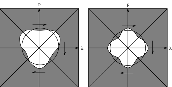
Figure 9.1: $J=3/2$ and $J=2$ special tachyons.

9.3 Correlation Functions from $W_{\infty}$

In this section we will calculate correlation functions involving the operators $W_{\infty}$ as defined in the previous section. The $W_{\infty}$ symmetries will help us organize the Ward identities. As an example, let us start with the two point function. Using

$$<PP>=-\frac{1}{\pi}{\rm Im}\sum_{n=0}^{\infty}\frac{1}{E_{n}-t_{0}}$$ (9.8)

and simple perturbation theory we get

$$<W_{1}W_{2}P>=-\frac{1}{\pi}{\rm Im}\sum_{timeord}\sum_{n,k}\frac{<n\mid W_{1}\mid k><k\mid W_{2}\mid n>}{E_{n}-t_{0}}\frac{1}{ip_{1}+E_{k}-E_{n}}.$$ (9.9)

Since the $W$’s are of the form (9.5), continued to Euclidean time, they are simply raising or lowering operators in the continued harmonic oscillator. This means that only a few of the matrix elements are nonzero. Since $W$ raises by $2m=r-s$ we get

$$<W_{1}W_{2}P>=-\frac{1}{\pi}{\rm Im}\sum_{n}\frac{<n\mid[W_{1},W_{2}]\mid n>}{E_{n}-t_{0}}\frac{1}{i(p_{1}-2m_{1})}.$$ (9.10)

We have reduced the two point function to a one point function using the commutation relations. If we restrict ourselves to the sphere, use the algebra given by (9.2) and directly calculate the one point function we get

$$<W_{1}W_{2}>=-\frac{4(m_{2}J_{1}-m_{1}J_{2})}{p_{1}-2m_{1}}\frac{1}{\pi}\frac{\mu^{J_{1}+J_{2}}}{J_{1}+J_{2}}\mid\log\mu\mid 2^{J_{1}+J_{2}-1}$$ (9.11)

or equivalently

$$<W_{1}W_{2}>=\frac{-2m_{1}}{2m_{1}-p_{1}}\frac{1}{\pi}(2\mu)^{J_{1}+J_{2}}\mid\log\mu\mid.$$ (9.12)

The simplest way to obtain the one point function on the sphere is to use the classical Fermi liquid picture introduced by Polchinski [67]. As we saw in chapter three, we simply need to do the phase space integral

$$<W>=\int dpd\lambda W(p,\lambda).$$ (9.13)

This was also discussed in [19]. To make everything well defined, we need to introduce an extra puncture, i.e. take a derivative with respect to the cosmological constant. Doing that, the integral over the whole Fermi sea becomes just an integral over the Fermi surface

$$<WP>=\oint W(p,\lambda).$$ (9.14)

The integral is to be performed along a hyperbola $\frac{\lambda^{2}-p^{2}}{2}=\mu$. Although the answer is really infinite, we know that the piece nonanalytic in $\mu$ is $\frac{1}{\pi}\mid\log\mu\mid$ for $<PP>$, i.e. when we only integrate $1$. The other zero momentum operators simply involve integrations of $(\frac{\lambda^{2}-p^{2}}{2})^{n}=\mu^{n}$, again constants along the Fermi surface hyperbola, so we get

$$<W^{n,n}P>=-\frac{1}{\pi}(2\mu)^{n}\mid\log\mu\mid$$ (9.15)

and from this (9.11) follows. Our conventions are such that $\alpha^{\prime}=1$. Another approach, which is convenient when calculating correlation functions of nonzero momentum, is to continue to the right side up oscillator where the Fermi surface is a circle. In that case, however, we need to remember to put the Liouville volume $\mid\log\mu\mid$ in by hand. Parenthetically we may note how a general correlation function may be obtained in this way. For instance, the two point function is obtained by perturbing the Hamiltonian, and hence the Fermi surface by one of the operators. If we integrate the other operator against the change in Fermi surface we get the correlation.

Let us now consider the more complicated case of a three point function. In this case there are six different time orderings. Again perturbation theory gives us

$$\frac{1}{\pi}{\rm Im}\sum_{timeord}\sum_{n,m,k}\frac{<n\mid W_{1}\mid m><m\mid W_{2}\mid k><k\mid W_{3}\mid n>}{E_{n}-t_{0}}$$

$$\times\frac{1}{ip_{1}+E_{m}-E_{n}}\frac{1}{ip_{3}+E_{n}-E_{k}}.$$ (9.16)

Let us make the sum over time orderings more explicit. We find three terms of the form

$$\frac{1}{\pi}{\rm Im}\sum_{n}\{\frac{<n\mid(W_{1}W_{2}W_{3}+W_{3}W_{2}W_{1})\mid n>}{E_{n}-t_{0}}\frac{1}{i(p_{1}-2m_{1})i(p_{3}-2m_{3})}+perm\}.$$ (9.17)

This may, after some straightforward manipulations, be rewritten as

$$<W_{1}W_{2}W_{3}>=\frac{<[W_{1},[W_{2},W_{3}]]>}{(p_{1}-2m_{1})(p_{3}+2m_{1}+2m_{2})}+\frac{<[W_{2},[W_{1},W_{3}]]>}{(p_{2}-2m_{2})(p_{3}+2m_{1}+2m_{2})}.$$ (9.18)

For the sphere, we now use the algebra (9.6) and the explicitly calculated one point function to get

$$<W_{1}W_{2}W_{3}>=$$

$$-\frac{(p_{1}-2m_{1})m_{2}m_{3}J_{1}+(p_{2}-2m_{2})m_{1}m_{3}J_{2}+(p_{3}-2m_{3})m_{1}m_{2}J_{3}}{(p_{1}-2m_{1})(p_{2}-2m_{2})(p_{3}-2m_{3})}$$

$$\times\frac{8}{\pi}(2\mu)^{\sum_{n}^{N}J_{n}-1}\mid\log\mu\mid.$$ (9.19)

The general higher point function can be obtained recursively from the three point by use of (9.2) and (9.3). To get the $N$ point function with an additional operator $W_{N}$, we vary the $N-1$ point function with $W_{N}$ knowing that the total variation is zero. The variation consists of two terms. One from varying the action as given by (9.3) and a sum of terms from varying the other operators as given by (9.6). Each of the terms in this sum is obtained by shifting $p_{i}\rightarrow p_{i}+p_{N}$, $m_{i}\rightarrow m_{i}+m_{N}$ and $J_{i}\rightarrow J_{i}+J_{N+1}-1$. We also need to multiply with the Clebsch-Gordan coefficient $2(J_{i}m_{N}-J_{N}m_{i})$. It is an easy exercise to check that (25) is obtained by applying this procedure to (9.11) or (9.12).

There is one subtlety in the variational procedure which should be noted. Previously we derived recursion relations for zero momentum correlation functions by varying $<P>$. Recursion relations for $<PP>$ are obtained from these just by taking a $t_{0}$ derivative. Since the $<P>$ recursion relations involve an explicit $t_{0}$ we find an extra term, $2k<O_{k-1}P>$, in the $<PP>$ recursion relations compared to naïve expectations. The reason is that we insisted on rewriting any conjugated momentum $p$ in terms of $\lambda$’s. The relation involves the potential $U$ and hence depends on the coupling constants, in particular $t_{0}$. The statement is that although $<U(\lambda)P>=<\frac{p^{2}}{2}P>$, we have in fact $<U(\lambda)PP>\neq<\frac{p^{2}}{2}PP>$. In the $W_{\infty}$ recursion relations we are discussing, we never perform any evaluations like this and hence need not to worry about these issues. For instance, if we want to include extra punctures in the correlation functions we are free to do so without extra terms in the $W_{\infty}$ relations.

Using this method one can write down several different recursion relations. One simple example is:

$$<T_{J,J}W_{J_{1},m_{1}}\prod_{i=2}^{N}T_{J_{i},J_{i}}>=\frac{4J(m_{1}-J_{1})}{p-2J}<W_{J+J_{1}-1,J+m_{1}}\prod_{i=2}^{N}T_{J_{i},J_{i}}>.$$ (9.20)

We will come back to this relation later, when we compare with the Liouville model results.

Rather than considering these general expressions, let us look at a couple of important examples where the form of the general $N$ point function is particularly simple.

The first example is the $N$ point function of special tachyons. It is given by

$$<\prod_{n=1}^{N}T_{n}>=\frac{-\prod_{n=1}^{N}2J_{n}}{\prod_{n=2}^{N}(2J_{n}-p_{n})}\frac{2}{\pi}\frac{d^{N-3}}{d\mu^{N-3}}(2\mu)^{\sum_{n=1}^{N}J_{n}-1}\mid\log\mu\mid.$$ (9.21)

The quantum numbers have been chosen as $m_{n}=J_{n}$ for $n>1$ and $m_{1}=-J_{1}$. This is just the pole part of the general tachyon correlation function as computed both in the matrix model [36, 58] and in the Liouville theory [36, 24], up to a factorized normalization factor. The proof is by varying the three point. We cannot just vary the three point tachyon correlation function, since some of the $J$’s are really $m$’s in disguise and $J$ and $m$ vary differently. Instead we start with the general three point and make an arbitrary number of tachyon variations. A simplification is that we at each step only have to vary the single negative chirality tachyon. It is only from there we will get a nonzero Clebsch-Gordan coefficient. Following the prescription above, performing $N-3$ variations we get

$$<\prod_{n=1}^{N}T_{n}>=-\left[(p_{1}-2m_{1}+\sum_{i=4}^{N}(p_{i}-2m_{i}))m_{2}m_{3}(J_{1}+\sum_{i=4}^{N}J_{i}-N+3)\right.$$

$$\left.+(p_{2}-2m_{2})(m_{1}+\sum_{i=4}^{N}m_{i})m_{3}J_{2}+(p_{3}-2m_{3})(m_{1}+\sum_{i=4}^{N}m_{i})m_{2}J_{3}\right]$$

$$\times\frac{\prod_{i=4}^{N}4(J_{i}(m_{1}+\sum_{j=i+1}^{N}m_{j})-(J_{1}+\sum_{j=i+1}^{N}J_{j}-N+i)m_{i})}{(p_{1}-2m_{1}+\sum_{i=4}^{N}(p_{i}-2m_{i}))\prod_{n=2}^{N}(p_{n}-2m_{n})}$$

$$\times\frac{8}{\pi}(2\mu)^{\sum_{n=1}^{N}J_{n}-N+2}\mid\log\mu\mid.$$ (9.22)

The product in the denominator is the product of all the Clebsch-Gordan coefficients of the variations. Note that each get shifted by the successive variations. By the use of momentum conservation and evaluating the $m$’s as $J$’s, the formula (9.21) is proved. This derivation shows how the combinatorial factor from the $\mu$ derivatives is a consequence of the $W_{\infty}$ symmetry.

Since this derivation is quite illuminating, it might be reasonable to consider a particular example which is more transparent than the general derivation above. Let us consider a four point tachyon correlation function. A sketch of the relevant setup with three vertices and a one point is given in figure 9.2. The vertices give rise to the factor

$$(J_{2}m_{1}-J_{1}m_{2})(J_{3}(m_{1}+m_{2})-(J_{1}+J_{2}-1)m_{3})$$

$$\times(J_{4}(m_{1}+m_{2}+m_{3})-(J_{1}+J_{2}+J_{3}-2)m_{4})$$

$$=2J_{1}J_{2}J_{3}J_{4}(J_{1}+J_{2}+J_{3}+J_{4}-1)(J_{1}+J_{2}+J_{3}+J_{4}-2).$$ (9.23)

The last factor is then cancelled by the one point function. The remainder, apart from a factorized part, is the well known $\sum J_{i}-1$ found by many other methods.

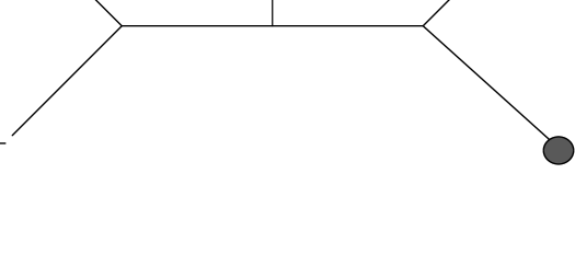
Figure 9.2: Graph for four point tachyon correlation function.

If we want to consider the zero momentum operators, we have to be careful. The Clebsch-Gordan coefficients are zero in this case but these zeroes precisely cancel the momentum poles and leave a finite result. We get

$$<\prod_{n=1}^{N}W_{n}>=-\frac{1}{\pi}\frac{d^{N-2}}{d\mu^{N-2}}(2\mu)^{\sum_{n=1}^{N}J_{n}}\mid\log\mu\mid.$$ (9.24)

We will use induction for the proof. We find

$$<\prod_{n=1}^{N+1}W_{n}>=-\sum_{k}4(J_{N+1}m_{k}-J_{k}m_{N+1})\frac{1}{p_{N+1}-2m_{N+1}}$$

$$\times\frac{1}{\pi}\frac{d^{N-2}}{d\mu^{N-2}}(2\mu)^{\sum_{n=1}^{N+1}J_{n}-1}\mid\log\mu\mid.$$ (9.25)

If we then put $p_{N+1}=0$ and use that the sum of all $m$’s must be zero the result follows. This can also be checked by an explicit phase space calculation.

9.4 Some Consistency Checks

Let us now study the results of the previous section more closely. In particular we will compare the two point correlation functions with the results derived in the last chapter. These were correlation functions of pure powers of the matrix eigenvalue, without any momentum powers. In terms of the W’s they are given by

$$O_{n}=\sum_{k=0}^{n}\left(\begin{array}[]{c}n\\ k\end{array}\right)W^{n,k-n}\frac{1}{2^{n}}.$$ (9.26)

From this follows that the two point function is given by

$$<O_{n}O_{m}>_{q}=\frac{1}{2^{n+m}}\sum_{k=0}^{n}\sum_{l=0}^{m}\left(\begin{array}[]{c}n\\ k\end{array}\right)\left(\begin{array}[]{c}m\\ l\end{array}\right)<W^{n-k,k}_{q}W^{m-l,l}_{-q}>.$$ (9.27)

Using (9.12) and some simple algebra we find

$$\frac{-1}{2^{\frac{1}{2}(n+m)}}\frac{1}{\pi}\mu^{\frac{1}{2}(n+m)}\mid\log\mu\mid\sum_{k=0}^{n}\left(\begin{array}[]{c}n\\ k\end{array}\right)\left(\begin{array}[]{c}m\\ \frac{n+m}{2}-k\end{array}\right)\frac{4(\frac{n}{2}-k)^{2}}{4(\frac{n}{2}-k)^{2}-q^{2}}.$$ (9.28)

In precise agreement with [15] and the result (8.25) of the previous chapter, recalling our convention $\alpha^{\prime}=1$. We can now understand why the $O$ operators gave correlation functions with sets of poles and were, depending on momentum, capable of exciting several special states [15]. They were, in fact, linear combinations of all special operators of a given gravitational dimension i.e. spin $J$. The above construction with the generators (9.1) of the $W_{\infty}$ disentangles the correlation functions. This means that the matrix model operators to be identified with the Liouville model special states are those defined in (9.5).

Let us briefly comment on the meaning of the momentum poles. As emphasized in [49] we should not treat the poles and the $\mid\log\mu\mid$ in the correlation functions asymmetrically since the source of the $\mid\log\mu\mid$ is also a momentum pole. In fact, all the poles should be thought of as cut off by $\mid\log\mu\mid$. A general $N$ point function (without zero momentum operators) would then have $\mid\log\mu\mid^{N}$. This proliferation of logarithms was also noted in [24].

Let us make some further tests of the correlation functions in (9.12) and (9.19). This will illustrate some very simple consequences of the $W_{\infty}$ algebra. In fact, the seemingly innocent representation of the puncture and the dilaton as $\mu$ and $t_{2}$ derivatives respectively is a reflection of the $W_{\infty}$. Let us give a formal argument for this. First the puncture. Write the $SU(2)$ quantum numbers of the puncture as $J$ and $m$, which both will be taken to zero. Choose one of the operators in (9.19) to be a puncture. We get

$$<W_{1}W_{2}P>=-(J_{1}+J_{2})\frac{2m_{1}}{2m_{1}-p_{1}}\frac{2}{\pi}(2\mu)^{J_{1}+J_{2}-1}\mid\log\mu\mid,$$ (9.29)

which, by comparing with the two point function (9.11), shows how the puncture is represented as a $\mu$ derivative. The case of the dilaton is equally simple. Proceeding as above we find

$$<W_{1}W_{2}D>=-\left[(J_{1}+J_{2})\frac{2m_{1}}{2m_{1}-p_{1}}+\frac{4m_{1}^{2}}{(2m_{1}-p_{1})^{2}}\right]\frac{2}{\pi}(2\mu)^{J_{1}+J_{2}}\mid\log\mu\mid.$$ (9.30)

If we introduce explicit $t_{2}$’s in the two point function we can write it as

$$<W_{1}W_{2}>=\frac{-2m_{1}}{2m_{1}-p_{1}/(-2t_{2})^{1/2}}\frac{1}{\pi}\frac{1}{(-2t_{2})^{1/2}}\left(\frac{2\mu}{(-2t_{2})^{1/2}}\right)^{J_{1}+J_{2}}\mid\log\mu\mid.$$ (9.31)

Taking a $(-2t_{2})^{1/2}$ derivative, we arrive at

$$<W_{1}W_{2}D>=-\left[(J_{1}+J_{2}+1)\frac{2m_{1}}{2m_{1}-p_{1}}+\frac{2m_{1}p_{1}}{(2m_{1}-p_{1})^{2}}\right]\frac{2}{\pi}(2\mu)^{J_{1}+J_{2}}\mid\log\mu\mid,$$ (9.32)

which indeed reproduces (9.30). We must now return to the issue of how precisely the dilaton is defined. Recall the original matrix model action

$$\beta\int dt[p\dot{\lambda}-\frac{1}{2}p^{2}-t_{2}\lambda^{2}]$$ (9.33)

with $\beta$ dimensionless, $t_{2}$ having the dimension of energy squared, and $p^{2}$ and $\lambda^{2}$ the dimensions of energy and one over energy respectively. To obtain (9.31) as a generating functional for dilaton insertions with the above definition of the dilaton we should rescale $\lambda$ and $p$ to make them dimensionless. We find

$$\beta\int dt[p\dot{\lambda}-\frac{1}{\sqrt{2}}(-t_{2})^{1/2}(p^{2}-\lambda^{2})].$$ (9.34)

Hence the matrix model dilaton should be represented by $(-2t_{2})^{1/2}$ derivatives. This is the rescaling eluded to in chapter seven, in the context of the Wheeler de Witt equation.

Let us give some further illustrations in the case of puncture and dilaton insertions from the field theoretic point of view. We begin with the puncture. Starting with a general correlation function and inserting a puncture does not change the Veneziano-like integral which has to be calculated. When we insert a puncture, we also must remove one of the screening insertions. The only thing which changes is the zero mode part of the calculation. We recall the result

$$\int d\phi e^{m\phi-\Delta e^{-\phi}}\sim\Gamma(-m)\Delta^{m}.$$ (9.35)

If we start with $\Gamma(-m)\mu^{m}$ we end up with $\Gamma(-m+1)\mu^{m-1}=-m\Gamma(-m)\mu^{m-1}$ when we remove a screening insertion. Comparing with (9.29) this shows the origin of the $W_{\infty}$ related factor in the tachyon correlation function. It is a consequence of the changing number of puncture screening operators needed.

For the tachyons the issue of connected or 1PI amplitudes is trivial for our case with just one tachyon of differing chirality. There can not be any internal punctures just from kinematics. This is no longer the case when we turn to the dilaton. The crucial point is that the dilaton can be represented as a $t_{2}$ derivative. Usually, this is precisely equivalent to using the ordinary free field contractions, giving Veneziano-like correlation functions. Inserting a dilaton in some tachyon correlation function means taking derivatives with respect to $t_{2}$ (i.e. $1/\alpha^{\prime}$). For dimensional reasons, all tachyon momenta are accompanied by a $t_{2}$. Without explicit $t_{2}$’s one could write $k\frac{\partial}{\partial k}$ for the dilaton. For a dilaton insertion in a nonzero momentum correlation function, the dominating pole contribution comes from letting the $t_{2}$ derivative act directly on the poles. All other terms are clearly less singular. This gives the second term in (9.32). At zero momentum we must also consider the dependence from the $t_{2}$’s which go together with the $\mu$’s. The latter is a consequence of dealing with 1PI rather than connected correlation functions. One could in fact obtain the result by considering the explicit combinations of 1PI amplitudes into connected ones. To be more precise, if we want to obtain the 1PI amplitude from the connected amplitude, we must amputate external puncture legs but also subtract of the diagrams with internal puncture propagators. In particular, we need to subtract a diagram where a puncture goes off and converts into a dilaton. This diagram, therefore, involves a puncture insertion and gives a contribution corresponding to a $\mu$ derivative. The procedure is illustrated in figure 9.3. This is then simulated by an explicit $t_{2}$ accompanying the $\mu$’s to assure the proper subtraction, which corresponds to the first term in (9.32) and only becomes relevant compared to the second term at zero momentum. Otherwise we will get one power less of $\mid\log\mu\mid$’s. We need not restrict ourselves to a dilaton among special tachyons. The same reasoning works for a dilaton inserted in a general correlation function.

Figure 9.3: Relation between dilaton 1PI and connected correlation functions.

From these two examples we can conclude that the 1PI nature of the correlation functions is very important in the case of zero momentum.

Finally, it is useful to think of the correlation functions from a group theoretic point of view. The symmetry can be used to determine all correlation functions given the special tachyon correlation functions which may be computed by other means. The reason is that all $J$ and $m$ dependence of any correlation function is given by some combination of Clebsch-Gordan coefficients. For given $J$’s we need the Clebsch-Gordan coefficients of $SU(2)$, the $3j$ symbols, to get the $m$ dependence. To be more explicit let us however look at an example, the three point function, to see how the invariance properties determine the correlation functions.

The three point function is obtained by considering coupling $(J_{1},m_{1})$, $(J_{2},m_{2})$ and $(J_{3},m_{3})$ (with $m_{1}+m_{2}+m_{3}=0$) to $(J_{1}+J_{2}+J_{3}-2,0)$. A complication is that there are in general several different channels to sum over. This is true already for the three point function. The reason, as we have seen, is that we actually should think of the three point function as a four point function. The fourth leg carries the excess Liouville momentum, i.e. $J$ quantum number, into the vacuum. This is a consequence of the nonconservation of Liouville momentum. Let us use the tachyon three point function for normalization. It is given by

$$<T_{1}T_{2}T_{3}>=\frac{-8J_{1}J_{2}J_{3}}{(2m_{2}-p_{2})(2m_{3}-p_{3})}\frac{2}{\pi}(2\mu)^{J_{1}+J_{2}+J_{3}-1}\mid\log\mu\mid,$$ (9.36)

where we have kept the normalization choice of (9.21). Tachyons 2 and 3 are of positive chirality, while tachyon 1 has negative chirality. There are two possible channels corresponding to either $p_{2}=2m_{2}$ or $p_{3}=2m_{3}$, i.e. 1 and 2 coming together or 1 and 3 coming together. The group theoretic factor in each case is simply proportional to a product of $3j$ symbols. One for each vertex. For the 1-2 channel the factor is

$$\left(\begin{array}[]{c}J_{1}J_{2}J\\ m_{1}m_{2}m_{3}\end{array}\right)\left(\begin{array}[]{c}JJ_{3}J^{\prime}\\ -m_{3}m_{3}0\end{array}\right),$$ (9.37)

where $J=J_{1}+J_{2}-1$ and $J^{\prime}=J_{1}+J_{2}+J_{3}-2$. Just retaining the $m$ dependence and adding the two channels we find

$$(2m_{2}-p_{2})(J_{1}m_{2}-J_{2}m_{1})m_{3}+(2m_{3}-p_{3})(J_{1}m_{3}-J_{3}m_{1})m_{2}$$

$$=-(2m_{1}-p_{1})J_{1}m_{2}m_{3}-(2m_{2}-p_{2})J_{2}m_{1}m_{3}-(2m_{3}-p_{3})J_{3}m_{1}m_{2}$$ (9.38)

which agrees with (25) after using (9.36) to fix the normalization and $J$ dependence. This should come as no surprise since we have just rephrased the previous calculation slightly.

Another convenient way to obtain more general correlation functions is through factorization. This is actually already implicit in our previous calculations. In fact, if we look at (9.22), we see the complete factorization of the tachyon correlation function into a product of three point functions, each given by a $3j$ symbol times a single zero momentum one point function. This last piece represents the extra leg in any correlation function which absorbs excess Liouville momenta. One may note that these three point functions in fact involve states of the wrong dressing. This was also pointed out in [71]. Strictly speaking, the expression in (9.22) is just for one channel, the one where 1 fuses with 2 then with 3 etc. All channels,however, give identical contributions and can not be distinguished. Clearly, the tachyon correlation function is consistent with the single $W_{\infty}$ factorization result.

9.5 Summary

In this chapter we have exploited the matrix model $W_{\infty}$ algebra to derive correlation functions. The methods we have used provide a substantial simplification compared to previous calculations. Also, the correct association of special states and $W_{\infty}$ elements disentangles the correlation functions in a neat way.

So far we have just looked at the sphere. In the next chapter we will see how the picture generalizes to higher genus.

Chapter 10 Higher Genus Correlation Functions

10.1 Introduction

In the previous chapter we showed how to use the $W_{\infty}$ algebra of the $c=1$ matrix model to derive correlation functions of special states. In particular, the method is applicable to the special tachyons. In this chapter we will treat the higher genus case more explicitly. The motivation is that by deriving the results using the $W_{\infty}$, rather than just brute force calculations, the crucial physics will be more apparent. Hopefully one can in this way obtain useful guidelines for constructing a field theory approach to higher genus. In [18], similar results as in the previous chapter were obtained independently. The authors combine the $W_{\infty}$ properties of the system with the powerful path integral methods of [58] to calculate correlation functions. This is an useful approach for studying the matrix model. We feel however, that the approach advocated in previous chapters and used in this chapter, will prove very useful for field theory purposes. Furthermore, there are certain subtle issues like ordering in the matrix model definition of the special states which can not be addressed in the path integral approach.

An important feature of the matrix model higher genus calculations is a deformation of the classical, genus zero $W_{\infty}$ algebra with Planck’s constant, i.e. the genus coupling, as parameter. This is simply a result of replacing the Poisson brackets with commutators.

As mentioned above, at higher genus we must also face the problem of ordering when we define the special state operators. For the special tachyons there is no ambiguities, but for the general special state there are. However, in the very explicit calculations we will be doing, the question of ordering will be important even in the case of tachyons. Not for the final results, but for the intermediate steps. We will choose Weyl ordering. Weyl ordering means that one takes an average over all possible orderings with equal weights. The reasons for this choice are several. It is from many points of view the most “natural” ordering prescription. In a path integral approach it would be the automatic choice. This is of course connected with another reason, that there exist simple formulas for calculations involving Weyl ordering. An important question is of course whether this is the ordering prescription which will be relevant in the comparison with field theory. It is conceivable that there will not exist an unique choice but rather that we have to live with this ambiguity which, after all, only amounts to a linear transformation.

10.2 The Algebra

We begin our discussion by considering the $W_{\infty}$ algebra of the $c=1$ matrix model. Our conventions throughout this chapter are such that $\alpha^{\prime}=1$. As explained in the previous chapter, the theory is organized by a $W_{\infty}$ algebra generated by the matrix eigenvalue and its conjugate momentum. Classically, it is given through the Poisson brackets by

$$\{W_{J_{1},m_{1}},W_{J_{2},m_{2}}\}=4i(m_{2}J_{1}-m_{1}J_{2})W_{J_{1}+J_{2}-1,m_{1}+m_{2}}$$ (10.1)

where

$$W_{J,m}=(\lambda-ip)^{J+m}(\lambda+ip)^{J-m}=2^{J}a^{\dagger J+m}a^{J-m}.$$ (10.2)

For convenience, we have introduced the step up and down operators $a^{\dagger}$ and $a$. As shown in the previous chapter this algebra may be used to organize the special state correlation functions in the theory. Parallel work has revealed a similar structure in the field theory [50], although the precise connection between the two approaches is not yet clear. The great advantage of the matrix model is of course that we may extend the calculation to arbitrary genus. The main new ingredient at higher genus is the deformation of the algebra mentioned in the introduction. At higher genus, i.e. quantum mechanically, we must also be careful and choose an ordering prescription. As explained above we choose Weyl ordering where the new algebra is simply given by the Moyal brackets

$$\frac{1}{i\hbar}[W_{1},W_{2}]=\{W_{1},W_{2}\}_{M}=\frac{2}{\hbar}\sin\frac{\hbar}{2}(\frac{\partial}{\partial p_{2}}\frac{\partial}{\partial\lambda_{1}}-\frac{\partial}{\partial p_{1}}\frac{\partial}{\partial\lambda_{2}})W_{1}W_{2}$$ (10.3)

which allow for simple calculations. The proof is elementary, but we provide it for completeness.

A Weyl ordered operator can be written as

$$\hat{A}(\hat{p},\hat{q})_{W}=\frac{1}{(2\pi)^{2}}\int A(p,q)e^{-i(\tau p+\theta q)}e^{i(\tau\hat{p}+\theta\hat{q})}dpdqd\tau d\theta.$$ (10.4)

If we take the commutator of two such Weyl ordered operators, $\hat{A}_{W}$ and $\hat{B}_{W}$, we encounter the expression

$$[e^{i(\tau_{1}\hat{p}+\theta_{1}\hat{q})},e^{i(\tau_{2}\hat{p}+\theta_{2}\hat{q})}]=2i\sin\frac{\hbar}{2}(\tau_{1}\theta_{2}-\tau_{2}\theta_{1})e^{i(\tau_{1}+\tau_{2})\hat{p}+i(\theta_{1}+\theta_{2})\hat{q})}.$$ (10.5)

The $\sin$ is then rewritten as $2i\sin\frac{\hbar}{2}(\frac{\partial}{\partial p_{2}}\frac{\partial}{\partial\lambda_{1}}-\frac{\partial}{\partial p_{1}}\frac{\partial}{\partial\lambda_{2}})$ by partial integration. The $\tau_{1}-\tau_{2}$ and $\theta_{1}-\theta_{2}$ integrations give $\delta$ functions which fixes $p_{1}=p_{2}$ and $q_{1}=q_{2}$ respectively. From this the result follows.

An equivalent way of exhibiting the quantum deformation is to focus on (10.5), which in fact is a very old result, [62], and inspired by this introduce a generalized loop operator [19]. Instead of (8.6) we define

$$w(k,l)=e^{kp+l\lambda},$$ (10.6)

where $p$ and $\lambda$ are the conjugate variables. We then have

$$[w(k_{1},l_{1}),w(k_{2},l_{2})]=2i\sin\frac{\hbar}{2}(k_{1}l_{2}-l_{1}k_{1})w(k_{1}+k_{2},l_{1}+l_{2})$$ (10.7)

with $\hbar\rightarrow 0$ giving back a $W_{\infty}$. Interestingly, it can be shown [4] that (10.7) is a representation of $SU(N)$ with $\hbar=1/N$. This is reminiscent of the original unitary symmetry of the matrix model.

Let us give a simple example of a higher genus commutator. Using the Moyal bracket it immediately follows that, for $\hbar=1$,

$$[a^{m},a^{\dagger n}]=\sum_{g=0}^{\infty}\frac{1}{2^{2g}(2g+1)!}\prod_{k=0}^{2g}(m-k)(n-k)(a^{m-2g-1}a^{\dagger n-2g-1})_{W}.$$ (10.8)

The continuation to the upside down harmonic oscillator gives an extra factor of $i$ and an extra $(-1)^{g}$. This result will be extensively used in a later section where we calculate tachyon N-point functions.

For clarity, let us calculate explicitly a two point function to all genus. We choose the correlator between spin $J=3/2$, $m=1/2$ and $J=3/2$, $m=-1/2$. To do that we need to calculate $<W_{2,0}P>$. This is easy. We have

$$<W_{2,0}P>=-\frac{1}{\pi}{\rm Im}\sum_{n=0}^{\infty}\frac{(2E_{n})^{2}-1}{E_{n}-t_{0}}.$$ (10.9)

The extra term $-1$ comes from Weyl ordering and will be thoroughly discussed in the next section. If we keep only terms nonanalytic in $t_{0}$ this reduces to

$$<W_{2,0}P>=(4t_{0}^{2}-1)<PP>.$$ (10.10)

To evaluate our two point we use the Moyal bracket continued to the upside down harmonic oscillator to calculate

$$[W_{3/2,1/2},W_{3/2,-1/2}]=i(6W_{2,0}+4W_{0,0})$$ (10.11)

(9.10) and (10.10) then finally give

$$<W_{3/2,1/2}W_{3/2,-1/2}P>=(24t_{0}^{2}-2)<PP>\frac{1}{1-p}.$$ (10.12)

The same procedure may be used to calculate arbitrary correlation functions.

In the previous chapter, it was shown how to calculate special state correlation functions using this algebra. The number of operators in the correlation functions are reduced one by one using the algebra. The last step, however, involves the calculation of a remaining zero momentum one point function. This is where the cosmological screening charges sit. Let us therefore turn to the issue of calculating such objects.

10.3 The One Point Functions

To obtain the zero momentum special state one point functions at higher genus, we need to be careful. From the algebra we understand that they are given in terms of $(H^{n})_{W}$. These are just powers of the Hamiltonian. But it is important to remember the Weyl ordering. This will make the one point functions quite complicated. We need to rewrite the Weyl ordered powers in terms of something simpler. The objects with simple correlation functions are clearly the $H^{n}$, which give

$$t^{n}_{0}<PP>$$ (10.13)

since the resulting $E_{m}^{n}$ in the trace can be replaced by $t_{0}^{n}$ up to terms analytic in $t_{0}$. To obtain the $(H^{n})_{W}$ one point functions we therefore need to perform the Weyl ordering and express the result as a polynomial in $H$. One way to do this is to use the standard formula

$$(a^{m}a^{\dagger n})_{W}=2^{-m}\sum_{l=0}^{m}\left(\begin{array}[]{c}n\\ l\end{array}\right)a^{\dagger m-l}a^{n}a^{\dagger l}.$$ (10.14)

See e.g. [54]. If we put $m=n$ and take the expectation value in the eigenstate $r$ we get

$$2^{-n}\sum_{l=0}^{n}\left(\begin{array}[]{c}n\\ l\end{array}\right)\prod_{k=0}^{n-1}(r+l-k),$$ (10.15)

and finally

$$(H^{n})_{W}=2^{-n}\sum_{l=0}^{n}\left(\begin{array}[]{c}n\\ l\end{array}\right)\prod_{k=0}^{n-1}(H-\frac{1}{2}+l-k).$$ (10.16)

This is unfortunately a very complicated polynomial. In the next section we will explicitly calculate some tachyon correlation functions. To do so we need explicit expression for the coefficients in (10.16). By some tedious algebra, which is greatly simplified if Mathematica is used, the following expression can be obtained

$$\begin{array}[]{l}(H^{n})_{W}=H^{n}+\frac{1}{24}(2n-1)n(n-1)H^{n-2}\\ \\ +\frac{1}{5760}(20n^{2}-48n+7)\prod_{k=0}^{3}(n-k)H^{n-4}\\ \\ +\frac{1}{2903040}(280n^{3}-1596n^{2}+1874n-93)\prod_{k=0}^{5}(n-k)H^{n-6}+...\end{array}$$ (10.17)

The continued case is obtained by sending $H^{n-2k}\rightarrow(-1)^{k}H^{n-2k}$. This is enough up to genus 3 for the general correlation function. In appendix 10A, the expansion is shown up to genus 7. These expressions are really remarkably complicated, and responsible for the complicated structure of the higher genus correlation functions. The piece coming from the $W_{\infty}$ algebra is much simpler.

For clarity, let us give an example. We choose $J=4$. We find

$$\frac{1}{16}<W_{4,0}P>=<H^{4}P>-\frac{7}{2}<H^{2}P>+\frac{9}{16}<PP>$$

$$=-\frac{1}{\pi}(t_{0}^{4}-\frac{7}{2}t_{0}^{2}+\frac{9}{16})\log\mu+O(1/t_{0}^{2}).$$ (10.18)

where we note resonance contributions up to genus 2, but no higher. The same general structure is clearly found for the tachyon correlation functions. Poles are present only up to some genus. The precise value depends on the scaling (i.e. momentum).

10.4 Tachyon Correlation Functions

We now need to combine these results with those given by the deformed $W_{\infty}$ algebra to get the tachyon correlation functions. This is, in principle, rather simple. In fact, one can write down a set of diagrammatic rules which give the correlation functions.

By the variational procedure introduced in the last chapter one can show that in the case of $(N-1,1)$ amplitudes it is possible to arrange things in such a way that only one basic graph is needed. There exist other choices too, involving sums over several graphs, but this one is clearly the simplest. The graph, shown in figure 9.2, has a $T^{-}$ at one end and the necessary one point function at the other. In between are the $T^{+}$ distributed in some order. The order does not matter, but we should pick just one ordering, no sum. To see this, one can start with the two point function of a $T^{+}$ and a $T^{-}$. All subsequent $T^{+}$ variations will only give a nonzero value when they hit the $-$ leg. If we are considering a genus $g$ correlation function, we must partition the handles in all possible ways among the vertices and the one point function. Each such diagram is then given a certain factor according to the following rules.

For each vertex write down a factor $f_{g_{k}}(p_{k})$ given by

$$f_{g_{k}}(p_{k})=\frac{(-1)^{g_{k}}}{2^{2g_{k}}(2g_{k}+1)!}(p_{k}-1)(p_{k}-2)...(p_{k}-2g_{k}),$$ (10.19)

where $p_{k}$ is the momentum of the $k$’th (positive) tachyon and $g_{k}$ the genus of the corresponding vertex. This is obtained from (10.8). Strictly speaking the formulae are only valid when $p=2J$, i.e. for special tachyons. The one point function is given a factor $h_{\tilde{g}}$ according to

$$\begin{array}[]{l}h_{0}(p)=1\\ h_{1}(p)=\frac{-1}{24}(2p-1)\\ h_{2}(p)=\frac{1}{5760}(20p^{2}-48p+7)\\ h_{3}(p)=\frac{-1}{2903040}(280p^{3}-1596p^{2}+1874p-93),\end{array}$$ (10.20)

where the argument $p$ is

$$\frac{1}{2}\sum_{k=1}^{N}\mid p_{k}\mid-N+2(\tilde{g}-g)+1=\mid p_{1}\mid-N+2(\tilde{g}-g)+1.$$ (10.21)

$\tilde{g}$ is the genus associated with the one point function. Clearly, $\sum_{k=2}^{N}g_{k}+\tilde{g}=g$. Some additional $h_{\tilde{g}}$ polynomials may be read off from appendix 10A while the general case is generated by (10.16). In both (10.19) and (10.20) we have extracted a common factor depending only on the momentum of the single negative chirality tachyon.

Using this technique, the two point function would be calculated as

$$p^{2}f_{0}(p)h_{0}(p-1)\frac{t_{0}^{p-1}}{p-1}+p^{2}(p-1)(p-2)$$

$$\times\left[f_{1}(p)h_{0}(p-3)+f_{0}(p)h_{1}(p-1)\right]\frac{t_{0}^{p-3}}{p-3}+p^{2}(p-1)(p-2)(p-3)(p-4)$$

$$\times\left[f_{2}(p)h_{0}(p-5)+f_{1}(p)h_{1}(p-3)+f_{0}(p)h_{2}(p-1)\right]\frac{t_{0}^{p-5}}{p-5}+...$$ (10.22)

up to genus $2$. In particular, if we concentrate on genus 2 the relevant calculation involves

$$p^{2}(p-1)...(p-4)\left[\frac{1}{1920}(p-1)...(p-4)+\right.$$

$$\left.\frac{1}{576}(p-1)(p-2)(2p-7)+\frac{1}{5760}(20(p-1)^{2}-48(p-1)+7)\right]$$

$$=p^{2}(p-1)...(p-4)\frac{1}{5760}(3p^{4}-10p^{3}-5p^{2}+12p+7).$$ (10.23)

Although the algebra is somewhat tedious, the generalization to higher genus and N-point functions is straightforward. As an example the three point function at genus 3 is computed in appendix 10B. Here, we will simply state the results for N-point functions up to genus $3$.

$$\frac{\partial^{N-3}}{\partial t_{0}^{N-3}}t_{0}^{p_{1}-1}-\frac{1}{24}(\sum_{i=2}^{N}p_{i}^{2}-p_{1}-1)\frac{\partial^{N-1}}{\partial t_{0}^{N-1}}t_{0}^{p_{1}-1}$$

$$+\frac{1}{5760}(3\sum_{i=2}^{N}p_{i}^{4}+10\sum_{i,j=2,i>j}^{N}p_{i}^{2}p_{j}^{2}-10p_{1}\sum_{i=2}^{N}p_{i}^{2}-5(\sum_{i,j=2,i>j}^{N}(p_{i}-p_{j})^{2}-(N-3)\sum_{i=2}^{N}p_{i}^{2})$$

$$+12p_{1}+7)\frac{\partial^{N+1}}{\partial t_{0}^{N+1}}t_{0}^{p_{1}-1}$$

$$-\frac{1}{2903040}(9\sum_{i=2}^{N}p_{i}^{6}+63\sum_{i,j=2,i>j}^{N}p_{i}^{2}p_{j}^{4}+210\sum^{N}_{i,j,l=2,i>j>l}p_{i}^{2}p_{j}^{2}p_{l}^{2}$$

$$-p_{1}(63\sum_{i=2}^{N}p_{i}^{4}+210\sum_{i,j=2,i>j}^{N}p_{i}^{2}p_{j}^{2})+42\sum_{i=2}^{N}p_{i}^{4}+210\sum_{i,j=2,i>j}^{N}p_{i}^{3}p_{j}$$

$$+210\sum^{N}_{i,j,l,i>j}p_{i}p_{j}p_{l}^{2}+p_{1}(217\sum_{i=2}^{N}p_{i}^{2}-70\sum_{i,j=2,i>j}^{N}p_{i}p_{j})-294\sum_{i,j=2,i>j}^{N}p_{i}p_{j}$$

$$-205p_{1}-93)\frac{\partial^{N+3}}{\partial t_{0}^{N+3}}t_{0}^{p_{1}-1}.$$ (10.24)

This is to be multiplied with the appropriate factorized pole factor. The result may be compared to other calculations of the correlation functions. Clearly this is a very complicated expression which practical application is probably very limited. The main point is, however, not this expression in itself, but rather the way in which we have derived it.

10.5 Summary

We have seen how to calculate special tachyon correlation functions in the matrix model using the deformed $W_{\infty}$ algebra. The algebra nicely organizes the correlation functions even at higher genus.

A natural challenge to the field theory approach is to reproduce this deformation of the algebra, which we have described and found to be important for the structure of the correlation functions. One would expect that the deformation is related to contour integrals of the currents which when pulled back over the surface, away from any insertions, fail to yield zero since they get caught up around handles and cannot be contracted to points.

Appendix 10A

Weyl ordering of powers of the Hamiltonian for computations up to genus 7:

$$\begin{array}[]{l}(H^{n})_{W}=H^{n}+\frac{1}{24}(2n-1)n(n-1)H^{n-2}\\ \\ +\frac{1}{5760}(20n^{2}-48n+7)\prod_{k=0}^{3}(n-k)H^{n-4}\\ \\ +\frac{1}{2903040}(280n^{3}-1596n^{2}+1874n-93)\prod_{k=0}^{5}(n-k)H^{n-6}\\ \\ +\frac{1}{1393459200}(2800n^{4}-29120n^{3}+85544n^{2}-68368n+1143)\prod_{k=0}^{7}(n-k)H^{n-8}\\ \\ +\frac{1}{367873228800}(12320n^{5}-203280n^{4}+1100528n^{3}-2255352n^{2}\\ \\ +1422434n-7665)\prod_{k=0}^{9}(n-k)H^{n-10}\\ \\ +\frac{1}{24103053950976000}(11211200n^{6}-269068800n^{5}+2312950640n^{4}-8743967232n^{3}\\ \\ +14194825268n^{2}-7658714592n-12730293)\prod_{k=0}^{11}(n-k)H^{n-12}\\ \\ +\frac{1}{578473294823424000}(3203200n^{7}-105385280n^{6}+1315394080n^{5}-7873930064n^{4}\\ \\ +23465896792n^{3}-32333229596n^{2}+15636417798n-7740495)\prod_{k=0}^{13}(n-k)H^{n-14}+...\end{array}$$

Appendix 10B

In this appendix we calculate the tachyon three point function at genus 3. As explained in the main text we should write down all possible partitions of the three handles among the vertices and the one point. This gives

$$\left[f_{3}(p_{3})f_{0}(p_{2})+f_{0}(p_{3})f_{3}(p_{2})+f_{2}(p_{3})f_{1}(p_{2})+f_{1}(p_{3})f_{2}(p_{2})\right]h_{0}(p_{1}-8)$$

$$+\left[f_{2}(p_{3})f_{0}(p_{2})+f_{0}(p_{3})f_{2}(p_{2})+f_{1}(p_{3})f_{1}(p_{2})\right]h_{1}(p_{1}-6)$$

$$+\left[f_{1}(p_{3})f_{0}(p_{2})+f_{0}(p_{3})f_{1}(p_{2})\right]h_{2}(p_{1}-4)+f_{0}(p_{3})f_{0}(p_{2})h_{3}(p_{1}-2).$$ (10.25)

Using the expressions (10.19) and (10.20) we find

$$\frac{1}{2^{6}7!}\left[(p_{3}-1)...(p_{3}-6)+(p_{2}-1)...(p_{2}-6)\right]$$

$$+\frac{1}{2^{6}5!3!}\left[(p_{3}-1)...(p_{3}-4)(p_{2}-1)(p_{2}-2)+(p_{2}-1)...(p_{2}-4)(p_{3}-1)(p_{3}-2)\right]$$

$$+(\frac{1}{2^{4}5!}\left[(p_{3}-1)...(p_{3}-4)+(p_{2}-1)...(p_{2}-4)\right]$$

$$+\frac{1}{2^{4}3!3!}\left[(p_{3}-1)(p_{3}-2)(p_{2}-1)(p_{2}-2)\right]\frac{1}{24}(2p_{1}-13)$$

$$+\frac{1}{2^{2}3!}\left[(p_{3}-1)(p_{3}-2)+(p_{2}-1)(p_{2}-2)\right]\frac{1}{5760}\left[20(p_{1}-4)^{2}-48(p_{1}-4)+7\right]$$

$$+\frac{1}{2903040}(280(p_{1}-2)^{3}-1596(p_{1}-2)^{2}+1874(p_{1}-2)-93),$$ (10.26)

which is nothing else than, if we use momentum conservation,

$$\frac{1}{2903040}(9(p_{2}^{6}+p_{3}^{6})+63(p_{2}^{2}p_{3}^{4}+p_{2}^{4}p_{3}^{2})-p_{1}(63(p_{2}^{4}+p_{3}^{4})+210p_{2}^{2}p_{3}^{2})$$

$$+42(p_{2}^{4}+p_{3}^{4})+210(p_{2}p_{3}^{3}+p_{2}^{3}p_{3})+p_{1}(217(p_{2}^{2}+p_{3}^{2})-70p_{2}p_{3})$$

$$-294p_{2}p_{3}-205p_{1}-93),$$ (10.27)

which indeed is a special case of (10.24).

Chapter 11 Comparison with Liouville Theory

11.1 Introduction

In this chapter we will make some simple comparisons between the matrix model and field theory calculations. The first and most obvious observation is of course the presence of the special states in both theories. This is in fact one of the main results of the previous chapters. Furthermore, there is a $W_{\infty}$-algebra organizing the correlation functions in both cases. All of this lend support to the accepted view that the theories are, in fact, identical. A very nice and explicit connection at the level of the algebra was given in [78].

Clearly, one would also like to have a precise comparison of the correlation functions. As far as tachyons go, we have seen the agreement to be perfect. At least on the sphere, the only case for which field theory calculations in general exist. When comparing results for the special states, additional care must be taken since we are automatically sitting on the discrete momentum poles. This can be especially tricky in the field theory approach.

An important issue to decide is whether the correlation functions one is calculating are correlation functions of states

$$W(z)\bar{W}(\bar{z}),$$ (11.1)

or currents

$$W(z)\bar{O}(\bar{z})+O(z)\bar{W}(\bar{z}).$$ (11.2)

The $O$’s are ghost number zero spin zero fields needed for well defined closed string currents. They build up the “ground ring”. For a discussion see [78, 80]. As for $(\lambda\pm p)^{2J}$ there cannot be any disagreement. Clearly, they give correlation functions of tachyon states. After all, as explained in [78], there are no currents corresponding to the special tachyons! The needed elements $O$ of the ground ring do not exist. With this identification for the tachyons it would be very unnatural to associate anything else than special states to the other correlation functions of chapter 8.

Let us try to be more explicit. We will first look at a very simple example involving the dilaton, and then proceed to a more general case.

11.2 A Dilaton Comparison

There are some very simple examples of correlation functions easily computable just using Liouville notions and no matrix model techniques. These are correlation functions involving the dilaton. We will in fact be able to obtain some results to all genus simply from dimensional arguments. Consider the Liouville partition function (or space time free energy)

$$E(\Delta)=\lim_{R\rightarrow\infty}\frac{1}{R}\int{\cal D}X{\cal D}\phi e^{-\frac{1}{4\pi}\int(-2t_{2}\partial^{a}X\partial_{a}X+\frac{1}{2}\partial^{a}\phi\partial_{a}\phi-\frac{1}{2}QR\phi+\Delta e^{\alpha\phi})},$$ (11.3)

where $t_{2}=-\frac{1}{2\alpha^{\prime}}$, $Q=2\sqrt{2}$, $\alpha=-\sqrt{2}$ and $R$ is the radius of the target space for the matter field $X$. $\Delta$ is the world sheet cosmological constant, dimensionless from the point of view of space time. The only dimensionful quantities are $R$ and $\alpha^{\prime}$. In the noncompact case we have in fact only $\alpha^{\prime}$ at our disposal. From dimensional grounds and KPZ scaling we must have

$$E(\Delta)_{g}\sim(-t_{2})^{1/2}\Delta^{2(1-g)}$$ (11.4)

at genus g. $E(\Delta)$ is the generator of connected amplitudes (in space time). Let us perform a Legendre transform, as we did in chapter seven, to obtain a generating functional for 1PI amplitudes with respect to the puncture, i.e. the zero momentum tachyon. This means taking away any pinches. We have

$$E(\Delta)=\Delta\mu-\Gamma(\mu),$$ (11.5)

with

$$\mu=\frac{\partial E}{\partial\Delta}=(-t_{2})^{1/2}(\Delta+...).$$ (11.6)

$\mu$ has the dimensions of energy. Hence

$$\Gamma(\mu)\sim(-t_{2})^{\frac{1}{2}(2g-1)}\mu^{2-2g}$$ (11.7)

In the 1PI generator $\Gamma$ we should of course regard $\mu$ as independent of $t_{2}$. Since $t_{2}$ derivatives should generate dilaton insertions we find the following 1PI amplitude relation

$$<O_{2}...O_{2}>_{g}=\frac{1}{(2t_{2})^{n}}\prod_{p=1}^{n}(2g+1-2p)<>_{g},$$ (11.8)

which is identical to what was obtained in chapter seven, using the matrix model recursion relations (generalizations of the zero momentum Wheeler de Witt equation). As noted there the dilaton one point function involves a factor $2g-1$ rather than the expected $2g-2$. From the above it is clear that this discrepancy is simply due to including the overall $(-t_{2})^{1/2}$ in (11.4).

In general we cannot get away with a simple trick like this, more work is needed!

11.3 More General Correlation Functions

To obtain the general special operator correlation function in the Liouville theory one would like to use the group theoretic information provided by the $W_{\infty}$ or, for given spin $J$, the $SU(2)$ symmetry. The states in the Liouville theory are given by combinations $W(z)\bar{W}(\bar{z})$ of the Liouville theory version of the special states $W(z)$. Given this it is tempting to believe that we have a representation of a $W_{\infty}\times W_{\infty}$ symmetry (left times right). However, this is in general not correct. In the uncompactified case the left and the right moving states must be the same. The symmetry group is broken down to just the diagonal subgroup. This is achieved in two steps. First the gravitational dressing must be the same for left and right, otherwise we would be unable to screen using the cosmological constant which treats left and right in the same way. This means that we always must have the same spin $J$ for left and right. We get a reduction to the diagonal of the piece transverse to $SU(2)\times SU(2)$. This is true even for the compactified case. If we in addition are considering the uncompactified case, the left and right moving momenta must be the same and therefore also the $m$ quantum numbers. Consequently, we just have a representation of the diagonal $W_{\infty}$. This is in precise agreement with the matrix model, where we indeed only see one $W_{\infty}$.

There is however an apparent paradox here. If we would use the free field contractions in computing the correlation functions the results would seem to disagree since from this point of view left and right are still independent. From such a calculation you would expect to get a different result, all Clebsch-Gordan coefficients squared, one from the left and one from the right. We will however show that the results in the end turn out to be consistent.

Let us begin by considering the tachyon correlation function as computed in [24]. As we have seen the result is in complete agreement with the matrix model results. On the other hand we have seen how the matrix model organizes its correlation functions using a single $W_{\infty}$. Let us consider the Liouville calculation more carefully. The result of [24] is obtained through arguments of analyticity and symmetry. In particular the by now well known factorized product of gamma functions is found [24, 36] with a certain unknown coefficient independent of the particular momenta. This coefficient is then determined by sending all the momenta, except three, to zero. This reduces the expression to a three point function with $N-3$ extra punctures. Since the three point function is possible to evaluate directly, the general result follows. The extra $N-3$ punctures is simply represented as $\mu$ derivatives. This is the Liouville derivation of the expression (9.21). The important point is that the use of a $\mu$ derivative for inserting a puncture is a consequence of having just one $W_{\infty}$, see (9.29)! This means that the calculation in [24] automatically incorporates this feature.

For the more general case with nontachyonic special states, we return to the recursion relation (9.20). Let us redefine the fields according to

$$W_{J,m}=\frac{4J}{2m-p}\tilde{W}_{J,m}.$$ (11.9)

The recursion relation then takes the form

$$<\tilde{T}_{J,J}\tilde{W}_{J_{1},m_{1}}\prod_{i=2}^{N}\tilde{T}_{J_{i},J_{i}}>=\frac{(J_{1}-m_{1})(J+J_{1}-1)}{J_{1}}<\tilde{W}_{J+J_{1}-1,J+m_{1}}\prod_{i=2}^{N}\tilde{T}_{J_{i},J_{i}}>$$ (11.10)

In [47] these very same recursion relations were obtained in the case $J=m=1/2$ using Liouville methods. The coefficient in front of the right hand side was shown to be of the form $(2J_{1}-1)C^{2}$, where $C$ stands for the appropriate Clebsch-Gordan coefficient. The first factor comes from comparing with the purely tachyonic case where the answer is obtained from a simple Veneziano like integral. To see the agreement one uses the Clebsch-Gordan coefficients of the special operator algebra as obtained in [48].

$$C_{J_{1},m_{1},J_{2},m_{2}}^{J_{3},m_{3}}=\frac{A(J_{3},m_{3})}{A(J_{1},m_{1})A(J_{2},m_{2})}(J_{1}m_{2}-J_{2}m_{1}),$$ (11.11)

where

$$A(J,m)=-\frac{1}{2}\left[(2J)!(J+m)!(J-m)!\right]^{1/2}.$$ (11.12)

At $J=m=1/2$ one finds $C^{2}=\frac{J_{1}-m_{1}}{2J_{1}}$ which then leads to (11.10). This is an important check on the equivalence between the Liouville and matrix model approaches. An everywhere present difficulty in these comparisons is, however, the fact that we are really sitting right on the momentum poles. Clearly one needs to carefully regularize all expressions.

11.4 Summary

We have investigated the structure of special operator correlation functions in $c=1$ quantum gravity. Due to the presence of a $W_{\infty}$ symmetry the calculations become very simple. We have also investigated the connection between the Liouville and the matrix model, indicating the agreement for the correlation functions.

An important point is the existence in the uncompactified Liouville as well as matrix model formulation of c=1 of just one $W_{\infty}$. From the Liouville point of view this is somewhat obscure since the operator product expansion and its Clebsch-Gordan coefficients seem to give a structure corresponding to two $W_{\infty}$’s. Fortunately, the final outcome of the explicit calculations are identical. Further work is however needed to establish the full equivalence.

A part of the problem is that many of the calculations are so ill defined. The reason is that we are sitting right on the discrete momentum poles. Especially in the Liouville theory this is a big technical problem. Often we must rely on guesswork concerning ill defined analytical continuations. It is very doubtful if many of the results would have been obtained correctly without knowing the answers in advance, given by the much more powerful matrix model.

Chapter 12 Conclusions

In this thesis we have studied the two dimensional noncritical string. It is a remarkable example of a string theory where we are capable of calculating everything. This is, of course, thanks to the matrix models.

The study of the two dimensional string theory has so far been of a quite technical nature. The matrix model has been used at length to extract all possible correlation functions and to study the spectrum. One of the main results of this thesis is in fact a clear verification of the presence of the special states in the matrix model.

Clearly, this should not be a goal in itself. After all, the reason why we are studying this model in the first place, is that we want to learn something about string theory and quantum gravity. There are several different ways to do that. So far, the most important contribution of the matrix model has been rather indirect. It has been to act as a source of inspiration for new developments in field theory. As is clear from many recent works, [46, 50, 77, 78, 80], there has been considerable progress in the understanding of the field theory techniques. Perhaps, eventually, this will help us in the study of higher dimensional theories. A somewhat rebellious mind would perhaps argue that it is instead time to abandon the old fashioned customs and stick with the matrix model. Unfortunately, this is clearly not possible since the matrix models seem to have a rather limited range of applicability. In particular there is the $c=1$ limit. It is however an important lesson to be learned, that there, in some cases, can exist totally novel techniques which might lead to exciting breakthroughs.

On the other hand, in the study of the specific two dimensional string theory, remarkably little has been done with respect to the understanding of the target space picture. Not only is the relation between the Liouville mode and the matrix model eigenvalue rather obscure (recall the relation through the loop length in the Wheeler de Witt equation) we have in addition very little control over the target space background. In the field theory approach we can choose to put in a black hole etc. We would like to be able to exercise a similar control in the matrix model. Only after we have learnt how to do this, we can truly use the matrix model to learn about stringy quantum gravity.

There are also several issues regarding the back reaction of the background geometry against the loop corrections to the vacuum energy. The naïve loop corrected $\beta$ functions clearly indicate that there should be a highly nontrivial influence. From this point of view it is not clear how a flat space time can remain a solution at loop level. However, arguments in [73] seem to indicate that the two dimensional background geometry is quite rigid and not influenced in this way, but rather frozen. If this is true, there is a risk that the things we might learn which are relevant for higher dimensions, where this certainly is not the case, are rather limited.

Other work point in a perhaps more promising direction, [3, 10, 44, 70, 76]. There, a one loop corrected string inspired field theory is studied for black hole solutions with subsequent Hawking evaporation. An interesting elaboration would clearly be to assume an underlying string theory and to study its consequences. A better understanding of the matrix model could be of invaluable help in this respect.

Clearly, there are still a lot of things which remain to be done in the matrix model approach to the two dimensional string. We need to take advantage of its simplicity and learn everything we can. But it is also important to look forward, to more physical models. Although the matrix model techniques as they are now seem to be insufficient for such a task, there could clearly exist generalizations which might help us in our quest.

The most important lesson we might learn from the matrix models is the importance of keeping an open mind. The field theory formulation might not be the only way of dealing with strings or whatever it is that we feel deserves our attention. Finally, however, it is important to keep the remarks made in the introduction in mind. We should not become too carried away with the progress made. Even if our mathematical capacity is continuously increasing, this does not mean that our understanding of physics is any deeper.

String theory is an exciting possibility, but whether it is the right answer only nature itself can tell.

Bibliography

- [1] M. Abramowitz, I.A. Stegun, “Handbook of Mathematical Functions”.
- [2] J. Avan, A. Jevicki, “Classical Integrability and Higher Symmetries of Collective String Field Theory”, Phys. Lett. B266 (1991) 35.
- [3] T. Banks, A. Dabholkar, M. Douglas, M. O’Loughlin, “Are Horned Particles the Climax of Hawking Evaporation”, RU-91-54.
- [4] I.Bars, “Strings from Reduced Large N Gauge Theories via Area Preserving Diffeomorphisms”, Phys. Lett. B245 (1990) 35.
- [5] M. Bershadsky, I.R. Klebanov. “Genus One Path Integral in Two Dimensional Quantum Gravity”, Phys. Rev. Lett. 65 (1990) 3088.
- [6] M. Bershadsky, I.R. Klebanov, “Partition Functions and Physical States in Two Dimensional Quantum Gravity and Supergravity”, Nucl. Phys B360 (1991) 559.
- [7] E. Brezin, C. Itzykson, G. Parisi, J. Zuber, “Planar Diagrams”, Comm. Math. Phys. 59 (1978) 35.
- [8] E. Brezin, V. Kazakov, “Exactly Solvable Theories of Closed Strings”, Phys. Lett. 236B (1990) 144.
- [9] E. Brezin, V.A. Kazakov, A.B. Zamolodchikov, “Scaling Violation in a Field Theory of Closed Strings in One Physical Dimension”, Nucl. Phys. B338 (1990) 673.
- [10] C. Callan, S. Giddings, J. Harvey, A. Strominger, “Evanescent Black Holes”, PUPT-1294.
- [11] J. L. Cardy, “Conformal Invariance and Statistical Mechanics”, Les Houches Lectures 1988, North-Holland 1990.
- [12] S. Coleman, J. Preskill, F. Wilczek, “Quantum Hair on Black Holes”, IASSNS-HEP-91/64, and references therein.
- [13] U.H. Danielsson, “Three Ways of Doing Two Dimensional Quantum Gravity”, Nucl. Phys. B328 (1989) 292.
- [14] U.H. Danielsson, “The Genus One Partition Function of c=0 and c=1 Quantum Gravity”, Princeton preprint PUPT-1199.
- [15] U.H. Danielsson, D.J. Gross, “On the Correlation Functions of the Special Operators in c=1 Quantum Gravity”, Nucl. Phys. B366 (1991) 3.
- [16] U.H. Danielsson, “Symmetries and Special States in Two Dimensional String Theory”, Princeton preprint PUPT-1301.
- [17] S.R. Das, A. Jevicki, “String Field Theory and Physical Interpretation of D=1 Strings”, Mod. Phys. Lett. A5 (1990) 1639.
- [18] S.R. Das, A. Dhar, G. Mandal, S.R. Wadia, “W-infinity Ward Identities and Correlation Functions in the c=1 Matrix Model”, IASSNS-HEP 91/79.
- [19] S.R. Das, A. Dhar, G. Mandal, S.R. Wadia, “Gauge Theory Formulation of the c=1 Matrix Model: Symmetries and Discrete States”, IASSNS-HEP-91/52.
- [20] S.R. Das, A. Dhar, G. Mandal, S.R. Wadia, “Bosonization of Nonrelativistic Fermions and Algebra”, Mod. Phys. Lett. A7 (1992) 71.
- [21] F. David. “Conformal Field Theories Coupled to 2d Gravity in the Conformal Gauge”, Mod. Phys. Lett. A3 (1988) 1651.
- [22] K. Demeterfi, A. Jevicki, J. P. Rodrigues, “Scattering Amplitudes and Loop Corrections in Collective String Field Theory”, Nucl. Phys. B362 (1991) 173.
- [23] E. D’Hoker, P. S. Kurzepa, “2D Quantum Gravity and Liouville Theory”, Mod.Phys.Lett. A5 (1990) 1411. .
- [24] P. Di Francesco, D. Kutasov, “World Sheet and Space Time Physics in Two Dimensional (Super) String Theory”, PUPT-1276.
- [25] P. Di Francesco, H. Saleur, J. Zuber, “Relations between the Coulomb Gas Picture and Conformal Invariance of Two Dimensional Critical Models”, J. Stat. Phys. 49 (1987) 57.
- [26] R. Dijkgraaf, E. Verlinde, H. Verlinde, “Notes on Topological String Theory and Two Dimensional Quantum Gravity”, Princeton preprint PUPT-1217.
- [27] J. Distler, H. Kawai. “Conformal Field Theory and 2D Quantum Gravity or Who’s Afraid of Joseph Liouville?”, Nucl. Phys. B321 (1989) 509.
- [28] M. Douglas, S. Shenker, “Strings in Less than One Dimension”, Nucl. Phys. B335 (1990) 635.
- [29] J. Ellis, N. E. Mavromatos, D. V. Nanopoulos, “Quantum Coherence and Two Dimensional Black Holes”, Phys. Lett. B267 (1991) 465, “On the Connection Between Quantum Mechanics and the Geometry of Two Dimensional Strings”, Phys. Lett. B272 (1991) 261, “On the Evaporation of Black Holes in String Theory”, Phys. Lett. B276, (1992) 56, “Quantum Mechanics and Black Holes in Four Dimensional String Theory”, CERN-TH-6351-91, “Measuring the W Hair of String Black Holes”, CERN-TH-6413-92.
- [30] I. Gelfand, L. Dikii, “Asymptotic Behaviour of the Resolvent of Sturm-Liouville Equations and the Algebra of the Kortweg-De Vries Equations”, Russian Math. Surv. 30 5 (1975) 77.
- [31] P. Ginsparg, “Applied Conformal Field Theory”, Les Houches Lectures 1988, North Holland 1990.
- [32] P. Ginsparg, J. Zinn-Justin, “2D Gravity + 1D Matter”, Phys. Lett. 240B (1990) 333.
- [33] M. Goulian, M. Li, “Correlation Functions in Liouville Theory”, Phys. Rev. Lett. 66 (1991) 2051.
- [34] M.B Green, J.H. Schwarz, E. Witten, “Superstring Theory 1”, Cambridge University Press 1987.
- [35] M.B Green, J.H. Schwarz, E. Witten, “Superstring Theory 2”, Cambridge University Press 1987.
- [36] D.J. Gross, I.R. Klebanov, “S=1 for c=1”, Nucl. Phys. B359 (1991) 3.
- [37] D.J. Gross, I.R. Klebanov, “One Dimensional String Theory on a Circle”,Nucl. Phys. B344 (1990) 475.
- [38] D.J. Gross, I.R. Klebanov, “Vortices and the Non Singlett Sector of the c=1 Matrix Model”, Nucl. Phys. B354 (1991) 459.
- [39] D.J. Gross, I.R. Klebanov, “Fermionic String Field Theory of c=1 Two Dimensional Gravity”, Nucl. Phys. B352, (1990) 671.
- [40] D.J. Gross, I.R. Klebanov, M.J. Newman, “The Two Point Correlation Function of the One Dimensional Matrix Model”, Nucl. Phys. B350, (1990) 621.
- [41] D. J. Gross, A. A. Migdal, “Nonperturbative Two Dimensional Quantum Gravity”, Phys. Rev. Lett. 64 (1990) 127.
- [42] D.J. Gross, N. Miljkovic, “A Nonperturbative Solution of D=1 String Theory”, Phys. Lett. 238B (1990) 217.
- [43] S. W. Hawking, “Breakdown of Predictability in Gravitational Collapse”,Phys. Rev. D14 (1976) 2460.
- [44] S. W. Hawking, “Evaporation of Two Dimensional Black Holes”, CALT-68-1774.
- [45] K. Itoh, “BRST Quantization of Polyakovs Two Dimensional Gravity”, Nucl. Phys. B342 (1990) 449.
- [46] S. Kachru, “Quantum Rings and Recursion Relations in 2D Quantum Gravity”, Princeton preprint PUPT-1305.
- [47] Y. Kitazawa, “Puncture Operator in c=1 Liouville Gravity”, TIT/HEP-181.
- [48] I.R. Klebanov, A.M. Polyakov, “Interaction of Discrete States in Two-Dimensional String Theory”, Mod. Phys. Lett. A6 (1991) 3273.
- [49] I.R. Klebanov, “String Theory in Two Dimensions”, PUPT-1271.
- [50] I.R. Klebanov, “Ward Identities in Two Dimensional String Theory”, Princeton preprint PUPT-1302.
- [51] I.R. Klebanov, D. Lowe, “Correlation Functions in Two Dimensional Quantum Gravity Coupled to a Compact Scalar Field”, Nucl. Phys. B363 (1991) 543.
- [52] V. Knizhnik, A. Polyakov, A. Zamolodchikov, “Fractal Structure of 2D Quantum Gravity”, Mod. Phys. Lett. A3 (1988) 819.
- [53] B. Lian, G. Zuckerman, Phys. Lett. B254 (1991) 417, “2D Gravity with c=1 Matter”, Yale preprint.
- [54] T.D. Lee, “Particle Physics and Introduction to Field Theory”, Harwood Academic Publishers 1981.
- [55] G. Mandal, A. Sengupta, S. Wadia, “Classical Solutions of Two Dimensional String Theory”, Mod. Phys. Lett. A6 (1991) 1685.
- [56] B. McClain, B.D.B. Roth, “Modular Invariance for Interacting Bosonic Strings at Finite Temperature”, Comm. Math. Phys. 111 (1987) 539.
- [57] D. Minic,J. Polchinski, Z. Yang, “Translation Invariant Backgrounds in 1+1 Dimensional String Theory”, Nucl. Phys. B369 (1992) 324.
- [58] G. Moore, “Double Scaled Field Theory at c=1”, Rutgers preprint RU-91-12.
- [59] G. Moore, N. Seiberg, “From Loops to Fields in 2D Quantum Gravity”, Rutgers preprint RU-91-29.
- [60] G. Moore, M. R. Plesser, S. Ramgoolam, “Exact S Matrix for 2D String Theory”, YCTP-P35-91.
- [61] J.E. Moyal, “Quantum Mechanics as a Statistical Theory”, Proc. Cambridge Philos. Soc, 45 (1949) 99.
- [62] J. v. Neumann, “Die Eindeutigkeit der Schrödingerschen Operatoren”, Mathematische Annalen 104 (1931) 570.
- [63] K.H. O’Brien, C.-I. Tan, “Modular Invariance of the Thermo Partition Function and i Global Phase Structure of the Heterotic String”, Phys. Rev. D36 (1987) 1184.
- [64] B. A. Ovrut, S. Thomas, “Vortices and Monopoles in Liouville and String Theory”, Phys. Lett. 257B (1991) 292.
- [65] J. Polchinski, “A Two Dimensional Model for Quantum Gravity”, Nucl. Phys. B324, (1989) 123.
- [66] J. Polchinski, “Remarks on the Liouville Field Theory”, Texas preprint UTTG-19-90.
- [67] J. Polchinski, “Classical Limit of 1+1 Dimensional String Theory”, Nucl. Phys. B362 (1991) 125.
- [68] A.M. Polyakov, “Quantum Gravity in Two Dimensions”, Mod. Phys. Lett A2 (1987) 893.
- [69] A.M. Polyakov, “Singular States in 2D Quantum Gravity”, Mod .Phys. Lett. A6 (1991) 635.
- [70] J.G. Russo, L. Susskind, L. Thorlacius, “Black Hole Evaporation in 1+1 Dimensions”, SU-ITP-92-4.
- [71] N.Sakai, Y.Tanii, “Factorization and Topological States in Matter Coupled to 2D Gravity”, TIT/HEP-173,STUPP-91-120.
- [72] A. Sengupta and S. Wadia, “Excitations and Interactions in D=1 String theory”, Int. Jour. of Mod. Phys. A6 (1991) 1961.
- [73] N. Seiberg, S. Shenker, “A Note on Background (In)dependence”, RU-91-53.
- [74] N. Seiberg, “Notes on Quantum Liouville Theory and Quantum Gravity”, RU-90-29.
- [75] S. Shenker, “The Strenght of Nonperturbative Effects in String Theory”, RU-90-47, Presented at the Cargese Workshop on Random Surfaces, Quantum Gravity and Strings, Cargese, France, May 28 - Jun 1, 1990.
- [76] L. Susskind, L. Thorlacius, “Hawking Radiation and Back Reaction”, SU-ITP-92-12.
- [77] E. Verlinde , “The Master Equation of Two Dimensional String Theory”, IASSNS-HEP-92/5.
- [78] E. Witten, “Ground Ring of Two Dimensional String Theory”, IASSNS-HEP-91/51.
- [79] E. Witten, “On String Theory and Black Holes”, Phys. Rev. D44 (1991) 314.
- [80] E. Witten, B. Zwiebach, “Algebraic Structures and Differential Geometry in 2-D String Theory”, IASSNS-HEP-92/4.