MIFP-07-09

hep-th/0703278

An Inflationary Scenario in Intersecting Brane Models

Bhaskar Dutta, Jason Kumar and Louis Leblond
Department of Physics, Texas A&M University
  College Station, TX 77843, USA

We propose a new scenario for $D$-term inflation which appears quite straightforwardly in the open string sector of intersecting brane models. We take the inflaton to be a chiral field in a bifundamental representation of the hidden sector and we argue that a sufficiently flat potential can be brane engineered. This type of model generically predicts a near gaussian red spectrum with negligible tensor modes. We note that this model can very naturally generate a baryon asymmetry at the end of inflation via the recently proposed hidden sector baryogenesis mechanism. We also discuss the possibility that Majorana masses for the neutrinos can be simultaneously generated by the tachyon condensation which ends inflation. Our proposed scenario is viable for both high and low scale supersymmetry breaking.

March 2007

1 Introduction

For many years, one of the focusses of string theory has been an attempt to find realistic compactifications which could potentially make contact with low-energy phenomenology. Much of the original work on this subject dealt with compactifications of heterotic string theory. But the more recent understanding of non-perturbative string theory and the role of D-branes has allowed a shift of focus to Type IIA/B string compactifications. In particular, one of the current promising avenues for studying Standard Model embeddings in string compactifications are Type II intersecting brane models [1, 2].

More recently, beginning with the surprising observation of a positive cosmological constant, there have been increasing attempts to find string models which can match current cosmological observations and theories [3]. Particular attention has been paid to the question of how inflation can be realized in string constructions. Most of the recently constructed models have been shown to be fine-tuned in one way or another through the well known supergravity $\eta$ problem. Until now, there has been relatively little effort aimed at bringing together these two strains by constructing string models which admit Standard Model physics at low-energy, with potentials which can exhibit inflation in the early universe. One of the most common attempts to embed inflation in string theory arises in brane inflation [4, 5, 6]. In the most recent realistic implementation of these models [7] (see [8] for the most recent comparison to data), the inflaton is an open string scalar which describes the position of a (anti)D3-brane which is moving down a warped throat. The Standard Model is assumed to arise from open-string dynamics involving D-branes in a different throat (see [9] for an early attempt at joining both stories together).

This type of scenario could arise, for example, in a string model where the Standard Model arose from branes at a singularity which are separated in the bulk from the throat where inflation occurs. In an intersecting brane model scenario, however, it is not clear that one can describe the full Standard Model by branes confined to a throat. In most known constructions in Type IIB, one is forced to use magnetized D9-branes (D9-branes with worldvolume magnetic fields turned on) as part of the visible sector in order to generate the SM gauge group and matter content. Since this D9-brane wraps the full compact space, it cannot be separated from the inflaton sector. The dual statement in IIA brane models is that the branes in question are D6-branes wrapping 3-cycles on the compact space; such 3-cycles generically intersect each other topologically, and so cannot be separated.

In this work, we describe a scenario for $D$-term inflation [10] which seems to appear straightforwardly in intersecting brane models (IBM). In this scenario, the inflaton and waterfall fields appear as non-vectorlike (bifundamental) matter arising from strings stretching between different hidden sector branes.

One of the basic difficulties in embedding $D$-term inflation in string theory is that we require a flat direction (which is our inflaton), but at the same time require that all tachyonic (“waterfall”) directions which could lower the inflationary potential are given positive mass. In our context of Type IIA/B IBM’s, we naturally tend to find a large number of D-flat directions. One can see this simply by noting that if we have $N$ $U(1)$ brane stacks then we have $N$ D-term equations. But since each of these brane stacks generically has non-zero topological intersection with the others, we have ${\cal O}(N^{2})$ scalar fields in the D-term equations.

Our basic idea will be to separate out one $U(1)$, whose $D$-term potential will give us the inflationary potential

$$V_{\rm{inf}}^{D}=g^{2}(|\phi_{+}|^{2}-|\phi_{-}|^{2}-\xi)^{2}\;,$$ (1)

where $\xi$ is a Fayet-Illioupoulos term that will give us the necessary vacuum energy during inflation when $\phi_{\pm}=0$. The remaining $D$-terms will form

$$V_{\rm{rest}}^{D}=g_{j}^{2}\left(|S|^{2}+\sum_{i}q_{i}|\rho_{i}|^{2}-\xi_{j}\right)^{2}+\cdots\,$$ (2)

where the dots represents other terms of the same form as the first one, $\rho_{i}$ are various chiral matter with charge $q_{i}$ under this particular $U(1)$ gauge group. We now seek a flat direction for $V_{\rm{rest}}^{D}$ which lifts tachyonic directions for $V_{\rm{inf}}^{D}$ via Yukawa couplings of the type $\lambda S\phi_{+}\phi_{-}$. Hence we can give a large initial vev to $S$ ensuring that the mass squared of $\phi_{\pm}$ are positive. Given enough $\rho_{i}$ fields we can ensure that there exists a flat direction for $V_{\rm{rest}}^{D}$ spanned by the fields $S$ and $\rho_{i}$. Our flat direction can thus naturally act as the inflaton, which will tend to roll to the origin as a result of the one-loop Coleman-Weinberg type potential. As the inflaton rolls to the origin, eventually the Yukawa couplings will no longer lift the waterfall fields sufficiently. They will become tachyonic (in our case $\phi_{+}$ will be the waterfall field) and cause inflation to end (as usual in $D$-term inflation). Of course, one must worry that Yukawa couplings could also lift the flat directions, but we will see that with some mild fine-tunings we can ensure that the superpotential contributions are Planck-suppressed. What aids us in our quest is gauge invariance; the fact that the inflaton and waterfall fields are charged under hidden-sector groups limits the types of couplings which we must worry about.

This type of slow-roll inflation generically predicts a near gaussian red spectra ($n\sim 0.98$) with an inflationary scale of order of the GUT scale. The inflaton vev is always lower than the Planck scale (which is necessary for a consistent compactification) and therefore it predicts a negligible amount of tensor fluctuations. While the simplest model predicts the formation of cosmic strings with a tension that is in conflict with the current bounds, we argue that simple extension can make the cosmic string unstable.

Since this scenario is set in the context of IBM’s, it offers a rich phenomenology and it is possible to tie in various phenomenological processes with the inflationary phase. In particular, we show that this scenario naturally admits a type of hidden sector baryogenesis, fed by tachyonic preheating at the end of inflation. We also note that it is possible to generate the neutrino masses via a see-saw mechanism at the end of inflation. As such, we believe our model is very minimalist as we use the phase transition at the end of inflation for multiple purposes.

Although our scenario seems to arise most naturally in intersecting brane models, it can be studied purely from a low-energy effective field theory point of view. In fact, we do not present a specific implementation of this model into string theory in this paper. Instead we present the general conditions that a string theory vacua will have to satisfy in order not to spoil the inflationary epoch or the reheating era. We also discuss how moduli stabilization and the uplifting to a de Sitter vacua might affect our inflationary scenario. Since our potential is coming from the D-term instead of the F-term we expect that we are less sensitive to these issues but in the absence of a complete string theory model, we cannot completely elucidate these questions.

The paper is organized as follows. We start with a brief review of intersecting brane model constructions in section 2. We then present a method to achieve D-term inflation in the hidden sector in section 3 with particular attention to various fine-tuning issues. Finally, we show how one can use our high scale inflationary physics to solve other beyond standard model phenomenology which might be happening at that scale. In particular we describe how to achieve hidden sector baryogenesis with tachyonic preheating in section 4 and how one could generate the neutrino masses in section 5. Section 6 contains our conclusion.

2 Intersecting Brane Models

We begin with a compactification of Type IIA/B string theory to 4 space-time dimensions with $N=1$ supersymmetry and with all closed-string moduli fixed. There is considerable evidence suggesting that this objective can be achieved in both Type IIA and Type IIB by compactifying on an orientifolded Calabi-Yau 3-fold and turning various RR, NSNS and/or geometric fluxes. We will not rely on any specific mechanism for fixing the moduli, however, and will simply assume that we are left with a 4D theory with $N=1$ SUSY and no moduli.

In known compactifications of this form, one is typically required to add in spacetime-filling D-branes in order to cancel RR tadpoles (essentially, to cancel spacetime-filling charges inherent to the compactification, so that there are no net spacetime-filling charges which would violate Gauss’ Law). In Type IIA, these branes are D6-branes which fill spacetime and wrap 3-cycles on the 6D compactification manifold. The Type IIB version is related to this by T-duality (equivalently, mirror symmetry on the CY 3-fold), in which the branes are most generally D9-branes with magnetic fluxes turned on, which generate lower brane charge (and they appear commonly in known IBM constructions). We will focus on the Type IIA description, as the spectrum has a more geometric interpretation in that case.

The open strings which begin and end on these D-branes will generate a low-energy gauge theory with chiral matter. Strings which begin and end on a single stack of $N$ branes will provide the degrees of freedom of a $U(N)$ gauge multiplet. Moreover, for any two branes $a$ and $b$ with gauge groups $G_{a,b}$, there will be chiral multiplets transforming in the bifundamental arising from strings stretching between the two branes. The net number of such multiplets is given by the topological intersection number $I_{ab}$. As these branes wrap 3-cycles on the compact 6D space, any two branes will generically have non-zero topological intersection number, and thus will have net chiral matter transforming in the bifundamental.

The intersecting brane models which are relevant for phenomenology have a set of “visible” sector branes on which live a gauge theory with MSSM gauge group (or a basic extension thereof) and with SM chiral matter content arising from strings stretching between different visible sector branes. There are several known constructions of models of this kind in both Type IIA and Type IIB. In general, these models will have additional branes beyond those which yield the SM gauge theory, the so-called “hidden sector.” These branes appear generically because of the need to cancel the RR-tadpoles generated by the compactification; there is no reason why “visible sector” branes alone should generate precisely the charges needed to cancel these tadpoles, and in all known constructions additional branes are required. It is this hidden sector which will be relevant for the D-term inflation model which we discuss here.

One might worry that the appearance of such generic chiral matter would create anomalies which would destroy the consistency of the compactification. In fact, the cancellation of RR and K-theory tadpoles is both necessary and sufficient to cancel all cubic anomalies[11]. Mixed $U(1)$ anomalies can still arise and are generally cancelled by the Green-Schwarz mechanism. These mixed anomalies will play an important role in our proposed model of baryogenesis.

There are many known IBMs on different orientifolded CY 3-folds (most commonly, $T^{6}/Z_{2}\times Z_{2}$). Our interest is not in any particular model; indeed, if intersecting brane models do provide a realistic description of the world, then the relevant IBM is likely not among the models already constructed. Thus, our interest is in a scenario for inflation which can occur in a large class of such models. In particular, we will not constrain our IBMs to match any particular scheme for moduli stabilization, or any preferred low-energy model of phenomenology, provided they can still match data. As we have mentioned, these IBM constructions naturally arise with $N=1$ supersymmetry, due to their origin as a string compactification. This supersymmetry is also relied on in some closed-string moduli stabilization schemes such as KKLT [12] to assure control of the potential (though it is by no means clear that supersymmetry is necessarily required in all constructions to give good control over the potential [13]). However, the breaking of supersymmetry and the applicability of supersymmetry to the hierarchy problem is an open question. One can certainly attempt to implement familiar types of supersymmetry breaking mediated to the visible sector in such a way as to generate a Higgs mass which is naturally small. But other options have also drawn attention. Attempts to match LEP data to the MSSM have led to the so-called little hierarchy problem, which suggests to some that perhaps an alternative to low-energy SUSY is required, and various mechanisms (for example, the little Higgs, twin Higgs, environmental selection, “stringy” naturalness, etc.[14]) have been proposed to deal with the hierarchy without supersymmetry. We will be agnostic about all such claims; we demand supersymmetry at the string and moduli scale for control of the potential, but will admit any supersymmetry breaking which arises below that scale.

3 D-term Inflation in the Hidden Sector

There has been much recent activity in working out models of the early universe and, in particular, models of inflation in string theory. Most of the recent activity has been set in the context of type IIB since, in this case, explicit constructions of de Sitter vacua with all moduli stabilized have been worked out [7]. In particular, a string theory implementation of D-term inflation has already been proposed in this context [15]. In these models the inflaton field is the distance between a D3 and a D7 and the vacuum energy is provided by fluxes on the D7. From a four dimensional view point, these fluxes generates a field dependent FI term. As the D3 brane get closer to the D7 brane, the open string stretching between them becomes tachyonic and inflation ends.

One expects there to exist Type IIA constructions which are mirror to the uplifted Type IIB constructions. However, such constructions could be much more complicated to realize explicitly in Type IIA language. Uplifting vacua in type IIA string theory has proved to be a rather technical issue and no explicit construction exists at the moment [16]. It appears that one might need a combination of D-term [17] (with the caveats of [18]) and F-term breaking [12] to uplift the vacua (as for example in [19]) and it remains to be shown that this can be accomplished in a specific model where all the corrections are under control. But we will not need to rely on the details of the moduli stabilization or of the uplifting of the final vacuum to de Sitter, only on their existence. For this purpose, one may consider Type IIA just as well as Type IIB as an arena for inflation in intersecting brane models.

We can now describe the general Type II intersecting brane models we are considering. Although we will count non-vectorlike matter representations by the topological intersections of branes, which is the appropriate geometric picture in Type IIA, similar formulae and results apply in Type IIB via mirror symmetry. We are interested in getting inflation in the open string sector from the various non-vectorlike bifundamental matter fields that are ubiquitous in IBMs (we denote these fields $\chi_{i}$ in the following). We suppose that all the adjoint and other vectorlike open string matter are also fixed around the string scale and for simplicity we do not consider the symmetric and antisymmetric matter that arises from strings stretching to the orientifold plane. Since each $\chi$ is charged under two gauge groups (both of which contains a U(1) in general) we will get various Fayet-Illioupoulos terms in addition to the usual non-abelian piece. Given $N$ stacks of branes with various gauge symmetries $U(n_{1})\times U(n_{2})\cdots U(n_{N})$, we get

$$V_{D}\sim\sum_{j=1}^{N}g_{j}^{2}\left(\sum_{i}q_{i,j}|\chi_{i}|^{2}-\xi_{j}\right)^{2}+V_{\rm{NA}}\;,$$ (3)

where $\xi_{j}$ are the various FI terms, $q_{i,j}$ are the charges of the $\chi_{i}$ fields under the gauge group $j$ (this is non-zero for two gauge groups only) and $V_{\rm{NA}}$ is the non-abelian contribution to the $D$-term. From gauge invariance the only renormalizable terms in the superpotential will come from Yukawa couplings of the following type

$$W\sim\sum_{i,j,k}\lambda_{ijk}\chi_{i}\chi_{j}\chi_{k}+\mathcal{O}(M_{p}^{-n})\;,$$ (4)

where the sum runs over all combinations that are allowed by symmetry. Assuming that all the $\chi_{i}$ fields have subplanckian value and canonical kinetic term, we get the following F-term potential

$$V_{F}\sim\sum_{i,j}\lambda_{i,j}^{2}|\chi_{i}|^{2}|\chi_{j}|^{2}+V_{F,\rm{other}}+\mathcal{O}(M_{p}^{-2n})\;,$$ (5)

where $V_{F,\rm{other}}$ is a constant potential depending on the vevs of all the other stabilized moduli. It is fixed by matching to the correct cosmological constant at the end of inflation. Note that this is all very schematic (we will work out an explicit example in the next subsection) but this is enough to present the generic idea. At first all the $\chi$ fields are on the same footing and there is no favored clock or inflaton field.

We pick out one of the $D$-terms (assume it is a $U(1)$ for the moment, though that is not essential) to act as the inflationary potential. We can then classify our $\chi$ fields into three different sets: fields with charge $+1$ and $-1$ under that particular gauge group ($\phi_{\pm,i}$) and fields $S_{i}$ that are neutral under that gauge group. For a convenient choice of the sign of $\xi$, the fields which charge $+1$ are the potential waterfall fields. By giving a large enough initial vev to some of the $S_{i}$ we can make sure that all the $\phi_{\pm,i}$ are massive through their Yukawa couplings. Since we have a large space of flat directions for the remaining $D$-terms (excluding our inflationary term), we can simply move out along one of those directions, and use the resulting vevs to give mass to the waterfall fields. We then have a very flat potential that gives rise to the usual $D$-term inflation as the $S_{i}$ gradually roll back to the origin along the flat direction, due to one-loop logarithmic corrections. As the $S_{i}$ fields roll back towards the origin, the effective $mass^{2}$ given to the waterfall fields (here the $\phi_{+,i}$) will drop and one of them will eventually become tachyonic and condense, ending inflation. The $\phi_{-,i}$ are spectators fields and they are massive throughout the whole process.

We need to make sure that our $D$-flat direction is not lifted by Yukawa couplings. Any flat direction must involve turning on a set of fields such that the contribution of any field to a $D$-term is compensated by the contribution of other fields with the opposite sign charge to the same $D$-term. For example, if one drew the quiver diagram corresponding to the brane gauge theory, any closed oriented polygon would correspond to a possible flat direction. The only Yukawa coupling permitted by gauge invariance would be $W={\lambda\over M_{pl}^{n-3}}\phi_{1}...\phi_{n}$, where $\phi$ are the fields forming the closed oriented polygon and $n$ was the number of sides. Only for a triangle would the Yukawa coupling be renormalizable; for higher $n$ the Yukawa couplings would be highly suppressed, yielding a very flat potential. To avoid the appearance of “triangles” involving fields of the inflaton direction requires only the tuning of the sign of a few topological intersection numbers. Let us illustrate this mechanism in more details by working out the simplest implementation.

3.1 The Simplest Model

We will consider six stacks of hidden sector branes $a$, $b$, $c$, $d$, $e$ and $f$. These branes each fill spacetime and wrap different 3-cycles on the compact 6D space. The topological intersection numbers of our toy model are $I_{ab}=I_{bc}=I_{ca}=I_{be}=I_{ef}=I_{fa}=I_{db}=I_{ad}=1$, with all other intersection numbers being zero. We can thus readily see that all cubic anomalies cancel. Each brane stack yields a $U(1)_{a,b,c,d,e,f}$ gauge group. We denote by $S$, $\phi_{+}$ and $\phi_{-}$ the chiral multiplets stretching between $a$ and $b$, $b$ and $c$, and $c$ and $a$ respectively (see Fig. 1).

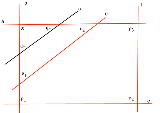
Figure 1: This shows a setup of intersecting branes in type IIA that can yield $D$-term inflation. We have a total of 6 branes. Brane $c$ is our inflationary brane. Branes $a$ and $b$ give rises to the necessary Yukawa coupling between the inflaton and the waterfall field. Branes $e$ and $f$ are there to ensure that the $D$-term potential has a flat direction. This flat direction is broken by the $F$-term potential but this is planckian suppressed. Finally, brane $d$ is necessary for the anomalies to cancel, it plays no other role during the inflationary era. $S$, $\phi_{\pm}$, $\delta_{1,2}$ and $\rho_{1,2,3}$ are the various bifundamental fields at each intersections. Also note that this picture is a two dimensional depiction of a configuration that actually lives in six curved dimensions.

The $U(1)$ gauge group living on each brane stack will contribute a $D$-term to the Lagrangian. We thus obtain the $D$-term potential

$$V_{D} = g_{c}^{2}(|\phi_{+}|^{2}-|\phi_{-}|^{2}-\xi_{c})^{2}+g_{a}^{2}(|\phi_{-}|^{2}-|\delta_{2}|^{2}-|S|^{2}+|\rho_{3}|^{2}-\xi_{a})^{2}$$ (6)

$$+g_{b}^{2}(|S|^{2}+|\delta_{1}|^{2}-|\phi_{+}|^{2}-|\rho_{1}|^{2}-\xi_{b})^{2}+g_{d}^{2}(|\delta_{2}|^{2}-|\delta_{1}|^{2}-\xi_{d})^{2}$$

$$+g_{e}^{2}(|\rho_{1}|^{2}-|\rho_{2}|^{2}-\xi_{e})^{2}+g_{f}^{2}(|\rho_{2}|^{2}-|\rho_{3}|^{2}-\xi_{f})^{2}\;,$$

where $g_{a,b,c,d,e,f}$ are the gauge couplings of the gauge theories on the three branes, and $\xi_{a,b,c,d,e,f}$ are the Fayet-Iliopoulos terms. These FI-terms are set by the angles between the various branes, and thus are functions of the topological wrapping numbers of the branes and of the complex structure moduli (in Type IIA; Kähler moduli in Type IIB) (see e.g. [23] for a recent discussion). Since we have not dealt with the details of how the moduli are fixed, we cannot solve for these moduli. But there are known mechanisms which are believed to provide a very large number of vacua, each of which has different values for the vevs of the moduli. Relying on this type of statistics, we will treat the FI-terms as tunable parameters (the tuning would occur by selecting a particular metastable vacuum to expand around).

For simplicity we set $\xi_{d}=\delta_{1}=\delta_{2}=0$. We choose the $c$ brane stack as our inflationary potential, and we have

$$V_{\rm{inf}}^{D} = g_{c}^{2}(|\phi_{+}|^{2}-|\phi_{-}|^{2}-\xi_{c})^{2}\;,$$

$$V_{\rm{rest}}^{D} = g_{a}^{2}(|\phi_{-}|^{2}-|S|^{2}+|\rho_{3}|^{2}-\xi_{a})^{2}+g_{b}^{2}(|S|^{2}-|\phi_{+}|^{2}-|\rho_{1}|^{2}-\xi_{b})^{2}$$ (7)

$$+g_{e}^{2}(|\rho_{1}|^{2}-|\rho_{2}|^{2}-\xi_{e})^{2}+g_{f}^{2}(|\rho_{2}|^{2}-|\rho_{3}|^{2}-\xi_{f})^{2}\,.$$

The flat direction is the path in field space along which the variation $\delta(|S|^{2})=\delta(|\rho_{1,2,3}|^{2})=r^{2}$ and $V_{\rm{rest}}^{D}$ is constant . This flat direction constitutes our inflaton.

A Yukawa coupling will arise from a worldsheet instanton stretching over the triangle generated by the three intersecting branes $a$, $b$ and $c$ or $d$:

$$W_{\rm{yuk}}=\lambda_{\phi}S\phi_{+}\phi_{-}+\lambda_{\delta}S\delta_{1}\delta_{2}\;.$$ (8)

Due to gauge invariance, these are the only two renormalizable terms in the superpotential containing these fields. The only Yukawa coupling relevant to the flatness of our inflaton direction is

$$W_{2}={\lambda_{2}\over M_{pl}}S\rho_{1}\rho_{2}\rho_{3}\;.$$ (9)

Note that this coupling is Planck-suppressed because it arises from a “square” in the quiver diagram, rather than a triangle. Higher suppressions are easily allowed by simply choosing more hidden sectors branes such that the flat direction is described by a polygon with more sides. Since the uplifting of the flat directions can be suppressed sufficiently, we will simply drop this term for the moment. And since we are still on a flat-direction of $V_{\rm{rest}}^{D}$, we will set this term to zero as well. We will take canonical Kähler potential for these open string fields Neglecting planckian corrections and setting $\delta_{1,2}=0$, the F-term potential in this model is:

$$V_{F}=\left(\lambda_{\phi}^{2}(|\phi_{+}|^{2}|\phi_{-}|^{2}+|S|^{2}(|\phi_{+}|^{2}+|\phi_{-}|^{2}))+V_{F,\rm{other}}\right)$$ (10)

where $V_{F,\rm{other}}$ is the constant potential from all other F-term SUSY-breaking sectors. In order to have $D$-term inflation we need $F\ll D$. Although this is a working assumption throughout this paper, it could be relaxed and one could have an $F$ and $D$ term of the same order (however, crucial details of the inflaton potential would change in this case). So we will assume the $F$-term potential is subdominant and we will drop it for the rest of this discussion (note that one cannot have a strictly vanishing $F$-term when the $D$-term is non-vanishing in supergravity).

We will work in the regime where the inflaton vev is always smaller than the string/Planck-scale, as well as below the masses of the moduli. As such, we are justified in ignoring gravitational corrections to the Kähler potential, and in using an effective field theory approach with excited strings and moduli integrated out. It is possible that these constraints can be relaxed consistently with inflation, but we will assume them in order to obtain a simple and standard framework. Our scenario for inflation is thus very “field theoretic,” and in fact can be implemented in effective field theory without necessarily relying on its string origin and motivation. Note that it is possible to have some moduli unstable during inflation as long as their effects on the inflationary predictions are under control and that the moduli stabilize at a phenomenologically viable value at the end of inflation.

Note that, a priori, nothing picked out $S$ as the inflaton. It is the initial conditions and the existence of the appropriate flat directions which picks out the appropriate field to act as the inflaton. Also we should emphasize that this model differs from the originally proposed $D$-term inflation model [10] since the inflaton field is in a non-vectorlike representation. The tree-level potential is

$$V_{\rm{tree}}=g^{2}(|\phi_{+}|^{2}-|\phi_{-}|^{2}-\xi)^{2}+\lambda_{\phi}^{2}(|\phi_{+}|^{2}|\phi_{-}|^{2}+|\phi_{+}|^{2}|S|^{2}+|S|^{2}|\phi_{-}|^{2})\;.$$ (11)

The global supersymmetric minimum for this potential occurs at $|\phi_{+}|^{2}=\xi$, $\phi_{-}=S=0$. However, for $|S|>S_{C}={g\sqrt{2\xi}\over\lambda}$, the non-vanishing minimum of the potential is at $\phi_{+}=\phi_{-}=0$. This potential is thus of the hybrid form, with $S$ the inflaton field and $\phi_{+}$ the waterfall field. But one should remember that the actual inflationary path involves more than just the field $S$. In some sense we may thus regard this as a multi-inflaton model, where $S$ is the inflaton which dictates when the waterfall field starts rolling.

For $|S|>S_{C}$, we can thus set $\phi_{\pm}=0$ and write an effective potential for $S$. This potential will have a one-loop correction of Coleman-Weinberg form, yielding

$$V_{eff}(S) =g_{c}^{2}\xi^{2}\left[1+{g_{c}^{2}\over 8\pi^{2}}\log\left({\lambda_{\phi}^{2}|S|^{2}\over\Lambda^{2}}\right)+{g_{d}^{2}\over 8\pi^{2}}\log\left({\lambda_{\delta}^{2}|S|^{2}\over\Lambda^{2}}\right)\right]\;,$$

$$\approx g^{2}\xi^{2}\left[1+{g^{2}\over 4\pi^{2}}\log\left({\lambda^{2}|S|^{2}\over\Lambda^{2}}\right)\right]\;,$$ (12)

where we have taken $g_{c}\sim g_{d}\equiv g$ and $\lambda_{\phi}\sim\lambda_{\delta}\equiv\lambda$ in the second line. Note that the one-loop contribution is dominated by the $S$ dependence. This is the case because the Coleman-Weinberg contribution comes from the splitting of boson and fermion masses. But if we are on a flat direction of $V_{\rm{rest}}^{D}$, then the boson masses are not split by these $D$-terms (the FI contribution is cancelled by the contribution from the vevs of the fields). The only contribution to boson/fermion mass splitting comes from $V_{\rm{inf}}^{D}$, and only $S$ couples to these fields via the Yukawa coupling to generate the fermion mass. So for practical purposes now, $S$ is acting as our inflaton. Note also that any pair of fields that couples to $S$ through a Yukawa coupling will contribute to the Coleman-Weinberg potential . In our case we have two pairs $\phi_{\pm}$ and $\delta_{1,2}$.

Although this standard form of the potential has been widely discussed in cosmology literature [25], it is not trivial to obtain this form in string theory. For example, one typically avoids a large tree-level mass for the inflaton by imposing a discrete symmetry which protects it; it is more difficult to find such a symmetry in string construction. In this intersecting brane model construction, the inflaton appears as an open string field in a non-vectorlike representation and hidden sector gauge invariance protects it from a tree-level mass.

When $|S|=S_{c}$, the waterfall field $\phi_{+}$ becomes tachyonic and begins to condense. As usual in hybrid inflation, this condensation brings a rapid end to inflation. In this case, the condensation of $\phi_{+}$ field causes brane recombination, in which the brane stacks $b$ and $c$ deform and bind to each other in order to minimize their energy. In general one has to worry about whether or not the effective field theory approximation is valid for large values of the Fayet-Iliopoulos term. But we are assuming the limit $\xi\ll m_{S}$, in which case the field theory limit should be valid.

Finally, note that this model predicts the formation of stable cosmic strings at the end of inflation from the spontaneous symmetry breaking of the $U(1)$. As we will see, the experimental bound on the cosmic string is the biggest phenomenological constraint on $D$-term inflation although a simple and natural extension of the model can easily solve the problem.

3.2 Phenomenological Status of D-term Inflation

$D$-term inflation is a fairly robust model that has been extensively studied in the literature (see [26, 27] and references therein for some detailed analysis). In this section, we remind the reader of the simplest story. The $D$-term inflationary potential is

$$V=V_{0}\left(1+\alpha\ln\frac{\lambda s^{2}}{\Lambda^{2}}\right)\;,$$ (13)

where the height of the potential is set by the FI term $V_{0}=g^{2}\xi^{2}$, $\alpha=g^{2}/4\pi^{2}$ is the loop factor and we have defined $s\equiv|S|$. In the slow-roll regime, we can solve for the inflaton field in terms of number of efolds $N$. Using $-Hdt=dN$, one has

$$3H\dot{s}=-\frac{\partial V}{\partial s}\;,$$

$$3H^{2}\frac{\partial s}{\partial N}=\frac{2V_{0}\alpha}{s}\;,$$ (14)

with can be solved approximately for constant $H\approx\sqrt{\frac{V_{0}}{3M_{p}^{2}}}\sim\frac{g\xi}{\sqrt{3}M_{p}}$

$$\frac{s^{2}-s_{0}^{2}}{2}=\frac{2V_{0}\alpha}{3H^{2}}N\;.$$ (15)

The term on the right side is just proportional to $g^{2}M_{p}^{2}$. Given a $g^{2}$ that is not too small, this term will in general dominate over the $s_{0}^{2}$ and this is the limit that we are going to work in [28]. Note that in the opposite limit where $s^{2}\approx s^{2}_{0}\sim|S_{c}|^{2}$, we can still match the data although the observables will now depend on $\lambda$. We require that the initial value of $s$ (which minimally corresponds to 60 efolds) satisfy the following hierarchy of scales for the effective field theory approach to be valid

$$s^{2} \ll m_{\Phi}^{2}\lower 3.01385pt\hbox{$\;\stackrel{{\scriptstyle\textstyle<}}{{\sim}}\;$}m_{\rm{str}}^{2}\ll M_{p}^{2}\;,$$ (16)

where $m_{\Phi}$ is the mass scale of the string moduli and $m_{\rm{str}}$ is the string scale. We note here that we expect a spread in the masses of the moduli (see for e.g [29] where they study the spectrum of moduli masses via random matrix techniques). In order for inflation to go through unmodified, we probably need the value of the inflaton to be lower than most masses of the moduli which might be a stronger requirement than taking it to be smaller than string scale. Supposing that we have no more than 60 efolds, we get that the initial vev of $s$ is of order $s^{2}\sim 6g^{2}M_{P}^{2}$. One could potentially satisfy the needed hierarchy of scale with $g^{2}\sim 10^{-2}$ or $10^{-3}$.

With subplanckian vev for $s$, we will have negligible tensor/scalar ratio $r$. Since this is slow-roll, we expect negligible non-gaussianities and a negligible running of the spectral index. Hence the main three observables are the power spectrum, the spectral index and the cosmic string tension:

$$P_{\mathcal{R}} = \left.\frac{1}{24\pi^{2}M_{p}^{4}}\frac{V}{\epsilon}\right|_{k=aH}=\frac{N}{3}\frac{\xi^{2}}{M_{p}^{4}}\;,$$ (17)

$$n \approx 1+2\eta=1-\frac{1}{N}\;,$$ (18)

$$G\mu \sim \frac{\xi}{M_{p}^{2}}\;.$$ (19)

The first two are evaluated 55 efolds before the end of inflation and the cosmic string tension comes from the end of inflation when the waterfall field condenses. First, we find that the spectral index is $0.98$ which is within $\sim 2\sigma$ range of WMAP3 year data [30]. The power spectrum is measured to be $P_{\mathcal{R}}\sim 10^{-9}$ from which we get that the scale of inflation is of order of the GUT scale

$$\xi\sim 10^{-5}M_{p}^{2}\sim(10^{15}\,{\rm GeV})^{2}\;,$$ (20)

which gives a cosmic string tension of $G\mu\sim 10^{-5}$ which is well in excess of the current experimental bounds $G\mu\lower 3.01385pt\hbox{$\;\stackrel{{\scriptstyle\textstyle<}}{{\sim}}\;$}2\times 10^{-7}$ [31].

In this intersecting brane model setup, one can naturally avoid the production of long-lived cosmic strings entirely by taking one of the gauge groups to be non-abelian. Alternatively, one can also avoid the production of stable cosmic strings by having multiple waterfall fields $\phi_{+}^{i}$ in the bifundamental (this will occur in our toy model if $I_{bc}>1$). In either situation, the vacuum manifold will have trivial $\Pi_{1}$ and the produced cosmic strings will be either of the electroweak type for a local non-abelian symmetry or semilocal for a global non-abelian symmetry [32]. Both type of strings are generically unstable thus permitting them to decay and avoid any conflict with observation [33]. Unfortunately, this resolution of the cosmic string problem will also remove any possible observable signatures of cosmic strings. It is argued that there is a region of the parameter space for which a complete fit of the model including the contribution of the cosmic strings to the power spectrum is possible [34]. In this case it would then be possible to retain an observable cosmic string signature which is consistent with current experiments.

It is interesting to note that, because generically these hidden sector branes will have non-trivial topological intersection with the visible sector branes, the Standard Model can be heated directly by open string degrees of freedom. In contrast, the current models of string inflation (for example, brane inflation) heat the visible sector through gravitation degrees of freedom. We will see that this different feature has implications for baryogenesis.

Finally, we can quantify how much fine-tuning is needed in order not to spoil the slow-roll conditions. Although we have enough scalar fields to make the $D$-term flat, we will still generate $F$-term contribution to the potential from the quartic Yukawa superpotential. Since the log grows very slowly for large $s$, these contributions might ruin the slow-roll condition. During inflation we have $\rho_{i}^{2}+\xi_{j}\sim S^{2}$. From the superpotential (9), we will generate a term $\sim\frac{\lambda_{2}^{2}}{M_{p}^{2}}S^{6}$ as well as lower dimensional terms. Note that lower dimensional term are suppressed by factor of $\xi/M_{p}$ which we have assume are all small ($\xi_{c}$ is the biggest one of the FI terms and it is itself much smaller than $M_{p}$) and therefore the most dangerous term is $S^{6}$.

Now in general a term like $\frac{\lambda_{n}^{2}S^{2n+2}}{M_{p}^{2n-2}}$ will contribute to the $\eta$ parameter (see [35] for a discussion of the importance of these type of terms in $D$-term inflation):

$$\eta\sim\lambda_{n}^{2}(2n+2)(2n+1)\frac{S^{2n}}{V_{0}M_{p}^{2n-4}}\;,$$ (21)

taking $S^{2}\propto 6g^{2}M_{p}^{2}$ at 55 efolds before the end of inflation and the definition of the power spectrum (17). We find that requiring $\eta<10^{-2}$ put the following constraints on $g^{2}$ and $\lambda_{n}^{2}$.

$$\lambda_{n}^{2}(g^{2})^{n-1}<\frac{P_{\mathcal{R}}10^{-2}}{6^{n}(2n+1)(2n+2)}\;.$$ (22)

In our simplest model ($n=2$), we get an $S^{6}$ term which requires a fine-tuning

$$\lambda_{2}^{2}g^{2}<10^{-13}\;.$$ (23)

This could be satisfied if we had $\lambda_{2}\sim g\sim 10^{-3}$. Note that the flat direction can easily arise from a polygon with more sides in our intersecting brane setup. In this case, the $F$-term will come with additional $M_{pl}^{2}$ suppression which reduces this fine-tuning. In any case, we expect gravitational corrections to the Kähler potential to yield potential terms of the form $\Delta V\sim({|S|^{2}\over M_{pl}^{2}})^{n}\langle V_{F,\rm{other}}\rangle$. For low-scale supersymmetry breaking we expect $\langle V_{F,\rm{other}}\rangle\ll V_{0}$ and these corrections will be small. For higher-scale $F$-term supersymmetry breaking, one would have to cancel these corrections against the Yukawa terms. This would be an $\eta$ problem, but if the $F$-term is large than this model can no longer be considered a purely $D$-term inflationary model.

We see from (22) that by using a polygon with enough sides ($n$= 5 should do) one can effectively eliminate the needed fine-tuning. Hence it is possible to brane engineer a flat direction. It is also worth noting that the $\lambda_{2}$ Yukawa coupling is generated by worldsheet instantons, which generally are exponentially suppressed by $\exp(-A/l_{s}^{2})$, where $A$ is the area of the string worldsheet stretching between the brane stacks forming the polygon. In the large volume limit (where known moduli-stabilization schemes are under control), one would expect $A>1$ in string units, implying that the coefficient $\lambda_{2}$ should be relatively small.

On the down side, $g^{2}$ should really be replaced by $\sum g^{2}$ in the case where there are multiple Yukawa couplings between $S$ and other fields. Hence the fine-tuning in equation (22) should be done on every one of the gauge coupling constant that appears in the Coleman-Weinberg potential. Remember that equation (22) was obtained assuming $g_{c}\sim g_{d}$ and so we need to fine-tune both coupling constants.

Finally, since this model is really a multiple fields inflationary scenario, one might expect that isocurvature perturbations will be generated by the fluctuations of the $\rho_{i}$ and these perturbations might modify our fit to the data. These would come from coupling between the $\rho_{i}$ and $S$ in the $F$-term and since we are arguing that these should be small, we expect the isocurvature perturbations to be small as well.

3.3 More complicated/generic setups

This setup is perhaps the simplest version of our scenario which would arise in intersecting brane models, but it is not necessarily the most generic. One might expect, for example, that the various stacks could contain multiple parallel branes (non-Abelian gauge groups) and that the various stacks could have $|I_{xy}|>1$ (more than one multiplet in the various bifundamentals). We will see that these more generic setups provide new constraints, but also new phenomenological features.

The first serious worry is the possibility of multiple waterfall fields for the inflaton potential (the $D$-term potential associated with the $c$ brane stack in our previous example). One source of new waterfall fields would be additional branes stacks with topological intersection with the brane stack $c$. Another source would be multiple topological intersections (for example, suppose in our previous example that we had $I_{bc}>1$). If there exists a new brane stack $g$ with non-trivial topological intersection with $c$, then the new $D$-term potential will be of the form

$$V_{D}=g^{2}(|\phi^{i}_{+}|^{2}-|\phi^{j}_{-}|^{2}\pm|\rho^{k}|^{2}+...-\xi)^{2}$$ (24)

where $\rho$ is the scalar arising from strings stretching between $g$ and $c$, and the superscripts index our choice of chiral multiplet (if we have multiple chiral multiplets transforming in various bifundamentals). The charge of $\rho$ is determined by the sign of the topological intersection. In this more generic setup, one sees that there can be multiple waterfall fields which could condense, causing $V_{inf}^{D}$ to go to zero. For inflation to occur, it is necessary for every waterfall field to get a mass which stays positive until the inflaton reaches its critical value (and inflation ends). But in general this should not be a problem. Recall that if we have $N$ brane stacks generating $N$ $D$-term equations, we generally have ${\cal O}(N^{2})$ scalars which we can use to find flat directions. Requiring those flat-directions to lift the ${\cal O}(N)$ waterfall fields of $V_{\rm{inf}}^{D}$ should still give us ${\cal O}(N^{2})$ acceptable inflaton directions (modulo the fine-tuning of the signs of intersections numbers to obtain Planck-suppression of Yukawa couplings; for a flat direction given by an $n$-sided polygon, this means a choice of ${\cal O}(n^{2})$ signs).

Another subtlety worth noting arises if one of the gauge groups is non-abelian. In this case there will be non-Abelian $D$-terms of the form

$$V_{r}^{D}=(\sum_{i}\phi_{i}^{\dagger}T_{r}\phi_{i})^{2}$$ (25)

where $T$ is a non-diagonal generator of the gauge group and $\phi_{i}$ is any scalar charged under the non-abelian symmetry (there is no FI-term for these terms). If $G_{c}$ is a non-Abelian group, then one must worry if the presence of the new $D$-term equation will prevent the full $D$-term potential from dropping to zero when $\phi_{+}$ condenses. Indeed, if $\phi_{+}$ is the only waterfall field then $V_{D}^{total}$ will reach an ${\cal O}(1)$ fraction of the original value of $V_{0}$ (due to the non-zero final value of $V_{r}^{D}$). In this case, the waterfall will still end inflation but we would now need to be sure that the cosmological constant at the end of the waterfall is small to match observation. This would require a cancellation between $V_{D}$ (which is an ${\cal O}(1)$ fraction of the inflation scale), and $V_{F}$, which in turn presents an $\eta$-problem which must be resolved by fine-tuning. Since we would have $D$-terms of order $V_{0}$, we would in this case be led to a model of high-scale supersymmetry breaking. But it is important to note that this is only true in the simple example where there is only one waterfall field. If for example, we had $I_{bc}=2$, we would have two waterfall doublet fields $\phi_{+}^{1,2}$. In this case, one can see that by condensing the upper component of the $\phi_{+}^{1}$ and the lower component of $\phi_{-}^{2}$, one can set to zero all of the $D$-terms associated with brane stack $c$ (furthermore, if $I_{ca}=2$, then the inflaton $S$ alone can give mass to all the waterfall fields via generic Yukawa couplings). Another way of phrasing this would be to note that although non-Abelian $D$-terms will give us more constraints than our original ${\cal O}(N)$, higher topological intersection numbers can give us more fields than our original ${\cal O}(N^{2})$, so that we can still find sufficiently many flat directions.

Finally, we briefly discuss a subtlety mentioned in [36]. As they noted, it is potentially difficult to maintain low-energy supersymmetry while simultaneously fixing the FI-terms at a high-scale (i.e., fixing the closed string moduli on which the FI-terms depend at a high scale). If the $U(1)$ associated to the $D$-term is anomalous (with the anomaly fixed by the Green-Schwarz mechanism), then the vector boson becomes massive by eating the axion. However, the axion itself is in the same multiplet as the Kähler moduli, which are assumed fixed at a high scale. If supersymmetry is preserved, then this would imply that the vector multiplet becomes massive at a high-scale, in which case one should not see the $D$-term equation at low energies. One might worry that our scenario would face this difficulty, as the appearance of so many non-vectorlike representations would imply that many $U(1)$’s have some mixed anomalies.

Of course, as noted in [36], this $D$-term picture can be made consistent by some amount of $F$-term supersymmetry breaking, and this amount can be made very small. This picture is completely consistent with our scenario. But one should remember that in our scenario, it is in fact possible to generate many non-anomalous $U(1)$’s. One can see this simply by noting that the number of anomalous $U(1)$’s with anomalies fixed by the Green-Schwarz mechanism is limited by the number of axions present (basically, by the number of size moduli in Type IIB). For every axion, only one $U(1)$ can become massive; if there are more $U(1)$ factors arising from branes than there are axions, the remainder must be non-anomalous. Generally, the non-anomalous $U(1)$’s will not simply be the diagonal subgroup living on a brane stack. Instead, they will arise as a linear combination of various diagonal $U(1)$’s. But nothing in our inflation scenario depended on the fact that each $U(1)$ lived on a brane. We only utilized the fact that for every pair of gauge groups there would generally be matter charged under both groups, and this will be true for linear combinations of these groups as well. So the picture above can go forward as before with each of the $U(1)$’s having no mixed anomalies and arising from a linear combination of the diagonal $U(1)$’s living on the various brane stacks. As long as there exists the appropriate fields with charges to be the inflaton and waterfall (which should arise just as easily for a $U(1)$ which arises from a linear combination), the story goes through as before.

3.4 Preheating and the Gravitino Problem

As was shown in [37, 38], the condensation of the waterfall field which ends hybrid inflation is typically accompanied by tachyonic preheating (as opposed to the usual parametric resonance) in which energy is dumped into the long-wavelength modes of the waterfall field itself. Light scalar fields interacting with the waterfall field will be dragged along into the process of preheating. After a while, we expect these excitations to decay to a bath of fermions and bosons in equilibrium. Since this whole process is happening in a hidden sector, the reheating could be happening in multiple stages and it could take a while (for sufficiently small coupling) to reach the final relativistic bath of Standard Model particles.

This would in turn allow us to lower the temperature of reheating. This is usually needed to avoid the gravitino problem, in which a low mass gravitino is overproduced at the end of inflation and overcloses the universe. This is a serious problem to any theory of inflation with a high scale [39]. It is naturally solved when the reheat temperature is roughly lower than $10^{9}\sim 10^{10}$ GeV for TeV scale supersymmetry breaking. This can be accomplished very simply by having a long multi-stage reheating process where the inflationary energy goes through multiple stages before settling into its final Standard model bath of particles. The details of the reheating process are model dependent as one would need to know exactly how strong are the coupling between the inflaton sector and the Standard Model branes.

Finally, it is possible that density perturbations and/or non-gaussianities can be generated in the preheating era. These were shown to be possible by using second order analysis in [40]. Alternatively, it has been argued that the presence of extra light fields on which the mass of the waterfall field depends can also generate density perturbations at the end of inflation [41]. All of this interesting issues are beyond the scope of the current work and we assume that they change the inflationary prediction only in a subdominant way.

4 Hidden Sector Baryogenesis with Tachyonic Preheating

This scenario for inflation in intersecting brane models can also provide input for baryogenesis. One of the most interesting models of baryogenesis is electroweak baryogenesis [42], in which the mixed anomaly between $U(1)_{B}$ and the weak group $SU(2)_{L}$ creates a non-trivial divergence in the baryon current:

$$\partial_{\mu}J_{B}^{\mu}\propto Tr\,[F_{W}\wedge F_{W}]\;.$$ (26)

Electroweak sphaleron processes can thus lead to microscopic baryon generation. If the electroweak phase transition is first order, then this transition provides the departure from thermal equilibrium necessary for the generation of a net baryon asymmetry.

One of the reasons for the great interest in this mechanism is that it is determined by physics at accessible (or soon to be accessible) energy scales and thus can make definite predictions which can be tested. In this regard it is almost too successful; EWBG in the Standard Model is already ruled out by LEP data, and in the MSSM it is tightly constrained into a very narrow window. These constraints largely arise from the necessity for the EWPT to be first order: in the Standard Model one needs $m_{higgs}<70$ GeV, and in the MSSM one needs $m_{higgs}<120$ GeV (the bounds from LEP establish $m_{higgs}>114$ GeV). In addition, the requirement that sufficient CP violation be provided by the Higgs sector provides further constraints (for an overview of all of these constraints, see [43] and references therein).

Thus, an interesting offshoot proposal of EWBG has been electroweak tachyonic preheating [44]. In this model, the electroweak phase transition is a cold transition which occurs at the end of hybrid inflation. The waterfall field which ends inflation is the Higgs field, which simultaneously breaks the electroweak symmetry. Such a fast cold transition will necessarily occur outside thermal equilibrium. Furthermore, tachyonic preheating [37, 38, 44] will robustly dump energy into the long-wavelength modes of the fields coupled to the waterfall field as it condenses. These modes can thus excite the electroweak sphalerons necessary for the generation of a baryon asymmetry. This proposal is a novel alternative which offers a chance to realize EWBG despite the constraints on the EWPT. However, it necessarily requires low-scale inflation (in fact, electroweak scale), which is accompanied by its own set of constraints in order to generate the correct scale of density perturbations.

On a parallel track, a recently proposed model of hidden sector baryogenesis [45] realizes a mechanism reminiscent of EWBG in a context very natural to intersecting brane models. In HSB, mixed anomalies between a hidden sector gauge group $G$ and $U(1)_{B}$ result in a non-trivial divergence for the baryon current

$$\partial_{\mu}J_{B}^{\mu}\propto Tr\,[F_{G}\wedge F_{G}]\;.$$ (27)

As a result, sphaleron/instanton processes in the hidden $G$ sector can generate a baryon asymmetry in much the same way that electroweak sphalerons generate it in EWBG. These hidden sectors are numerous and appear generically in intersecting brane models, and they generically have mixed anomalies with both $U(1)_{B}$ and $U(1)_{B-L}$. Since any one of these groups can generate a baryon asymmetry if it has a strongly first order phase transition, and it only takes one for the mechanism to work, HSB provides a robust mechanism for generating a baryon asymmetry in IBMs. The generic appearance of $[U(1)_{B-L}G^{2}]$ mixed anomalies implies that HSB generates a $B-L$ asymmetry as well, which cannot be washed out by electroweak sphalerons.

We now see that HSB fits naturally into our $D$-term IBM inflation story through tachyonic preheating. The waterfall field $\phi_{+}$ is charged under $G_{b}$ and $G_{c}$, the gauge groups living on brane stacks $b$ and $c$. As it condenses, the group $G_{b}\times G_{c}$ will break to a subgroup $G$. Via tachyonic preheating, energy will be dumped into the long-wavelength modes of fields coupled to $\phi_{+}$, and in particular into the gauge fields of $G_{b}\times G_{c}$, which are simultaneously becoming massive. As mentioned earlier, brane stacks $b$ and $c$ will generically intersect with the visible sector brane stack carrying $U(3)_{qcd}$. The diagonal $U(1)$ subgroup of this will be $U(1)_{B}$, and thus we will generically have a non-zero mixed anomaly of the form $[U(1)_{B}G_{b,c}^{2}]$ (in fact, there will generically be a $[U(1)_{B-L}G_{b,c}^{2}]$ mixed anomaly as well). We may write this as

$$\partial_{\mu}J_{B}^{\mu}\propto C_{b}Tr[F_{G_{b}}\wedge F_{G_{b}}]+C_{c}Tr[F_{G_{c}}\wedge F_{G_{c}}]\;.$$ (28)

Long wavelength modes of the $G_{b}\times G_{c}$ gauge fields will excite sphalerons of the hidden sector, which will in turn generate a baryon asymmetry via the anomaly, as in HSB (and analogous to electroweak tachyonic preheating baryogenesis). Moreover, this transition will occur at the symmetry breaking scale of the $G_{b}\times G_{c}$ sector, which can be relatively high. So in this scenario, inflation does not need to be at a very low scale, avoiding one of the constraints of electroweak tachyonic preheating.

A prototype for this might be an example where $G_{b}=U(1)$ and $G_{c}=U(2)$ or $Sp(1)$, which would be very similar to electroweak breaking. In the original works on electroweak tachyonic preheating, numerical simulations demonstrated that when the electroweak gauge theory is broken by condensation of the waterfall field, tachyonic preheating would indeed dump energy into the gauge field, which in turn would excite sphalerons and (accompanied by C and CP violation) generate a baryon asymmetry. Such a mechanism can certainly work in the HSB context for the gauge theories arising in intersecting brane models as well, provided that C and CP violation are present (they should appear generically in the hidden sector gauge theory; whether or not they are of the correct magnitude is a detailed model dependent question which one must answer hidden sector by hidden sector). But one still must ensure that after tachyonic preheating, when the radiation has thermalized, the sphalerons are shut off. Otherwise, the sphalerons could wash out the generated baryon asymmetry. An estimate for the condition for this washout to be suppressed is

$${T_{RH}\over\langle\phi_{+}\rangle}<1$$ (29)

where $T_{RH}\sim({30V_{0}\over\pi^{2}g_{*}})^{1\over 4}$ is the (maximum) reheat temperature and $g_{*}$ is the number of relativistic degrees of freedom into which energy can be dumped. For our case, we have $V_{0}=g^{2}\xi^{2}$. Since we also have $|\phi_{+}|^{2}=\xi$ after condensation, we get

$${T_{RH}\over\langle\phi_{+}\rangle}\sim{1.3\over g_{*}^{1\over 4}}g^{1\over 2}$$ (30)

For $g_{*}\sim 10$ and $g\leq 0.9$, sphalerons will certainly be suppressed after tachyonic preheating, and the generated asymmetry will not be washed out.

One might instead consider the case where $G_{b,c}$ are both abelian groups. In this case the hidden sector will no longer have the complicated vacuum structure which allowed the sphaleron processes, which in turn generated the baryon asymmetry via the anomaly. An intriguing alternative would be the non-equilibrium generation of charged particle/anti-particle pairs and currents in the hidden sector. For a $U(1)$ hidden sector gauge group, we have

$$\partial_{\mu}J_{B}^{\mu}\propto\int F_{G}\wedge F_{G}=\int E_{G}\cdot B_{G}$$ (31)

As energy from the waterfall field is dumped into the hidden sector, one expects the generation of charged particle/anti-particle pairs which would in turn lead to non-trivial hidden sector electric and magnetic fields. The lack of thermal equilibrium, and violation of B, C and CP imply that all Sakharov conditions are satisfied, and thus that one can generate a baryon asymmetry through the anomaly. But it is a non-trivial task to understand the precise mechanism by which departure from equilibrium, combined with C and CP violation, can generate the required non-zero $\int E\cdot B$. Furthermore, it would be a technical exercise to verify that, as the gauge field becomes massive during the waterfall stage, the electric and magnetic fields are suppressed sufficiently quickly to shut-down the baryon-violating processes before thermalization, in order to avoid washout of the asymmetry. These interesting questions are beyond the scope of this work, though we hope to revisit them.

5 The Generation of Neutrino Masses

The condensation of the waterfall field breaks a gauge symmetry and the scale of this symmetry breaking can be around $10^{14}-10^{16}$GeV. This gauge symmetry can thus be used to protect the Majorana mass of right handed neutrino and this mass scale can be used to generate light neutrino masses via the seesaw mechanism [46]. The light neutrino mass can be written as $m^{\rm light}_{\nu}=-M^{D}_{\nu}{1\over M_{Maj}}{M^{D}_{\nu}}^{T}$, where $M^{D}_{\nu}$ is the Dirac neutrino mass which arises from the $\lambda_{\nu}L\nu^{c}H$ coupling and the magnitude of this mass is typically of the order of the weak scale. The Majorana mass arises from the $f\nu^{c}\nu^{c}\phi$ interaction and the magnitude of this mass is of the order of the symmtery breaking scale where the MSSM is generated. After including the magnitudes of these mass scales in the seesaw formula, one can find that the heaviest light neutrino mass can be 0.1 eV or less. The precise values and the flavor structures of the Dirac and Majorana couplings will generate the neutrino mixing angles and masses to satisfy the experimental results. Here, we are interested to see how the light neutrino masses are connected to our inflation mechanism.

We can consider this scenario in an effective field theory approach. Here, the field $\phi$ which appears in the Majorana interaction is the waterfall field. The full gauge symmetry is protected until the waterfall field condenses and this symmetry can be, e.g., $SU(3)_{c}\times SU(2)_{L}\times U(1)_{T_{3R}}\times U(1)_{B-L}$, with both $\phi$ and $\nu^{c}$ are charged under $T_{3R}$ and ${B-L}$. $U(1)_{T_{3R}}\times U(1)_{B-L}$ is then broken down to $U(1)_{Y}$ due to the condensation of $\phi$. $T_{3R}$ charges are assigned to the fields in such a way so that fields have the correct hypercharge. The Majorana mass term develops once the waterfall field develops a VEV. In this process both $B-L$ and $T_{3R}$ symmetries are spontaneously broken and the baryon asymmetry that is produced due to the $[U(1)_{B-L}G^{2}]$ anomaly is not washed out due to electroweak sphaleron process.

We can also consider this scenario in an IBM implementation of $D$-term inflation which we have discussed here. For example, we consider the case where the $c$ brane stack which we discussed earlier is in fact the leptonic stack, on which $U(1)_{L}$ lives. Generically we expect the $T_{3R}$ stack to have non-vanishing topological intersection with the the hidden sector stack $b$ (on which $\phi=\phi_{+}$ also ends, see Fig. 2).

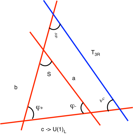
Figure 2: One can simply generate the neutrino masses at the end of inflation by making stack $c$ the leptonic brane with gauge symmetry $U(1)_{L}$. We then need both stacks $b$ and $c$ to intersect the $T_{3R}$ brane in order to generate the correct Yukawa coupling. Here in addition to the previous inflaton sector fields, we have the right-handed neutrino $\nu^{c}$ and an exotic $\xi$.

Assuming that the right-handed neutrinos arise from multiplets living on the intersection of the leptonic and $T_{3R}$ brane stacks, we now find that allowed renormalizable Yukawa couplings are

$$W_{yuk.}=\lambda S\phi\phi_{-}+f\phi\xi\nu^{c}$$ (32)

If we denote by $U(1)_{b}$ the diagonal subgroup of $G_{b}$, then we can define the hypercharge group $U(1)_{Y}=U(1)_{B-L}+U(1)_{T_{3R}}+U(1)_{b}+...$, under which SM particles have correct hypercharge and $\phi$ and $\xi$ have vanishing hypercharge. The extra Yukawa coupling will not affect the inflation potential significantly, as the scalars in the $\xi$ and $\nu^{c}$ multiplets have vanishing expectation value during inflation. $\xi$ is a Majorana field whose mass is protected by the $T_{3R}$ symmetry which can also break around the scale where $B-L$ breaks down. The Majorana mass of $\nu^{c}$ arises from a tree-level interaction with the fermionic component of $\xi$ appearing as the intermediate line. We thus find $m_{\nu^{c}}\sim f^{2}\langle\phi\rangle^{2}/M_{\xi}$, where $M_{\xi}$ is $\sim$ GUT scale and is, therefore, of the right magnitude to generate the light neutrino mass.

It is interesting to note that lepton asymmetry in this model can be generated by CP-violating out-of-equilibrium decays of right handed neutrinos [47]. This asymmetry is obtained via the tree and loop contributions in the decay of the lightest right-handed Majorana neutrino into leptons and scalar Higgs. The electroweak sphaleron process then converts the lepton asymmetry to a baryon asymmetry.

Although hidden sector baryogenesis and the generation of mass for the neutrinos can both fit nicely and simultaneously into this picture of $D$-term inflation in IBMs, it is not necessary for both mechanisms to appear simultaneously. For example, we can consider IBMs where the baryon asymmetry is generated at the end of inflation by HSB associated with tachyonic preheating, while the neutrino masses are generated by unconnected dynamics. Similarly, we can consider models where the condensation of the waterfall field generates the neutrino masses, but baryogenesis is dominated by contributions other than HSB (including perhaps leptogenesis of the form discussed above).

6 Conclusion

We have developed a scenario of $D$-term inflation which appears to arise quite straightforwardly in the context of intersecting brane models. In this case, the inflaton $S$ lives in a chiral multiplet arising from strings stretching between two hidden sector branes at their point of intersection. The waterfall field has a similar origin. A noteworthy feature of this type of inflation is that it can quite naturally generate a baryon asymmetry in the visible sector at the end of inflation via the recently proposed hidden sector baryogenesis mechanism [45]. One can also easily generalize this model to additionally generate Majorana masses for neutrinos. One of the puzzles of cosmological evolution has been the origin of the various required scales. One would need to understand where the scale of the Majorana masses arises from, and depending on the mechanism of baryogenesis, also the origin of the scale at which one departs from equilibrium. The scenario we discuss here ties both of these scales directly to the scale of inflation; to our knowledge, it is the only scenario to achieve this. Further, both high and low scale supersymmetry breakings are compatible with baryogenesis which can happen in the hidden sector or via leptogenesis.

Although a key motivation for this scenario comes from the general features of intersecting brane models, this scenario can be thought of purely in terms of effective field theory. As such, it may have wider application. Of course, we think of this as a scenario instead of a true “model” since we have not illustrated with a specific construction. Thus far, it has proven relatively difficult to generate specific examples of intersecting brane models in compactifications in which all closed string moduli are fixed, although some work on this subject has been done [2]. There are many difficulties in combining an intersecting brane model with the features necessary for fixing moduli, such as fluxes and non-perturbative corrections, but it seems to us that these problems are technical in nature; there is no clear reason why shouldn’t be able to stabilize moduli in some compactification with an IBM.

More specifically, there are two main working assumptions in this paper that remain to be worked out in detail in order to achieve a consistent string theory embedding of this scenario. One assumption is that there exists a consistent moduli stabilization scheme where the $D$-term energy dominates over the $F$-term. Secondly, we have not included any quantum corrections to the FI term which may depend on the inflaton field. One might expect that the quantum corrections are suppressed since the inflaton field is a bifundamental living at an intersection separated from the brane that generates the dominant FI term during inflation. We leave an investigation of these issues for future work [48].

To the extent that one thinks of this as inflation in an intersecting brane model (as opposed to a more generic effective field theoretic setting), it obviously relies on the existence of many such moduli-stabilized IBMs. It would of course be very interesting to understand specific examples of such moduli-stabilized IBMs, and to see if this type of inflation scenario can be realized. Along these lines, another very interesting problem is to better understand which branes and features are generic in the class of moduli-stabilized intersecting brane models, beyond the more well-understood set of toroidal orientifold constructions.

References

- [1] R. Blumenhagen, L. Goerlich, B. Kors and D. Lust, JHEP 0010, 006 (2000) [arXiv:hep-th/0007024]; C. Angelantonj, I. Antoniadis, E. Dudas and A. Sagnotti, Phys. Lett. B 489, 223 (2000) [arXiv:hep-th/0007090]; R. Blumenhagen, L. Goerlich, B. Kors and D. Lust, Fortsch. Phys. 49, 591 (2001) [arXiv:hep-th/0010198]; G. Aldazabal, S. Franco, L. E. Ibanez, R. Rabadan and A. M. Uranga, J. Math. Phys. 42, 3103 (2001) [arXiv:hep-th/0011073]; G. Aldazabal, S. Franco, L. E. Ibanez, R. Rabadan and A. M. Uranga, JHEP 0102, 047 (2001) [arXiv:hep-ph/0011132]; M. Cvetic, G. Shiu and A. M. Uranga, Nucl. Phys. B 615, 3 (2001) [hep-th/0107166]; M. Cvetic, P. Langacker and G. Shiu, Nucl. Phys. B 642, 139 (2002) [hep-th/0206115]; R. Blumenhagen, V. Braun, B. Kors and D. Lust, arXiv:hep-th/0210083; A. M. Uranga, Class. Quant. Grav. 20, S373 (2003) [arXiv:hep-th/0301032]; M. Cvetic, P. Langacker, T. j. Li and T. Liu, Nucl. Phys. B 709, 241 (2005) [arXiv:hep-th/0407178]; M. Cvetic and T. Liu, Phys. Lett. B 610, 122 (2005) [arXiv:hep-th/0409032]; C. Kokorelis, arXiv:hep-th/0410134; C. M. Chen, T. Li and D. V. Nanopoulos, Nucl. Phys. B 732, 224 (2006) [hep-th/0509059]; B. Dutta and Y. Mimura, Phys. Lett. B 633, 761 (2006) [arXiv:hep-ph/0512171]; M. R. Douglas and W. Taylor, JHEP 0701, 031 (2007) [arXiv:hep-th/0606109].
- [2] F. Marchesano and G. Shiu, Phys. Rev. D 71, 011701 (2005) [arXiv:hep-th/0408059]; F. Marchesano and G. Shiu, JHEP 0411, 041 (2004) [arXiv:hep-th/0409132]; M. Cvetic, T. Li and T. Liu, Phys. Rev. D 71, 106008 (2005) [arXiv:hep-th/0501041]; R. Blumenhagen, M. Cvetic, P. Langacker and G. Shiu, Ann. Rev. Nucl. Part. Sci. 55, 71 (2005) [arXiv:hep-th/0502005]; J. Kumar and J. D. Wells, JHEP 0509, 067 (2005) [arXiv:hep-th/0506252]; C. M. Chen, V. E. Mayes and D. V. Nanopoulos, Phys. Lett. B 633, 618 (2006) [arXiv:hep-th/0511135]; C. M. Chen, T. Li and D. V. Nanopoulos, Nucl. Phys. B 740, 79 (2006) [arXiv:hep-th/0601064]; J. Kumar and J. D. Wells, arXiv:hep-th/0604203.
- [3] F. Quevedo, Class. Quant. Grav. 19, 5721 (2002) [arXiv:hep-th/0210292]; C. P. Burgess, arXiv:hep-th/0606020; S. H. Henry Tye, arXiv:hep-th/0610221; J. M. Cline, arXiv:hep-th/0612129; R. Kallosh, arXiv:hep-th/0702059;
- [4] G. R. Dvali and S. H. H. Tye, Phys. Lett. B 450 (1999) 72 [arXiv:hep-ph/9812483].
- [5] S. H. S. Alexander, Phys. Rev. D 65, 023507 (2002) [arXiv:hep-th/0105032]; G. R. Dvali, Q. Shafi and S. Solganik, arXiv:hep-th/0105203; C. P. Burgess, M. Majumdar, D. Nolte, F. Quevedo, G. Rajesh and R. J. Zhang, JHEP 0107 (2001) 047 [arXiv:hep-th/0105204]; J. Garcia-Bellido, R. Rabadan and F. Zamora, JHEP 0201, 036 (2002) [arXiv:hep-th/0112147].
- [6] E. Silverstein and D. Tong, Phys. Rev. D 70 (2004) 103505 [arXiv:hep-th/0310221]; M. Alishahiha, E. Silverstein and D. Tong, Phys. Rev. D 70 (2004) 123505 [arXiv:hep-th/0404084].
- [7] S. Kachru, R. Kallosh, A. Linde, J. M. Maldacena, L. McAllister and S. P. Trivedi, JCAP 0310, 013 (2003) [arXiv:hep-th/0308055].
- [8] R. Bean, S. E. Shandera, S. H. Henry Tye and J. Xu, arXiv:hep-th/0702107.
- [9] C. P. Burgess, J. M. Cline, H. Stoica, and F. Quevedo, JHEP, 09:033, 2004. arXiv:hep-th/0403119.
- [10] P. Binetruy and G. R. Dvali, Phys. Lett. B 388, 241 (1996) [arXiv:hep-ph/9606342]; E. Halyo, Phys. Lett. B 387, 43 (1996) [arXiv:hep-ph/9606423].
- [11] F. G. Marchesano Buznego, arXiv:hep-th/0307252.
- [12] S. B. Giddings, S. Kachru and J. Polchinski, Phys. Rev. D 66, 106006 (2002) [arXiv:hep-th/0105097]; S. Kachru, R. Kallosh, A. Linde and S. P. Trivedi, Phys. Rev. D 68, 046005 (2003) [arXiv:hep-th/0301240]; O. DeWolfe, A. Giryavets, S. Kachru and W. Taylor, JHEP 0507, 066 (2005) [arXiv:hep-th/0505160].
- [13] E. Silverstein, arXiv:hep-th/0106209; A. Maloney, E. Silverstein and A. Strominger, arXiv:hep-th/0205316; E. Silverstein, arXiv:hep-th/0407202.
- [14] N. Arkani-Hamed, A. G. Cohen and H. Georgi, Phys. Lett. B 513, 232 (2001) [arXiv:hep-ph/0105239]; Z. Chacko, H. S. Goh and R. Harnik, Phys. Rev. Lett. 96, 231802 (2006) [arXiv:hep-ph/0506256].
- [15] J. P. Hsu, R. Kallosh and S. Prokushkin, JCAP 0312 (2003) 009 [arXiv:hep-th/0311077]; F. Koyama, Y. Tachikawa and T. Watari, [arXiv:hep-th/0311191]; H. Firouzjahi and S. H. H. Tye, Phys. Lett. B 584 (2004) 147 [arXiv:hep-th/0312020]; J. P. Hsu and R. Kallosh, JHEP 0404 (2004) 042 [arXiv:hep-th/0402047].
- [16] R. Kallosh and M. Soroush, arXiv:hep-th/0612057.
- [17] C. P. Burgess, R. Kallosh and F. Quevedo, JHEP 0310, 056 (2003) [arXiv:hep-th/0309187].
- [18] K. Choi, A. Falkowski, H. P. Nilles and M. Olechowski, Nucl. Phys. B 718, 113 (2005) [arXiv:hep-th/0503216]; S. P. de Alwis, Phys. Lett. B 626, 223 (2005) [arXiv:hep-th/0506266].
- [19] G. Villadoro and F. Zwirner, Phys. Rev. Lett. 95, 231602 (2005) [arXiv:hep-th/0508167].
- [20] Ph. Brax, C. van de Bruck, A. C. Davis, S. C. Davis, R. Jeannerot and M. Postma, JCAP 0701, 026 (2007) [arXiv:hep-th/0610195].
- [21] A. Achucarro, B. de Carlos, J. A. Casas and L. Doplicher, JHEP 0606, 014 (2006) [arXiv:hep-th/0601190].
- [22] B. de Carlos, J. A. Casas, A. Guarino, J. M. Moreno and O. Seto, arXiv:hep-th/0702103.
- [23] G. Villadoro and F. Zwirner, JHEP 0603, 087 (2006) [arXiv:hep-th/0602120].
- [24] D. Lust, P. Mayr, R. Richter and S. Stieberger, Nucl. Phys. B 696, 205 (2004) [arXiv:hep-th/0404134]; M. Bertolini, M. Billo, A. Lerda, J. F. Morales and R. Russo, Nucl. Phys. B 743, 1 (2006) [arXiv:hep-th/0512067].
- [25] D. H. Lyth and A. Riotto, Phys. Rept. 314, 1 (1999) [arXiv:hep-ph/9807278].
- [26] M. ur Rehman, V. N. Senoguz and Q. Shafi, arXiv:hep-ph/0612023.
- [27] D. H. Lyth, arXiv:hep-th/0702128.
- [28] D. H. Lyth and A. Riotto, Phys. Lett. B 412, 28 (1997) [arXiv:hep-ph/9707273]; J. R. Espinosa, A. Riotto and G. G. Ross, Nucl. Phys. B 531, 461 (1998) [arXiv:hep-ph/9804214].
- [29] R. Easther and L. McAllister, JCAP 0605, 018 (2006) [arXiv:hep-th/0512102].
- [30] D. N. Spergel et al. [WMAP Collaboration], arXiv:astro-ph/0603449.
- [31] M. Wyman, L. Pogosian and I. Wasserman, Phys. Rev. D 72, 023513 (2005) [Erratum-ibid. D 73, 089905 (2006)] [arXiv:astro-ph/0503364].
- [32] T. Vachaspati and A. Achucarro, Phys. Rev. D 44, 3067 (1991); A. Achucarro and T. Vachaspati, Phys. Rept. 327, 347 (2000) [Phys. Rept. 327, 427 (2000)] [arXiv:hep-ph/9904229].
- [33] J. Urrestilla, A. Achucarro and A. C. Davis, Phys. Rev. Lett. 92, 251302 (2004) [arXiv:hep-th/0402032]; O. Seto and J. Yokoyama, Phys. Rev. D 73, 023508 (2006) [arXiv:hep-ph/0508172]; C. M. Lin and J. McDonald, Phys. Rev. D 74, 063510 (2006) [arXiv:hep-ph/0604245]; Ph. Brax, C. van de Bruck, A. C. Davis and S. C. Davis, Phys. Lett. B 640, 7 (2006) [arXiv:hep-th/0606036]; J. Rocher and M. Sakellariadou, JCAP 0611, 001 (2006) [arXiv:hep-th/0607226]; R. Jeannerot and M. Postma, JCAP 0607, 012 (2006) [arXiv:hep-th/0604216].
- [34] J. Rocher and M. Sakellariadou, Phys. Rev. Lett. 94, 011303 (2005) [arXiv:hep-ph/0412143].
- [35] C. F. Kolda and J. March-Russell, Phys. Rev. D 60, 023504 (1999) [arXiv:hep-ph/9802358].
- [36] P. Binetruy, G. Dvali, R. Kallosh and A. Van Proeyen, Class. Quant. Grav. 21, 3137 (2004) [arXiv:hep-th/0402046].
- [37] G. N. Felder, J. Garcia-Bellido, P. B. Greene, L. Kofman, A. D. Linde and I. Tkachev, Phys. Rev. Lett. 87, 011601 (2001) [arXiv:hep-ph/0012142].
- [38] G. N. Felder, L. Kofman and A. D. Linde, Phys. Rev. D 64, 123517 (2001) [arXiv:hep-th/0106179].
- [39] M. Kawasaki, F. Takahashi and T. T. Yanagida, Phys. Rev. D 74, 043519 (2006) [arXiv:hep-ph/0605297]; M. Endo, M. Kawasaki, F. Takahashi and T. T. Yanagida, Phys. Lett. B 642, 518 (2006) [arXiv:hep-ph/0607170].
- [40] N. Barnaby and J. M. Cline, Phys. Rev. D 73, 106012 (2006) [arXiv:astro-ph/0601481]; N. Barnaby and J. M. Cline, arXiv:astro-ph/0611750.
- [41] D. H. Lyth and A. Riotto, Phys. Rev. Lett. 97, 121301 (2006) [arXiv:astro-ph/0607326]; L. Leblond and S. Shandera, JCAP 0701, 009 (2007) [arXiv:hep-th/0610321].
- [42] V. A. Kuzmin, V. A. Rubakov and M. E. Shaposhnikov, Phys. Lett. B 155, 36 (1985).
- [43] C. Balazs, M. Carena, A. Menon, D. E. Morrissey and C. E. M. Wagner,
- [44] J. Garcia-Bellido, M. Garcia Perez and A. Gonzalez-Arroyo, Phys. Rev. D 67, 103501 (2003) [arXiv:hep-ph/0208228]; J. Smit and A. Tranberg, JHEP 0212, 020 (2002) [arXiv:hep-ph/0211243]; J. Garcia-Bellido, M. Garcia-Perez and A. Gonzalez-Arroyo, Phys. Rev. D 69, 023504 (2004) [arXiv:hep-ph/0304285]; A. Tranberg and J. Smit, JHEP 0311, 016 (2003) [arXiv:hep-ph/0310342]; A. Tranberg and J. Smit, JHEP 0608, 012 (2006) [arXiv:hep-ph/0604263]; A. Tranberg, J. Smit and M. Hindmarsh, JHEP 0701, 034 (2007) [arXiv:hep-ph/0610096].
- [45] B. Dutta and J. Kumar, Phys. Lett. B 643, 284 (2006) [arXiv:hep-th/0608188].
- [46] P. Minkowski, Phys. Lett. B 67, 421 (1977); T. Yanagida, in proc. of KEK workshop, eds. O. Sawada and S. Sugamoto (Tsukuba, 1979); M. Gell-Mann, P. Ramond and R. Slansky, in Supergravity, eds. P. van Nieuwenhuizen and D. Z. Freedman (North-Holland, Amsterdam, 1979); R. N. Mohapatra and G. Senjanović, Phys. Rev. Lett. 44, 912 (1980).
- [47] M. Fukugita and T. Yanagida, Phys. Lett. B 174, 45 (1986).
- [48] Work in progress.