Instability of de Sitter brane and horizon entropy in a 6D braneworld

Abstract

We investigate thermodynamic and dynamical stability of a family of six-dimensional braneworld solutions with de Sitter branes. First, we investigate thermodynamic stability in terms of de Sitter entropy. We see that the family of solutions is divided into two distinct branches: the high-entropy branch and the low-entropy branch. By analogy with ordinary thermodynamics, the high-entropy branch is expected to be stable and the low-entropy branch to be unstable. Next, we investigate dynamical stability by analysing linear perturbations around the solutions. Perturbations are decomposed into scalar, vector and tensor sectors according to the representation of the 4D de Sitter symmetry, and each sector is analysed separately. It is found that when the Hubble expansion rates on the branes are too large, there appears a tachyonic mode in the scalar sector and the background solution becomes dynamically unstable. We show analytically that the onset of the thermodynamic instability and that of the dynamical instability exactly coincide. Therefore, the braneworld model provides a new example illustrating close relations between thermodynamic and dynamical instability.

I Introduction

The braneworld scenario, in which matter fields are confined on a brane in higher dimensional spacetime, has been one of the most exciting subjects in the research into the early universe. As the early universe is supposed to have experienced a rather high-energy epoch, studies of the dynamics of the early universe might reveal as yet undiscovered imprints of extra dimensions to us.

In our previous studies Mukohyama:2005yw ; Yoshiguchi:2005nn ; Sendouda:2006bn we considered a $6$-dimensional braneworld model with one or two $3$-branes. The shape and the size of the extra dimensions are stabilized by magnetic flux of a $U(1)$ gauge field and the geometry on each brane is either Minkowski or de Sitter. Since all moduli are stabilized, it is expected that the $4$-dimensional Einstein gravity should be recovered on each brane. In Ref. Mukohyama:2005yw we analyzed how the Hubble expansion rate on each brane changes when the brane tension changes. The resulting relation between the Hubble expansion rate and the brane tension can be considered as an effective Friedmann equation, which in turn defines an effective Newton’s constant. It was shown that at sufficiently low Hubble expansion rates, the effective Newton’s constant resulting from this analysis agrees with that inferred by simply integrating extra dimensions out. The stability of this model was investigated in Ref. Yoshiguchi:2005nn ; Sendouda:2006bn , where it was shown that the background with Minkowski branes is always stable against linear perturbations with axisymmetry in the extra dimensions.

The purpose of this paper is to study stability of backgrounds with de Sitter branes. This is not just a trivial extension of the previous analysis but actually results in a qualitatively different picture. Indeed, the background becomes unstable when the Hubble expansion rate becomes too large. (For other models, see for example Frolov:2003yi ; Contaldi:2004hr ; Bousso:2002fi ; Martin:2004wp ; Krishnan:2005su .) We shall obtain the critical expansion rate at which the background becomes unstable and interpret this behavior in terms of de Sitter thermodynamics.

Spacetimes with horizons appear mysterious in many respects. An observer does not have causal contact with any events beyond a horizon and, in this sense, the horizon separates the region behind it from the observer’s side. Thus, from the observer’s viewpoint, information beyond the horizon is completely irrelevant (as far as classical evolution in the observable region is concerned). This, nothing but a restatement of the definition of horizons, suggests a coarse-grained description of a physical system in or of a spacetime with horizons. It is therefore not totally surprising that a spacetime with horizons exhibits properties analogous to those of thermodynamics. Indeed, in the case of black holes such properties are known as black hole thermodynamics .

Black hole entropy, defined as one quarter of horizon area in Planck units, is central to black hole thermodynamics. The second law of black hole thermodynamics states that black hole entropy never decreases classically. Its semi-classical extension, known as the generalized second law, states that the sum of black hole entropy and matter entropy does not decrease. These second laws are direct analogues of the second law of ordinary thermodynamics and restrict directions in which a physical system involving black holes can evolve. In ordinary thermodynamics it is due to the second law that entropy can be used to analyze stability of a thermodynamic system. Therefore, the validity of the second law of black hole thermodynamics suggests potential use of black hole entropy to guess stability of a system including black holes or objects (branes, strings, rings, and so on) Braden:1990hw ; Maeda:1993ap ; Prestidge:1999uq ; Gubser:2000mm ; Gubser:2000ec ; Reall:2001ag ; Arcioni:2004ww . (Also, for a review see e.g. Harmark:2007md and references therein.)

The close connection between black hole event horizons and thermodynamics can be extended to event horizons in cosmological models with a positive cosmological constant Gibbons:1977mu . The de Sitter thermodynamics includes concepts of de Sitter temperature and de Sitter entropy.

In this paper we shall extend the de Sitter entropy to our braneworld set-up with two extra dimensions and use it to “predict” the stability condition for the backgrounds with de Sitter branes. Intriguingly, the simple “prediction” by de Sitter entropy completely agrees with the result of rather involved analysis of linear perturbations. This is really non-trivial and may be considered as an evidence showing the usefulness of de Sitter entropy and, more generally, holographic principle Strominger:2001pn ; Bousso:2002ju .

The rest of this paper is organized as follows. In Sec. II we briefly review our $6$-dimensional braneworld model with de Sitter branes. In Sec. III we study thermodynamic stability of the spacetime by using entropy. In Sec. IV, in order to investigate dynamical stability we consider linear perturbation around the background solution. In Sec. V we summarize the results and discuss them.

II 6D brane model with warped flux compactification

We consider a 6D Einstein–Maxwell system described by the action

$$I=\frac{1}{16\pi G_{6}}\int\mathrm{d}^{6}x\sqrt{-g}\left(R-2\Lambda_{6}-\frac{1}{2}F_{MN}F^{MN}\right),$$ (1)

where $\Lambda_{6}$ is the 6D bulk cosmological constant $(\Lambda_{6}>0)$ and $F_{MN}=\partial_{M}A_{N}-\partial_{N}A_{M}$ is the field strength of the $U(1)$ gauge field $A_{M}$ introduced to stabilize the extra dimensions. (We use units with $G_{6}=1$ where $G_{6}$ is the 6D Newton’s constant unless otherwise noted.) The braneworld solution is

$$\mathrm{d}s^{2}_{6}=\tilde{r}^{2}\mathrm{d}s^{2}_{4}+\frac{\mathrm{d}\tilde{r}^{2}}{\tilde{f}(\tilde{r})}+\tilde{f}(\tilde{r})\mathrm{d}\tilde{\phi}^{2},\quad A_{M}\mathrm{d}x^{M}=\tilde{A}(\tilde{r})\mathrm{d}\tilde{\phi},$$ (2)

where

$$\tilde{f}(\tilde{r})=k-\frac{\Lambda_{6}}{10}\tilde{r}^{2}-\frac{\tilde{\mathcal{M}}}{\tilde{r}^{3}}-\frac{\tilde{b}^{2}}{12\tilde{r}^{6}},\quad\tilde{A}(\tilde{r})=\frac{\tilde{b}}{3\tilde{r}^{3}},$$ (3)

and $\mathrm{d}s^{2}_{4}$ is the metric of the 4-dimensional spacetime with a constant curvature $k$, i.e. de Sitter ($k>0$), Minkowski ($k=0$), or anti-de Sitter (AdS) ($k<0$) spacetime. Without loss of generality, we can normalize $k$ to $\pm 1$ except for the Minkowski ($k=0$) case. We consider the range of parameters in which $\tilde{f}(\tilde{r})$ has two positive roots, and locate two 3-branes at the positions of the two roots $\tilde{r}=r_{\pm}$ $(0<r_{-}<r_{+})$. We call the branes at $\tilde{r}=r_{\pm}$ the $\tilde{r}_{\pm}$-branes, respectively. The tension of each brane determines a conical deficit in the extra dimensions. To be precise, the period of the angular coordinate ($\tilde{\phi}\sim\tilde{\phi}+\Delta\phi$) is given by

$$\Delta\phi=\frac{2\pi-8\pi\sigma_{+}}{|\tilde{f}^{\prime}(r_{+})/2|}=\frac{2\pi-8\pi\sigma_{-}}{|\tilde{f}^{\prime}(r_{-})/2|},$$ (4)

where $\sigma_{\pm}$ are tensions of the branes at $\tilde{r}=r_{\pm}$.

This braneworld model includes two compact extra dimensions and two 3-branes at $\tilde{r}=r_{\pm}$ with the tensions $\sigma_{\pm}$. For $k=+1$, the geometries on the brane at $\tilde{r}=r_{\pm}$ are the 4D de Sitter spacetimes with the Hubble expansion rates $h_{\pm}=1/r_{\pm}$, respectively. For $k=0$, the brane geometry is the Minkowski spacetime. In each case the energy scale on each brane is scaled by the warp factor $\tilde{r}^{2}$ depending on the position of the brane. The role of the $U(1)$ field is to stabilize extra dimensions with magnetic flux.

Now, for later convenience we re-scale coordinates and parameters of the geometry with the 4D Hubble parameter $h_{+}$ on the $r_{+}$-brane in the following manner:

$$\tilde{r}\to\frac{r}{h},\quad\tilde{\phi}\to h\phi,\quad\tilde{\mathcal{M}}\to\frac{\mathcal{M}}{h^{5}},\quad\tilde{b}\to\frac{b}{h^{4}},\quad\tilde{x}^{\mu}\to hx^{\mu},$$ (5)

where we have omitted the subscript “$+$” of $h_{+}$ and the tilde denotes re-scaled quantities. After this re-scaling, we obtain

$$\mathrm{d}s^{2}_{6}=r^{2}g_{\mu\nu}\mathrm{d}x^{\mu}\mathrm{d}x^{\nu}+\frac{\mathrm{d}r^{2}}{f(r)}+f(r)\mathrm{d}\phi^{2},\quad A_{M}\mathrm{d}x^{M}=A(r)\mathrm{d}\phi,$$ (6)

where

$$f(r)=h^{2}-\frac{\Lambda_{6}}{10}r^{2}-\frac{\mathcal{M}}{r^{3}}-\frac{b^{2}}{12r^{6}},\quad A(r)=\frac{b}{3r^{3}}.$$ (7)

Here $g_{\mu\nu}$ is the metric of the 4D de Sitter spacetime with the Hubble parameter $h$. The metric function now satisfies $f(\alpha)=f(1)=0$, where $\alpha\equiv r_{-}/r_{+}$ is the ratio of the warp factors at the branes and, at the same time, describes how the geometry of the 2D extra dimensions is warped. Note that in the special case $\alpha=1$ the geometry is not warped but locally a round sphere.

Advantages of this re-scaled parameterization are as follows. First, the new parameters and coordinates remain finite and regular in the limit where the geometries on the branes become Minkowski. Second, since the warp factor evaluated at the $r_{+}$-brane is unity ($r=1$), many quantities rooted in these coordinates have physical meaning as observables measured by observers on the $r_{+}$-brane. As we will see later, a Kaluza–Klein (KK) mass measured on the $r_{+}$-brane remains finite in the $\alpha\to 0$ limit, while that on the $r_{-}$-brane diverges. Hence, it is useful (in particular for the purpose of numerical calculations) to use quantities measured on the $r_{+}$-brane. Of course, if we know the value of a quantity measured on the $r_{+}$ brane then we can easily obtain the corresponding value measured on the $r_{-}$-brane by multiplying the warp factor $\alpha$, e.g., $h_{-}=h_{+}/\alpha$, $m^{2}_{-}=m^{2}_{+}/\alpha^{2}$, and so on, where $m_{\pm}$ is the KK mass observed on the $r_{\pm}$-brane.

We introduce another convenient parameter $\beta$. From $f(\alpha)=f(1)=0$ we obtain the relation

$$h^{2}+\frac{b^{2}}{12\alpha^{3}}=\frac{\Lambda_{6}(\alpha^{4}+\alpha^{3}+\alpha^{2}+\alpha+1)}{10(\alpha^{2}+\alpha+1)}.$$ (8)

Since $b^{2}\geq 0$, the Hubble parameter $h$ has a maximum value $h_{\mathrm{max}}(\alpha)$ for a given $\alpha$. Hence we define $\beta$ by

$$\beta\equiv\frac{h^{2}}{h_{\mathrm{max}}(\alpha)^{2}}=\frac{10(1+\alpha+\alpha^{2})}{\Lambda_{6}(1+\alpha+\alpha^{2}+\alpha^{3}+\alpha^{4})}h^{2},$$ (9)

which is the squared Hubble parameter $h^{2}$ on the $r_{+}$-brane normalized by $h_{\mathrm{max}}(\alpha)$. Alternatively, $\beta$ could be defined as $h_{-}^{2}$ normalized by its maximum value, but the two definitions are actually equivalent. Thus, $\beta$ describes how much the $4$D part of the metric is curved. When $\beta=0$, the 4D spacetime becomes flat . In contrast, in the maximal case ($\beta=1$), the flux disappears: $b=0$.

For a fixed bulk cosmological constant $\Lambda_{6}$ and a fixed discrete parameter $k$ ($=0,1$), the solution is locally parameterized by the two parameters $b$ and $\mathcal{M}$. However it is more convenient to use the pair of dimension-less parameters $(\alpha,\beta)$, both of which run over the finite interval $[0,1]$. This parameterization includes both $k=1$ ($0<\beta\leq 1$) and $k=0$ ($\beta=0$) cases, and treats the de Sitter and the Minkowski branes in the common way.

In the following sections we use the parameters ($\alpha$, $\beta$) and the coordinates ($r$, $\phi$, $x^{\mu}$) to describe the background geometry.

III thermodynamic stability

As stated in the introduction, one of the main subjects in this paper is the close connection between thermodynamic and dynamical properties of spacetimes. In particular, we shall see exact agreement between thermodynamic and dynamical stabilities for the $6$-dimensional brane world solutions described in the previous section. In this section we discuss thermodynamic stability by using the de Sitter entropy. We also point out the close relation between the specific heat and the effective Friedmann equation.

III.1 Entropy argument

In the $4$-dimensional Einstein gravity, a de Sitter space has entropy given by one quarter of the area of the horizon Gibbons:1977mu . This is an analogue of the well-known black hole entropy and has been the basis of holographic arguments for de Sitter spaces Strominger:2001pn ; Bousso:2002ju .

In the 6D braneworld background solution, each point in the 2D extra dimensions corresponds to a 4D de Sitter space. Therefore, we shall define the de Sitter entropy in our context by one quarter of the area of the cosmological horizon integrated over the extra dimensions, i.e., one quarter of the volume of the 4-dimensional surface foliated by de Sitter horizons:

$$S\equiv\frac{\mathcal{A}_{4}}{4G_{6}},$$ (10)

where $\mathcal{A}_{4}$ is the 4-dimensional volume given by

$$\mathcal{A}_{4}=\frac{4\pi}{h^{2}}\int_{\alpha}^{1}\!\!r^{2}\mathrm{d}r\int^{\Delta\phi}_{0}\!\!\mathrm{d}\phi=\frac{4\pi}{3h^{2}}(1-\alpha^{3})\Delta\phi,$$ (11)

and $G_{6}$ is the 6D Newton’s constant. Note that, for the convenience of the discussion, we have temporarily restored $G_{6}$ in this paragraph. Actually, it is easy to show that this definition agrees with the definition of the 4D de Sitter entropy that observers on each brane would adopt. The area of the de Sitter horizon and the Newton’s constant on the $r_{\pm}$-brane are, respectively, given by

$$\mathcal{A}_{+}=\alpha^{-2}\mathcal{A}_{-}=\frac{4\pi}{h^{2}}$$ (12)

and

$$\frac{1}{G_{\mathrm{N}+}}=\frac{\alpha^{2}}{G_{\mathrm{N}-}}=\frac{1}{G_{6}}\int_{\alpha}^{1}\!\!r^{2}\mathrm{d}r\int^{\Delta\phi}_{0}\!\!\mathrm{d}\phi.$$ (13)

Thus, the 4D de Sitter entropies on the $r_{\pm}$-branes are

$$S_{\pm}\equiv\frac{\mathcal{A}_{\pm}}{4G_{\mathrm{N}\pm}},$$ (14)

respectively. These do indeed agree with the above definition based on the horizon area integrated over the extra dimensions:

$$S_{+}=S_{-}=S.$$ (15)

In the 4D picture, the integration over extra dimensions is taken care of by the above formula of the 4D Newton’s constant (13). Since the three different definitions agree, we have a unique definition of de Sitter entropy in our braneworld set-up.

To investigate the thermodynamic stability of the system, it is useful to consider the de Sitter entropy as a function of conserved quantities. The family of solutions described in the previous section has three conserved quantities: the total magnetic flux and the tensions of two branes. The total magnetic flux $\Phi$ is given by

$$\Phi=\int_{\alpha}^{1}F_{r\phi}\mathrm{d}r\int_{0}^{\Delta\phi}\mathrm{d}\phi=\frac{b}{3\alpha^{3}}(\alpha^{3}-1)\Delta\phi.$$ (16)

By Eq. (4), tensions $\sigma_{\pm}$ of the $r_{\pm}$-branes are expressed as

$$\sigma_{\pm}=\frac{2\pi-\kappa_{\pm}}{8\pi},$$ (17)

respectively, where $\kappa_{\pm}$ are defined by

$$\kappa_{+}=-\frac{1}{2}f^{\prime}(1)\Delta\phi,\quad\kappa_{-}=\frac{1}{2}f^{\prime}(\alpha)\Delta\phi.$$ (18)

Since there is one-to-one correspondence between $\sigma_{\pm}$ and $\kappa_{\pm}$, we can consider the de Sitter entropy $S$ as a function of either ($\Phi$, $\sigma_{+}$, $\sigma_{-}$) or ($\Phi$, $\kappa_{+}$, $\kappa_{-}$).

Variables $S$, $\Phi$ and $\kappa_{\pm}$ defined above are proportional to $\Delta\phi$. Because of this trivial dependence, we can eliminate $\Delta\phi$ from all thermodynamic considerations by properly normalizing the variables. In particular, in Appendix A it is shown that the entropy normalized by $\kappa_{-}$, $\widehat{S}\equiv S/\kappa_{-}$, satisfies the differential relation

$$\mathrm{d}\widehat{S}=\left(\frac{\pi}{3h^{4}}\right)\mathrm{d}\eta+\left(\frac{\pi b}{3h^{4}}\right)\mathrm{d}\widehat{\Phi},$$ (19)

where $\eta\equiv\kappa_{+}/\kappa_{-}$, and $\widehat{\Phi}\equiv\Phi/\kappa_{-}$ is the normalized total flux. This means that the normalized entropy $\widehat{S}$ is a function of the two variables $\eta$ and $\widehat{\Phi}$: $\widehat{S}(\eta,\widehat{\Phi})$. Hereafter, $\eta$ and $\widehat{\Phi}$ are to be considered as two independent thermodynamic variables. This accords with the observation made in the previous section: the family of solutions are parameterized by two parameters ($\alpha$, $\beta$) after proper scaling of variables. The angular period $\Delta\phi$ has been eliminated so that $\widehat{S}$, $\eta$ and $\widehat{\Phi}$ do not depend on it.

Note that the normalization factor $1/\kappa_{-}$ is just a fixed constant from the viewpoint of observers on the $r_{+}$-brane since these observers are to see the response of the 4D geometry induced on the $r_{+}$-brane to the change of the tension $\sigma_{+}$ or equivalently, $\kappa_{+}$. In particular, with $\kappa_{-}$ fixed, we have

$$\mathrm{d}\eta=-\frac{8\pi}{\kappa_{-}}\mathrm{d}\sigma_{+}.$$ (20)

Thus, the relation (19) is relevant for observers on the $r_{+}$-brane (but not for those on the $r_{-}$-brane). Alternatively, we could write down a differential relation relevant for observers on the $r_{-}$-brane by normalizing the variables by the factor $1/\kappa_{+}$, which is a constant from the viewpoint of observers on the $r_{-}$-brane. In this sense, we have two conceptually different pictures: one from $r_{+}$-brane perspectives and the other from $r_{-}$-brane perspectives. The result of the thermodynamic stability analysis does not depend on the picture: the result from one picture completely agrees with that from the other picture. In the following, we shall see the thermodynamic stability from the $r_{+}$-brane perspectives. Thus, unless there is a possibility of confusion, we omit the subscripts “$\pm$”.

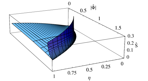
Figure 1: The normalized entropy $\widehat{S}$ as a function of $\eta$ and $\widehat{\Phi}$. Different points on the surface $\widehat{S}=\widehat{S}(\eta,\widehat{\Phi})$ represent different background solutions, and there is no background solution outside the domain of $\widehat{S}(\eta,\widehat{\Phi})$. It is easily seen that $\widehat{S}(\eta,\widehat{\Phi})$ is not single-valued but actually double-valued in some part of its domain. Thus, the family of background solutions has two branches, divided by a critical curve on which some derivatives of $\widehat{S}(\eta,\widehat{\Phi})$ are singular. The high-entropy branch is thermodynamically preferred to the low-entropy branch.

Fig. 1 shows the graph of the normalized de Sitter entropy $\widehat{S}$ as a function of the conserved quantities $\eta$ and $\widehat{\Phi}$. As we can easily see, $\widehat{S}(\eta,\widehat{\Phi})$ is not single-valued but actually double-valued in some part of its domain. It is also easy to see that derivatives of $\widehat{S}(\eta,\widehat{\Phi})$ are singular on a part of the boundary of the domain. We call this part of the boundary of the domain the critical curve. Different points on the surface $\widehat{S}=\widehat{S}(\eta,\widehat{\Phi})$ represent different background solutions, i.e. different spacetimes. (There is no background solution outside the domain of $\widehat{S}(\eta,\widehat{\Phi})$.) Therefore, the critical curve divides the family of solutions into two distinct branches: one with larger $\widehat{S}$ and the other with smaller $\widehat{S}$. We call them the high-entropy branch and the low-entropy branch, respectively. By definition, these two branches merge on the critical curve. Note that in some region of the low-entropy branch, $\widehat{S}(\eta,\widehat{\Phi})$ is single-valued.

If the de Sitter entropy has any physical meaning like entropy in ordinary thermodynamics then the high-entropy branch must be thermodynamically preferred in some sense and must be more stable than the low-entropy branch. The spacetime is marginally stable on the critical curve. These observations are based only on our intuition that the de Sitter entropy should play a role similar to that of entropy in ordinary thermodynamics. Nonetheless, surprisingly, we shall see in the next section that these observations correctly “predict” the result of rather detailed analysis of dynamical stability against linear perturbations.

We now derive an explicit equation describing the critical curve. For this purpose, we consider the coordinate transformation from $(\alpha,\beta)$ defined in the previous section to $(\eta,\widehat{\Phi})$ defined above. As we shall see below, the critical curve is the set of points where this coordinate transformation becomes singular. As noticed in Sec. II, $\alpha$ ($\in(0,1]$)is the ratio of the warp factors of two branes and describes the shape of the two-dimensional extra space. On the other hand $\beta$ ($\in[0,1]$) represents the curvature of 4D de Sitter space normalized by the maximum value $h^{2}_{\mathrm{max}}(\alpha)$ for a given $\alpha$. Since the background solution is uniquely specified by $(\alpha,\beta)$ up to the scaling explained in the previous section, any (properly normalized) quantities can be rewritten as functions of $(\alpha,\beta)$. In particular, we have two single-valued functions $\eta(\alpha,\beta)$ and $\widehat{\Phi}(\alpha,\beta)$ as a map $(\alpha,\beta)\to(\eta,\widehat{\Phi})$. The entropy $\widehat{S}$ is also a single-valued function of $(\alpha,\beta)$ and, thus, the critical curve is determined by vanishing Jacobian determinant of this map:

$$\left|\frac{\partial(\eta,\widehat{\Phi})}{\partial(\alpha,\beta)}\right|=0.$$ (21)

This condition can be solved with respect to $\beta$ to give the following expression for the critical value of $\beta$:

$$\beta_{\mathrm{cri}}(\alpha) =\frac{1}{12(1+\alpha+\alpha^{2})^{2}(1+\alpha+\alpha^{2}+\alpha^{3}+\alpha^{4})}\bigl{[}11+33\alpha+66\alpha^{2}+85\alpha^{3}+90\alpha^{4}+85\alpha^{5}+66\alpha^{6}+33\alpha^{7}+11\alpha^{8}$$ (22)

$$\quad-(1+\alpha)(1+2\alpha+4\alpha^{2}+2\alpha^{3}+\alpha^{4})\sqrt{1+34\alpha^{3}+\alpha^{6}}\bigr{]}.$$

This is the analytic expression for the critical curve. As we see later, $\beta_{\mathrm{cri}}(1)=2/3$ (or, $h^{2}_{\mathrm{cri}}=\Lambda_{6}/9$ and $b^{2}_{\mathrm{cri}}=6h^{2}_{\mathrm{cri}}$) is nothing but the critical value for stabilizing the extra dimensions like in Freund–Rubin compactification Martin:2004wp .

III.2 Effective Newton’s constant

We have seen that the (normalized) de Sitter entropy is not a single-valued function but actually a double-valued function of the conserved quantities $(\eta,\widehat{\Phi})$ in some region of the domain. This observation has led us to a rather natural stability criterion that the high-entropy branch should be stable and that the low-entropy branch should be unstable. This is a global statement: we would not be able to say one of the two branches should be stable or unstable without knowing the existence of the other branch.

In this subsection, we look at the stability from a different viewpoint, considering the effective Friedmann equation investigated in Ref. Mukohyama:2005yw . In particular, we shall see that the thermodynamic stability is equivalent to the positivity of an effective Newton’s constant. Note that, while the thermodynamic stability is a global statement, the positivity of the effective Newton’s constant is a local statement.

In our previous work Mukohyama:2005yw we showed that the 4D Friedmann equation is recovered on the brane at sufficiently low energy as the response of the 4D Hubble expansion rate to the change of the brane tension. To be more precise, for small Hubble expansion rates $h$, $h^{2}$ is expanded as

$$h^{2}=\left.\frac{8\pi G_{\mathrm{N}}}{3}\right|_{\sigma=\sigma_{0}}(\sigma-\sigma_{0})+\mathcal{O}((\sigma-\sigma_{0})^{2}),$$ (23)

where $\sigma$ is the brane tension and the 4D Newton’s constant $G_{\mathrm{N}}$ is obtained by simply integrating extra dimensions out as (13). The constant $\sigma_{0}$ is the value of $\sigma$ for the Minkowski brane ($h=0$) and depends on $\Phi$ and $\sigma_{-}$, which are actually constants from the viewpoint of observers on the $r_{+}$-brane. Note that the 4D Newton’s constant $G_{\mathrm{N}}$ defined as (13) is always positive.

The terms of order $\mathcal{O}((\sigma-\sigma_{0})^{2})$ and higher are small compared with the linear term if the Hubble expansion rate is sufficiently lower than the energy scale set by the bulk cosmological constant. However, for larger $h^{2}$, the higher order corrections become relevant and $h^{2}$ is no longer approximately linear. Moreover, as we can see from Fig. 2, $h^{2}$ is not necessarily an increasing function of the brane tension. Indeed, if $h^{2}$ is larger than a critical value then it is a decreasing function of the brane tension. To make this peculiar behavior more quantitative, let us define the effective Newton’s constant $G_{\mathrm{eff}}$ on the $r_{+}$-brane by

$$G_{\mathrm{eff}}=\frac{3}{8\pi}\left(\frac{\partial h^{2}}{\partial\sigma_{+}}\right)_{\Phi,\sigma_{-}},$$ (24)

and characterize the critical value by $1/G_{\mathrm{eff}}=0$. For $h$ smaller (or larger) than the critical value, $G_{\mathrm{eff}}$ is positive (or negative, respectively).

Note that, since this effective Newton’s constant runs as the Hubble expansion rate $h$ changes, the exact agreement with $G_{\mathrm{N}}$ is met only in the $h^{2}\to+0$ limit. The agreement in this limit itself is a rather non-trivial consequence of the dynamics of bulk spacetime as explicitly shown in Mukohyama:2005yw , but physical interpretation is simple. While $G_{\mathrm{N}}$ was determined via the coefficient of the contribution of the graviton zero mode to the higher dimensional action, $G_{\mathrm{eff}}$ here incorporates contributions of all Kaluza–Klein modes as well as the zero mode. Since Kaluza–Klein contributions are irrelevant at low energies, these two definitions should agree. On the other hand, at high energies the Kaluza–Klein modes become relevant and make $G_{\mathrm{eff}}$ deviate from $G_{\mathrm{N}}$.

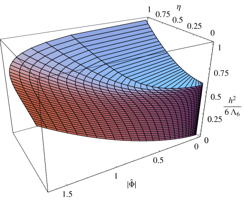
Figure 2: The Hubble expansion rate squared, $h^{2}$, as a function of $\eta$ and $\widehat{\Phi}$. For small $h^{2}$, $(\partial h^{2}/\partial\eta)_{\widehat{\Phi}}$ is negative. However, as $h^{2}$ increases, the slope turns over and $(\partial h^{2}/\partial\eta)_{\widehat{\Phi}}$ becomes positive. (This figure is identical to Fig. 3 of Ref. Mukohyama:2005yw .)

In order to examine the curve $1/G_{\mathrm{eff}}=0$, the following observation is useful:

$$G_{\mathrm{eff}}=-\frac{3}{\kappa_{-}}\left(\frac{\partial h^{2}}{\partial\eta}\right)_{\widehat{\Phi}}=-\frac{6h}{\kappa_{-}}\left|\frac{\partial(h,\widehat{\Phi})}{\partial(\alpha,\beta)}\right|\left/\left|\frac{\partial(\eta,\widehat{\Phi})}{\partial(\alpha,\beta)}\right|\right..$$ (25)

Since $h$ and $\widehat{\Phi}$ are single-valued smooth functions of $(\alpha,\beta)$, the Jacobian $|\partial(h,\widehat{\Phi})/\partial(\alpha,\beta)|$ does not diverge. Hence, $G_{\mathrm{eff}}$ diverges if and only if the denominator $|\partial(\eta,\widehat{\Phi})/\partial(\alpha,\beta)|$ vanishes. This condition is nothing but Eq. (21) characterizing the critical curve, which divides the parameter space of background solutions into the high-entropy branch and the low-entropy branch. Therefore,

Critical curve $$\Leftrightarrow 1/G_{\mathrm{eff}}=0,$$

High-entropy branch $$\Leftrightarrow 1/G_{\mathrm{eff}}>0,$$

Low-entropy branch $$\Leftrightarrow 1/G_{\mathrm{eff}}<0.$$ (26)

Additionally, it is worth mentioning that the effective Newtion’s constant has a connection with thermodynamic quantities on the brane. In the 4D case we can define a temperature of the de Sitter space by the Hubble parameter $H$ as $T=H/2\pi$. Then, in a straightforward manner, the specific heat is given by

$$T\left(\frac{\partial S}{\partial T}\right)=-\frac{2\pi}{G_{\mathrm{N}}H^{2}}.$$ (27)

Now, concerning the 4D de Sitter brane, we consider a specific heat regarding $T=h/2\pi$ as its temperature. From Eq. (19) we obtain

$$T\left(\frac{\partial S}{\partial T}\right)_{\widehat{\Phi},\sigma_{-}}=\kappa_{-}h\left(\frac{\partial\widehat{S}}{\partial h}\right)_{\widehat{\Phi}}=\frac{\pi\kappa_{-}}{3h^{3}}\left(\frac{\partial\eta}{\partial h}\right)_{\widehat{\Phi}}=-\frac{2\pi}{G_{\mathrm{eff}}h^{2}}.$$ (28)

This expression is the same as that of the 4D de Sitter space except for its gravitational “constant.” For the 4D de Sitter brane the sign of the specific heat will change on the critical curve also. Hence, from the viewpoint of the 4D effective theory, we conclude that the effective Newton’s constant on the brane determines thermodynamic properties of the braneworld.

IV Dynamical stability

In the previous section we have discussed the thermodynamic stability of the 6D braneworld model as a property of the background solution. Now let us investigate the dynamical stability of this spacetime. For this purpose, we consider linear perturbations around the background solution. Perturbations are decomposed into scalar-, vector- and tensor-sectors according to the representation of the 4D de Sitter symmetry. If the mass squared of the Kaluza–Klein modes $m^{2}$ is negative, then the corresponding mode is tachyonic and unstable.

Since the background spacetime forms a two-parameter family of solutions, the system of the perturbation equations depends on two parameters ($\alpha$,$\beta$). We investigate the lowest mass squared $m^{2}(\alpha,\beta)$ in each sector as a function of the two parameters in the square domain $0\leq\alpha\leq 1$, $0\leq\beta\leq 1$. Our strategy for attacking the problem is as follows. First, we analytically solve the perturbation equations in the $\alpha=1$ case for arbitrary $\beta\in[0,1]$, and obtain $m^{2}(\alpha=1,\beta)$ on the side $\alpha=1$ of the square domain. Next, by successively applying the relaxation method, we numerically calculate $m^{2}(\alpha,\beta)$ as $\alpha$ changes from $1$ to $0$ for every $\beta$. In each step of the second procedure, the result of the previous step with a slightly larger value of $\alpha$ is used as an initial guess for the relaxation method.

IV.1 Scalar perturbation

As shown in Appendix C, the scalar perturbation with an appropriate gauge choice is given by

$$g_{MN}\mathrm{d}x^{M}\mathrm{d}x^{N} =r^{2}(1+\Phi_{2}Y)g_{\mu\nu}\mathrm{d}x^{\mu}\mathrm{d}x^{\nu}+[1+(\Phi_{1}+\Phi_{2})Y]\frac{\mathrm{d}r^{2}}{f}+[1-(\Phi_{1}+3\Phi_{2})Y]f\mathrm{d}\phi^{2},$$ (29)

$$A_{M}\mathrm{d}x^{M} =(A+a_{\phi}Y)\mathrm{d}\phi,$$

where $Y$ is the scalar harmonics on the 4D de Sitter space satisfying

$$\nabla^{2}Y-m^{2}Y=0.$$ (30)

Here, $\nabla_{\mu}$ is the covariant derivative associated with the 4-dimensional de Sitter spacetime with the Hubble $h$. The Einstein equation and the Maxwell equation are reduced to the following two perturbation equations for $\Phi_{1}$ and $\Phi_{2}$:

$$\Phi^{\prime\prime}_{1}+2\left(\frac{f^{\prime}}{f}+\frac{5}{r}\right)\Phi^{\prime}_{1}-\frac{4\Lambda_{6}}{f}(\Phi_{1}+\Phi_{2})+\frac{m^{2}+18h^{2}}{r^{2}f}\Phi_{1} =0,$$ (31)

$$\Phi^{\prime\prime}_{2}+\frac{4}{r}\Phi^{\prime}_{2}+\frac{m^{2}}{2r^{2}f}(\Phi_{1}+2\Phi_{2}) =0,$$

where the prime denotes the derivative with respect to $r$, and $m^{2}$ is the eigenvalue of the harmonics.

The boundary conditions at $r=\alpha,1$ are obtained by setting the coefficients of $1/f$ in (31) to zero at the brane positions, as in Yoshiguchi:2005nn . Hence we have

$$\left.2f^{\prime}\Phi_{1}^{\prime}-4\Lambda_{6}(\Phi_{1}+\Phi_{2})+\frac{m^{2}+18h^{2}}{r^{2}}\Phi_{1}\right|_{r=\alpha,1}=\left.(\Phi_{1}+2\Phi_{2})\right|_{r=\alpha,1}=0.$$ (32)

An alternative and more rigorous derivation of the boundary conditions is to use the formalism developed in Sendouda:2006bn . The result is

$$\left.f\Phi_{1}\right|_{r=\alpha,1}=\left[2f^{\prime}\Phi_{2}+(f\Phi_{1})^{\prime}\right]_{r=\alpha,1}=0.$$ (33)

These two sets of boundary conditions lead to the same Taylor expansion of $\Phi_{1}$ and $\Phi_{2}$ in the neighborhood of the boundaries and, thus, are equivalent.

In the original coordinate system $(r,\phi)$ the geometry in the $\alpha=1$ limit appears to be singular because two positive roots of $f(r)$ corresponding to the brane positions coincide. Actually, the proper distance between the $r_{\pm}$-branes remains finite and it turns out that the apparent singularity due to coordinate artifacts is removed by appropriate coordinate transformations. Indeed, in the coordinate system ($w$,$\varphi$) defined by

$$w=\frac{2r-(1+\alpha)}{1-\alpha},\quad\varphi=(1-\alpha)\phi,$$ (34)

the geometry is obviously regular in the $\alpha=1$ limit. Note that the coordinate $w$ ranges over the interval $[-1,1]$. Since the branes are always located at $w=\pm 1$ for any $\alpha$ (even for $\alpha=1$), the new coordinate $w$ is more useful for numerical calculation than the original one $r$. Therefore we rewrite the perturbation equation in terms of $w$ as

$$\partial_{w}^{2}\Phi_{1}+2\left\{\frac{\partial_{w}\bar{f}}{\bar{f}}+\frac{5(1-\alpha)}{[(1-\alpha)w+(1+\alpha)]}\right\}\partial_{w}\Phi_{1}-\frac{1}{\bar{f}}(\Phi_{1}+\Phi_{2})+\frac{2\mu^{2}+18h^{2}/\Lambda_{6}}{[(1-\alpha)w+(1+\alpha)]^{2}\bar{f}}\Phi_{1} =0,$$ (35)

$$\partial_{w}^{2}\Phi_{2}+\frac{4(1-\alpha)}{[(1-\alpha)w+(1+\alpha)]}\partial_{w}\Phi_{2}+\frac{\mu^{2}}{[(1-\alpha)w+(1+\alpha)]^{2}\bar{f}}(\Phi_{1}+2\Phi_{2}) =0,$$

where

$$\bar{f}(w)\equiv \frac{f(r)}{\Lambda_{6}(1-\alpha)^{2}}$$ (36)

$$= \frac{1}{40(1-\alpha)^{2}}\left\{-[(1-\alpha)w+(1+\alpha)]^{2}+\frac{4(1+\alpha+\alpha^{2}+\alpha^{3}+\alpha^{4})\beta}{1+\alpha+\alpha^{2}}\right.$$

$$\left.+\frac{32(1+\alpha)[1+\alpha^{2}(1+\alpha^{2}+\alpha^{4})(1-\beta)-(1+\alpha^{3})\beta]}{[(1-\alpha)w+(1+\alpha)]^{3}(1+\alpha+\alpha^{2})}-\frac{256\alpha^{3}(1+\alpha+\alpha^{2}+\alpha^{3}+\alpha^{4})(1-\beta)}{[(1-\alpha)w+(1+\alpha)]^{6}(1+\alpha+\alpha^{2})}\right\}$$

and

$$\mu^{2}=\frac{m^{2}}{2\Lambda_{6}}.$$ (37)

The boundary condition is written as

$$\left.2\partial_{w}\bar{f}\partial_{w}\Phi_{1}-(\Phi_{1}+\Phi_{2})+\frac{2\mu^{2}+18h^{2}/\Lambda_{6}}{[(1-\alpha)w+(1+\alpha)]^{2}}\Phi_{1}\right|_{w=\pm 1} =0,$$ (38)

$$\left.(\Phi_{1}+2\Phi_{2})\right|_{w=\pm 1} =0.$$

IV.1.1 Analytic solution for $\alpha=1$

Now we show the analytic solution for $\alpha=1$. In this case the geometry of the extra dimensions becomes locally a round 2-sphere as in Ref. Freund:1980xh and the warp factor is a constant. Hence, the background spacetime for $\alpha=1$ corresponds to the football-shaped extra dimensions Carroll:2003db ; Garriga:2004tq .

In the $\alpha=1$ limit, the perturbation equations (35) are reduced to

$$(1-w^{2})\partial_{w}^{2}\Phi_{1}-4w\partial_{w}\Phi_{1}-\left(2-\frac{4\mu^{2}}{4-3\beta}\right)\Phi_{1}-\frac{8}{4-3\beta}\Phi_{2} =0,$$ (39)

$$(1-w^{2})\partial_{w}^{2}\Phi_{2}+\frac{2\mu^{2}}{4-3\beta}(\Phi_{1}+2\Phi_{2}) =0.$$

and the boundary conditions are given by

$$\left.-2w(4-3\beta)\Phi^{\prime}_{1}-4\Phi_{2}+(-4+3\beta+2\mu^{2})\Phi_{1}\right|_{w=\pm 1}=0,\quad\left.\Phi_{1}+2\Phi_{2}\right|_{w=\pm 1}=0.$$ (40)

The solution satisfying these boundary conditions is

$$\Phi_{1}^{(\pm)}=-2P_{n}(w)+\frac{4-3\beta}{2\mu^{2}_{(\pm)}}[n(n+1)P_{n}(w)-2wP^{\prime}_{n}(w)],\quad\Phi_{2}^{(\pm)}=P_{n}(w),$$ (41)

up to an overall constant, where $n=0,1,2,\cdots$, and $P_{n}$ is the Legendre function of the first kind. We obtain the mass spectrum of the scalar perturbation as

$$\mu^{2}=\mu_{(\pm)}^{2}\equiv\frac{2-3\beta+n(1+n)(4-3\beta)\pm\sqrt{(2-3\beta)^{2}+12n(1+n)(1-\beta)(4-3\beta)}}{4}.$$ (42)

The mass of the lowest mode is given by

$$\mu^{2}_{(+)}(n=0)=1-\frac{3}{2}\beta.$$ (43)

Thus, for $\beta\geq 2/3$, the lowest $\mu^{2}$ becomes negative and the background spacetime is destabilizedContaldi:2004hr ; Bousso:2002fi ; Martin:2004wp .

IV.1.2 The lowest mass of the KK mode

Now we numerically solve the perturbation equations and obtain the lowest KK mass of the scalar mode for general $\alpha$. Using the analytic solution for $\alpha=1$ as a first initial guess, we solve the problem for a slightly smaller value of $\alpha$ by the relaxation method. Then, as we change $\alpha$ to smaller values towards $0$ step by step, we in turn use the numerical solution of the previous step as an initial guess for the relaxation method and obtain the mass squared for each $\alpha$ and $\beta$.

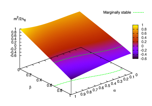
Figure 3: $m^{2}$ for the lowest mode of the scalar perturbation. When $\beta=0$ the 4D spacetime is the Minkowski. As $\beta$ becomes larger (i.e. the 4D Hubble becomes larger), $m^{2}$ decreases and eventually becomes negative beyond some value of $\beta$. The line represents the boundary between the stable and the unstable region, where the massless modes appear.

Fig. 3 shows $m^{2}$ for the lowest mode of the scalar perturbation. For $\beta=0$, which means the 4D spacetime is the Minkowski, we have reproduced the result of our previous study Yoshiguchi:2005nn that there is no unstable (i.e. neither massless nor tachyonic) mode. We find that as $\beta$ becomes larger, namely as the Hubble parameter on the brane becomes larger, $m^{2}$ decreases and eventually becomes negative. Therefore we conclude that when the Hubble on the brane is too large the extra dimensions are destabilized and such configurations are unstable for general $\alpha$. In addition, in the case of vanishing flux ($\beta=1$) the configurations are always unstable.

IV.1.3 The threshold massless mode

Supported by the result shown in Fig. 3, the assumption that $m^{2}$ is a continuous function of $\alpha$ and $\beta$ is made. Hence, it must vanish on the boundary between the stable and unstable regions. In other words, there should appear a massless mode as one moves from the stable/unstable region to the unstable/stable region.

We can actually obtain this threshold massless mode analytically. The general solution of (31) with $m^{2}=0$ is given by

$$\Phi_{1}=\frac{1}{f}\left(\frac{c_{1}}{r^{3}}+\frac{c_{2}}{r^{6}}+c_{3}r^{2}+\frac{c_{4}}{r}\right),\quad\Phi_{2}=\frac{5}{2\Lambda_{6}}\left(4c_{3}+\frac{c_{4}}{r^{3}}\right),$$ (44)

where $c_{i}(i=1,2,3,4)$ are arbitrary constants. By imposing the boundary conditions (33), we will be able to obtain the boundary between the stable and the unstable region on the $(\alpha,\beta)$ plane, where the massless modes appear. The boundary conditions lead to

$$\begin{pmatrix}\alpha^{2}&\alpha^{-1}&\alpha^{7}&\alpha^{4}\\ 1&1&1&1\\ 6\Lambda_{6}\alpha^{6}&12\Lambda_{6}\alpha^{3}&-20b^{2}\alpha^{3}+4\Lambda_{6}\alpha^{11}-120\mathcal{M}\alpha^{6}&-5b^{2}+4\Lambda_{6}\alpha^{8}-30\mathcal{M}\alpha^{3}\\ 6\Lambda_{6}&12\Lambda_{6}&-20b^{2}+4\Lambda_{6}-120\mathcal{M}&-5b^{2}+4\Lambda_{6}-30\mathcal{M}\end{pmatrix}\begin{pmatrix}c_{1}\\ c_{2}\\ c_{3}\\ c_{4}\end{pmatrix}=\begin{pmatrix}0\\ 0\\ 0\\ 0\end{pmatrix},$$ (45)

where $\mathcal{M}$ and $b$ are functions of $(\alpha,\beta)$ determined by $f(\alpha)=f(1)=0$. In order for this equation to allow a non-trivial solution for $(c_{1},c_{2},c_{3},c_{4})$, the determinant of the matrix must vanish. From this condition, we obtain the relation between $(\alpha,\beta)$ as

$$\beta=\beta_{\mathrm{cri}}(\alpha) \equiv\frac{1}{12(1+\alpha+\alpha^{2})^{2}(1+\alpha+\alpha^{2}+\alpha^{3}+\alpha^{4})}\bigl{[}11+33\alpha+66\alpha^{2}+85\alpha^{3}+90\alpha^{4}+85\alpha^{5}+66\alpha^{6}+33\alpha^{7}+11\alpha^{8}$$ (46)

$$\quad-(1+\alpha)(1+2\alpha+4\alpha^{2}+2\alpha^{3}+\alpha^{4})\sqrt{1+34\alpha^{3}+\alpha^{6}}\bigr{]}.$$

This relation is exactly identical with (22), which defines the critical curve on which the high-entropy branch and the low-entropy branch merge. The threshold massless mode divides the whole square $(\alpha,\beta)$-domain into positive and negative $m^{2}$ regions, while the critical curve in Sec. III divides the whole square $(\alpha,\beta)$-domain into high- and low-entropy regions. Therefore, the high-entropy and the low-entropy branches in Fig. 1 exactly agree with the positive and negative $m^{2}$ regions in Fig. 3, respectively. This fact implies that in this spacetime thermodynamically preferred configurations are dynamically stable, while thermodynamically non-preferred ones have tachyonic modes and become dynamically unstable. The onset of dynamical instability coincides with the onset of thermodynamic instability. This is similar to the Gubser–Mitra conjecture for extended black objects Gubser:2000mm ; Gubser:2000ec .

IV.2 Vector perturbation

As shown in Appendix C, the vector perturbation with an appropriate gauge choice is given by

$$g_{MN}\mathrm{d}x^{M}\mathrm{d}x^{N} =r^{2}g_{\mu\nu}\mathrm{d}x^{\mu}\mathrm{d}x^{\nu}+2h_{(\mathrm{T})\phi}V_{(\mathrm{T})\mu}\mathrm{d}x^{\mu}\mathrm{d}\phi+\frac{\mathrm{d}r^{2}}{f}+f\mathrm{d}\phi^{2},$$ (47)

$$A_{M}\mathrm{d}x^{M} =a_{(\mathrm{T})}V_{(\mathrm{T})\mu}\mathrm{d}x^{\mu}+A\mathrm{d}\phi,$$

where $V_{(\mathrm{T})\mu}$ is the vector harmonics on the 4D de Sitter space, which satisfies the transverse condition, $\nabla^{\mu}V_{(\mathrm{T})\mu}=0$. The Einstein equation and the Maxwell equation are reduced to two perturbation equations with respect to $h_{(\mathrm{T})\phi}$ and $a_{(\mathrm{T})}$,

$$\frac{1}{r^{4}}\left[r^{6}\left(\frac{h_{(\mathrm{T})\phi}}{r^{2}}\right)^{\prime}\right]^{\prime}-\frac{2b}{r^{4}}a^{\prime}_{(\mathrm{T})}+\frac{m^{2}+6h^{2}}{r^{2}f}h_{(\mathrm{T})\phi} =0,$$ (48)

$$(r^{2}fa^{\prime}_{(\mathrm{T})})^{\prime}+b\left(\frac{h_{(\mathrm{T})\phi}}{r^{2}}\right)^{\prime}+m^{2}a_{(\mathrm{T})} =0,$$

where $m^{2}$ is the eigenvalue of vector harmonics on the de Sitter space with the Hubble constant $h$:

$$\nabla^{2}V_{(\mathrm{T})\mu}-(m^{2}+3h^{2})V_{(\mathrm{T})\mu}=0,\quad\nabla^{\mu}V_{(\mathrm{T})\mu}=0.$$ (49)

It is again convenient to use the coordinates ($w$,$\varphi$) defined in Eq. (34) which do not have any singular behaver in the limit $\alpha\to 1$. The perturbation equations and the boundary conditions requiring regularity at the brane positions are written in the coordinates ($w$,$\varphi$) as

$$\frac{1}{r^{4}}\partial_{w}\left[r^{6}\partial_{w}\left(\frac{\Psi_{2}}{r^{2}}\right)\right]-\frac{1}{r^{4}}\partial_{w}\Psi_{1}+\frac{\mu^{2}+3h^{2}/\Lambda_{6}}{2r^{2}\bar{f}}\Psi_{2} =0,$$ (50)

$$\partial_{w}(r^{2}\bar{f}\partial_{w}\Psi_{1})+\frac{b^{2}}{2}\partial_{w}\left(\frac{\Psi_{2}}{r^{2}}\right)+\frac{\mu^{2}}{2}\Psi_{1} =0,$$

and

$$(\mu^{2}+3h^{2}/\Lambda_{6})\Psi_{2}|_{w=\pm 1} =0,$$ (51)

$$\left.r^{2}\partial_{w}\bar{f}\partial_{w}\Psi_{1}+\frac{b^{2}}{2}\partial_{w}\left(\frac{\Psi_{2}}{r^{2}}\right)+\frac{\mu^{2}}{2}\Psi_{1}\right|_{w=\pm 1} =0,$$

where

$$\Psi_{1}\equiv ba_{(\mathrm{T})},\quad\Psi_{2}\equiv\frac{h_{(\mathrm{T})\phi}}{1-\alpha}.$$ (52)

Note that the factor $(1-\alpha)^{-1}$ in the definition of $\Psi_{2}$ reflects the fact that the relation between the original angular coordinate $\phi$ and the new coordinate $\varphi$ includes the factor $(1-\alpha)$: $h_{(\mathrm{T})\phi}\mathrm{d}\phi=\Psi_{2}\mathrm{d}\varphi$. On the other hand, the factor $b$ in the definition of $\Psi_{1}$ is not essential but is just to absorb the factor $b$ in the perturbation equations.

IV.2.1 Analytic solution for $\alpha=1$

For $\alpha=1$ the perturbation equations become

$$\partial_{w}[(1-w^{2})\partial_{w}\Psi_{1}]+\frac{8(1-\beta)}{4-3\beta}\partial_{w}\Psi_{2}+\frac{4\mu^{2}}{4-3\beta}\Psi_{1} =0,$$ (53)

$$(1-w^{2})[\partial_{w}^{2}\Psi_{2}-\partial_{w}\Psi_{1}]+\frac{4\mu^{2}+2\beta}{4-3\beta}\Psi_{2} =0,$$

where $\mu^{2}=m^{2}/2\Lambda_{6}$. The solution satisfying the boundary conditions is given by

$$\Psi_{1}^{(\pm)}(w) =\left(\beta\pm\sqrt{\beta^{2}+8n(1+n)(1-\beta)(4-3\beta)}\right)P_{n}(w),$$ (54)

$$\Psi_{2}^{(\pm)}(w) =\frac{(4-3\beta)(1-w^{2})P_{n}^{\prime}(w)}{\beta\pm\sqrt{\beta^{2}+8n(1+n)(1-\beta)(4-3\beta)}},$$

up to an overall constant, and the mass spectrum of the vector perturbation $\mu^{2}$ is

$$\mu^{2}=\mu^{2}_{(\pm)}\equiv\frac{n(1+n)(4-3\beta)-\beta\pm\sqrt{\beta^{2}+8n(1+n)(1-\beta)(4-3\beta)}}{4},$$ (55)

where $n=0,1,2,\cdots$ for $\mu_{(+)}^{2}$ and $n=1,2,\cdots$ for $\mu_{(-)}^{2}$. There are two lowest mass modes for $\mu_{(+)}^{2}(n=0)$ and $\mu_{(-)}^{2}(n=1)$, and both are massless. In other words the vector perturbations have two zero modes:

$$\Psi_{1}=ba_{(\mathrm{T})}=c_{1}+8c_{2}(1-\beta)^{2}w,\quad\Psi_{2}=h_{(\mathrm{T})\varphi}=c_{2}\frac{4-3\beta}{8}(1-w^{2}),$$ (56)

where $c_{1}$ and $c_{2}$ are arbitrary constants. As shown below for general $\alpha$, these two zero modes represent physical degrees of freedom of the Maxwell field and the gravi-photon.

IV.2.2 Zero modes for general $\alpha$

For general $\alpha$ we find two zero modes corresponding to the above ones as

$$a_{(\mathrm{T})}=c_{1}+c_{2}A,\quad h_{(\mathrm{T})\phi}=c_{2}f,$$ (57)

where $c_{1}$ and $c_{2}$ are arbitrary constants. It is obvious that the degree of freedom represented by $c_{1}$ originates from the original 6D Maxwell field and, thus, is associated with the 4D part of the $U(1)$ gauge symmetry. On the other hand, as seen below, the other degree of freedom represented by $c_{2}$ is associated with coordinate transformation of the angular coordinate $\phi$ and, thus, can be regarded as a gravi-photon.

We now see this explicitly. Let us consider an infinitesimal $U(1)$ gauge transformation represented by a parameter $\chi(x)$ and an infinitesimal coordinate transformation $\phi\to\phi+\xi(x)$, where $\chi(x)$ and $\xi(x)$ depend only on the 4D coordinates. Under these, the $\mu$-components of the perturbation of the U(1) gauge potential and the ($\mu\phi$)-components of the metric perturbation transform as

$$\delta A_{\mu}\to\delta A_{\mu}+\partial_{\mu}\chi+A\partial_{\mu}\xi,\quad h_{\mu\phi}\to h_{\mu\phi}+f\partial_{\mu}\xi,$$ (58)

and all other components are unchanged. Thus, if we define two $4$-vectors $a^{(1)}_{\mu}$ and $a^{(2)}_{\mu}$ as

$$\delta A_{\mu}=a^{(1)}_{\mu}+Aa^{(2)}_{\mu},\quad h_{\mu\phi}=fa^{(2)}_{\mu},$$ (59)

then the above transformation law is rewritten as two separate $U(1)$ gauge transformations:

$$a^{(1)}_{\mu}\to a^{(1)}_{\mu}+\partial_{\mu}\chi,\quad a^{(2)}_{\mu}\to a^{(2)}_{\mu}+\partial_{\mu}\xi.$$ (60)

Clearly, $c_{1}$ and $c_{2}$ above are coefficients of the transverse components of $a^{(1)}_{\mu}$ and $a^{(2)}_{\mu}$, respectively.

Thus, any instability will not occur for these two modes.

IV.2.3 Stability and the 1st KK mode for general $\alpha$

Having seen that the two zero modes of the vector perturbation remain massless for any $\alpha$, we will now examine the 1st KK modes for general $\alpha$ numerically.

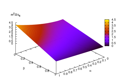
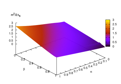
Figure 4: $m^{2}$ for the first two KK modes of the vector perturbation. When $\alpha=1$, the values correspond to $\mu_{(+)}^{2}$ for $n=1$ (left) and $\mu_{(-)}^{2}$ for $n=2$ (right). These are non-negative for the entire region of $(\alpha,\beta)$.

Fig. 4 shows $m^{2}$ for the first two KK modes of the vector perturbation. We find that $m^{2}$ is non-negative for the entire region of $(\alpha,\beta)$. Therefore, there are no unstable modes in the vector sector.

IV.3 Tensor perturbation

The tensor perturbation is given by

$$g_{MN}\mathrm{d}x^{M}\mathrm{d}x^{N} =r^{2}(g_{\mu\nu}+h_{(\mathrm{T})}T_{(\mathrm{T})\mu\nu})\mathrm{d}x^{\mu}\mathrm{d}x^{\nu}+\frac{\mathrm{d}r^{2}}{f}+f\mathrm{d}\phi^{2},$$ (61)

$$A_{M}\mathrm{d}x^{M} =A\mathrm{d}\phi,$$

where $T_{(\mathrm{T})\mu\nu}$ is the tensor harmonics on the 4D de Sitter space, which satisfies the transverse and traceless conditions, $\nabla^{\mu}T_{(\mathrm{T})\mu\nu}=T_{(\mathrm{T})}{}^{\mu}{}_{\mu}=0$, and

$$\nabla^{2}T_{(\mathrm{T})\mu\nu}-(m^{2}+2h^{2})T_{(\mathrm{T})\mu\nu}=0.$$ (62)

The perturbed Einstein equation becomes

$$\frac{1}{r^{2}}(r^{4}fh^{\prime}_{(\mathrm{T})})^{\prime}+m^{2}h_{(\mathrm{T})}=0,$$ (63)

and there is no relevant equation coming from the Maxwell equation. With the coordinate $w$, this is written as

$$\frac{1}{[(1-\alpha)w+(1+\alpha)]^{2}}\partial_{w}\left\{[(1-\alpha)w+(1+\alpha)]^{4}\bar{f}\partial_{w}h_{(\mathrm{T})}\right\}+2\mu^{2}h_{(\mathrm{T})}=0.$$ (64)

IV.3.1 Analytic solution for $\alpha=1$

For $\alpha=1$ the perturbation equation becomes

$$\partial_{w}[(1-w^{2})\partial_{w}h_{(\mathrm{T})}]+\frac{4\mu^{2}}{4-3\beta}h_{(\mathrm{T})}=0.$$ (65)

The regular solution is given by

$$h_{(\mathrm{T})}=P_{n}(w),$$ (66)

where $P_{n}$ is the Legendre function of the first kind. The KK mass squared $\mu^{2}$ is

$$\mu^{2}=\frac{4-3\beta}{4}n(n+1),$$ (67)

where $n=0,1,2,\cdots$. It is obvious that the lowest-mass mode is $n=0$ and it is massless, representing the 4D graviton.

IV.3.2 General $\alpha$

For the tensor perturbation it is clear that the zero mode is $h_{(\mathrm{T})}=\text{const.}$, i.e., a homogeneous mode.

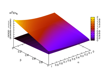
Figure 5: $m^{2}$ for the first KK mode of the tensor perturbation. The lower plane describes the particular mass, $m^{2}=9h^{2}/4$, for the tensor mode on the de Sitter space.

Fig. 5 shows $m^{2}$ for the first KK mode of the tensor perturbation. We find that $m^{2}$ for the KK modes is non-negative for the entire region of $(\alpha,\beta)$. Therefore, there is no unstable mode in the tensor sector. (See e.g. Hubeny:2002xn .)

V Summary and discussion

In this paper we have studied stability of the 6D braneworld solution with 4D de Sitter branes from two different perspectives.

One is thermodynamic stability of the braneworld solution. We have defined the de Sitter entropy in the six-dimensional braneworld by one quarter of the area of the cosmological horizon integrated over the extra dimensions. We have seen that this definition agrees with the $4$-dimensional de Sitter entropy defined on each brane. As shown in Fig. 1, the de Sitter entropy as a function of the conserved quantities $\eta$ and $\widehat{\Phi}$ is not single-valued but double-valued. Therefore, the de Sitter entropy divides the family of solutions into two branches, one with higher entropy (the high-entropy branch) and the other with lower entropy (the low-entropy branch), and defines the boundary between them (the critical curve).

The other is dynamical stability of the background solutions against linear perturbations. Perturbations are decomposed into the scalar-, vector- and tensor-sectors, according to the $4$-dimensional de Sitter symmetry, and we have calculated the lowest mass squared in each sector. We have found that when the Hubble expansion rate on the brane is larger than a critical value, there is a tachyonic mode in the scalar sector and thus the background is unstable. At the critical value, there appears a threshold massless mode in the scalar sector. On the other hand, there is no unstable mode in the vector- and tensor-sectors.

We have found that the critical value at which the threshold massless mode appears is exactly on the critical curve dividing the family of solutions into the high-entropy branch and the low-entropy branch. Therefore, we have shown that the low-entropy branch is dynamically unstable while the high-entropy branch is dynamically stable. Moreover, we have also seen that the $4$-dimensional effective Newton’s constant is positive in the high-entropy branch and negative in the low-entropy branch. In summary, we have shown the equivalence of the following three conditions:

• Thermodynamic stability.

• Dynamical stability.

• Positivity of the effective Newton’s constant.

The close connection between thermodynamic stability and dynamical stability has already been pointed out in the literature Braden:1990hw ; Maeda:1993ap ; Gubser:2000mm . The result of the present paper, thus, adds yet another example to the list of systems exhibiting the close connection between thermodynamic and dynamical properties. In the previous examples in the literature, however, one has to rely on numerical analysis to show the equivalence and the boundary between stable and unstable regions is not obtained rigorously. On the other hand, our system was simple enough to obtain the boundary analytically. In this sense, we may say that the analysis in the present paper is the first example in which the equivalence between thermodynamic stability and dynamical stability was proved. Moreover, we have shown that for our gravitational system the thermodynamic and dynamical properties of the spacetime is closely related to the sign of the effective Newton’s constant.

Non-linear evolution of the unstable solutions is one of the important subjects for the near future. While we have shown that the low-entropy branch is unstable, our analysis is limited by the linearized approximation and we do not know to what final state the spacetime will evolve from the low-entropy branch. A naive guess is that the system should evolve to the corresponding solution in the high-entropy branch with the same values of the conserved quantities, but there remains the possibility that the system might evolve towards a big crunch singularity or evolve to another unknown configuration Krishnan:2005su . Indeed, as seen from Fig. 1, for a solution in the low-entropy branch with a very large Hubble parameter close to the maximum value, there is no corresponding solution in the high-entropy branch. However, one can show that there is a solution with AdS branes for the same conserved quantities $\eta$ and $\widehat{\Phi}$. This indicates that the FRW cosmology on the brane in this regime should evolve towards a big crunch singularity unless there is another unknown stable solution without 4D maximal symmetry. It is worthwhile seeking such solutions without 4D maximal symmetry and also analyzing properties of solutions with AdS branes DeWolfe:2001nz . The whole phase structure including the high- and low-entropy branches, the AdS branch and possibly other new branches is unexplored.

Inclusion of general matter on the brane is also an interesting subject as a future work. In the present set-up, the 4D spacetime on the branes has the maximal symmetry and the stress energy tensor on the brane is restricted to the form of vacuum energy, or brane tension. It is certainly interesting to investigate dynamical stability and thermodynamic properties of the braneworld with more general Friedmann universe and matter contents on the brane. For this purpose, we need some extensions of the model to include arbitrary matter on the codimension-2 brane Peloso:2006cq ; Himmetoglu:2006nw ; Papantonopoulos:2006dv ; Kobayashi:2007kv . It is also interesting to consider supergravity extensions.

We expect that the close connection between thermodynamic stability and dynamical stability could be extended to models with branes of higher codimensions, i.e. models with more extra dimensions. We hope to investigate this subject in the future. Here, as the first step, let us briefly discuss extensions to models with more extra dimensions but without branes. We consider general Freund–Rubin flux compactifications with $\mathrm{dS}_{p}\times S^{q}$. The ($p+q$)-dimensional action is

$$I=\frac{1}{16\pi}\int\mathrm{d}^{p+q}x\sqrt{-g}\left(R-2\Lambda-\frac{1}{q!}F_{q}^{2}\right),$$ (68)

where $F_{q}$ is the $q$-form field for stabilizing the $q$-sphere. The metric and the $q$-form flux are given by

$$\mathrm{d}s^{2}=-\mathrm{d}t^{2}+e^{2ht}\mathrm{d}\vec{x}_{p-1}^{2}+\rho^{2}\mathrm{d}\Omega_{q}^{2},$$ (69)

and

$$F_{q}=b\epsilon_{\mu_{1}\cdots\mu_{q}},$$ (70)

where $\epsilon_{\mu_{1}\cdots\mu_{q}}$ is the volume element of the $q$-sphere. The Einstein and Maxwell equations reduce to two algebraic equations:

$$(q-1)\rho^{-2}-(p-1)h^{2} =b^{2},$$ (71)

$$(q-1)^{2}\rho^{-2}+(p-1)^{2}h^{2} =2\Lambda.$$

The entropy $S$ is given by

$$S=\frac{\Omega_{p-2}}{4h^{p-2}}\Omega_{q}\rho^{q}=-\frac{\Omega_{p-2}\Phi}{4h^{p-2}b},$$ (72)

where $\Phi$ is the total flux defined as $\Phi\equiv-b\rho^{q}\Omega_{q}$ and $\Omega_{p-2,q}$ are respectively the volume of the unit $(p-2)$-sphere and $q$-sphere. From (71) we can express $S$ as a function of one parameter. In this case we can also see that the entropy $S(\Phi)$ as a function of $\Phi$ is not single-valued and splits into a high-entropy branch and a low-entropy branch. The critical point dividing into two branches becomes

$$h^{2}_{\mathrm{cri}}=\frac{2\Lambda(p-2)}{(p-1)^{2}(p+q-2)},\quad b^{2}_{\mathrm{cri}}=\frac{(p-1)(p+q-2)}{(p-2)(q-1)}h^{2}_{\mathrm{cri}},$$ (73)

which is determined by $\mathrm{d}S/\mathrm{d}h=0$. These values are nothing but the threshold at which a tachyonic mode appears in the scalar sector Martin:2004wp . Therefore, we have shown the equivalence of thermodynamic stability and dynamical stability in the general Freund–Rubin flux compactifications with $\mathrm{dS}_{p}\times S^{q}$. It is worthwhile investigating a similar relation in models with branes of codimensions higher than two.

Appendix A Thermodynamic relations

In this appendix, we show the thermodynamic relations in the 6D braneworld solution with the 4D de Sitter space. The brane positions are determined by the two positive roots of $f(r)=0$, where

$$f(r)=h^{2}-\frac{\Lambda_{6}}{10}r^{2}-\frac{\mathcal{M}}{r^{3}}-\frac{b^{2}}{12r^{6}}.$$ (74)

Eliminating $\mathcal{M}$ from the conditions $f(1)=0$ and $f(\alpha)=0$, we obtain

$$h^{2}(1-\alpha^{3})-\frac{\Lambda_{6}}{10}(1-\alpha^{5})-\frac{b^{2}}{12\alpha^{3}}(\alpha^{3}-1)=0,$$ (75)

and this yields

$$\kappa_{+}+\kappa_{-}\alpha^{4} =-\frac{1}{2}f^{\prime}(1)+\frac{1}{2}f^{\prime}(\alpha)\alpha^{4}=\frac{\Lambda_{6}}{10}(1-\alpha^{5})-\frac{b^{2}}{4\alpha^{3}}(\alpha^{3}-1)$$ (76)

$$=h^{2}(1-\alpha^{3})-\frac{b^{2}}{3\alpha^{3}}(\alpha^{3}-1)$$

$$=\frac{3h^{4}}{4\pi}\mathcal{A}-b\Phi.$$

This is the relation between the total area of the horizon $\mathcal{A}$, the total magnetic flux of $U(1)$ field $\Phi$, and the proper periods at the brane positions $\kappa_{\pm}$ which are respectively defined as

$$\mathcal{A} =\Delta\phi\int_{\alpha}^{1}r^{2}\mathrm{d}r\frac{4\pi}{h^{2}}=\frac{4\pi}{3h^{2}}(1-\alpha^{3})\Delta\phi,$$ (77)

$$\Phi =\int F_{r\phi}\mathrm{d}r\wedge\mathrm{d}\phi=\frac{b}{3\alpha^{3}}(\alpha^{3}-1)\Delta\phi,$$

and

$$\kappa_{+}=-\frac{1}{2}f^{\prime}(1)\Delta\phi,\quad\kappa_{-}=\frac{1}{2}f^{\prime}(\alpha)\Delta\phi.$$ (78)

Here $\Delta\phi$ is a given period of the angular coordinate $\phi$ of extra dimensions. Recalling Eq. (4), we find $\kappa_{\pm}=2\pi-8\pi\sigma_{\pm}$ where $\sigma_{\pm}$ are tensions of the $r_{\pm}$-brane. We note that Eq. (76) is similar to the thermodynamic relation for the 6D RNdS black hole.

Furthermore we can obtain the differential relation for the above quantities which is similar to the first law of black hole mechanics. The parameters of this spacetime are determined by two equations, $f(1)=0$ and $f(\alpha)=0$; then the variation of parameters in the two equations becomes

$$f^{\prime}(\alpha)\mathrm{d}\alpha+2h\mathrm{d}h-\frac{\mathrm{d}\mathcal{M}}{\alpha^{3}}-\frac{b}{6\alpha^{6}}\mathrm{d}b =0,$$ (79)

$$2h\mathrm{d}h-\mathrm{d}\mathcal{M}-\frac{b}{6}\mathrm{d}b =0.$$

Eliminating $\mathrm{d}\mathcal{M}$, we have

$$\kappa_{-}\mathrm{d}\alpha^{4}-\mathcal{A}\mathrm{d}\left(\frac{3h^{4}}{4\pi}\right)+\Phi\mathrm{d}b=0.$$ (80)

Although the period of the angular coordinate, $\Delta\phi$, is necessary for determining the global geometry of the spacetime, locally it is irrelevant. In other words, $\mathcal{A}$, $\Phi$ and $\kappa_{\pm}$ in Eq. (76) are “extensive” quantities with respect to the normalization of $\Delta\phi$. Therefore we express the above relations in terms of following “intensive” quantities, $\eta\equiv\kappa_{+}/\kappa_{-}$, $\widehat{\mathcal{A}}\equiv\mathcal{A}/\kappa_{-}$, and $\widehat{\Phi}\equiv\Phi/\kappa_{-}$. Using these quantities normalized by $\kappa_{-}$ it is convenient to discuss the case with the tension of the $r_{-}$-brane fixed. From Eqs. (76) and (80), we have

$$\eta+\alpha^{4}=\frac{3h^{4}}{4\pi}\widehat{\mathcal{A}}-b\widehat{\Phi},$$ (81)

and

$$\mathrm{d}\alpha^{4}-\widehat{\mathcal{A}}\mathrm{d}\left(\frac{3h^{4}}{4\pi}\right)+\widehat{\Phi}\mathrm{d}b=0.$$ (82)

Combining these two equations we obtain another expression,

$$\mathrm{d}\eta=\frac{3h^{4}}{4\pi}\mathrm{d}\widehat{\mathcal{A}}-b\mathrm{d}\widehat{\Phi}.$$ (83)

When the tension of the $r_{-}$-brane is fixed, the variation of $\eta$ is directly related to the variation of the tension of the $r_{+}$-brane, i.e., $\mathrm{d}\eta=-\mathrm{d}\sigma_{+}$. In this sense the above expression is important.

Appendix B Euclidean action

In this appendix, we revisit the derivation of the thermodynamic relations from the Euclidean action. (See, for example, Braden:1990hw .) We take an ansatz for the Euclidean 6D metric with topology $S^{2}\times S^{4}$,

$$\mathrm{d}s^{2}=X(r)^{2}\mathrm{d}\phi^{2}+Y(r)^{2}\mathrm{d}r^{2}+r^{2}[(1-h^{2}\rho^{2})\mathrm{d}\tau^{2}+(1-h^{2}\rho^{2})^{-1}\mathrm{d}\rho^{2}+\rho^{2}\mathrm{d}\Omega^{2}],$$ (84)

and for the $U(1)$ field,

$$A_{M}\mathrm{d}x^{M}=A(r)\mathrm{d}\phi.$$ (85)

The 4-dimensional part of the metric is a 4-sphere with the radius $h$, which is the Euclidean continuation of the 4D de Sitter space with the Hubble parameter $h$ by the Wick rotation of the time coordinate $\tau\to i\tau$. The Euclidean time $\tau$ has a period $\Delta\tau=2\pi/h$ related with the de Sitter temperature.

We obtain a component of the Einstein tensor,

$$G^{\phi}{}_{\phi}=\frac{2}{r^{4}}\left[r^{3}\left(\frac{1}{Y^{2}}-h^{2}\right)\right]^{\prime},$$ (86)

and the non-vanishing components of the energy-momentum tensor are

$$T^{\phi}{}_{\phi}=T^{r}{}_{r}=-T^{\mu}{}_{\mu}=\frac{1}{2}\left(\frac{A^{\prime}}{XY}\right)^{2}.$$ (87)

The nontrivial Maxwell equation is

$$\left(\frac{r^{4}A^{\prime}}{XY}\right)^{\prime}=0,$$ (88)

which is integrated to yield

$$\frac{r^{4}A^{\prime}}{XY}=-b,$$ (89)

where $b$ is the integration constant.

The component of Einstein equation, $G^{\phi}{}_{\phi}-T^{\phi}{}_{\phi}+\Lambda_{6}=0$ is

$$\frac{2}{r^{4}}\left[r^{3}\left(\frac{1}{Y^{2}}-h^{2}\right)\right]^{\prime}+\Lambda_{6}-\frac{b^{2}}{2r^{8}}=0,$$ (90)

and it is easily integrated to obtain

$$\frac{1}{Y^{2}}=h^{2}-\frac{\Lambda_{6}}{10}r^{2}-\frac{b^{2}}{12r^{6}}-\frac{\mathcal{M}}{r^{3}},$$ (91)

where $\mathcal{M}$ is the integration constant. The Ricci scalar and the field strength are

$$R=-\frac{4}{r^{4}}\left[r^{3}\left(\frac{1}{Y^{2}}-h^{2}\right)\right]^{\prime}-\frac{2}{r^{4}XY}\left(\frac{r^{4}X^{\prime}}{Y}\right)^{\prime},$$ (92)

and

$$-\frac{1}{2}F_{MN}F^{MN}=-\left(\frac{A^{\prime}}{XY}\right)^{2}.$$ (93)

The Euclidean action is given by

$$I_{\mathrm{E}} =-\frac{1}{16\pi}\int\mathrm{d}^{6}x_{\mathrm{E}}\sqrt{g}\left(R-2\Lambda_{6}-\frac{1}{2}F_{MN}F^{MN}\right)$$ (94)

$$=-\frac{\Delta\phi}{16\pi}4\pi\beta\int_{0}^{1/h}\!\!\rho^{2}\mathrm{d}\rho\int_{\alpha}^{1}\mathrm{d}r\left\{-4XY\left[r^{3}\left(\frac{1}{Y^{2}}-h^{2}\right)\right]^{\prime}-2\left(\frac{r^{4}X^{\prime}}{Y}\right)^{\prime}-2\Lambda_{6}r^{4}XY-\frac{r^{4}A^{\prime 2}}{XY}\right\}$$

$$=-\frac{\Delta\phi\beta}{6h^{3}}\int_{\alpha}^{1}\mathrm{d}r\left\{bA^{\prime}-\left(\frac{r^{4}X^{\prime}}{Y}\right)^{\prime}\right\}$$

$$=-\frac{\beta}{6h^{3}}(b\Phi+\kappa_{+}+\alpha^{4}\kappa_{-}),$$

where

$$\left.\Delta\phi\frac{X^{\prime}}{Y}\right|_{r=\alpha}=\kappa_{+},\quad\left.\Delta\phi\frac{X^{\prime}}{Y}\right|_{r=1}=-\kappa_{-},$$ (95)

and

$$\Phi\equiv\Delta\phi(A|_{r=1}-A|_{r=\alpha}).$$ (96)

Note that $\kappa_{\pm}$ and $\Phi$ are the boundary data held fixed in the current action. Here, $\beta$ is the inverse of the temperature of the de Sitter horizon, i.e., $\beta\equiv\Delta\tau$.

Two 3-branes are located at $r=\alpha,1$, so we require

$$X(\alpha)=X(1)=0.$$ (97)

The regularities at $r=\alpha,1$ lead to $1/Y^{2}|_{r=\alpha,1}=0$, and we obtain

$$h^{2}-\frac{\Lambda_{6}}{10}\alpha^{2}-\frac{b^{2}}{12\alpha^{6}}-\frac{\mathcal{M}}{\alpha^{3}}=h^{2}-\frac{\Lambda_{6}}{10}-\frac{b^{2}}{12}-\mathcal{M}=0.$$ (98)

From these two conditions we can determine the two integration constants $b,\mathcal{M}$:

$$\mathcal{M}(\alpha,h)=(1+\alpha^{3})h^{2}-\frac{\Lambda_{6}(1-\alpha^{8})}{10(1-\alpha^{3})},\quad b^{2}(\alpha,h)=\frac{6\Lambda_{6}\alpha^{3}(1-\alpha^{5})}{5(1-\alpha^{3})}-12\alpha^{3}h^{2},$$ (99)

The reduced action $I^{*}$ for fixed $\kappa_{\pm}$ and $\Phi$ is

$$I^{*}(\Phi,\kappa_{+},\kappa_{-};\alpha,h)\equiv-\frac{\pi}{3h^{4}}(b\Phi+\kappa_{+}+\alpha^{4}\kappa_{-}).$$ (100)

Extremizing this action with respect to $\alpha$ and $h$ gives us

$$\frac{\partial I^{*}}{\partial\alpha} =-\frac{\pi}{3h^{4}}\left(\frac{\partial b}{\partial\alpha}\Phi+4\alpha^{3}\kappa_{-}\right)=0,$$ (101)

$$\frac{\partial I^{*}}{\partial h} =\frac{4\pi}{3h^{5}}(b\Phi+\kappa_{+}+\alpha^{4}\kappa_{-})-\frac{\pi}{3h^{4}}\frac{\partial b}{\partial h}\Phi=0.$$

These two conditions are reduced to

$$\Phi/\kappa_{-}=4\alpha^{3}\left(\frac{\partial b}{\partial\alpha}\right)^{-1},\quad\kappa_{+}+\kappa_{-}\alpha^{4}=\frac{3h^{4}}{\pi}S^{*}-b\Phi,$$ (102)

where $S^{*}$ is defined as

$$S^{*}(\Phi;\alpha,h)\equiv\frac{\pi\Phi}{12h^{3}}\frac{\partial b}{\partial h}=-\frac{\pi\alpha^{3}\Phi}{bh^{2}}.$$ (103)

We denote $(\alpha,h)$ satisfying the conditions (102) for given $\kappa_{\pm}$ and $\Phi$ as $\alpha_{\mathrm{e}}(\Phi,\kappa_{+},\kappa_{-})$ and $h_{\mathrm{e}}(\Phi,\kappa_{+},\kappa_{-})$, and we have a classical action

$$I[\Phi,\kappa_{+},\kappa_{-}] \equiv I^{*}(\Phi,\kappa_{+},\kappa_{-};\alpha_{\mathrm{e}},h_{\mathrm{e}})=-\frac{\pi}{3h_{\mathrm{e}}^{4}}(b_{\mathrm{e}}\Phi+\kappa_{+}+\alpha_{\mathrm{e}}^{4}\kappa_{-})$$ (104)

$$=-S^{*}(\Phi;\alpha_{\mathrm{e}},h_{\mathrm{e}})\equiv-S[\Phi,\kappa_{+},\kappa_{-}],$$

where $b_{\mathrm{e}}\equiv b(\alpha_{\mathrm{e}},h_{\mathrm{e}})$. Moreover, the differential relation is given by

$$\mathrm{d}S=-\mathrm{d}I=\frac{\pi}{3h_{\mathrm{e}}^{4}}(b_{\mathrm{e}}\mathrm{d}\Phi+\mathrm{d}\kappa_{+}+\alpha_{\mathrm{e}}^{4}\mathrm{d}\kappa_{-}),$$ (105)

or by using “intensive” variables $\widehat{S}$, $\widehat{\Phi}$ and $\eta$ we obtain the alternative expression

$$\mathrm{d}\widehat{S}=\frac{\pi}{3h^{4}}(b\mathrm{d}\widehat{\Phi}+\mathrm{d}\eta),\quad\eta+\alpha^{4}=\frac{3h^{4}}{\pi}\widehat{S}-b\widehat{\Phi}.$$ (106)

From the conditions (102) we obtain the stationary points of $I^{*}$, in other words, a series of classical equilibrium solutions. To see the (thermodynamic) stability of the solutions, we have to know which of the equilibrium solutions has the minimum of $I$ (or the maximum of $S$) for given $\Phi$ and $\kappa_{\pm}$. For example, requiring one of the conditions, $\partial I^{*}/\partial\alpha=0$, we regard $I^{*}$ as an one-parameter function of $h$. (Note that $\Phi$ and $\kappa_{\pm}$ are fixed.) Then, we have

$$\frac{\mathrm{d}I^{*}}{\mathrm{d}h} =\frac{\partial I^{*}}{\partial h}+\frac{\partial I^{*}}{\partial\alpha}\left(\frac{\partial\alpha}{\partial h}\right)_{\Phi,\kappa_{-}}=\frac{\partial I^{*}}{\partial h},$$ (107)

$$\frac{\mathrm{d}^{2}I^{*}}{\mathrm{d}h^{2}} =\frac{\partial^{2}I^{*}}{\partial h^{2}}+\frac{\partial^{2}I^{*}}{\partial h\partial\alpha}\left(\frac{\partial\alpha}{\partial h}\right)_{\Phi,\kappa_{-}}.$$

At a stationary point they become

$$\left.\frac{\mathrm{d}I^{*}}{\mathrm{d}h}\right|_{\alpha_{\mathrm{e}},h_{\mathrm{e}}} =0,$$ (108)

$$\left.\frac{\mathrm{d}^{2}I^{*}}{\mathrm{d}h^{2}}\right|_{\alpha_{\mathrm{e}},h_{\mathrm{e}}} =-\frac{4}{h}\left[\frac{\partial S^{*}}{\partial h}+\frac{\partial S^{*}}{\partial\alpha}\left(\frac{\partial\alpha}{\partial h}\right)_{\Phi,\kappa_{-}}\right]=-\frac{4}{h}\left(\frac{\partial S}{\partial h}\right)_{\Phi,\kappa_{-}}.$$

Hence, the condition for taking a minimum value of $I$ (a maximum value of $S$) for fixed $\Phi$ and $\kappa_{\pm}$ is given by

$$\left(\frac{\partial S}{\partial h}\right)_{\Phi,\kappa_{-}}<0.$$ (109)

Appendix C gauge choice

C.1 Harmonics on $\mathrm{dS}_{4}$

We give definitions of scalar, vector, and tensor harmonics on the 4D de Sitter space. $g_{\mu\nu}$ is the metric of the 4D de Sitter space with the Hubble parameter $h$, namely, $R_{\mu\nu\alpha\beta}=h^{2}[g_{\mu\alpha}g_{\nu\beta}-g_{\mu\beta}g_{\nu\alpha}]$, and $\nabla_{\mu}$ is the covariant derivative associated with $g_{\mu\nu}$.

The scalar harmonics $Y$ satisfies

$$\nabla^{2}Y=m^{2}Y.$$ (110)

The vector harmonics $V_{(\mathrm{T})\mu}$ satisfies

$$[\nabla^{2}-3h^{2}]V_{(\mathrm{T})\mu}=m^{2}V_{(\mathrm{T})\mu},\quad\nabla^{\mu}V_{(\mathrm{T})\mu}=0,$$ (111)

and $V_{(\mathrm{L})\mu}$ is defined as

$$V_{(\mathrm{L})\mu}=\partial_{\mu}Y.$$ (112)

The tensor harmonics $h_{(\mathrm{T})\mu\nu}$ satisfies

$$[\nabla^{2}-2h^{2}]T_{(\mathrm{T})\mu\nu}=m^{2}T_{(\mathrm{T})\mu\nu},\quad\nabla^{\mu}T_{(\mathrm{T})\mu\nu}=T_{(\mathrm{T})}{}^{\mu}{}_{\mu}=0,$$ (113)

and $T_{(\mathrm{TL,LL,Y})\mu\nu}$ is defined by

$$T_{(\mathrm{TL})\mu\nu} \equiv\nabla_{\mu}V_{(\mathrm{T})\nu}+\nabla_{\nu}V_{(\mathrm{T})\mu},$$ (114)

$$T_{(\mathrm{LL})\mu\nu} \equiv\nabla_{\mu}V_{(\mathrm{L})\nu}+\nabla_{\nu}V_{(\mathrm{L})\mu}-\frac{1}{2}g_{\mu\nu}\nabla^{\alpha}V_{(\mathrm{L})\alpha}$$

$$=2\nabla_{\mu}\nabla_{\nu}Y-\frac{m^{2}}{2}g_{\mu\nu}Y,$$

$$T_{(\mathrm{Y})\mu\nu} \equiv g_{\mu\nu}Y.$$

C.2 Gauge choice

We expand the perturbed metric in harmonics of the 4D de Sitter space with the Hubble parameter $h$ as

$$\delta g_{MN}\mathrm{d}x^{M}\mathrm{d}x^{N}= h_{ab}Y\mathrm{d}x^{a}\mathrm{d}x^{b}$$ (115)

$$+2(h_{(\mathrm{T})a}V_{(\mathrm{T})\mu}+h_{(\mathrm{L})a}V_{(\mathrm{L})\mu})\mathrm{d}x^{a}\mathrm{d}x^{\mu}$$

$$+(h_{(\mathrm{T})}T_{(\mathrm{T})\mu\nu}+h_{(\mathrm{TL})}T_{(\mathrm{TL})\mu\nu}+h_{(\mathrm{LL})}T_{(\mathrm{LL})\mu\nu}+h_{(\mathrm{Y})}T_{(\mathrm{Y})\mu\nu})\mathrm{d}x^{\mu}\mathrm{d}x^{\nu},$$

where $Y$, $V_{\mathrm{(T,L)}}$, and $T_{\mathrm{(T,TL,LL,Y)}}$ are scalar, vector, and tensor harmonics, respectively. Greek indices $\mu,\nu,\cdots$ run over the $4$D de Sitter space and Latin indices $a,b,\cdots$ run over the $2$D extra dimensions $(r,\phi)$. The coefficients $h_{ab}$, $h_{(\mathrm{T})a}$, $h_{(\mathrm{L})a}$, $h_{(\mathrm{T})}$, $h_{(\mathrm{TL})}$, $h_{(\mathrm{LL})}$, and $h_{(\mathrm{Y})}$ depend only on $r$ assuming that the perturbations are axisymmetric. The perturbations of the $U(1)$ gauge field can be expanded as

$$\delta A_{M}\mathrm{d}x^{M}=a_{a}Y\mathrm{d}x^{a}+(a_{(\mathrm{T})}V_{(\mathrm{T})\mu}+a_{(\mathrm{L})}V_{(\mathrm{L})\mu})\mathrm{d}x^{\mu},$$ (116)

The infinitesimal coordinate transformation and $U(1)$ gauge transformation are

$$\delta g_{MN}\to\delta g_{MN}-\mathcal{L}_{\xi}g_{MN},\quad\delta A_{M}\to\delta A_{M}+\partial_{M}\chi-\mathcal{L}_{\xi}A_{M}.$$ (117)

Also, the gauge parameters can be expanded as

$$\xi_{M}\mathrm{d}x^{M}=(\xi_{(\mathrm{T})}V_{(\mathrm{T})\mu}+\xi_{(\mathrm{L})}V_{(\mathrm{L})\mu})\mathrm{d}x^{\mu}+\xi_{a}Y\mathrm{d}x^{a},\quad\chi=\chi_{(\mathrm{Y})}Y.$$ (118)

The tensor-type component is gauge invariant:

$$h_{\mathrm{(T)}}\to\bar{h}_{\mathrm{(T)}}=h_{\mathrm{(T)}}.$$ (119)

The vector-type components transform as

$$h_{\mathrm{(TL)}} \to\bar{h}_{\mathrm{(TL)}}=h_{\mathrm{(TL)}}-\xi_{(\mathrm{T})}, h_{(\mathrm{T})r} \to\bar{h}_{(\mathrm{T})r}=h_{(\mathrm{T})r}-\xi^{\prime}_{(\mathrm{T})}+\frac{2}{r}\xi_{(\mathrm{T})},$$ (120)

$$h_{(\mathrm{T})\phi} \to\bar{h}_{(\mathrm{T})\phi}=h_{(\mathrm{T})\phi}, a_{(\mathrm{T})} \to\bar{a}_{(\mathrm{T})}=a_{(\mathrm{T})},$$

where the prime denotes the derivative with respect to $r$. Choosing $\xi_{(\mathrm{T})}=h_{\mathrm{(TL)}}$, we have $\bar{h}_{\mathrm{(TL)}}=0$. With this gauge choice we use new variables. Using a part of perturbed Einstein equation we obtain algebraically

$$h_{(\mathrm{T})r}=\frac{C}{r^{2}f},$$ (121)

where $C$ is an arbitrary constant for $m^{2}=-6h^{2}$, or $C=0$ for $m^{2}\neq-6h^{2}$. When $m^{2}=-6h^{2}$, this constant corresponds to the pure gauge mode for tensor perturbations because $\nabla^{\mu}T_{(\mathrm{TL})\mu\nu}=[\nabla^{2}+3h^{2}]V_{(\mathrm{T})\nu}=0$ and $T_{(\mathrm{TL})}{}^{\mu}{}_{\mu}=2\nabla^{\mu}V_{(\mathrm{T})\mu}=0$. Hence we can choose $C=0$.

The scalar-type components transform as

$$h_{(\mathrm{LL})} \to\bar{h}_{(\mathrm{LL})}=h_{(\mathrm{LL})}-\xi_{(\mathrm{L})}, h_{(\mathrm{Y})} \to\bar{h}_{(\mathrm{Y})}=h_{(\mathrm{Y})}-\frac{m^{2}}{2}\xi_{(\mathrm{L})}-2rf\xi_{r},$$ (122)

$$h_{(\mathrm{L})r} \to\bar{h}_{(\mathrm{L})r}=h_{(\mathrm{L})r}-\xi^{\prime}_{(\mathrm{L})}+\frac{2}{r}\xi_{(\mathrm{L})}-\xi_{r}, h_{(\mathrm{L})\phi} \to\bar{h}_{(\mathrm{L})\phi}=h_{(\mathrm{L})\phi}-\xi_{\phi},$$

$$h_{rr} \to\bar{h}_{rr}=h_{rr}-2\xi^{\prime}_{r}-\frac{f^{\prime}}{f}\xi_{r}, h_{r\phi} \to\bar{h}_{r\phi}=h_{r\phi}-\xi^{\prime}_{\phi}+\frac{f^{\prime}}{f}\xi_{\phi},$$

$$h_{\phi\phi} \to\bar{h}_{\phi\phi}=h_{\phi\phi}-ff^{\prime}\xi_{r}, a_{(\mathrm{L})} \to\bar{a}_{(\mathrm{L})}=a_{(\mathrm{L})}+\chi_{(\mathrm{Y})}-A\frac{\xi_{\phi}}{f},$$

$$a_{r} \to\bar{a}_{r}=a_{r}+\chi^{\prime}_{(\mathrm{Y})}-A\left(\frac{\xi_{\phi}}{f}\right)^{\prime}, a_{\phi} \to\bar{a}_{\phi}=a_{\phi}-A^{\prime}f\xi_{r}.$$

Choosing

$$\xi_{(\mathrm{L})} =h_{(\mathrm{LL})}, \xi_{r} =h_{(\mathrm{L})r}-h^{\prime}_{(\mathrm{LL})}+\frac{2}{r}h_{(\mathrm{LL})},$$ (123)

$$\xi_{\phi} =f\int^{r}_{C^{\prime}}\mathrm{d}\rho\frac{h_{r\phi}(\rho)}{f(\rho)}, \chi_{(\mathrm{Y})} =-a_{(\mathrm{L})}+A\frac{\xi_{\phi}}{f},$$

where $C^{\prime}$ is an arbitrary constant, we have $\bar{h}_{(\mathrm{LL})}=\bar{h}_{(\mathrm{L})r}=\bar{h}_{r\phi}=\bar{a}_{(\mathrm{L})}=0$. With this gauge choice we redefine each component as follows:

$$\bar{h}_{(\mathrm{Y})} \equiv\Psi, \bar{h}_{(\mathrm{L})\phi} \equiv h_{(\mathrm{L})\phi}, \bar{h}_{rr} \equiv(\Phi_{1}+\Phi_{2})/f,$$ (124)

$$\bar{h}_{\phi\phi} \equiv-(\Phi_{1}+3\Phi_{2})f, \bar{a}_{r} \equiv a_{r}, \bar{a}_{\phi} \equiv a_{\phi}.$$

Moreover, using parts of the perturbed Einstein and Maxwell equations we algebraically obtain the following relations for four variables:

$$\Psi=\Phi_{2},\quad h_{(\mathrm{L})\phi}=Cf,\quad a_{r}=-\frac{A^{\prime}}{f}h_{(\mathrm{L})\phi}=-CA^{\prime},\quad a_{\phi}=\frac{1}{A^{\prime}}\left[f^{\prime}\Phi_{2}+\frac{1}{2r^{2}}(fr^{2}\Phi_{1})^{\prime}\right],$$ (125)

where $C$ is an arbitrary constant for $m^{2}=0$, or $C=0$ for $m^{2}\neq 0$. This constant corresponds to the residual (homogeneous) gauge freedom, $\xi_{\phi}=Cf$ and $\chi_{(\mathrm{Y})}=CA$. We can set $C=0$, i.e., $h_{(\mathrm{L})\phi}=a_{r}=0$.

References

- (1) S. Mukohyama, Y. Sendouda, H. Yoshiguchi and S. Kinoshita, JCAP 0507, 013 (2005) [arXiv:hep-th/0506050].
- (2) H. Yoshiguchi, S. Mukohyama, Y. Sendouda and S. Kinoshita, JCAP 0603, 018 (2006) [arXiv:hep-th/0512212].
- (3) Y. Sendouda, S. Kinoshita and S. Mukohyama, Class. Quant. Grav. 23, 7199 (2006) [arXiv:hep-th/0607189].
- (4) A. V. Frolov and L. Kofman, Phys. Rev. D 69, 044021 (2004) [arXiv:hep-th/0309002].
- (5) C. R. Contaldi, L. Kofman and M. Peloso, JCAP 0408, 007 (2004) [arXiv:hep-th/0403270].
- (6) R. Bousso, O. DeWolfe and R. C. Myers, Found. Phys. 33, 297 (2003) [arXiv:hep-th/0205080].
- (7) J. U. Martin, JCAP 0504, 010 (2005) [arXiv:hep-th/0412111].
- (8) C. Krishnan, S. Paban and M. Zanic, JHEP 0505, 045 (2005) [arXiv:hep-th/0503025].
- (9) S. Mukohyama, arXiv:gr-qc/9812079.
- (10) H. W. Braden, J. D. Brown, B. F. Whiting and J. W. York, Phys. Rev. D 42, 3376 (1990).
- (11) K. I. Maeda, T. Tachizawa, T. Torii and T. Maki, Phys. Rev. Lett. 72, 450 (1994) [arXiv:gr-qc/9310015].
- (12) T. Prestidge, Phys. Rev. D 61, 084002 (2000) [arXiv:hep-th/9907163].
- (13) S. S. Gubser and I. Mitra, JHEP 0108, 018 (2001) [arXiv:hep-th/0011127].
- (14) S. S. Gubser and I. Mitra, arXiv:hep-th/0009126.
- (15) H. S. Reall, Phys. Rev. D 64, 044005 (2001) [arXiv:hep-th/0104071].
- (16) G. Arcioni and E. Lozano-Tellechea, Phys. Rev. D 72, 104021 (2005) [arXiv:hep-th/0412118].
- (17) T. Harmark, V. Niarchos and N. A. Obers, arXiv:hep-th/0701022.
- (18) G. W. Gibbons and S. W. Hawking, Phys. Rev. D 15, 2738 (1977).
- (19) A. Strominger, JHEP 0110, 034 (2001) [arXiv:hep-th/0106113].
- (20) R. Bousso, Rev. Mod. Phys. 74, 825 (2002) [arXiv:hep-th/0203101].
- (21) P. G. O. Freund and M. A. Rubin, Phys. Lett. B 97, 233 (1980).
- (22) S. M. Carroll and M. M. Guica, arXiv:hep-th/0302067.
- (23) J. Garriga and M. Porrati, JHEP 0408, 028 (2004) [arXiv:hep-th/0406158].
- (24) A. Higuchi, Nucl. Phys. B 282, 397 (1987).
- (25) S. Deser and A. Waldron, Phys. Lett. B 508, 347 (2001) [arXiv:hep-th/0103255].
- (26) T. Garidi, J. P. Gazeau and M. V. Takook, J. Math. Phys. 44, 3838 (2003) [arXiv:hep-th/0302022].
- (27) V. E. Hubeny and M. Rangamani, JHEP 0205, 027 (2002) [arXiv:hep-th/0202189].
- (28) O. DeWolfe, D. Z. Freedman, S. S. Gubser, G. T. Horowitz and I. Mitra, Phys. Rev. D 65, 064033 (2002) [arXiv:hep-th/0105047].
- (29) M. Peloso, L. Sorbo and G. Tasinato, Phys. Rev. D 73, 104025 (2006) [arXiv:hep-th/0603026].
- (30) B. Himmetoglu and M. Peloso, arXiv:hep-th/0612140.
- (31) E. Papantonopoulos, A. Papazoglou and V. Zamarias, arXiv:hep-th/0611311.
- (32) T. Kobayashi and M. Minamitsuji, arXiv:hep-th/0703029.