Abstract

We prove the universality of the Hernandez-Lopez phase by deriving it from first principles. We find a very simple integral representation for the phase and discuss its possible origin from a nested Bethe ansatz structure. Hopefully, the same kind of derivation could be used to constrain higher orders of the full quantum dressing factor.

1 Introduction

Bethe ansatz equations, first written by Bethe in the study of one dimensional metals [1], seem to be a key ingredient in the AdS/CFT duality [2] between $\mathcal{N}=4$ SYM and type IIB superstring theory on $AdS_{5}\times S^{5}$.

The $\mathcal{N}=4$ SYM dilatation operator in the planar limit can be perturbatively computed in powers of the t’Hooft coupling $\lambda$. In the seminal work of Minahan and Zarembo [3] it was shown that the $1$-loop dilatation operator acts on the six real scalars of the theory exactly like an integrable $SO(6)$ spin chain Hamiltonian. Restricting ourselves to two complex scalars we obtain the same Hamiltonian considered by Bethe for the Heisemberg spin chain. The eigenstates are $K$ magnon states with momentum and energy parameterized by the roots $u_{i}$ which satisfy Bethe equations

$$\left(\frac{u_{i}+i/2}{u_{i}-i/2}\right)^{L}=\prod_{j\neq i}^{K}\frac{u_{i}-u_{j}+i}{u_{i}-u_{j}-i}\,.$$

The full $\mathcal{N}=4$ $1$-loop dilatation operator [4] is also given by an integrable Hamiltonian whose spectrum is dictated by a system of seven Bethe equations [5], corresponding to the seven nodes of the $psu(2,2|4)$ Dynkin diagram. In [6] the all loop version of the Bethe equation for the $SU(2)$ sector was conjectured to be

$$\left(\frac{y^{+}_{j}}{y^{-}_{j}}\right)^{L}=\prod_{j\neq i}^{K}\frac{u_{i}-u_{j}+i}{u_{i}-u_{j}-i}\,,$$ (1)

where $y_{j}(u_{j})$ and $y_{j}^{\pm}(u_{j})$ are given by

$$y+\frac{1}{y}=\frac{4\pi}{\sqrt{\lambda}}\,u\,\,\,\,\,\,,\,\,\,\,\,\,y^{\pm}+\frac{1}{y^{\pm}}=\frac{4\pi}{\sqrt{\lambda}}\left(u\pm\frac{i}{2}\right)\,.$$

On the other hand, for the same sector but from the string side of the correspondence, a map between classical string solutions and Riemann surfaces was proposed [7]. The resemblance between the cuts connecting the different sheets of these Riemann surfaces and the distribution of roots of the Bethe equations in the scaling limit seemed to indicate that the former could be the continuous limit of some quantum string Bethe ansatz. In [8] these equations were proposed to be

$$\left(\frac{y^{+}_{j}}{y^{-}_{j}}\right)^{L}=\prod_{j\neq i}^{K}\frac{u_{i}-u_{j}+i}{u_{i}-u_{j}-i}\,\sigma_{\rm AFS}^{2}(u_{i},u_{j})\,,$$ (2)

where

$$\sigma_{{\rm AFS}}(u_{i},u_{j})=\frac{1-1/(y_{j}^{+}y_{i}^{-})}{1-1/(y_{j}^{-}y_{i}^{+})}\left(\frac{y_{j}^{-}y_{i}^{-}-1}{y_{j}^{-}y_{i}^{+}-1}\frac{y_{j}^{+}y_{i}^{+}-1}{y_{j}^{+}y_{i}^{-}-1}\right)^{i(u_{j}-u_{i})}\,.$$ (3)

The striking similarity between (1) and (2) naturally led to the proposal that both sides of the correspondence would be described by the same equation which a scalar factor $\sigma^{2}$ interpolating from $\sigma_{\rm AFS}^{2}$ for large t’Hooft coupling to $1$ for small $\lambda$.

In [9] Beisert and Staudacher (BS) conjectured the all-loop Bethe equations for the full $PSU(2,2|4)$ group and in [10] these equations were brought to firmer ground. As before, one of the main tools used to guess the form of these equations was the existence of the classical algebraic curve for the full superstring on $AdS_{5}\times S^{5}$ [20]. The seven equations for the seven types of roots $u_{a,j}$ are entangled and the middle equation, the most complicated one, can be written as

$$\left(\frac{y^{+}_{4,k}}{y^{-}_{4,k}}\right)^{L} = e^{-i{\cal V}(y_{4,k})}\prod_{j\neq k}^{K_{4}}\frac{u_{k,4}-u_{j,4}+i}{u_{k,4}-u_{j,4}-i}\,\sigma_{\rm AFS}^{2}(u_{4,k},u_{4,j})$$ (4)

$$\qquad\times\prod_{j=1}^{K_{1}}\frac{1-1/y_{4,k}^{-}y_{1,j}}{1-1/y_{4,k}^{+}y_{1,j}}\prod_{j=1}^{K_{3}}\frac{y_{4,k}^{-}-y_{3,j}}{y_{4,k}^{+}-y_{3,j}}\prod_{j=1}^{K_{5}}\frac{y_{4,k}^{-}-y_{5,j}}{y_{4,k}^{+}-y_{5,j}}\prod_{j=1}^{K_{7}}\frac{1-1/y_{4,k}^{-}y_{7,j}}{1-1/y_{4,k}^{+}y_{7,j}}\,.$$

Finally, the energy of the string states (or anomalous dimension of the SYM operators) is carried by the middle root only

$$\Delta=\frac{\sqrt{\lambda}}{2\pi}\sum_{i=1}^{K_{4}}\left(\frac{i}{y_{4,j}^{+}}-\frac{i}{y_{4,j}^{-}}\right)\ .$$ (5)

The potential phase $\mathcal{V}$ should be responsible for the interpolation between the YM and the string equations for small and large t’Hooft coupling $\lambda$.

Based on the $1$-loop shift analysis of some classical circular strings [11] Hernandez and Lopez proposed a universal form for the first $1/\sqrt{\lambda}$ correction in $\mathcal{V}$ [12] which should be able to reproduce, together with the finite size corrections to the scaling limit [13, 14], the $1$-loop shift around any classical solution. This was quite a bold proposal since it relied solely on the analysis of rank one rigid circular strings. In [15] the proposed phase passed a very nontrivial test – it was shown to reproduce the non-analytic contribution to the $1$-loop shift around a simple $SU(3)$ solution. However, at the present stage, only for the $sl(2)$ one cut solution the $1$-loop shift from the Bethe ansatz equations is completely understood [13, 12].

Recently, using the crossing constraint [16] and transcendentality principles [17], the full form of the scalar factor was conjectured from the string [18] and gauge [19] theory points of view.

It is therefore fair to say that the advance in the last four years was spectacular. On the other hand it is also true that there is a great deal of conjectures involved one should both check and, hopefully, proof (or disproof). In this article we establish rigourously the Hernandez-Lopez phase by fully proving its universality.

Finally we discuss a possible origin for this phase from a nested Bethe ansatz approach.

2 Brief derivation of the Hernandez-Lopez coefficients

One can compute the fluctuation energies, i.e. the energy level spacing in the spectrum of the string, around any classical string solution in $AdS_{5}\times S^{5}$. To do so one should first map the classical configuration to an $8$–sheet Riemann surface [20] described by a set of $8$ quasi-momenta $p_{i}(x)$. In particular the classical energy ${\cal E}_{cl}$ of the solution is encoded in the large $x$ asymptotics of the $p_{i}(x)$. Then, to compute the fluctuation energies ${\cal E}_{n}^{ij}$ one adds $N_{n}^{ij}$ poles with residue

$$\alpha(x)=\frac{\sqrt{\lambda}}{4\pi}\frac{x^{2}}{x^{2}-1}$$

to the quasi-momenta $p_{i}$ and $p_{j}$. The choice of the pairs of sheets $ij$ corresponds to the several string polarizations and the mode number $n$, the Fourier mode of the excitation, fixes the position $x_{n}$ of the new poles by [21]

$$p_{i}(x_{n})-p_{j}(x_{n})=2\pi n\,.$$ (6)

Then the excitation energies can be read from the large $x$ asymptotic of the perturbed quasi-momenta [21]

$${\cal E}={\cal E}_{cl}+\sum_{n=-\infty}^{\infty}\sum_{ij}N_{n}^{ij}{\cal E}_{n}^{ij}\,$$

An object of prime interest obtained from these fluctuation energies is the $1$-loop shift [22]

$${\cal E}_{0}=\frac{1}{2}\sum_{n=-\infty}^{\infty}\sum_{ij}(-1)^{F}{\cal E}_{n}^{ij}$$ (7)

where $(-1)^{F}=\pm 1$ for bosonic and fermionic excitations respectively. To sum over all fluctuation energies it is extremely useful to employ the technique used by Schafer-Nameki in [23] and integrate them in the $n$ plane using the poles of the cotangent to pick the integer values of the mode numbers $n$,

$${\cal E}_{0}=\frac{1}{4i}\int_{\mathcal{C}}\cot(\pi n)\left(\sum_{ij}(-1)^{F}{\cal E}_{n}^{ij}\right)dn$$ (8)

where $\mathcal{C}$ encircles all the poles of $\cot$ (and only them) . The structure of singularities of the fluctuation energies in the complex $n$ plane is intricate and we shall discuss it in more detail elsewhere [24]. For a simple $su(2)$ circular string solution this analysis was carried out in [23].

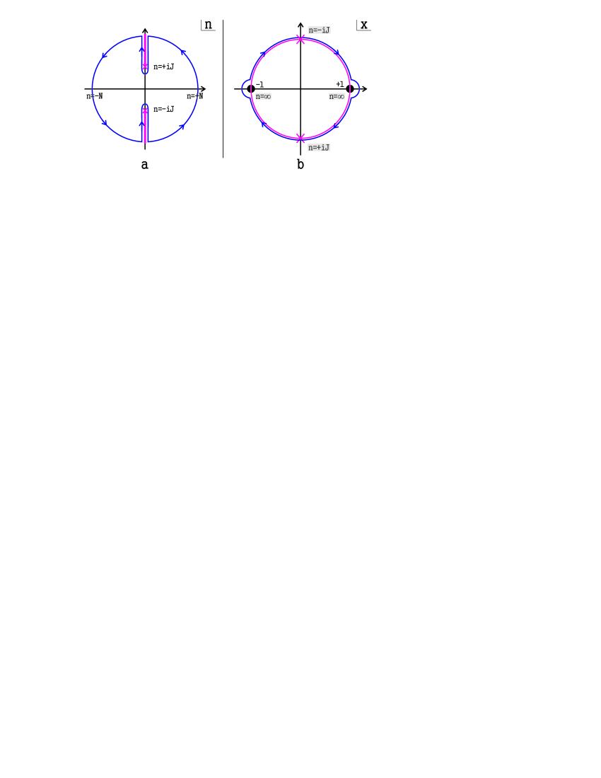
Figure 1: a. Analytical structure of the BMN frequencies $\sqrt{n^{2}+{\cal J}^{2}}$ and integration contour for (8). b. Same picture in the $x$ plane obtained through the map $\frac{x}{x^{2}-1}=\frac{n}{2{\cal J}}$. The branchpoints are mapped to $x=\pm i$. As $N\rightarrow\infty$ the integration path is mapped to the unit circle.

Let us consider the sum of the BMN frequencies [25] $\sqrt{n^{2}+{\cal J}^{2}}$ from $n=-N$ to $n=N$ with $N$ large. In the $n$ plane, for each frequency, the integral (8) over $n$ can be deformed to run along the cuts in the imaginary $n$ axis with branchpoints $n=\pm i{\cal J}$ as depicted in figure 1a. Moreover, for large ${\cal J}$, we can replace the $\cot$ in (8) by $\pm i$ for the lower/upper half plane. Through (6) we can map the integration contour to the $x$ plane. For this solution the quasi-momenta are very simple and

$$p_{i}-p_{j}=\frac{4\pi{\cal J}x}{x^{2}-1}$$

so that the branchcuts in the $n$ plane are mapped to the unit circle with the branchpoints $n=\pm i{\cal J}$ sent to $x=\mp i$ – see figure 1b . The integration contour for large $N$ is mapped to the solid (blue) contour in figure 1b and tends to the unit circle as $N\to\infty$.

For general classical solutions the picture is similar. For large $n$ the fluctuation frequencies should behave like $\sqrt{n^{2}}$ so that we will always have two branchpoints like as figure $1a$. These branchpoints are always large if the classical solution has some large global charge [24]. As before, when computing the integral along these branchcuts we can replace $\cot(\pi n)\to\mp i\,{\rm sign}({\rm Im}(n))$ with exponential precision. Let us call this contribution by $I_{phase}$ – the solid (blue) contour in figure 2a. Generically, contrary to what happened in the previous example, this is not the end of the story. There could be additional cuts in the $n$ plane whose contribution we have to subtract in order to pick the poles in $\cot$ (and only these poles) in (8). We denote the contribution from these integrals over the new cuts in the $n$ plane by $I_{anomaly}$ – the dashed (blue) contours in figure 2a. For the simple solutions considered in the literature these two terms usually bear the names of non-analytic and analytic contributions.

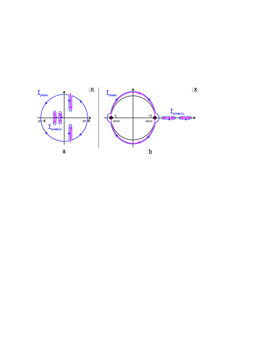
Figure 2: a. Typical analytical structure of the excitation energies as a function of the mode number $n$. The branchpoints associated to the cuts going to infinity are large if some charge of the classical solution is large. There could also be extra cuts in the $n$ plane. The integral (8) can be then split into two contributions $I_{phase}$ and $I_{anomaly}$ as depicted in the figure. b. The contour $I_{phase}$ going along the large cuts in the $n$ plane is mapped into some ellipsoidal form in the $x$ plane. The contours around the extra cuts in the $n$ plane are mapped to the cycles around the cuts of the classical solution around which we are quantizing.

The large branchcuts in the $n$ plane will then be mapped to some ellipsoidal curve in the $x$ plane passing through $x=\pm 1$ whereas the integrals around the extra cuts in the $n$ plane are mapped precisely to the integrals over the cuts of the original classical solution [24] – see figure 2b. Finally, to pass from an integral over the $n$ plane to an integral in the $x$ plane we just need to use the map (6),

$$dn=\frac{p_{i}^{\prime}-p_{j}^{\prime}}{2\pi}\,dx_{n}\,,$$ (9)

so that we see the typical $p^{\prime}$ and $\cot(\pi p)$ which always appear in the finite size correction analysis [13, 14]! We will study the general finite size corrections in a forthcoming publication [24] and elucidate its relation to $I_{anomaly}$. In this paper we prove the universality of the Hernandez-Lopez (HL) scalar factor by analyzing the $I_{phase}$ contribution around any classical configuration.

As we will see in the following section, the addition of the dressing factor $e^{i\cal V}$ in the middle equation (4) amounts to adding the potential to each quasimomenta $p_{i}\to p_{i}\pm{\cal V}/2$. Having this in mind, let us give a sketch of the proof. As we mentioned in the beginning of this section, by adding

$$\frac{\alpha(x)}{x-x_{n}^{ij}}$$

to the quasi-momenta $p_{i}$ and $p_{j}$ with $x_{n}^{ij}$ fixed by (6) we are considering a quantum fluctuation with mode number $n$ and polarization $ij$. Then, if we want to get the contribution $I_{phase}$ we should integrate this pole over $n$ using (9) and sum over the different polarizations with the appropriate signs (8). For example for $\tilde{p}_{1}$ we have $(i,j)=(\tilde{1},\tilde{3}),(\tilde{1},\tilde{4})$ bosonic excitation coming with a plus sign and $(i,j)=(\tilde{1},\hat{3}),(\tilde{1},\hat{4})$ for the fermionic excitations summed with a minus sign – see figure 3. Then we find that the contribution we must add for each $p_{i}$ is the same and reads

$${\cal V}(x)=\int_{-1}^{+1}\left[\tilde{p}_{3}^{\prime}+\tilde{p}_{4}^{\prime}-\hat{p}_{3}^{\prime}-\hat{p}_{4}^{\prime}\right]\left(\frac{\alpha(x)}{x-y}-\frac{\alpha(1/x)}{1/x-y}\right)\frac{dy}{2\pi}\,.$$ (10)

It is interesting to see that this potential is explicitly $x\to 1/x$ odd,

$${\cal V}(x)=-{\cal V}(1/x)\,.$$ (11)

Finally, as we will see in the next section, the combination of quasi-momenta appearing in (10) is precisely the one from which one reads the global charges $Q_{n}$,

$$\tilde{p}_{3}^{\prime}+\tilde{p}_{4}^{\prime}-\hat{p}_{3}^{\prime}-\hat{p}_{4}^{\prime}=\partial_{y}\left[G_{4}(y)-G_{4}(1/y)\right]\,.$$ (12)

where

$$G_{4}(y)=-\sum_{n=0}^{\infty}Q_{n+1}y^{n}\,,$$ (13)

so that we can expand the denominators in (10) for large $x$ and obtain

$${\cal V}(x)=\alpha(x)\!\!\!\!\!\sum_{\scriptsize\begin{array}[]{c}r,s=2\\ r\!+\!s\in Odd\end{array}}^{\infty}\!\!\!\!\frac{1}{\pi}\frac{(r-1)(s-1)}{(s-r)(r+s-2)}\left(\frac{Q_{r}}{x^{s}}-\frac{Q_{s}}{x^{r}}\right)$$ (14)

where we recognize precisely the Hernandez-Lopez coefficients! To obtain the values of the potential for $|x|<1$ we can simply use the exact symmetry (11) which is not manifest in the form (14). In the next section we shall explain the tight relation between this potential $\mathcal{V}$ and the BS equations and provide a detailed derivation of the scalar factor.

3 Constraining the scalar factor

In this section we shall fill the gaps in the sketchy derivation above. First we will start by explaining the relation between the quasi-momenta and the Beisert-Staudacher (BS) equations in the large $\lambda$ limit. We will see that relation (12) follows immediately from the definition of the quasi-momenta and that the phase $\mathcal{V}(x)$ appearing in (4) is simply translated into a potential for the quasi-momenta $p_{i}\to p_{i}\pm\mathcal{V}/2$. Then, we clarify the steps leading to (10), preform the large $N$ limit more carefully.

3.1 Classical limit

One of the main ingredients in the construction of the BS equations was the requirement that these equations reproduce the classical algebraical curve of [20]. For the sake of completeness, let us we make the passage to the classical limit explicit and at the same time introduce some important notations.

The seven BS equations, one for each node of a super Dynkin diagram of the $psu(2,2|4)$ algebra, give us the position of the roots $u_{a,j}$ where $a=1,\dots,7$ denotes the Dynkin node and $j=1,\dots,K_{a}$. The equation associated to the middle node of the Dynkin diagram takes the form (4). In fact, for a given number of roots, the Bethe equations have several solutions. To classify them one takes the log of the Bethe equation associated with each root. The different choices of the branch of the log correspond to the different solutions. In other words, to each root $u_{a,j}$ one should associate a mode number $n_{a,j}$. Thus, a choice of mode numbers amounts to fixing the quantum state.

To study the large $\lambda$ scaling limit,

$$u_{j}\sim L\sim K_{i}\sim\sqrt{\lambda}\,,$$ (15)

of the BS equations it is useful to introduce $8$ functions $\{\hat{p}_{1},\hat{p}_{2},\hat{p}_{3},\hat{p}_{4},\tilde{p}_{1},\tilde{p}_{2},\tilde{p}_{3},\tilde{p}_{4}\}$. First we define the resolvents $G_{a}$ and $H_{a}$ for each type of roots

$$G_{a}(x)=\sum_{j=1}^{K_{a}}\frac{\alpha(y_{a,j})}{x-y_{a,j}}\,\,,\,\,H_{a}(x)=\sum_{j=1}^{K_{a}}\frac{\alpha(x)}{x-y_{a,j}}\,.$$ (16)

Then, denoting $\bar{H}_{a}(x)=H_{a}(1/x)$ and ${\cal J}=L/\sqrt{\lambda}$, we have

$$\begin{array}[]{l|l}\!\hat{p}_{1}\!=\!+\displaystyle{\frac{2\pi{\cal J}x-G^{\prime}_{4}(0)x}{x^{2}-1}}\!-\!H_{1}\!+\!H_{2}\!+\!\bar{H}_{2}\!-\!\bar{H}_{3}\!+\!\frac{1}{2}{\cal V}&\tilde{p}_{1}\!=\!+\displaystyle{\frac{2\pi{\cal J}x+G_{4}(0)}{x^{2}-1}}\!-\!H_{1}\!-\!\bar{H}_{3}\!+\!\bar{H}_{4}\!+\!\frac{1}{2}\cal V{\color[rgb]{1,1,1}\frac{\frac{1}{2}}{\frac{1}{2}}}\\ \!\hat{p}_{2}\!=\!+\displaystyle{\frac{2\pi{\cal J}x-G^{\prime}_{4}(0)x}{x^{2}-1}}\!-\!H_{2}\!+\!H_{3}\!+\!\bar{H}_{1}\!-\!\bar{H}_{2}\!+\!\frac{1}{2}\cal V&\tilde{p}_{2}\!=\!+\displaystyle{\frac{2\pi{\cal J}x+G_{4}(0)}{x^{2}-1}}\!+\!H_{3}\!-\!H_{4}\!+\!\bar{H}_{1}\!+\!\frac{1}{2}\cal V{\color[rgb]{1,1,1}\frac{\frac{1}{2}}{\frac{1}{2}}}\\ \!\hat{p}_{3}\!=\!-\displaystyle{\frac{2\pi{\cal J}x-G^{\prime}_{4}(0)x}{x^{2}-1}}\!-\!H_{5}\!+\!H_{6}\!+\!\bar{H}_{6}\!-\!\bar{H}_{7}\!-\!\frac{1}{2}\cal V&\tilde{p}_{3}\!=\!-\displaystyle{\frac{2\pi{\cal J}x+G_{4}(0)}{x^{2}-1}}\!-\!H_{5}\!+\!H_{4}\!-\!\bar{H}_{7}\!-\!\frac{1}{2}\cal V{\color[rgb]{1,1,1}\frac{\frac{1}{2}}{\frac{1}{2}}}\\ \!\hat{p}_{4}\!=\!-\displaystyle{\frac{2\pi{\cal J}x-G^{\prime}_{4}(0)x}{x^{2}-1}}\!-\!H_{6}\!+\!H_{7}\!+\!\bar{H}_{5}\!-\!\bar{H}_{6}\!-\!\frac{1}{2}\cal V&\tilde{p}_{4}\!=\!-\displaystyle{\frac{2\pi{\cal J}x+G_{4}(0)}{x^{2}-1}}\!+\!H_{7}\!+\!\bar{H}_{5}\!-\!\bar{H}_{4}\!-\!\frac{1}{2}\cal V\end{array}$$ (21)

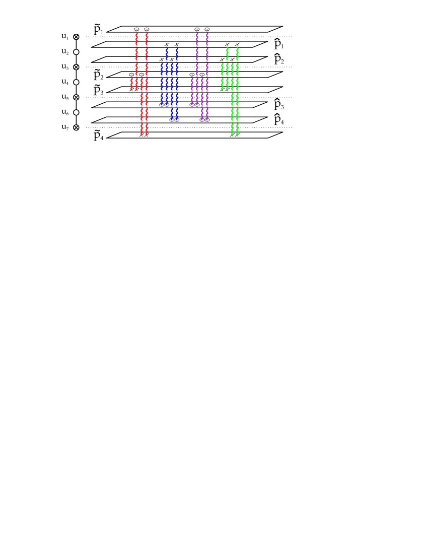
Figure 3: The 16 elementary physical excitations are the stacks (bound states) containing the middle node root. From the left to the right we have four $S^{5}$ fluctuations, four $AdS_{5}$ modes and eight fermionic excitations. The bosonic (fermionic) stacks contain an even (odd) number of fermionic roots signaled by a cross in the Dynkin diagram of $psu(2,2|4)$ in the left.

In the continuous limit, with a large number of roots for each mode number, roots with the same $n_{a,j}$ will condense into square root cuts. Moreover roots belonging to consecutive nodes of the Dynkin diagram can form bound states and in this way give rise to a cut $\mathcal{C}_{ij}$ connecting non-consecutive Dynkin nodes. As mentioned in the introduction only the middle roots $u_{4}$ carry energy (5). Then the 16 elementary physical excitations are the bound states represented in figure 1, each bound state corresponding to a different string polarization. These bound states, named stacks, were first found in [27] – we refer to this article for more details. We denote the values of a function $p(x)$ above and below some of these cuts $\mathcal{C}_{ij}$ by $p^{\pm}$. Then, in the large $\lambda$ limit, we can recast the seven BS equations as

$$p_{i}^{+}-p_{j}^{-}=2\pi n_{ij}\,\,,\,\,x\in\mathcal{C}_{ij}\,.$$ (22)

From the definition of the quasi-momenta we can read the large and small $x$ asymptotics, the behavior at the $x=\pm 1$ poles and understand how the several quasimomenta are related by the $x$ to $1/x$ inversion symmetry. To analyze the classical limit, moreover, we can drop the potential $\mathcal{V}$ whose contribution is of order $1/\sqrt{\lambda}$. We conclude that the analytical properties of $p$, together with the equations just mentioned are exactly the same as those of the quasimomenta defining the 8-sheet Riemann surface of Beisert, Kazakov, Sakai and Zarembo [20]. Thus, the classical limit coincides with this continuous limit.

3.2 Deriving the Hernandez-Lopez scalar factor

Until the end of this section we drop the phase $\mathcal{V}$ in the BS equations (and thus also in (21)). If we add a stack connecting sheets $i$ and $j$ to some configuration of Bethe roots with all roots condensed into some cuts as described above, the position of the new stack will be given by (6) and and all the other roots will be slightly shifted $u_{j}\rightarrow\tilde{u}_{j}$. Then the energy of the new configuration is given by the energy of the original configuration plus the fluctuation energy with mode number $n$ associated to the corresponding string polarization [21]

$$\tilde{\Delta}=\Delta+{\cal E}_{n}^{ij}\,.$$ (23)

Let us now perform a simple rewriting exercise and treat each of the roots of this new stack separately in $p_{k}$. That is, if the stack contains a root associated with the Dynkin node $a$ we write

$$G_{a}(x)\rightarrow G_{a}(x)+\frac{\alpha(x_{n})}{x-x_{n}}\,\,,\,\,H_{a}(x)\to H_{a}(x)+\frac{\alpha(x)}{x-x_{n}}$$

where $G_{a}$ and $H_{a}$ are now defined with the sum over roots going only over $a=1,\dots,K_{a}$ where $K_{a}$ is the original number of roots of type $u_{a,j}$. Then, with this new stack, each quasi-momentum $p_{k}$ can be written as before but using the new resolvents $G_{a}$ and $H_{a}$ containing only the $K_{a}$ original roots plus an extra term $V_{k}^{ij}$ which we call potential and read

$$\left(\begin{array}[]{c}V_{\hat{1}}(x)\\ V_{\hat{2}}(x)\\ V_{\hat{3}}(x)\\ V_{\hat{4}}(x)\end{array}\right)^{ij}=\left(\begin{array}[]{c}+1\\ +1\\ -1\\ -1\end{array}\right)\frac{x}{x^{2}-1}\frac{\alpha(x_{n}^{ij})}{(x_{n}^{ij})^{2}}+\left(\begin{array}[]{c}+\delta_{\hat{1}i}\\ +\delta_{\hat{2}i}\\ -\delta_{\hat{3}j}\\ -\delta_{\hat{4}j}\\ \end{array}\right)\frac{\alpha(x)}{x-x_{n}^{ij}}-\left(\begin{array}[]{c}+\delta_{\hat{2}i}\\ +\delta_{\hat{1}i}\\ -\delta_{\hat{4}j}\\ -\delta_{\hat{3}j}\\ \end{array}\right)\frac{\alpha(1/x)}{1/x-x_{n}^{ij}}\,,$$ (24)

and

$$\left(\begin{array}[]{c}V_{\tilde{1}}(x)\\ V_{\tilde{2}}(x)\\ V_{\tilde{3}}(x)\\ V_{\tilde{4}}(x)\end{array}\right)^{ij}=\left(\begin{array}[]{c}-1\\ -1\\ +1\\ +1\end{array}\right)\frac{1}{x^{2}-1}\frac{\alpha(x_{n}^{ij})}{x^{ij}_{n}}-\left(\begin{array}[]{c}+\delta_{\tilde{1}i}\\ +\delta_{\tilde{2}i}\\ -\delta_{\tilde{3}j}\\ -\delta_{\tilde{4}j}\\ \end{array}\right)\frac{\alpha(x)}{x-x_{n}^{ij}}+\left(\begin{array}[]{c}+\delta_{\tilde{2}i}\\ +\delta_{\tilde{1}i}\\ -\delta_{\tilde{4}j}\\ -\delta_{\tilde{3}j}\\ \end{array}\right)\frac{\alpha(1/x)}{1/x-x_{n}^{ij}}\,,$$ (25)

In (21) we saw that the inclusion of the phase $\mathcal{V}$ in the middle node of the BS equations amounts to adding the same potential $\cal V$ to all quasi-momenta. The main difference to what we have there is that now the $x_{n}$ roots hidden in the potential also contribute to the charges (because every stack contains a $u_{4}$ root)

$$Q_{m}=\oint\frac{dx}{2\pi i}\,\frac{G_{4}(x)}{x^{m}}+\frac{\alpha(x_{n})}{x_{n}^{m}}\,.$$ (26)

Moreover the potentials $V_{k}^{ij}$ are different for different quasi-momenta.

Suppose that instead of (23) we want

$$\tilde{\Delta}=\Delta+I_{phase}$$ (27)

with

$$I_{phase}\equiv\frac{1}{2}\lim_{N\to\infty}\int\limits_{-N}^{N}\sum_{ij}(-1)^{F}{\cal E}^{ij}_{n}dn$$ (28)

where the contour in the $n$ plane is as depicted in figure 4a. Then, by linearity, we need only to replace $V_{k}^{ij}$ by

$$V_{k}(x)=\frac{1}{2}\lim_{N\to\infty}\sum_{ij}\int\limits_{-N}^{N}(-1)^{F}V_{k}^{ij}(x,x^{ij}_{n})dn\ .$$ (29)

Let us now show that all the potentials $V_{k}$ are the same up to a sign and are equal to $\cal V$ (10) from the previous section. Indeed

1. For each summand in (29) we can pass to the $x$ plane through (9). As we explain in Appendix A we can assume that for all fluctuation energies the corresponding integral in the $x$ plane is the same and goes over the upper and lower halves of the circle of radius $1+\epsilon$ centered at the origin as plotted in figure 4b.

   

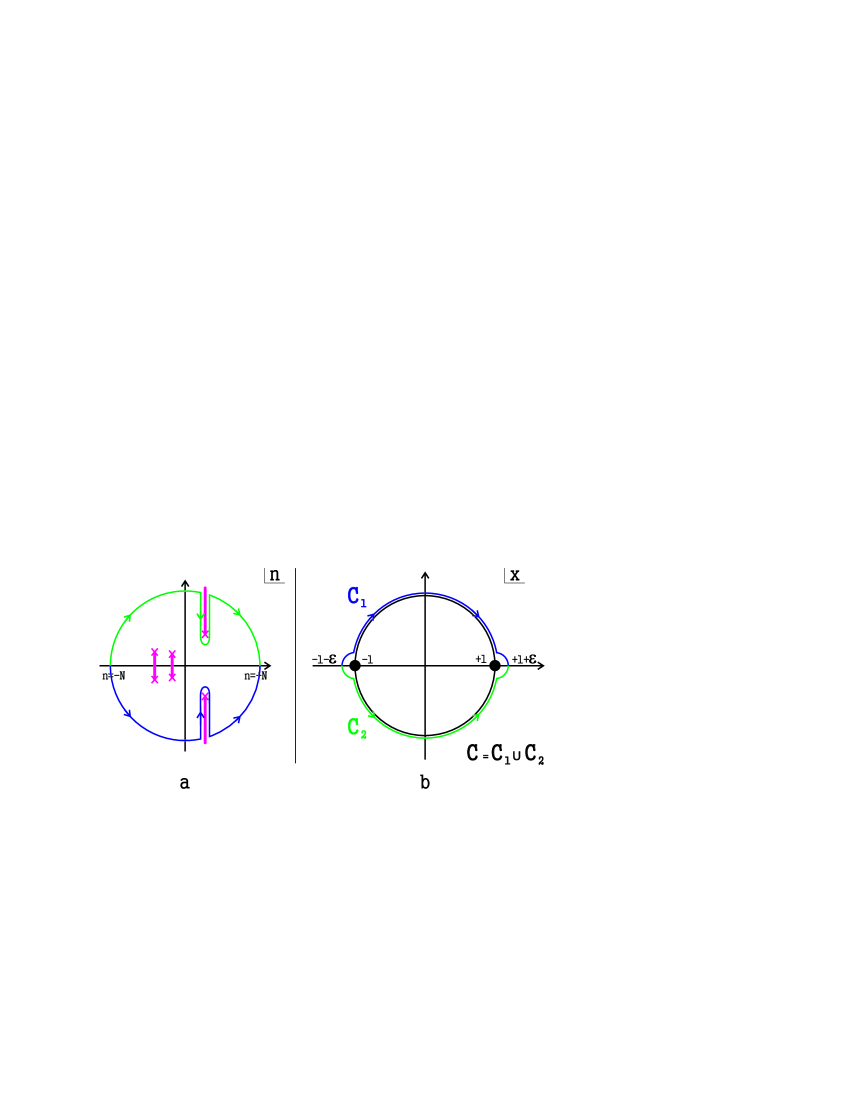
   Figure 4: a. The “non-analytic” contribution $I_{phase}$ is given by the integral (28) whose integration path goes along the large cuts discussed in section 2. The difference in orientations with respect to figure 2a is due to the absence of $\cot$ in expression (28) compared to (8). b. In the $x$ plane the integral can safely be deformed to go over the upper and lower halves of the unit circle. In the main text we use the shorthand $\int_{-1}^{+1}$ to denote $\frac{1}{2}\int_{C_{1}}+\frac{1}{2}\int_{C_{2}}$. The relation between the large $N$ regularization in the $n$ plane and the $\epsilon$ regularization in the $x$ plane is discussed in appendix A.

2. The first terms in (24) and (25) do not contribute to $V_{k}$. Indeed, if we integrate some function of $x_{n}^{ij}$ summed over the $16$ possible excitations listed in figure 3 with a $(-1)^{F}$ weight

   $$\sum_{ij}(-1)^{F}\int_{-N}^{N}f(x_{n}^{ij})dn$$

   we obtain, using (9),

   $$\int_{-1-\epsilon}^{+1+\epsilon}f(y)\left[\sum_{i=1,2\,,j=3,4}(\tilde{p}^{\prime}_{i}-\tilde{p}^{\prime}_{j})+(\hat{p}^{\prime}_{i}-\hat{p}^{\prime}_{j})-(\tilde{p}^{\prime}_{i}-\hat{p}^{\prime}_{j})-(\hat{p}^{\prime}_{i}-\tilde{p}^{\prime}_{j})\right]\frac{dy}{2\pi}=0\,.$$ (30)

3. Finally, consider for example $V_{\hat{1}}$. We have

   $$V_{\hat{1}}(x) = \frac{1}{2}\int_{-1-\epsilon}^{1+\epsilon}\left[(\hat{p}_{1}^{\prime}-\hat{p}_{3}^{\prime})+(\hat{p}_{1}^{\prime}-\hat{p}_{4}^{\prime})-(\hat{p}_{1}^{\prime}-\tilde{p}_{3}^{\prime})-(\hat{p}_{1}^{\prime}-\tilde{p}_{4}^{\prime})\right]\frac{\alpha(x)}{x-y}\frac{dy}{2\pi}$$

   $$- \frac{1}{2}\int_{-1-\epsilon}^{1+\epsilon}\left[(\hat{p}_{2}^{\prime}-\hat{p}_{3}^{\prime})+(\hat{p}_{2}^{\prime}-\hat{p}_{4}^{\prime})-(\hat{p}_{2}^{\prime}-\tilde{p}_{3}^{\prime})-(\hat{p}_{2}^{\prime}-\tilde{p}_{4}^{\prime})\right]\frac{\alpha(1/x)}{1/x-y}\frac{dy}{2\pi}\ .$$

   We see that $\hat{p}_{1}$ and $\hat{p}_{2}$ drop out so that the expression simplifies considerably. The same happens for the other $V_{i}$ and moreover, due to the super-tracelessness of the monodromy matrix, $\tilde{p}_{1}+\tilde{p}_{1}+\tilde{p}_{1}+\tilde{p}_{4}=\hat{p}_{1}+\hat{p}_{1}+\hat{p}_{1}+\hat{p}_{4}$, and all the potentials are equal. Using (12) we have

   $$V_{\hat{1},\hat{2},\tilde{1},\tilde{2}}(x)=-V_{\hat{3},\hat{4},\tilde{3},\tilde{4}}(x)\equiv{\cal V}(x)=\int_{-1}^{1}\partial_{y}\left[G_{4}(y)-G_{4}(1/y)\right]\left(\frac{\alpha(x)}{x-y}-\frac{\alpha(1/x)}{1/x-y}\right)\frac{dy}{2\pi}\,.$$ (31)

Notice also that due to 3) the extra terms in the charges (26) give no contribution! Thus, since now all potentials $V_{k}$ are equal to $\cal V$, we proved that for arbitrary configuration of Bethe roots, the addition of the Hernandez-Lopez phase will lead to an energy shift given by $I_{phase}$.

As we saw in the previous section, to obtain the Hernandez-Lopez phase as usually written in terms of charges it suffices to use (13). If we want, on the other hand, to write

$$e^{i\mathcal{V}(y_{4,k})}=\prod\limits_{j\neq k}^{K_{4}}e^{i\theta(y_{4,k},y_{4,j})}$$

where the factorized scattering property is manifest we just need to use the definition (16) and integrate over $y$ to get

$$\theta(x,y)=-\frac{\alpha(x)\,\alpha(y)}{\pi}\left[\left(\frac{1}{(x-y)^{2}}+\frac{1}{(xy-1)^{2}}\right)\log\left(\frac{x+1}{x-1}\frac{y-1}{y+1}\right)+\frac{2}{(x-y)(xy-1)}\right]$$ (32)

The real scattering phase, the phase that describes the scattering between two magnons in the Bethe ansatz equation, must inherit the explicit $x$ to $1/x$ oddness (11) of the potential. To obtain the values of the phase for $|x|<1$ we use $\theta(1/x,y)=-\theta(x,y)$. Alternatively, we recall that the contour in figure $4b$ tells us that to be completely rigorous we should replace the $\log$ in (32) by $\frac{1}{2}\left(\log_{+}(\dots)+\log_{-}(\dots)\right)$ where $\log_{\pm}$ has a branchcut in the upper/lower half of the unit circle – see figure 4b. Then the expression for $\theta(x,y)$ becomes explicitly $x$ to $1/x$ odd and is discontinuous on the unit circle. If, on the other hand, we analytically continue the expression (32) from some point $x$ outside the unit circle up to some point $1/x$ inside the unit circle we get $2\pi i$ from one of the $\log_{\pm}$ so that we trivially find

$$i\theta(x,y)+i\tilde{\theta}(1/x,y)=-\alpha(x)\,\alpha(y)\left(\frac{1}{(x-y)^{2}}+\frac{1}{(xy-1)^{2}}\right)\,,$$

which is precisely Janik’s crossing relation [16] for the dressing factor at $1/\sqrt{\lambda}$ order [28].

4 Speculations on nesting

There are several indications pointing towards the existence of an extra hidden level in the Bethe ansatz equations. In [30, 31] the classical algebraic curve for the string moving in $S^{5}\subset AdS_{5}\times S^{5}$ was obtained as the classical limit of the quantum nested Bethe ansatz equations coming from the Zamolodchikov’s bootstrap procedure [32] where in addition to the magnons described by the roots $u_{j}$ we have the rapidities $\theta_{\alpha}$ of the relativistic particles with $O(N)$ isotopic degree of freedom. In [33] it was observed that the BDS equations [6] mentioned in the introduction (1) could be obtained from the Hubbard model where the electron has a spin which can create spin waves described by the roots $u_{j}$, but also has momentum $p_{\alpha}$. In both cases the introduction of the extra level simplifies the structure of the Bethe equations considerably. Moreover, in the same setup as in [31] it was also found [34] that the elimination of the rapidities $\theta_{\alpha}$ from the simple Bethe equations would lead to the more complicated AFS equations (2). More recently it was argued [35] that the conjectured all loop dressing factor should also bear its origin from an extra level in the Bethe ansatz equations.

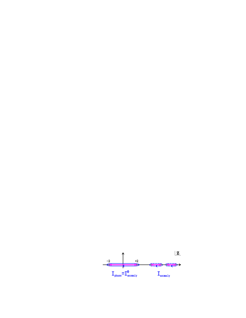
Figure 5: On $z$ plane the contributions $I_{phase}$ and $I_{anomaly}$ can be treated in absolutely equal footing. This hints the existence of an extra level in the Bethe ansatz equations whose finite size corrections would give the contribution $I_{phase}$.

Thus we would like to understand if (31) could have imprinted signs of a nested Bethe ansatz structure. Since the generalization of the Bootstrap method for the supercoset $PSU(2,2|4)$ is not known we will proceed at a rather speculative and schematic level. Let us recall that in the scaling limit the $S^{5}$ nested Bethe ansatz equations read (see e.g. equations 6.3 or 3.15 in [31])

$$/G_{\theta}+K_{\theta a}G_{a}=2\pi m\,\,\ \ \ \,\,\,\ \ \ \quad,\,\,z\in[-2,2]$$ (33)

$$/G_{a}+K_{ab}G_{b}+K_{a\theta}G_{\theta}=2\pi n_{a}\,\,,\,\,z\in\mathcal{C}_{a}$$

where the $K$’s are numeric coefficients and where the cut from $[-2,2]$ is the image of the unit circle under the Zhukovsky map. The discontinuity of $G_{\theta}$ is related to the density of the extra level particles $\theta_{\alpha}$ and is given on the $x$ plane by, roughly speaking,

$$\rho_{\theta}=-\frac{p_{2}(x)-p_{2}(1/x)}{2\pi i}\ .$$ (34)

Suppose we want to take into account $1/\sqrt{\lambda}$ corrections coming from the extra level. We denote the extra term in the first equation in (33) by $\frac{1}{\sqrt{\lambda}}V(\theta,\{u\})$. Then, if we want to eliminate $\theta$’s from this equation and plug them into the second one to obtain some effective equation for the magnons as in [34], we must solve $\delta\,/G_{\theta}=\frac{1}{\sqrt{\lambda}}V(\theta)$ and plug the solution of this Hilbert problem into the second equation. In the second equation this will then appear as an extra phase. The Hernandez-Lopez phase seems to fit into this construction. Indeed, if we go to the Zhukovsky plane in (31) through $z=x+1/x$ and $w=y+1/y$ we will have

$${\cal V}(x)=\frac{4\pi}{\sqrt{\lambda}}\int_{-2}^{2}V(w)\frac{\sqrt{4-w^{2}}}{\sqrt{z^{2}-4}}\frac{dw}{w-z}\,\,,\,\,V(w)=\frac{\partial_{w}\left[G_{4}(y)-G_{4}(1/y)\right]}{2\pi i}$$

which precisely indicates that it came from the solution of a Hilbert problem with $V(w)$ resembling the derivative of the density in (34). Indeed

$$V(w)=\partial_{w}\left[-\frac{\tilde{p}_{2}(y)-\tilde{p}_{2}(1/y)}{2\pi i}+\frac{\hat{p}_{2}(y)-\hat{p}_{2}(1/y)}{2\pi i}\right]$$

As explained in section 2 we are considering classical solutions with some large conserved charge. Then the quasi-momenta $p(x)$ scales like that charge close to the unit circle [24] and so will the density (34). Thus if we assume that the anomaly for these roots is of the usual form $\rho_{\theta}^{\prime}\coth\pi\rho_{\theta}$ we see that we can drop the cotangent with exponential precision and we are left precisely with the derivative of the density of $\theta$ particles which, as we argued above, strongly resembles $V(w)$! Moreover, the integral over the unit circle in 2b will be mapped to the cycle around the $\theta$ from $z=-2$ to $z=2$ thus leading to the very democratic figure 5.

5 Conclusions

The fluctuation energies around any classical solution can be computed from the classical algebraic curve [21] which, a priori, contains no information about the HL phase suppressed as $1/\sqrt{\lambda}$. On the other hand, if we expand the energy of some state in $1/\sqrt{\lambda}$ we will obtain the classical energy of order $\sqrt{\lambda}$ plus a finite correction which is known [22] to be the sum of these fluctuation frequencies. In other words, the sub-leading order is constrained by the leading order!

This interconnection between the leading and sub-leading terms means that, if one believes in the existence of a Bethe ansatz description of the quantum string, then the first correction to the dressing factor is completely constrained. Thus we might wonder if this procedure can be iterated to fix order by order, the full scalar factor.

In this paper we found that the first correction to the dressing factor must have the form

$${\cal V}(x)=\int_{-1}^{1}\partial_{y}\left[G_{4}(y)-G_{4}(1/y)\right]\left(\frac{\alpha(x)}{x-y}-\frac{\alpha(1/x)}{1/x-y}\right)\frac{dy}{2\pi}\,,$$

in order to accommodate for the $1/\sqrt{\lambda}$ “non-analytical” part of the $1$-loop shift for any classical configuration.

One can see that the $1/\sqrt{\lambda}$ corrections in the Beisert-Staudacher equations with the Hernandez-Lopez phase to any conserved charge $Q_{n}$ is given by one half of the graded sum of the corresponding charges of the fluctuations – as it was the case for energy.

Moreover, this representation of the phase has several interesting features. First of all, it is extremely simple – the Hernandez-Lopez coefficients follow after a trivial expansion of the resolvent in conserved charges and to find the scattering phase $\theta(x,y)$ between two magnons one merely needs to plug the definition of the resolvent into the integral without the need to perform any re-summation. By construction, the cut structure is also very clear and thus the crossing relation becomes transparent.

Finally this phase has imprinted signs pointing towards the existence of an extra level of $\theta$ roots (which are in fact rapidities of physical particles of the theory) in the Bethe ansatz equations. These extra roots live in the unit circle and in the quasi-classical limit condense into some smooth distribution whose density resembles the $G_{4}(y)-G_{4}(1/y)$ [31] appearing in $\mathcal{V}(x)$. It is very likely that the anomaly associated with the roots of this new level naturally reproduce the Hernandez-Lopez phase.

Acknowledgements

We would like to thank K. Zarembo and V. Kazakov for many useful discussions. The work of N.G. was partially supported by French Government PhD fellowship, by RSGSS-1124.2003.2 and by RFFI project grant 06-02-16786. P. V. is funded by the Fundação para a Ciência e Tecnologia fellowship SFRH/BD/17959/2004/0WA9.

Appendix A – Large $N$ limit

In the $x$ plane the contour in figure 4a is mapped to that in figure 4b. For large $N$ the contour starts at $-1-\epsilon_{-}^{ij}(N)$ and ends at $+1+\epsilon_{+}^{ij}(N)$. In this appendix we perform a careful analysis of the large $N$ limit.

A.1 Asymptotics of quasimomenta and expansion of $x_{n}$

Large $n$’s are mapped to the vicinity of $\pm 1$ where

$$\hat{p}_{2}\simeq+\frac{\alpha_{\pm}}{x\mp 1}+\sum_{n=0}\hat{a}_{n}^{\pm}(x\mp 1)^{n}\,\,,\,\,\tilde{p}_{2}\simeq+\frac{\alpha_{\pm}}{x\mp 1}+\sum_{n=0}\tilde{a}_{n}^{\pm}(x\mp 1)^{n}\,,$$

$$\hat{p}_{3}\simeq-\frac{\alpha_{\pm}}{x\mp 1}+\sum_{n=0}\hat{b}_{n}^{\pm}(x\mp 1)^{n}\,\,,\,\,\tilde{p}_{3}\simeq-\frac{\alpha_{\pm}}{x\mp 1}+\sum_{n=0}\tilde{b}_{n}^{\pm}(x\mp 1)^{n}\,.$$

The remaining quasimomenta are fixed by the $x\rightarrow 1/x$ symmetry

$$\tilde{p}_{1,2}(x) = -2\pi m-\tilde{p}_{2,1}(1/x)$$

$$\tilde{p}_{3,4}(x) = +2\pi m-\tilde{p}_{4,3}(1/x)$$ (35)

$$\hat{p}_{1,2,3,4}(x) = -\hat{p}_{2,1,4,3}(1/x)\,.$$

From this expansion we can read the large $n$ behavior of $x_{n}^{ij}$ defined by (6). Let us, however, use a more general definition

$$p_{i}(x_{n}^{ij})-p_{j}(x_{n}^{ij})=2\pi(n-m_{i}+m_{j}).$$ (36)

For $n\rightarrow\pm\infty$ all $x_{n}^{ij}$ are close to $\pm 1$ and we find

$$x_{n}^{ij}=\pm 1+\frac{\alpha^{\pm}}{\pi n}+{\cal O}\left(1/n^{2}\right)$$ (37)

where we notice that the first $1/n$ coefficient is universal and fixed uniquely by the residues of the quasi-momenta.

A.2 Large $N$ versus $\epsilon$ regularization

The main goal of this appendix is to justify the integration path used in the main text where for all $ij$ the integral in the $x$ plane starts from $-1-\epsilon$ and ends at $1+\epsilon$ as depicted on the figure 5b. However by definition (29) we have to start from the large $N$ regularization. These two regularization in principal are not equivalent, since $x_{N}^{ij}$’s are not exactly equal for all $ij$ and thus we should calculate the difference between both regularizations. For example

$$\delta V^{reg}_{k}(x)=\frac{1}{2}\lim_{N\to\infty,\epsilon\to 0}\sum_{ij}\left(\int\limits_{x^{ij}_{-N}}^{x^{ij}_{N}}-\int\limits_{-1-\epsilon}^{1+\epsilon}\right)(-1)^{F}V_{k}^{ij}(x,y)\frac{p^{\prime}_{i}(y)-p^{\prime}_{j}(y)}{2\pi}dy\,.$$ (38)

The difference of the integrals above can be rewritten as a sum of two integrals, one from $x_{-N}^{ij}$ to $-1-\epsilon$ and another from $1+\epsilon$ to $x_{N}^{ij}$, and thus we can use expansion of quasimomenta around $\pm 1$ to evaluate this $\delta V^{reg}_{k}(x)$. One can see that only first terms in (24,25) could be responsible for a non-zero difference given by

$$\delta V^{reg}_{\hat{1},\hat{2}}(x)=-\frac{\pi^{2}x}{(x^{2}-1)\sqrt{\lambda}}\left(\frac{1}{\alpha_{+}}+\frac{1}{\alpha_{-}}\right)\left(m+m_{\hat{1}}+m_{\hat{2}}-m_{\tilde{1}}-m_{\tilde{2}}\right)\left(m+m_{\tilde{3}}+m_{\tilde{4}}-m_{\hat{3}}-m_{\hat{4}}\right)$$

$$\delta V^{reg}_{\tilde{1},\tilde{2}}(x)=-\frac{\pi^{2}x}{(x^{2}-1)\sqrt{\lambda}}\left(\frac{1}{\alpha_{+}}-\frac{1}{\alpha_{-}}\right)\left(m+m_{\hat{1}}+m_{\hat{2}}-m_{\tilde{1}}-m_{\tilde{2}}\right)\left(m+m_{\tilde{3}}+m_{\tilde{4}}-m_{\hat{3}}-m_{\hat{4}}\right)\,.$$

If the potentials $V_{k}$ are to be originated from a phase in the middle note of the BS equations then they should all be equal. This means that in order to be consistent with the phase origin, these two terms should be zero. Fortunately it is possible to choose $m_{i}$ in such a way that it is so. For example

$$m_{\tilde{1}}=m\,\,,\,\,m_{\tilde{4}}=-m$$ (39)

and all the others $m_{i}$ are zero. This amounts to a different prescription for the mode numbers comparatively to [21]. For obvious reasons let us denote it by Bethe ansatz friendly prescription. Contrary to what we had in [21] we have no obvious argument, except the obvious Bethe ansatz friendliness, in favor of this new prescription. For the $sl(2)$ and $su(2)$ one cut solutions this prescription gives the same result (with exponential precision in large $\cal J$) as in [11, 13, 23].

By the same means we can see that in (26) the last term does not contribute in the Bethe ansatz friendly prescription.

References

- [1] H. Bethe, “On the theory of metals. 1. Eigenvalues and eigenfunctions for the linear atomic chain,” Z. Phys. 71, 205 (1931).
- [2] J. M. Maldacena, “The large N limit of superconformal field theories and supergravity,” Adv. Theor. Math. Phys. 2 (1998) 231 [Int. J. Theor. Phys. 38 (1999) 1113] [arXiv:hep-th/9711200]. S. S. Gubser, I. R. Klebanov and A. M. Polyakov, “Gauge theory correlators from non-critical string theory,” Phys. Lett. B 428 (1998) 105 [arXiv:hep-th/9802109]. E. Witten, “Anti-de Sitter space and holography,” Adv. Theor. Math. Phys. 2 (1998) 253 [arXiv:hep-th/9802150].
- [3] J. A. Minahan and K. Zarembo, “The Bethe-ansatz for N = 4 super Yang-Mills,” JHEP 0303 (2003) 013 [arXiv:hep-th/0212208].
- [4] N. Beisert, “The complete one-loop dilatation operator of N = 4 super Yang-Mills theory,” Nucl. Phys. B 676 (2004) 3 [arXiv:hep-th/0307015].
- [5] N. Beisert and M. Staudacher, “The N = 4 SYM integrable super spin chain,” Nucl. Phys. B 670 (2003) 439 [arXiv:hep-th/0307042].
- [6] N. Beisert, V. Dippel and M. Staudacher, “A novel long range spin chain and planar N = 4 super Yang-Mills,” JHEP 0407 (2004) 075 [arXiv:hep-th/0405001].
- [7] V. A. Kazakov, A. Marshakov, J. A. Minahan and K. Zarembo, “Classical / quantum integrability in AdS/CFT,” JHEP 0405 (2004) 024 [hep-th/0402207].
- [8] G. Arutyunov, S. Frolov and M. Staudacher, “Bethe ansatz for quantum strings,” Phys. Rev. D 66 (2002) 010001 arXiv:hep-th/0406256.
- [9] N. Beisert and M. Staudacher, “Long-range PSU(2,2—4) Bethe ansaetze for gauge theory and strings,” Nucl. Phys. B 727 (2005) 1 [arXiv:hep-th/0504190].
- [10] N. Beisert, “The su(2—2) dynamic S-matrix,” arXiv:hep-th/0511082.
- [11] S. Frolov and A. A. Tseytlin, “Multi-spin string solutions in AdS(5) x S**5,” Nucl. Phys. B 668, 77 (2003) [arXiv:hep-th/0304255]. S. Frolov and A. A. Tseytlin, “Quantizing three-spin string solution in AdS(5) x S**5,” JHEP 0307, 016 (2003) [arXiv:hep-th/0306130]. G. Arutyunov, J. Russo and A. A. Tseytlin, “Spinning strings in AdS(5) x S**5: New integrable system relations,” Phys. Rev. D 69, 086009 (2004) [arXiv:hep-th/0311004]. I. Y. Park, A. Tirziu and A. A. Tseytlin, “Spinning strings in AdS(5) x S**5: One-loop correction to energy in SL(2) sector,” JHEP 0503, 013 (2005) [arXiv:hep-th/0501203]. N. Beisert and A. A. Tseytlin, “On quantum corrections to spinning strings and Bethe equations,” Phys. Lett. B 629 (2005) 102 [arXiv:hep-th/0509084].
- [12] R. Hernandez and E. Lopez, “Quantum corrections to the string Bethe ansatz,” JHEP 0607 (2006) 004 [arXiv:hep-th/0603204].
- [13] S. Schafer-Nameki, M. Zamaklar and K. Zarembo, “Quantum corrections to spinning strings in AdS(5) x S**5 and Bethe ansatz: A comparative study,” JHEP 0509 (2005) 051 [arXiv:hep-th/0507189].
- [14] N. Beisert, A. A. Tseytlin and K. Zarembo, “Matching quantum strings to quantum spins: One-loop vs. finite-size corrections,” Nucl. Phys. B 715 (2005) 190 [arXiv:hep-th/0502173]. R. Hernandez, E. Lopez, A. Perianez and G. Sierra, “Finite size effects in ferromagnetic spin chains and quantum corrections to classical strings,” JHEP 0506 (2005) 011 [arXiv:hep-th/0502188]. N. Beisert and L. Freyhult, “Fluctuations and energy shifts in the Bethe ansatz,” Phys. Lett. B 622 (2005) 343 [arXiv:hep-th/0506243]. N. Gromov and V. Kazakov, “Double scaling and finite size corrections in sl(2) spin chain,” Nucl. Phys. B 736 (2006) 199 [arXiv:hep-th/0510194].
- [15] L. Freyhult and C. Kristjansen, “A universality test of the quantum string Bethe ansatz,” Phys. Lett. B 638 (2006) 258 [arXiv:hep-th/0604069].
- [16] R. A. Janik, “The AdS(5) x S**5 superstring worldsheet S-matrix and crossing symmetry,” Phys. Rev. D 73, 086006 (2006) [arXiv:hep-th/0603038].
- [17] A. V. Kotikov and L. N. Lipatov, “DGLAP and BFKL equations in the N = 4 supersymmetric gauge theory,” Nucl. Phys. B 661 (2003) 19 [Erratum-ibid. B 685 (2004) 405] [arXiv:hep-ph/0208220].
- [18] N. Beisert, R. Hernandez and E. Lopez, “A crossing-symmetric phase for AdS(5) x S**5 strings,” JHEP 0611 (2006) 070 [arXiv:hep-th/0609044]. N. Beisert, “On the scattering phase for AdS(5) x S**5 strings,” Mod. Phys. Lett. A 22, 415 (2007) [arXiv:hep-th/0606214].
- [19] N. Beisert, B. Eden and M. Staudacher, “Transcendentality and crossing,” J. Stat. Mech. 0701 (2007) P021 [arXiv:hep-th/0610251]. B. Eden and M. Staudacher, “Integrability and transcendentality,” J. Stat. Mech. 0611, P014 (2006) [arXiv:hep-th/0603157].
- [20] N. Beisert, V. A. Kazakov, K. Sakai and K. Zarembo, “The algebraic curve of classical superstrings on AdS(5) x S**5,” Commun. Math. Phys. 263 (2006) 659 [hep-th/0502226].
- [21] N. Gromov and P. Vieira, “The AdS(5)xS(5) superstring quantum spectrum from the algebraic curve,” arXiv:hep-th/0703191.
- [22] S. Frolov and A. A. Tseytlin, “Semiclassical quantization of rotating superstring in AdS(5) x S(5),” JHEP 0206 (2002) 007 [arXiv:hep-th/0204226].
- [23] S. Schafer-Nameki, “Exact expressions for quantum corrections to spinning strings,” Phys. Lett. B 639 (2006) 571 [arXiv:hep-th/0602214].
- [24] N. Gromov, P. Vieira, Work in progress.
- [25] D. Berenstein, J. M. Maldacena and H. Nastase, “Strings in flat space and pp waves from N=4 Super Yang Mills,” AIP Conf. Proc. 646, 3 (2003).
- [26] G. Arutyunov and S. Frolov, “Integrable Hamiltonian for classical strings on AdS(5) x S**5,” JHEP 0502 (2005) 059 [arXiv:hep-th/0411089].
- [27] N. Beisert, V. A. Kazakov, K. Sakai and K. Zarembo, “Complete spectrum of long operators in N = 4 SYM at one loop,” JHEP 0507 (2005) 030 [arXiv:hep-th/0503200].
- [28] G. Arutyunov and S. Frolov, “On AdS(5) x S**5 string S-matrix,” Phys. Lett. B 639 (2006) 378 [arXiv:hep-th/0604043].
- [29] S. Schafer-Nameki, M. Zamaklar and K. Zarembo, “How accurate is the quantum string Bethe ansatz?,” JHEP 0612 (2006) 020 [arXiv:hep-th/0610250].
- [30] N. Mann and J. Polchinski, “Bethe ansatz for a quantum supercoset sigma model,” Phys. Rev. D 72 (2005) 086002 [arXiv:hep-th/0508232].
- [31] N. Gromov, V. Kazakov, K. Sakai and P. Vieira, “Strings as multi-particle states of quantum sigma-models,” Nucl. Phys. B 764 (2007) 15 [arXiv:hep-th/0603043].
- [32] A. B. Zamolodchikov and A. B. Zamolodchikov, “Relativistic Factorized S Matrix In Two-Dimensions Having O(N) Isotopic Symmetry,” Nucl. Phys. B 133 (1978) 525 [JETP Lett. 26 (1977) 457].
- [33] A. Rej, D. Serban and M. Staudacher, “Planar N = 4 gauge theory and the Hubbard model,” JHEP 0603, 018 (2006) [arXiv:hep-th/0512077].
- [34] N. Gromov and V. Kazakov, “Asymptotic Bethe ansatz from string sigma model on S**3 x R,” arXiv:hep-th/0605026.
- [35] A. Rej, M. Staudacher and S. Zieme, “Nesting and dressing,” arXiv:hep-th/0702151.
- [36] K. Sakai and Y. Satoh, “Origin of dressing phase in N = 4 super Yang-Mills,” arXiv:hep-th/0703177.