Integrable Cosmological Models From Higher Dimensional Einstein Equations

Abstract

We consider the cosmological models for the higher dimensional spacetime which includes the curvatures of our space as well as the curvatures of the internal space. We find that the condition for the integrability of the cosmological equations is that the total space-time dimensions are $D=10$ or $D=11$ which is exactly the conditions for superstrings or M-theory. We obtain analytic solutions with generic initial conditions in the four dimensional Einstein frame and study the accelerating universe when both our space and the internal space have negative curvatures.

I Introduction

There has been much attention to the understanding cosmology from the superstring or M-theory. The recent observation of Type Ia supernovae and CMB measurement by WMAP indicates our universe is an accelerating universe. In String/M-Theory, there is the no-go theorem bio1 which is an obstacle to realize the accelerating universe. The no-go theorem indicates that the warped compactification with the static internal space does not give rise to the four-dimensional de Sitter spacetime under some assumptions. This implies that the warped compactification can not lead the accelerating universe with the static internal space.

One way to avoid the no-go theorem is to employ the time-dependent internal space bio2 . pace. If the curvature of the internal space is negative in the four-dimensional Einstein frame, it has been shown that the effective Lagrangian has positive potentials bio3 -bio7 . This positive potential gives rise to the acceleration of the four-dimensional spacetime in the four-dimensional Einstein frame. In the four-dimensional Einstein frame, the scale factor of the internal space appears as a scalar field with potentials which come from the curvature of the internal s S-brane solutions also lead to accelerating solutions bio8 -bio14 . The flux field has a role of a positive potential and contributes to the acceleration of the four-dimensional spacetime. Scalar perturbations of scale factors have been shown in bio4 that the eternally accelerating universe is realized in the eleven-dimensional spacetime by the external and internal spaces which possess a negative curvature. Recently, it has been also shown by scalar perturbations of scale factors that the eternally accelerating universe occurs in the ten-dimensional spacetime bio5 . The fixed point analysis bio29 also showed that the eternal acceleration is realized if two spaces possess a negative curvature.

In general, it is difficult to solve the Einstein equations exactly because of the non-linearity of the Einstein equations. Therefore, most of the analytic solutions are special solutions with particular initial conditions. However, it is desirable to find integrable models for the analysis of the initial conditions for our universe. Up to now, few integrable models have been found. In $p$-brane and cosmological solutions which were inspired with String/M-theory, it is known that there exist a few classes of models whose solutions can be reduced to the Liouville or Toda type bio15 -bio21 . The Toda equation is integrable and provides exact solutions for us. In bio15 -bio21 , the metric has two spatial parts whose curvature is flat for all spaces or for one of two spaces. However, if both spaces have curvatures, it is very difficult to solve even vacuum Einstein equations exactly. When our universe starts from the quantum era, it is natural to expect that we have spatial curvatures whose values are comparable with the curvature to the direction of time. The curvatures with respect to the spatial directions can be regarded as potential energies whereas the time dependence can be regarded as the kinetic energy of the effective actions. If the universe started from quantum fluctuations, it is natural to expect that the order of the potential energies are the same as the order of the kinetic energy. Therefore, it is highly desirable to find integrable models with spatial curvatures both for our space and the internal space.

The accelerating universe occurs when two spatial parts have the negative curvature as shown in bio4 -bio5 . This analysis performed by the perturbation of scale factors. In bio29 the fixed point analysis was performed and also showed that the eternally accelerating universe occurs with two spatial parts whose curvature is negative. In this paper, we will try to solve $D$-dimensional vacuum Einstein equations with two homogeneous spaces exactly.

In order to find integrable cosmological models, we will adopt a method for solving Einstein equations analyzed in bio22 . In the method used in bio22 , the Einstein equations can be reduced to an analytically mechanical problem with one gauge degree of freedom. The gauge degree of freedom originates from the choice of the time variable. By using time variables which include scalar fields, the condition of the integrability has been classified. We will review this method in the next section and find that we are able to obtain general solutions for those vacuum Einstein equations. Actually, it will turn out that the classification of bio22 was not complete and we will show that a new type of integrable models is useful for our analysis.

We will start with the generic space ansatz with total dimensions $D$ and our spatial dimensions $d$. Strangely enough, we will find that the condition for the integrability is that the total dimension is ten or eleven, which is exactly correspond to the consistency conditions of superstrings or M-theory. If the integrable condition is satisfied there is an additional conserved quantity aside from the Hamiltonian constraint. Therefore the system has two conserved quantities for two dynamical variables and then the system reduces to the integrable case.

In bio26 -bio28 , the relation between the integrable condition and the conserved quantity was investigated from the Hamiltonian viewpoint. The same integrability condition was obtained and it was shown that there exist the conserved quantity under the integrability condition.

The integrable system does not necessarily have the simple analytic solutions bio26 -bio28 . In this paper, it will be shown that we are able to derive the analytic solutions by the particular choices of the time variable in $D=10$ and $D=11$. It is very important to note that the time variable used in this paper easily realizes the analytic solutions. The other choices of the time variable make it difficult to solve the equations of motion.

We investigated the cosmological behavior in $D=10$ because this case includes the four-dimensional spacetime and the six-dimensional internal space. It was found that the accelerating universe occurs if two spaces have a negative curvature.

This paper is organized as follows. In the next section, we will construct the effective action which has two potential terms arising from curvatures of the two spaces. We will also show that the system is integrable when the total dimensions of the space-time is ten or eleven. In section three, we will solve Einstein equations completely and general solutions will be given. In section four, we will consider the cosmological property of the case of ($D=10,\,d=3$) in detail and the analytic solutions representing the accelerating universe when two spatial parts have negative curvature. The asymptotic behavior of the metric is also discussed. Finally, we conclude with a discussion of our results and some implications.

II Effective Action and conditions for integrability

Let us consider the $D$-dimensional spacetime constructed with two spatial parts which have curvatures. For simplicity, we will consider the vacuum Einstein Equations. We consider that the $D$-dimensional space consists of two homogeneous spaces whose sizes depend on time. Namely, the metric ansatz for the $D$-dimensional spacetime is given by,

$$ds_{D}^{2} =G_{MN}(X)\,dX^{M}dX^{N}$$

$$=-e^{2\,\widetilde{n}(t)}dt^{2}+e^{2\,\widetilde{A}(t)}g_{ij}(x)\,dx^{i}dx^{j}$$

$$\qquad\qquad\qquad\qquad+e^{2\,\alpha(t)}g_{AB}(y)\,dy^{A}dy^{B},$$ (1)

where

$$\begin{cases}i,\,j=1,\,2,\,\cdots,\,d\\ A,\,B=d+1,\,d+2,\,\cdots,\,D-1\\ M,\,N=0,\,1,\,\cdots,\,D-1.\\ \end{cases}$$

$e^{2\,\widetilde{A}(t)}$ and $e^{2\,\alpha(t)}$ are scale factors of the $d$- and $(D-d-1)$-dimensional spaces whose metrics are $g_{ij}(x)\,dx^{i}dx^{j}$ and $g_{AB}(y)\,dy^{A}dy^{B}$. respectively. These scale factors depend on time variable $t$.

We assume that both two spatial manifolds are homogeneous spaces (Einstein spaces);

$${}^{(d)}\widetilde{R}_{ij}(g(x)) =(d-1)\,k_{(d)}\,g_{ij}(x),$$ (2)

$${}^{(D-d-1)}\widetilde{R}_{AB}(g(y)) =(D-d-2)\,k^{\prime}_{(D-d-1)}\,g_{AB}(y),$$ (3)

where $k_{(d)}$ and $k^{\prime}_{(D-d-1)}$ represent the curvature of Einstein spaces. For our physical $d$-dimensional space, we assume homogeneous and isotropic space. However we do not need the explicit representation of $g_{ij}(x)$ and $g_{AB}(y)$ to derive the effective action.

The ($d+1$)-dimensional Einstein frame is realized by the following conformal transformations;

$$\begin{split}&\widetilde{A}(t)\longrightarrow A(t)-\frac{1}{d-1}\,(D-d-1)\,\alpha(t),\\ &\widetilde{n}(t)\longrightarrow n(t)-\frac{1}{d-1}\,(D-d-1)\,\alpha(t).\end{split}$$ (4)

In fact, the $D$-dimensional Einstein$-$Hilbert Lagrangian can be written as

$$\begin{split}\sqrt{-G}\,R&=\sqrt{-g_{d+1}(x)\,g_{D-d-1}(y)}\,e^{d\,\widetilde{A}+\widetilde{n}+(D-d-1)\,\alpha}\,R\\ \longrightarrow&\sqrt{-g_{d+1}(x)\,g_{D-d-1}(y)}\,e^{d\,A+n}\,(\,{}^{(d+1)}R+\cdots\,).\end{split}$$

Under the conformal transformation (4), we obtain an effective action in the ($d+1$)-dimensional Einstein frame bio3 ;

$$\begin{split}&\frac{1}{d(d-1)\,V_{D-1}}\int d^{D}X\,\sqrt{-G}\,R\\ \longrightarrow&\int dt\,\Biggl{[}e^{dA-n}\,\Bigl{\{}-\dot{A}^{2}+X^{2}\,\dot{\alpha}^{2}\Bigr{\}}\\ &-e^{dA+n}\Bigl{\{}\,-k_{(d)}\,e^{-2A}-\widetilde{k}_{(D-d-1)}\,e^{-\frac{2(D-2)}{d-1}\,\alpha}\,\Bigr{\}}\Biggr{]},\end{split}$$ (5)

where $V_{D-1}\equiv\int d^{D-1}X\,\sqrt{-\det g_{ij}(x)}\,\sqrt{\det g_{AB}(y)}$ and

$$\begin{split}X^{2}&=\frac{(D-d-1)(D-2)}{d(d-1)^{2}},\\ \widetilde{k}_{(D-d-1)}&=\frac{(D-d-1)(D-d-2)}{d(d-1)}\,k^{\prime}_{(D-d-1)}.\end{split}$$ (6)

The effective action (5) shows that the scale factor of the internal space appears as a scalar field with the potential terms. The two effective potentials are generated by the curvature of Einstein spaces which can be easily seen from the fact that the potential terms are directly proportional to the curvatures.

We would like to solve equations of motion derived from the ($d+1$)-dimensional effective action (5). In general, Einstein equations are highly non-linear equations and difficult to be solved exactly. The effective action (5) indeed results in non-linear equations. A way to analyze the system is to utilize a gauge degree of freedom bio24 . Let us recall that we can choose a time variable via the lapse function $e^{n(t)}$ which is a non-dynamical quantity bio24 . This gauge degree of freedom represents the invariance under the coordinate transformation of time. Because of this gauge degree of freedom, we can freely choose the gauge to solve the system. We will take the lapse function as

$$e^{n(t)}=e^{p\,\alpha(t)+q\,A(t)},$$ (7)

where $p$ and $q$ are any real numbers. We would like to look for the more convenient transformation of two dynamical variables.

We use the following transformation between ($A,\,\alpha$) and ($U_{+},\,U_{-}$),

$$e^{2A} =U_{+}^{\frac{M_{1}+1}{d-1}}\,U_{-}^{\frac{M_{2}+1}{d-1}},$$

$$e^{2\alpha} =U_{+}^{\frac{(M_{1}+1)}{(d-1)\,X}}\,U_{-}^{-\frac{(M_{2}+1)}{(d-1)\,X}},$$ (8)

$$e^{2n} =U_{+}^{-2+\frac{d\,(M_{1}+1)}{d-1}}\,U_{-}^{-2+\frac{d\,(M_{2}+1)}{d-1}},$$

where we have defined

$$\begin{split}M_{1}=\frac{(d-2+q)\,X+p}{(d-q)\,X-p},\\ M_{2}=\frac{(d-2+q)\,X-p}{(d-q)\,X+p}.\end{split}$$ (9)

By using these variables, we can re-write the effective action (5) as bio22

$$\mathcal{L}_{\text{eff}}=-\frac{(M_{1}+1)(M_{2}+1)}{(d-1)^{2}}\,\dot{U}_{+}\dot{U}_{-}+k_{(d)}\,U_{+}^{M_{1}}U_{-}^{M_{2}}$$

$$+\widetilde{k}_{(D-d-1)}\,U_{+}^{-1+\frac{M_{1}+1}{d-1}\Bigl{[}d-\frac{D-2}{(d-1)X}\Bigr{]}}U_{-}^{-1+\frac{M_{2}+1}{d-1}\Bigl{[}d+\frac{D-2}{(d-1)X}\Bigr{]}}.$$ (10)

The effective action $\int dt\mathcal{L}_{\text{eff}}(M_{1},\,M_{2})$ can be transformed to the action of some other parameters $N_{1},N_{2}$, $\int d\xi\mathcal{L}_{\text{eff}}(N_{1},\,N_{2})$ by the change of time coordinates, $dt=N(\xi)\,d\xi$. This is realized by following transformations;

$$\begin{split}&U_{+}=V_{+}^{\frac{N_{1}+1}{M_{1}+1}},\quad U_{-}=V_{-}^{\frac{N_{2}+1}{M_{2}+1}},\\ &N=V_{+}^{-1+\frac{N_{1}+1}{M_{1}+1}}V_{-}^{-1+\frac{N_{2}+1}{M_{2}+1}}.\end{split}$$ (11)

These transformations preserve the form of the effective action (10). It is possible to connect a solution in some parameters ($M_{1},\,M_{2}$) to many other solutions by above transformations (11). Because of this gauge degree of freedom, we can solve the Einstein equations with a particular choice of the parameters.

In bio22 , $M_{1}=M_{2}=0$ was considered. In our cases, this condition leads the following potential

$$W =-k_{(d)}$$

$$-\widetilde{k}_{(D-d-1)}U_{+}^{-1+\frac{1}{d-1}\Bigl{[}d-\frac{D-2}{(d-1)X}\Bigr{]}}U_{-}^{-1+\frac{1}{d-1}\Bigl{[}d+\frac{D-2}{(d-1)X}\Bigr{]}}.$$

If the form of the potential becomes $W=-k_{(d)}-\widetilde{k}_{(D-d-1)}\,U_{+}$ or $W=-k_{(d)}-\widetilde{k}_{(D-d-1)}\,U_{-}$, Einstein equations are soluble as shown in bio22 . A model with this type of the potential also studied in bio25 . But the above potential cannot take such that potential because the total dimension has to be $D=1$ in order to satisfy $-1+\frac{1}{d-1}\,\Bigl{[}\,d\pm\frac{D-2}{(d-1)X}\,\Bigr{]}=0$. Therefore our model is not correspond to the model considered in bio22 .

A convenient choice of the parameters is $M_{1}=M_{2}=1$ which implies

$$\mathcal{L}_{\text{eff}}=-\frac{4}{(d-1)^{2}}\,\dot{U}_{+}\dot{U}_{-}+k_{(d)}\,U_{+}\,U_{-}$$

$$+\widetilde{k}_{(D-d-1)}\,U_{+}^{-1+\frac{2}{d-1}\,\Bigl{[}\,d-\frac{D-2}{(d-1)X}\,\Bigr{]}}U_{-}^{-1+\frac{2}{d-1}\,\Bigl{[}\,d+\frac{D-2}{(d-1)X}\,\Bigr{]}}.$$ (12)

The above effective Lagrangian shows the second term is an interaction similar to a harmonic oscillator and third term represents a non-linear interaction which is an obstacle to solve equations of motion. If the power of $U_{+}$ or $U_{-}$ is simplified, it is possible to solve the equations analytically. To perform this procedure, we will impose a condition in which the non-linear term in the effective action does not depend on $U_{+}$;

$$-1+\frac{2}{d-1}\,\Bigl{[}\,d-\frac{D-2}{(d-1)X}\Bigr{]}=0,$$ (13)

where $X$ was defined in (6). We will see below that the system is integrable if this condition is satisfied. Before considering the integrability, let us solve the condition (13). The condition (13) can be rewritten as

$$(d-1)(D-d-5)=4.$$ (14)

From this, we can immediately derive the condition of the integrability $D$ and $d$ as follows

$$\begin{cases}D=10,\qquad d=3\\ D=11,\qquad d=2,\,5,\end{cases}$$ (15)

where (6) was used. Note that $D=10$ is the critical dimension of the superstring theories and $D=11$ is the dimension of the M-theory! Moreover, $d=3$ means our spacetime is four dimensions. Therefore, we have integrable cosmological models for a realistic setup.

We are going to show that the system is integrable if the condition (13) is satisfied. By using the condition, we can rewrite the effective Lagrangian and the Hamiltonian constraint as

$$\mathcal{L}_{\text{eff}} =-\frac{4}{(d-1)^{2}}\,\dot{U}_{+}\dot{U}_{-}+k_{(d)}\,U_{+}U_{-}$$

$$\qquad\qquad\qquad\qquad+\widetilde{k}_{(D-d-1)}\,U_{-}^{2(d+1)/(d-1)},$$ (16)

$$H =0=-\frac{4}{(d-1)^{2}}\,\dot{U}_{+}\dot{U}_{-}-k_{(d)}\,U_{+}U_{-}$$

$$\qquad\qquad\qquad\qquad-\widetilde{k}_{(D-d-1)}\,U_{-}^{2(d+1)/(d-1)},$$ (17)

where the second equation represents the total energy conservation which can be derived by the variation of $n(t)$ in the action (5).

We get equations of motion by the variation with respect to $U_{+}$ and $U_{-}$ as follows

$$-\frac{4}{(d-1)^{2}}\,\ddot{U}_{+}-k_{(d)}\,U_{+}$$

$$\qquad\qquad-\widetilde{k}_{(D-d-1)}\,\frac{2(d+1)}{d-1}\,U_{-}^{(d+3)/(d-1)}=0,$$ (18)

$$-\frac{4}{(d-1)^{2}}\,\ddot{U}_{-}-k_{(d)}\,U_{-}=0.$$ (19)

Because of the equation (19), we can easily find the following conserved quantities;

$$\epsilon=\frac{2}{(d-1)^{2}}\dot{U}_{-}^{2}+\frac{k_{(d)}}{2}{U}_{-}^{2}.$$ (20)

Since the system has two conserved constants (17) and (20) for two dynamical variables, the total system is classically integrable.

In bio26 -bio28 , the integrability was discussed from the Hamiltonian viewpoint. It is essential idea that they looked not only for functions Poisson-commuting with the Hamiltonian $H$, but also for a function $F$ satisfying an equation of the form

$$\{F,\,H\}_{\text{P.B.}}=\phi H$$

for some unknown function $\phi$. The Hamiltonian constraint $H=0$ indicates $\{F,\,H\}_{\text{P.B.}}=\phi H=0$, therefore the function $F$ becomes a conserved quantity on this Hamiltonian constraint. Using this method, same consequence (15) was obtained in bio26 -bio28 . In our model, $\epsilon$ satisfies $\{\epsilon,\,H\}_{\text{P.B.}}=0$ where we used canonical momenta $P_{+}=-(4/(d-1)^{2})\dot{U}_{-}$, $P_{-}=-(4/(d-1)^{2})\dot{U}_{+}$, the Hamiltonian (17) and the Poisson bracket

$$\{q_{1},\,q_{2}\}_{\text{P.B.}}\equiv\sum_{i=+,-}\Biggl{[}\frac{\partial q_{1}}{\partial U_{i}}\frac{\partial q_{2}}{\partial P_{i}}-\frac{\partial q_{1}}{\partial P_{i}}\frac{\partial q_{2}}{\partial U_{i}}\Biggr{]}.$$

$\epsilon$ commutes with the Hamiltonian and then is a conserved quantity. This means that the system becomes integrable, because the system has two conserved quantities for two dynamical variables. If the condition (13) is not satisfied, $\epsilon$ dose not commute with the Hamiltonian derived from (12) and $\{\epsilon,\,H\}_{\text{P.B.}}\neq\phi H$. In the next section, we are going to show that it is quite easy to derive the analytic solutions by the choice of the time variable, ($M_{1}=M_{2}=1$).

We can impose the other type of requirement that the non-linear term in the effective action (12) does not depend on $U_{+}$. It turns out that interchanging $U_{+}$ and $U_{-}$ can be achieved by the replacement $d\rightarrow D-d-1$ which means that the interchange of the internal and the external space. This symmetry should be present because we are just considering the evolution of two homogeneous spaces. At the level of the effective action this equivalence results from the re-parametrization of the time coordinate. For instance, we will take $-1+\frac{M_{1}+1}{d-1}\,\Bigl{[}\,d-\frac{D-2}{(d-1)X}\,\Bigr{]}=-1+\frac{M_{2}+1}{d-1}\,\Bigl{[}\,d+\frac{D-2}{(d-1)X}\,\Bigr{]}=1$ in (10) and impose $-1+\frac{2(d-1)}{d-(D-2)/(d-1)X}=0$ which gives

$$\begin{cases}D=10,\qquad d=6\\ D=11,\qquad d=5,\,8\end{cases}$$ (21)

where we have used (6). The effective Lagrangian is identical to (16) just by interchanging the two spaces.

III General Solutions

In the previous section, we have seen that the Einstein equations for two homogeneous spaces are integrable if the total dimensions are ten or eleven. In this section, we will discuss the case $D=10,\,d=3$ which is most relevant for four-dimensional physics. General solutions of ($D=11,\,d=2$) and ($D=11,\,d=5$) are shown in Appendix A.

In this case, the equations of motion (18)-(19) and the Hamiltonian constraint (17) are written by

$$\ddot{U}_{+}+k_{(3)}\,U_{+}+4\,\widetilde{k}_{(6)}\,U_{-}^{3}=0,$$ (22)

$$\ddot{U}_{-}+k_{(3)}\,U_{-}=0,$$ (23)

$$\dot{U}_{+}\dot{U}_{-}+k_{(3)}\,U_{+}U_{-}+\widetilde{k}_{(6)}\,U_{-}^{4}=0,$$ (24)

where $\widetilde{k}_{(6)}=5\,k^{\prime}_{(6)}$. Let us first consider the equation of motion (23). The solution of (23) can be easily obtained as

$$U_{-}=\begin{cases}A_{1}\,\cos[\,\sqrt{k_{(3)}}\,t+A_{2}\,],\qquad~{}~{}\,(k_{(3)}>0)\\ A_{1}\,t+A_{2},\qquad\qquad\qquad~{}~{}~{}~{}\,~{}\,(k_{(3)}=0)\\ A_{1}\,\cosh[\,\sqrt{-k_{(3)}}\,t+A_{2}\,],\quad~{}\,(k_{(3)}<0)\end{cases}$$ (25)

where $A_{1}$ and $A_{2}$ are constants of integrations. These equations show that the behavior of $U_{-}$ is controlled by the curvature of the three-dimensional Einstein space. Substituting this $U_{-}$ into the equation of motion (22), we obtain following equations of motion,

$$\begin{split}&k_{(3)}>0\,;\quad\ddot{U}_{+}+k_{(3)}\,U_{+}\\ &\qquad\qquad\quad+4\,\widetilde{k}_{(6)}\,\Bigl{(}\,A_{1}\,\cos[\,\sqrt{k_{(3)}}\,t+A_{2}\,]\,\Bigr{)}^{3}=0,\\ &k_{(3)}=0\,;\quad\ddot{U}_{+}+4\,\widetilde{k}_{(6)}\,\Bigl{(}\,A_{1}\,t+A_{2}\,\,\Bigr{)}^{3}=0,\\ &k_{(3)}<0\,;\quad\ddot{U}_{+}+k_{(3)}\,U_{+}\\ &\qquad\qquad+4\,\widetilde{k}_{(6)}\,\Bigl{(}\,A_{1}\,\cosh[\,\sqrt{-k_{(3)}}\,t+A_{2}\,]\,\Bigr{)}^{3}=0.\end{split}$$ (26)

These equations of motion concretely show that the $U_{+}$ have received the forced power from the $U_{-}$. The internal space gives the effect of the forced oscillation to the motion of $U_{+}$.

In the cases of $k_{(3)}<0$ or $k_{(3)}>0$, it is useful to adopt the following transformations;

$$\begin{split}&k_{(3)}>0\,;\quad U_{+}=f(t)\\ &\qquad\qquad\qquad\qquad-\frac{3\,\widetilde{k}_{(6)}A_{1}^{3}}{2\,\sqrt{k_{(3)}}}\,t\,\sin[\,\sqrt{k_{(3)}}\,t+A_{2}\,]\\ &\qquad\qquad\qquad\qquad+\frac{\widetilde{k}_{(6)}A^{3}_{1}}{8\,k_{(3)}}\,\cos[\,3(\,\sqrt{k_{(3)}}\,\,t+A_{2}\,)\,]\\ &k_{(3)}<0\,;\quad U_{+}=f(t)\\ &\qquad\qquad\qquad\qquad-\frac{3\,\widetilde{k}_{(6)}A_{1}^{3}}{2\,\sqrt{-k_{(3)}}}\,t\,\sinh[\,\sqrt{-k_{(3)}}\,t+A_{2}\,]\\ &\qquad\qquad\qquad\qquad+\frac{\widetilde{k}_{(6)}A^{3}_{1}}{8\,k_{(3)}}\,\cosh[\,3(\,\sqrt{-k_{(3)}}\,\,t+A_{2}\,)\,]\end{split}$$ (27)

Using these relations, we can simplify the equation of motion (26) as

$$\begin{split}&\ddot{f}(t)+k_{(3)}\,f(t)=0,\qquad~{}~{}~{}~{}\,\,(\,k_{(3)}>0\,)\\ &\ddot{f}(t)+(\,-k_{(3)}\,)\,f(t)=0.\qquad(\,k_{(3)}<0\,)\end{split}$$

Then, answers for this equation are simply

$$\begin{split}&f(t)=B_{1}\,\cos[\,\sqrt{k_{(3)}}\,\,t+B_{2}\,],(k_{(3)}>0)\\ &f(t)=B_{1}\,\sinh[\,\sqrt{-k_{(3)}}\,\,t+B_{2}\,],(k_{(3)}<0)\end{split}$$

where $B_{1}$ and $B_{2}$ are the constants of integrations. Combining all these things, we finally obtain the solutions given by

$$\begin{split}&k_{(3)}>0\,;\quad U_{+}=B_{1}\,\cos[\,\sqrt{k_{(3)}}\,\,t+B_{2}\,]\\ &\qquad\qquad\qquad\qquad-\frac{3\,\widetilde{k}_{(6)}A_{1}^{3}}{2\,\sqrt{k_{(3)}}}\,t\,\sin[\,\sqrt{k_{(3)}}\,t+A_{2}\,]\\ &\qquad\qquad\qquad\qquad+\frac{\widetilde{k}_{(6)}A^{3}_{1}}{8\,k_{(3)}}\,\cos[\,3(\,\sqrt{k_{(3)}}\,\,t+A_{2}\,)\,],\\[6.0pt] &k_{(3)}=0\,;\quad U_{+}=B_{1}\,t+B_{2}-\frac{\widetilde{k}_{(6)}}{5A^{2}_{1}}\,(A_{1}\,t+A_{2})^{5},\\[7.0pt] &k_{(3)}<0\,;\quad U_{+}=B_{1}\,\sinh[\,\sqrt{-k_{(3)}}\,\,t+B_{2}\,]\\ &\qquad\qquad\qquad\quad-\frac{3\,\widetilde{k}_{(6)}A_{1}^{3}}{2\,\sqrt{-k_{(3)}}}\,t\,\sinh[\,\sqrt{-k_{(3)}}\,t+A_{2}\,]\\ &\qquad\qquad\qquad\quad+\frac{\widetilde{k}_{(6)}A^{3}_{1}}{8\,k_{(3)}}\,\cosh[\,3(\,\sqrt{-k_{(3)}}\,\,t+A_{2}\,)\,].\end{split}$$ (28)

The term proportional to $\widetilde{k}_{(6)}$ indicates the resonance, as the frequency of the harmonic and forced oscillation are identical.

The Hamiltonian constraint (24) gives a constraint on four constants of integrations,

$$\begin{split}&k_{(3)}>0\,;\quad\frac{9\widetilde{k}_{(6)}A^{3}_{1}}{8}+k_{(3)}\,B_{1}\,\cos[A_{2}-B_{2}]=0,\\ &k_{(3)}=0\,;\quad B_{1}=0,\\ &k_{(3)}<0\,;\quad\frac{9\widetilde{k}_{(6)}A^{3}_{1}}{8}+(-k_{(3)})\,B_{1}\,\sinh[A_{2}-B_{2}]=0.\end{split}$$ (29)

We shall consider the metric which is given by

$$e^{2n}=e^{2A}=U_{+}U_{-},\qquad e^{2\alpha}=\sqrt{\frac{U_{+}}{U_{-}}},$$ (30)

where we have used (6), (8) and $M_{1}=M_{2}=1$. These equations shows that the four-dimensional part is the conformal metric, $e^{2n}=e^{2A}$. Therefore, in the four-dimensional Einstein frame, ten-dimensional metric is

$$ds_{10}^{2} =e^{-6\alpha}[\,e^{2A}(-dt^{2}+g_{ij}(x)\,dx^{i}dx^{j})\,]$$

$$\qquad\qquad\qquad\qquad+e^{2\alpha}\,g_{AB}(y)\,dy^{A}dy^{B}$$

$$=\Bigg{(}\frac{U_{+}}{U_{-}}\Biggr{)}^{-3/2}\,\Bigl{[}U_{+}U_{-}\,(-dt^{2}+g_{ij}(x)\,dx^{i}dx^{j})\Bigr{]}$$

$$\qquad\qquad\qquad+\Biggl{(}\frac{U_{+}}{U_{-}}\Biggr{)}^{1/2}\,g_{AB}(y)\,dy^{A}dy^{B}.$$ (31)

For $\widetilde{k}_{(6)}\neq 0$, metric components are

$$(\,k_{(3)}>0\,)$$

$$e^{2A}=\frac{9\widetilde{k}_{(6)}A^{4}_{1}}{8\,k_{(3)}}\,\Biggl{[}-\frac{\cos[\,\sqrt{k_{(3)}}\,\,t+B_{2}\,]}{\cos[A_{2}-B_{2}]}$$

$$-\frac{4\sqrt{k_{(3)}}}{3}\,\,t\,\sin[\,\sqrt{Y_{(3)}}\,t+A_{2}\,]$$

$$+\frac{1}{9}\,\cos[\,3(\,\sqrt{k_{(3)}}\,\,t+A_{2}\,)\,]\Biggr{]}\,\cos[\,\sqrt{k_{(3)}}\,t+A_{2}\,],$$

$$e^{2\alpha}=\sqrt{\frac{9\widetilde{k}_{(6)}A^{2}_{1}}{8\,k_{(3)}}}\,\Biggl{\{}\Biggl{[}-\frac{\cos[\,\sqrt{k_{(3)}}\,\,t+B_{2}\,]}{\cos[A_{2}-B_{2}]}$$

$$-\frac{4\sqrt{k_{(3)}}}{3}\,\,t\,\sin[\,\sqrt{k_{(3)}}\,t+A_{2}\,]$$

$$+\frac{1}{9}\,\cos[\,3(\,\sqrt{k_{(3)}}\,\,t+A_{2}\,)\,]\Biggr{]}\,\frac{1}{\cos[\,\sqrt{k_{(3)}}\,t+A_{2}\,]}\Biggr{\}}^{\frac{1}{2}},$$

$$(\,k_{(3)}=0\,)$$

$$e^{2A}=\Biggl{[}-\frac{\widetilde{k}_{(6)}}{5A^{2}_{1}}\,(A_{1}\,t+A_{2})^{5}+B_{2}\Biggr{]}\,(A_{1}\,t+A_{2}),$$

$$e^{2\alpha}=\Biggl{\{}\Biggl{[}-\frac{\widetilde{k}_{(6)}}{5A^{2}_{1}}\,(A_{1}\,t+A_{2})^{5}+B_{2}\Biggr{]}\frac{1}{A_{1}\,t+A_{2}}\Biggr{\}}^{\frac{1}{2}},$$

$$(\,k_{(3)}<0\,)$$

$$e^{2A}=\frac{-9\widetilde{k}_{(6)}A^{4}_{1}}{8\,(-k_{(3)})}\,\Biggl{[}\frac{\sinh[\,\sqrt{-k_{(3)}}\,\,t+B_{2}\,]}{\sinh[A_{2}-B_{2}]}$$

$$+\frac{4\sqrt{-k_{(3)}}}{3}\,\,t\,\sinh[\,\sqrt{-k_{(3)}}\,t+A_{2}\,]$$

$$+\frac{1}{9}\cosh[\,3(\,\sqrt{-k_{(3)}}\,\,t+A_{2}\,)\,]\Biggr{]}\cosh[\,\sqrt{-k_{(3)}}\,t+A_{2}\,],$$

$$e^{2\alpha}=\sqrt{\frac{-9\widetilde{k}_{(6)}A^{2}_{1}}{8\,(-k_{(3)})}}\,\Biggl{\{}\Biggl{[}\frac{\sinh[\,\sqrt{-k_{(3)}}\,\,t+B_{2}\,]}{\sinh[A_{2}-B_{2}]}\,$$

$$+\frac{4\sqrt{-k_{(3)}}}{3}\,\,t\,\sinh[\,\sqrt{-k_{(3)}}\,t+A_{2}\,]$$

$$+\frac{1}{9}\cosh[3(\,\sqrt{-k_{(3)}}\,\,t+A_{2}\,)\,]\Biggr{]}\,\frac{1}{\cosh[\sqrt{-k_{(3)}}\,t+A_{2}]}\Biggr{\}}^{\frac{1}{2}}.$$ (32)

IV Cosmological Characteristic for (D=10, d=3)

The solutions that we have obtained in the previous section include a metric which has realistic dimensions $D=10,\,d=3$. The total dimension of this spacetime is ten dimension equal to the critical dimension of superstrings and the physical space-time has four dimensions. Therefore, it is very interesting how the universe evolve with time. In this section, we shall consider the behavior of the ten-dimensional spacetime. We will analytically show that the four-dimensional part of the ten-dimensional spacetime accelerates eternally, which has been analyzed in bio5 by the qualitative method and in bio29 by the fixed point analysis on the phase space.

We shall consider metric (32). In $k_{(3)}>0$, $e^{2\,A}$ and $e^{2\,\alpha}$ take oscillatory behavior. $e^{2\,A}$ starts from zero and end up with zero because $U_{-}=A_{1}\,\cos[\sqrt{k_{(3)}}\,t+A_{1}]$ oscillates between two zeros. On the other hand, $e^{2\,\alpha}$ diverges when $U_{-}$ and $e^{2\,A}$ become zero, and then, the case of $k_{(3)}>0$ may not have a stable internal space.

Similarly, in $k_{(3)}=0$, the scale factor of the internal space diverges at $U_{-}=A_{1}\,t+A_{2}=0$ and $e^{2\,A}$ takes zero when $U_{-}=0$. For $k_{(3)}=0$ and $\widetilde{k}_{6}<0$, the asymptotic behavior becomes $e^{2\,A}\rightarrow t^{6}$ and $e^{2\,\alpha}\rightarrow t^{2}$ at $t\rightarrow\infty$ and the ten-dimensional metric (31) has the behavior as follows

$$ds_{10}^{2}\rightarrow(\,-dt^{2}+ds_{3}^{2}\,)+t^{2}\,ds_{6}^{2}.$$ (33)

This means that the four-dimensional part of the metric does not depend on $t$ in the ten-dimensional frame. If we take $ds^{2}_{3}$ to the three-dimensional Euclid space, the four-dimensional part becomes the Minkowski spacetime at $t\rightarrow\infty$. The internal space becomes large in this region.

If $k_{(3)}<0$, an interesting phenomenon occurs. The three-dimensional space expands with acceleration eternally. This acceleration is extracted from the negative curvature of the internal space, $\widetilde{k}_{(6)}<0$. The curvature of the internal space acts like a positive cosmological constant in four dimensions. We assume the internal space is the Einstein space with the negative curvature. This case, $k_{(3)}<0$ and $\widetilde{k}_{(6)}<0$, is equivalent to the situation suggested in bio5 in which it was shown by scalar perturbations of scale factors that the acceleration of the three-dimensional space occurs in the four-dimensional Einstein frame. In bio29 the fixed point analysis also indicated that the eternal acceleration occurs for $k_{(3)}<0$ and $\widetilde{k}_{(6)}<0$. We can confirm these facts by using the analytic solutions.

Defining a proper time $d\tau\equiv\sqrt{U_{+}\,U_{-}}\,dt$, the velocity and acceleration of $e^{A}$ are given by $de^{A}/d\tau$ and $d^{2}e^{A}/d\tau^{2}$. These velocity and acceleration are shown in fig.[1]-[2] where we neglect overall factor in (32).

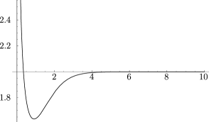
Figure 1: The velocity of $e^{A}$. $k_{(3)}=-1$, $A_{2}=0.5$, $B_{2}=0$.

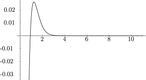
Figure 2: The acceleration of $e^{A}$. $k_{(3)}=-1$, $A_{2}=0.5$, $B_{2}=0$.

From these figures, we can extract following facts. The three-dimensional space evolves with the very large positive velocity and negative acceleration, then the three-dimensional space decelerates quickly at a first stage. The acceleration of the three-dimensional space turns to positive at some time, and then the acceleration decreases gradually. The three-dimensional space finally expands with a positive velocity and the zero acceleration at the infinite future. In particular, the three-dimensional space accelerates forever. This fact coincides with bio5 and bio29 .

We shall consider the asymptotic behavior of $e^{2\,A}$ and $e^{2\,\alpha}$ in (32). $U_{-}=A_{1}\,\cosh[\sqrt{-k_{(3)}}\,t+A_{2}]$ is not singular for appropriate constants of integrations. $A_{1}$ and $A_{2}$, which implies $e^{2\,\alpha}$ may not diverge when $e^{2\,A}\rightarrow 0$. For $t\rightarrow\infty$, $e^{2\,A}\rightarrow e^{4\,\sqrt{-k_{(3)}}\,t}$, $e^{2\,\alpha}\rightarrow e^{\,\sqrt{-k_{(3)}}\,t}$ and

$$ds^{2}_{10}\rightarrow e^{\,\sqrt{-k_{(3)}}\,t}(\,-dt^{2}+ds^{2}_{3}+ds^{2}_{6}\,).$$ (34)

It is found that this ten-dimensional metric is conformally equivalent to $-dt^{2}+ds^{2}_{3}+ds^{2}_{6}$ at large $t$. In four-dimensional Einstein frame, this metric (34) behaves as

$$\begin{split}ds^{2}_{10}\rightarrow&e^{\,-3\sqrt{-k_{(3)}}\,t}[e^{\,4\sqrt{-k_{(3)}}\,t}(-dt^{2}+ds^{2}_{3})]\\ &\qquad\qquad\qquad\qquad\qquad\quad+e^{\,\sqrt{-k_{(3)}}\,t}ds^{2}_{6}.\end{split}$$ (35)

The above metric (35) shows that the internal space also expands. The proper time, for the four-dimensional frame, is given by $\tau\sim e^{\,2\sqrt{-k_{(3)}}\,t}$ and then, the three-dimensional space expands with $e^{2\,A}\sim\tau^{2}$ which shows that the expansion has the uniform velocity at large $\tau$. The three-dimensional space has a negative curvature $k_{(3)}<0$ in this case. Therefore the four-dimensional part can be the Milne universe for the four-dimensional frame. The metric (35) also indicates that the internal space becomes large with $e^{2\alpha}\sim e^{\,\sqrt{-k_{(3)}}\,t}$, and then it is intuitively expected that the curvature of the internal space to decrease. In fact, it is found in (5) that the potential term $-\widetilde{k}_{(6)}e^{-8\alpha}$ vanishes at $t\rightarrow\infty$.

If $t\rightarrow 0$, $ds^{2}_{10}\rightarrow t^{-1/2}(-dt^{2}+ds^{2}_{3})+t^{1/2}ds^{2}_{6}$ and in the four-dimensional frame,

$$ds^{2}_{10}\rightarrow t^{-3/2}[\,t\,(-dt^{2}+ds^{2}_{3})\,]+t^{1/2}ds^{2}_{6}.$$ (36)

The proper time for the four-dimensional frame is given by $\tau\sim t^{3/2}$ and the three-dimensional space expands with $e^{2\,A}\sim\tau^{2/3}$. The acceleration of this scale factor is $d^{2}e^{A}/d\tau^{2}\sim-(2/9)\,\tau^{-5/3}$ and then the acceleration diverges at $\tau\rightarrow 0$.

As a final example, we shall consider $\widetilde{k}_{(6)}=0$ and $k_{(3)}<0$. In this case, we can find that the constants of integrations satisfy $A_{2}=B_{2}$ in (29). Using (25), (28) and (30), the asymptotic behavior of $e^{2\,A}$ and $e^{2\,\alpha}$ are $e^{2\,\alpha}\rightarrow\text{const.}$ and $e^{2\,A}\rightarrow e^{2\,\sqrt{-k_{(3)}}\,t}$ at $t\rightarrow\infty$. The ten-dimensional metric leads to

$$ds^{2}_{10}\rightarrow e^{2\,\sqrt{-k_{(3)}}\,t}(-dt^{2}+ds^{2}_{3})+ds^{2}_{6}.$$ (37)

This metric shows that the internal space does not depend on $t$. The proper time is defined as $\tau\sim e^{\,\sqrt{-k_{(3)}}\,t}$ in ten dimension. Therefore, the ten-dimensional metric is represented as

$$ds^{2}_{10}\rightarrow(-d\tau^{2}+\tau^{2}\,ds^{2}_{3})+ds^{2}_{6}$$ (38)

whose structure is the product space of the Milne universe and a flat six-dimensional space. It is possible to transform the Milne universe into the Minkowski spacetime by coordinate transformations. In this case, the above metric (38) becomes the product spacetime with the four-dimensional Minkowski spacetime and the flat six-dimensional internal space at $t\rightarrow\infty$.

V Conclusions

We have considered the vacuum Einstein equations in the $D$-dimensional spacetime and obtained integrable cosmological models. Those Einstein equations have two potential terms arising from the curvature of the $d$- and $(D-d-1)$-dimensional Einstein spaces. It was thought that solving Einstein equations with two curved spaces are very difficult. However we have pointed out that the total dimension should be $D=10$ or $D=11$ to make those Einstein equations integrable as cosmological models. The integrability is guaranteed by the conserved quantity which commutes with the Hamiltonian. The integrable system does not necessarily have the analytic solutions. It is very important to note that the time variable used in this paper easily realizes the analytic solutions. It is interesting that models with superstrings or M-theory are more tractable as cosmological models than other dimensional models.

For ($D=10$, $d=3$), we have obtained the accelerating universe with two spatial parts whose curvature is negative. The three-dimensional space expands with the acceleration, but the six-dimensional internal space also expands. The external space finally approaches the expansion whose acceleration tends to zero. It may be difficult for this case to give an account of the realistic acceleration at late time. To obtain more realistic models, we need to construct a model whose internal space is fixed dynamically whereas our space is going to expand more drastically. In the context of pure gravity solutions we have treated in this paper, we cannot get such solutions. The flux field, dilaton and the world volume actions may have a role for the interesting behavior such as fixing the internal spaces bio23 .

It would be more interesting to find solutions for more general setup.

Appendix A General solutions in $D=11$

We can obtain other solutions corresponding to ($D=11,\,d=2$) and ($D=11,\,d=5$) from the equations (16) and (17).

In ($D=11,\,d=2$), the equations of motion and the Hamiltonian constraint are

$$4\,\ddot{U}_{+}+k_{(2)}\,U_{+}+6\,\widetilde{k}_{(8)}\,U_{-}^{5}=0,$$ (39)

$$4\ddot{U}_{-}+k_{(2)}\,U_{-}=0,$$ (40)

$$4\dot{U}_{+}\dot{U}_{-}+k_{(2)}\,U_{+}U_{-}+\widetilde{k}_{(8)}\,U_{-}^{6}=0,$$ (41)

and for ($D=11,\,d=5$),

$$\frac{1}{4}\,\ddot{U}_{+}+k_{(5)}\,U_{+}+3\,\widetilde{k}_{(5)}\,U_{-}^{2}=0,$$ (42)

$$\frac{1}{4}\,\ddot{U}_{-}+k_{(5)}\,U_{-}=0,$$ (43)

$$\frac{1}{4}\,\dot{U}_{+}\dot{U}_{-}+k_{(5)}\,U_{+}U_{-}+\widetilde{k}_{(5)}\,U_{-}^{3}=0.$$ (44)

For ($D=11,\,d=2$), solutions are given by

$$U_{-}=\begin{cases}A_{1}\,\cos[\,\frac{\sqrt{k_{(2)}}}{2}\,t+A_{2}\,],\qquad~{}~{}\,(k_{(2)}>0)\\ A_{1}\,t+A_{2},\qquad\qquad\qquad~{}~{}~{}~{}\,~{}(k_{(2)}=0)\\ A_{1}\,\cosh[\,\frac{\sqrt{-k_{(2)}}}{2}\,t+A_{2}\,],\quad~{}\,\,(k_{(2)}<0)\end{cases}$$ (45)

$$k_{(2)}>0\,;\quad U_{+}=B_{1}\,\cos[\,\frac{\sqrt{k_{(2)}}}{2}\,\,t+B_{2}\,]$$

$$\qquad\qquad\qquad-\frac{15\,\widetilde{k}_{(8)}A_{1}^{5}}{16\,\sqrt{k_{(2)}}}\,\,t\,\sin[\,\frac{\sqrt{k_{(2)}}}{2}\,t+A_{2}\,]$$

$$\qquad\qquad\qquad+\frac{15\widetilde{k}_{(8)}A^{5}_{1}}{64\,k_{(2)}}\,\cos[\,3(\,\frac{\sqrt{k_{(2)}}}{2}\,\,t+A_{2}\,)\,]$$

$$\qquad\qquad\qquad+\frac{\widetilde{k}_{(8)}A^{5}_{1}}{64\,k_{(2)}}\,\cos[\,5(\,\frac{\sqrt{k_{(2)}}}{2}\,\,t+A_{2}\,)\,],$$

$$k_{(2)}=0\,;\quad U_{+}=B_{1}\,t+B_{2}-\frac{\widetilde{k}_{(8)}}{28A^{2}_{1}}\,(A_{1}\,t+A_{2})^{7},$$

$$k_{(2)}<0\,;\quad U_{+}=B_{1}\,\sinh[\,\frac{\sqrt{-k_{(2)}}}{2}\,\,t+B_{2}\,]$$

$$\qquad\qquad\qquad-\frac{15\,\widetilde{k}_{(8)}A_{1}^{5}}{16\,\sqrt{-k_{(2)}}}\,\,t\,\sinh[\,\frac{\sqrt{-k_{(2)}}}{2}\,t+A_{1}\,]$$

$$\qquad\qquad\qquad+\frac{15\widetilde{k}_{(8)}A^{5}_{1}}{64\,k_{(2)}}\,\cosh[\,3(\,\frac{\sqrt{-k_{(2)}}}{2}\,\,t+A_{2}\,)\,]$$

$$\qquad\qquad\qquad+\frac{\widetilde{k}_{(8)}A^{5}_{1}}{64\,k_{(2)}}\,\cosh[\,5(\,\frac{\sqrt{-k_{(2)}}}{2}\,\,t+A_{2}\,)\,],$$ (46)

and constraints are given by

$$k_{(2)}>0\,;\quad\frac{5\widetilde{k}_{(8)}A^{5}_{1}}{4}+k_{(2)}\,B_{1}\,\cos[A_{2}-B_{2}]=0,$$

$$k_{(2)}=0\,;\quad B_{1}=0,$$ (47)

$$k_{(2)}<0\,;\quad\frac{5\widetilde{k}_{(8)}A^{5}_{1}}{4}+(-k_{(2)})\,B_{1}\,\sinh[A_{2}-B_{2}]=0.$$

For ($D=11,\,d=5$), solutions are

$$U_{-}=\begin{cases}A_{1}\,\cos[\,2\sqrt{k_{(5)}}\,t+A_{2}\,],\qquad~{}~{}\,\,\,(k_{(5)}>0)\\ A_{1}\,t+A_{2},\qquad\qquad\qquad~{}~{}~{}~{}~{}~{}\,~{}\,\,(k_{(5)}=0)\\ A_{1}\,\cosh[\,2\sqrt{-k_{(5)}}\,t+A_{2}\,],\quad~{}~{}\,(k_{(5}<0)\end{cases}$$ (48)

$$k_{(5)}>0\,;\quad U_{+}=B_{1}\,\cos[\,2\sqrt{k_{(5)}}\,\,t+B_{2}\,]$$

$$\qquad\qquad\qquad\quad-\frac{3\,\widetilde{k}_{(5)}A_{1}^{2}}{2\,k_{(5)}}$$

$$\qquad\qquad\qquad\quad+\frac{\widetilde{k}_{(5)}A^{2}_{1}}{2\,k_{(5)}}\,\cos[\,2(\,2\sqrt{k_{(5)}}\,\,t+A_{2}\,)\,],$$

$$k_{(5)}=0\,;\quad U_{+}=B_{1}\,t+B_{2}-\frac{\widetilde{k}_{(5)}}{A_{1}^{2}}\,(A_{1}\,t+A_{2})^{4},$$

$$k_{(5)}<0\,;\quad U_{+}=B_{1}\,\sinh[\,2\sqrt{-k_{(5)}}\,\,t+B_{2}\,]$$

$$\qquad\qquad\qquad\quad-\frac{3\,\widetilde{k}_{(5)}A_{1}^{2}}{2\,k_{(5)}}$$

$$\qquad\qquad\qquad\quad+\frac{\widetilde{k}_{(5)}A^{2}_{1}}{2\,k_{(5)}}\,\cosh[\,2(\,2\sqrt{-k_{(5)}}\,\,t+A_{2}\,)\,].$$ (49)

The constraints are

$$\begin{split}&k_{(5)}>0\,;\quad k_{(5)}\,A_{1}\,B_{1}\,\cos[A_{2}-B_{2}]=0,\\ &k_{(5)}=0\,;\quad B_{1}=0,\\ &k_{(5)}<0\,;\quad(-k_{(5)})\,A_{1}\,B_{1}\,\sinh[A_{2}-B_{2}]=0.\end{split}$$ (50)

For ($D=11,\,d=2$) and three dimensional Einstein frame, the metric is

$$ds_{11}^{2} =\Bigg{(}\frac{U_{+}}{U_{-}}\Biggr{)}^{-8/3}\,\Bigl{[}(U_{+}U_{-})^{2}\,(-dt^{2}+g_{ij}(x)\,dx^{i}dx^{j})\Bigr{]}$$

$$\qquad\qquad\qquad\qquad+\Biggl{(}\frac{U_{+}}{U_{-}}\Biggr{)}^{1/3}\,g_{AB}(y)\,dy^{A}dy^{B},$$ (51)

$$e^{2\,A}=e^{2\,n}=(U_{+}\,U_{-})^{2},\qquad e^{2\,\alpha}=\Biggl{(}\frac{U_{+}}{U_{-}}\Biggr{)}^{1/3}.$$ (52)

For ($D=11,\,d=5$) and six dimensional Einstein frame, the metric is given by

$$ds_{11}^{2} =\Bigg{(}\frac{U_{+}}{U_{-}}\Biggr{)}^{-5/6}\Bigl{[}(U_{+}U_{-})^{1/2}(-dt^{2}+g_{ij}(x)\,dx^{i}dx^{j})\Bigr{]}$$

$$\qquad\qquad\qquad\qquad+\Biggl{(}\frac{U_{+}}{U_{-}}\Biggr{)}^{2/3}g_{AB}(y)\,dy^{A}dy^{B},$$ (53)

$$e^{2\,A}=e^{2\,n}=(U_{+}\,U_{-})^{1/2},\qquad e^{2\,\alpha}=\Biggl{(}\frac{U_{+}}{U_{-}}\Biggr{)}^{2/3}.$$ (54)

References

• (1) G. W. Gibbons: Aspects of supergravity theories, GIFT Seminar 1984 (QCD161:G2:1984), also in Supersymmetry, supergravity and related topics (World Scientific, 1985): B. de Wit, D. J. Smit and N. D. Hari Dass: Residual supersymmetry of compactified d = 10 supergravity: Nucl. Phys. $\mathbf{B283}$ (1987) 165: Juan M. Maldacena and Carlos Nunez; Supergravity description of field theories on curved manifolds and a no go theorem; Int. J. Mod. Phys. $\mathbf{A16}$: 822-855, 2001: hep-th/0007018: N. D. Hari Dass: A No go theorem for de Sitter compactifications?: Mod. Phys. Lett. $\mathbf{A17}$: 1001-1012, 2002: hep-th/0205056
• (2) P. K. Townsend and M. N. R. Wohlfarth: Accelerating Cosmologies from Compactification: Phys. Rev. Lett. $\mathbf{91}$ (2003) 061302: hep-th/0303097
• (3) Chiang-Mei Chen, Pei-Ming Ho, Ishwaree P. Neupane and John E. Wang: A Note on Acceleration from Product Space Compactification: JHEP $\mathbf{0307}$ (2003) 017:hep-th/0304177
• (4) Chiang-Mei Chen, Pei-Ming Ho, Ishwaree P. Neupane, Nobuyoshi Ohta and John E. Wang: Hyperbolic Space Cosmologies: JHEP $\mathbf{0310}$ (2003) 058: hep-th/0306291
• (5) Chiang-Mei Chen, Pei-Ming Ho, Ishwaree P. Neupane, Nobuyoshi Ohta and John E. Wang: Addendum to ”Hyperbolic Space Cosmologies”: JHEP $\mathbf{0611}$ (2006) 044: hep-th/0609043
• (6) Ishwaree P. Neupane: Inflation from String/M-Theory Compactification?: Nucl. Phys. B Proc. Suppl. 129: 800, 2004: hep-th/0309139
• (7) Ishwaree P. Neupane: Accelerating Cosmologies from Exponential Potentials: Class. Quant. Grav. $\mathbf{21}$ (2004) 4383-4397: hep-th/0311071
• (8) Michael Gutperle and Andrew Strominger: Spacelike Branes: JHEP $\mathbf{0204}$ (2002) 018; hep-th/0202210
• (9) C. M. Chen, D. V. Gal’tsov and M. Gutperle: S brane solutions in supergravity theories: Phys. Rev. $\mathbf{D66}$: 024043, (2002): hep-th/0204071
• (10) Nobuyoshi Ohta: Intersection Rules for S-Branes: Phys. Lett. $\mathbf{B558}$ (2003) 213-220: hep-th/0301095
• (11) N. Ohta : Accelerating Cosmologies from S-Branes : Phys. Rev. Lett. $\mathbf{91}$ (2003) 061303: hep-th/0303238
• (12) Nobuyoshi Ohta: A Study of accelerating cosmologies from superstring / M theories: Prog. Theor. Phys. $\mathbf{110}$ (2003) 269: hep-th/0304172
• (13) Michael Gutperlre, Renata Kallosh and Andrei Linde: M/String Theory, S-branes and Accelerating Universe: JCAP $\mathbf{0307}$ (2003) 001: hep-th/0304225
• (14) Shibaji Roy: Accelerating cosmologies from M/String theory compactifications: Phys. Lett. $\mathbf{B567}$ (2003) 322-329: hep-th/0304084
• (15) Roberto Emparan and Jaume Garriga: A note on accelerating cosmologies from compactifications and S-branes: JHEP $\mathbf{0305}$ (2003) 028: hep-th/0304124
• (16) H. Lu, C.N. Pope and K.W. Xu: Liouville and Toda Solitons in M-theory: Mod.Phys.Lett. $\mathbf{A11}$ (1996) 1785-1796: hep-th/9604058
• (17) H. Lu and C.N. Pope: SL(N+1,R) Toda Solitons in Supergravities: Int. J. Mod. Phys. $\mathbf{A12}$ (1997) 2061-2074: hep-th/9607027
• (18) H. Lu, S. Mukherji, C.N. Pope and K.W. Xu: Cosmological Solutions in String Theories: Phys. Rev. $\mathbf{D55}$ (1997) 7926-7935: hep-th/9610107
• (19) H. Lu, S. Mukherji and C.N. Pope: From p-branes to Cosmology: Int. J. Mod. Phys. $\mathbf{A14}$ (1999) 4121-4142: hep-th/9612224
• (20) Andre Lukas, Burt A. Ovrut and Daniel Waldram: Cosmological Solutions of Type II String Theory: Phys. Lett. $\mathbf{B393}$ (1997) 65-71: hep-th/9608195
• (21) Andre Lukas, Burt A. Ovrut and Daniel Waldram: String and M-Theory Cosmological Solutions with Ramond Forms: Nucl. Phys. $\mathbf{B495}$ (1997) 365-399: hep-th/9610238
• (22) N. Kaloper: Stringy Toda cosmologies: Phys.Rev. $\mathbf{D55}$: 3394-3402, (1997): hep-th/9609087
• (23) Hisao Suzuki, Eiichi Takasugi and Yasuhiro Takayama: Classically integrable cosmological models with a scalar field: Mod. Phys. Lett. $\mathbf{A11}$: 1281-1288, 1996: gr-qc/9508067
• (24) L. J. Garay, J. J. Halliwell and G. A. Mena Marugan: Path-integral quantum cosmology: A class of exactly soluble scalar-field minisuperspace models with exponential potentials: Phys. Rev. $\mathbf{D43}$, 2572 (1991)
• (25) Andre Lukas, Burt A. Ovrut and Daniel Waldram: Stabilizing dilaton and moduli vacua in string and M-Theory cosmology: Nucl.Phys. $\mathbf{B509}$ (1998) 169-193: hep-th/9611204
• (26) Robert M. Wald: General Relativity: The University of Chicago Press
• (27) Andrew Dancer and McKenzie Y. Wang: Integrable Clases of the Einstein Equations: Commun. Math. Phys. $\mathbf{208}$, 225-243(1999)
• (28) Andrew Dancer and McKenzie Y. Wang: The cohomogeneity one Einstein equations from the Hamiltonian viewpoint: J. reine. angew. Math $\mathbf{524}$(2000), 97-128
• (29) Andrew Dancer and McKenzie Y. Wang: The cohomogeneity one Einstein equations and Panleve analysis: J. Geom. Phys. $\mathbf{38}$(2001), 183-206
• (30) Lars Andersson and J. Mark Heinzle: Eternal Acceleration From M-theory: Adv. Theor. Math. Phys. 11 (2007): hep-th/0602102