hep-th/yymmnnn

A New Method for Finding Vacua in String Phenomenology

James Gray^1∗, Yang-Hui He ^2,3♯, Anton Ilderton^4♭ and André Lukas^2†

¹Institut d’Astrophysique de Paris and APC, Université de Paris 7,

98 bis, Bd. Arago 75014, Paris, France

²Rudolf Peierls Centre for Theoretical Physics, University of Oxford,

1 Keble Road, Oxford OX1 3NP, UK

³Merton College, Oxford, OX1 4JD and Mathematical Institute, Oxford University,

24-29 St. Giles’, Oxford OX1 3LB, UK

⁴School of Mathematics and Statistics, University of Plymouth,

Drake Circus, Plymouth PL4 8AA, UK

One of the central problems of string-phenomenology is to find stable vacua in the four dimensional effective theories which result from compactification. We present an algorithmic method to find all of the vacua of any given string-phenomenological system in a huge class. In particular, this paper reviews and then extends hep-th/0606122 to include various non-perturbative effects. These include gaugino condensation and instantonic contributions to the superpotential.

                                           

^∗email: gray@iap.fr
^♯email: yang-hui.he@merton.ox.ac.uk
^♭email: abilderton@plymouth.ac.uk
^†email: lukas@physics.ox.ac.uk

1 Introduction

Much of the current effort within string phenomenology is directed towards deriving effective theories with potentials capable of stabilizing all of the moduli, see for example [1, 2, 3, 4, 5, 6, 7, 8, 9, 10]. In some ways, the derivation of the four dimensional effective theory relevant to the situation of interest is not the most difficult part of such work. In many cases a mechanical framework exists, or is being developed, that allows us to compactify a given higher dimensional theory on one of the spaces of interest. There is not, however, an equivalent mechanical framework which allows us to find the vacua of the resulting four dimensional effective theory. Both the theory and its vacua must be known before any phenomenological physics can be extracted and so this represents a serious stumbling block, particularly in studying the nature of spontaneous supersymmetry breaking in these contexts. This paper is part of a series [11] which attempts to address this problem by providing a set of algorithmic methods for finding vacua of string derived or inspired four dimensional $\mathcal{N}=1$ effective supergravity theories.

The starting point for our analysis is such an ${\cal N}=1$ supersymmetric theory, and in particular the associated Kähler and superpotentials. Given these structures we employ a series of useful tools, developed within the fields of computational algebraic geometry and commutative algebra, to simplify the equations for the extrema of the potential of the system. The basic idea is the following: one of the reasons that these equations are so complicated is that they describe many different loci of extrema - an isolated minimum here, a line of maxima there and so forth. The methods we discuss split these equations up into a series of simpler systems - one describing each locus of extrema. Further algorithmic methods then allow us to identify the equations describing the loci of interest and to extract the physical properties of the associated vacua.

In the first paper of this series, [11], we applied our methods to systems with superpotentials generated by perturbative effects such as flux, torsion and non-geometric constructions. In the present work we turn our attention to including non-perturbative effects such as gaugino condensation and various instantonic corrections. These contribute terms to the superpotential which are exponential in the superfields. Naively, such transcendental behaviour does not sit well with the methods of algebraic geometry which are based upon the manipulation of polynomials. However, we shall show that use of dummy variables to represent these exponentiated quantities enables us to recover much of the power of our methods in these cases. The methods we present will be of most use in dealing with systems with both exponential and polynomial contributions to the superpotentials. The same techniques can be used to deal with departures of the Kähler potential away from the pure sums of logarithms considered in [11]. In particular, the Kähler potentials which appear at conifold points in Calabi-Yau compactifications, which contain logarithms of logarithms [14], can be dealt with.

In addition to aiding in the finding of vacua and their properties, we provide algorithmic methods for producing constraints on the parameters of a system such that vacua of a desired type exist. While not a complete cure for all problems in finding vacua, the techniques which we present in this paper are a practical tool and in very many systems of interest represent the best that one can do - providing results which simply cannot be obtained by any other existing method. The mathematics upon which the work is based also represents perhaps the best way to formulate the problem of finding vacua in these contexts.

The layout of this paper is as follows. In the next section we describe our methodology. We begin with a brief recapitulation of the methods, for finding perturbative vacua, presented in [11]. We then move on to describe, in general, how to adapt these methods to the case where non-perturbative effects are included. In Section 3 we present the application of our method to some examples taken from the string phenomenology literature. In Section 4 we describe how to generate constraints upon the parameters of a system which are necessary but not sufficient for the existence of vacua of a desired type. Finally in Section 5 we briefly conclude. The reader who is interested in the workings of the algorithms mentioned in this paper, as opposed to simply what they do, is referred to the appendices of [11] where a detailed explanation is provided.

2 The General Method

In this section, we describe in general the method which we will employ to find stabilized vacua in flux systems. We will focus, in particular, on how the problem can be phrased in terms of computational algebraic geometry and be attacked algorithmically. We devote the first subsection to a recapitulation of the methods of [11] which studies the case of perturbative, polynomial, superpotentials. There, standard methods of algebraic geometry suffice. Next, we will examine how the presence of non-perturbative, non-polynomial pieces in the superpotential introduces a transcendental twist into the problem which, at first glance, seems beyond the reach of commutative algebra. Nevertheless, we will devise a systematic method wherein the variables which appear transcendentally may be eliminated and the methods of the first subsection once more become fully applicable. The same techniques may be used to deal with Kähler potentials which differ in form from a simple sum of logarithms of the real parts of the superfields. Such theories are found, for example, in conifold limits of Calabi-Yau compactifications [14].

2.1 Finding Vacua for Perturbative Superpotentials

In [11] we advocated, given the difficulty of finding vacua of supergravities obtained by flux compactification, an efficient and algorithmic methodology. In the absence of non-perturbative terms, which generically contribute exponential terms to the superpotential, we are typically confronted with an extremization problem in complicated multi-variate polynomials.

In a typical example taken from the literature we have a Kähler potential which is given by a sum of logarithms,

$$K = -\sum_{i}b_{i}\log(M_{i}+\bar{M}_{i}).$$ (1)

Here the $M_{i}=m_{i}+i\mu_{i}$ represent the moduli with $m_{i}$ and $\mu_{i}$ being the real component fields. In what follows we will write $q_{I}=\{m_{i},\mu_{i}\}$ for the set of all real fields. Our methods in fact apply more generally and $K$ can be taken to be the logarithm of an arbitrary polynomial of the complex fields and their conjugates. In the interests of simplicity of presentation, however, we shall restrict our discussion to Kähler potentials of the form (1) in what follows.

The superpotential $W$ seen in flux compactifications is, in the absence of non-perturbative effects and in the large volume and complex structure limits, a polynomial function in the variables.

$$W = P(M_{i})\ .$$ (2)

Given $K$ and $W$, (1) and (2), the potential of the system of interest is given by the standard result

$$V=e^{K}\left[{\cal K}^{i\bar{j}}D_{i}WD_{\bar{j}}\bar{W}-3|W|^{2}\right]\;.$$ (3)

Here, as usual, the $D_{i}$ represents the Kähler derivative $\partial_{i}\cdot+\cdot\partial_{i}(K)$ and ${\cal K}^{i\bar{j}}$ is the inverse of the field space metric ${\cal K}_{i\bar{j}}=\partial_{i}\partial_{\bar{j}}K$. With our assumptions on the forms of $K$ and $W$, the potential $V$ is then a rational function - a fraction formed from two polynomials. Expanding all of the fields into real and imaginary parts, we are left with a potential $V$ which is a rational function of, say $2n$, real variables. This is the potential whose vacua we wish to find. Physically, we are not interested in the solutions to the extremization equations $\partial V=0$ which are given by taking the denominator to infinity (here the partial derivative is taken with respect to the fields). These correspond to the infinite field runaways common to these models. Therefore, it suffices to consider simply the numerators of the expressions $\partial V$ and ask that they vanish. We will denote the sets of numerators of the partial derivatives of $V$ with respect to the fields as $\langle\partial V\rangle$.

As stated in the introduction, the equations $\langle\partial V\rangle$ are in general extremely complicated for systems of this kind. The reason for this is that these equations contain a lot of information - that concerning the location of all extrema of the potential at finite values of the fields. We are of course only interested in a very specific type of extremum of the potential, namely stable vacua. Given this, the goal of the methods we present is to break up the system of equations $\langle\partial V\rangle=0$ into a large set of simpler systems. Each of these simpler systems will describe just one locus of turning points. We then provide further algorithmic methods which pick out the systems describing the extrema of interest.

In order to accomplish this decomposition of the equations we first map the problem to one in algebraic geometry/commutative algebra. The first insight of [11] in this direction was to recognise that by temporarily complexifying the real fields, the list of polynomials $\langle\partial V\rangle$ can be regarded as an ideal in the polynomial ring $\mathbb{C}[m_{1},\ldots,m_{n},\mu_{1},\ldots,\mu_{n}]$. The associated variety to this ideal is simply the loci of extrema of the potential in field space.

The advantage of phrasing the problem in these terms is that the mathematicians have an existing set of tools for breaking up ideals into smaller systems of polynomials - in other words, there exist algorithms which perform precisely the operations we need to isolate our stable vacua.

We proceed according to the following steps. The details of the algorithms are explained in [11] and can be performed on the free computer algebra packages [15, 16].

1. Saturation Decomposition

   The first operation which we apply to our polynomials $\langle\partial V\rangle$ is what was referred to in [11] as the saturation decomposition. Geometrically, the saturation $(I:f^{\infty})$ of an ideal $I$ with respect to a polynomial $f$ is the subspace within the variety described by $I$ which has $f$ non-vanishing. In other words, for us it will be the space of extrema for which some polynomial, $f$, is non-zero. We also note that if we add a polynomial, $h$, to our ideal, denoting this by $\langle\partial V,h\rangle$, then this corresponds geometrically to all of the extrema of the system for which $h=0$.

   Let $F_{j}:=D_{j}W$ be the F-flatness equations, where $j=1,\ldots,n$ runs over the fields $M_{j}$, and $f_{J}$, for $J=1,\ldots,2n$, their real and imaginary parts. The saturation decomposition is then the following ‘splitting up’ of the polynomials $\langle\partial V\rangle$ describing the extrema of our potential:

   $$\langle\partial V\rangle = \langle\partial V,f_{1},f_{2},...,f_{2n}\rangle\cap$$ (4)

   $$\bigcap\limits_{i}\langle\left(\langle\partial V,f_{1},f_{2},\ldots,f_{I-1},f_{J+1},\ldots,f_{2n}\rangle:f_{I}^{\infty}\right)\rangle\cap$$

   $$\bigcap\limits_{i,j}\langle\left(\left(\langle\partial V,f_{1},f_{2},\ldots,f_{I-1},f_{I+1},\ldots,f_{J-1},f_{J+1},\ldots,f_{2n}\rangle:f_{I}^{\infty}\right):f_{J}^{\infty}\right)\rangle\cap$$

   $$\vdots$$

   $$\langle\left(\left(...\left(\partial V:f_{1}^{\infty}\right)\ldots:f_{n-1}^{\infty}\right):f_{2n}^{\infty}\right)\rangle\ .$$

   The ‘$=$’ symbol here means that the set of systems of polynomials on the right describe the same extrema as the large single system of polynomials on the left.

   Note that in practical examples the saturation expansion should always be performed before attempting a primary decomposition, which we will describe in the next step. This process speeds up the computation hugely and turns what would otherwise be a method which is too slow to be of use into a fast and practical tool. The knowledge of suitable divisors with which to perform such a decomposition is non-trivial. The fact that the F-terms constitute a suitable set of polynomials is the result of a beautiful interplay between the supersymmetry of these systems and the algebraic geometry of their varieties of vacua.

   In addition to being practically essential, the saturation decomposition splits up the extrema in a physically useful manner. The first ideal in the decomposition above describes the SUSY vacua, the last ideal describes the vacua with spontaneously broken SUSY in which none of the F-terms vanish, while the other terms represent all cases between these two extremes. Which F-terms vanish is a useful manner of characterising the physical nature of the supersymmetry breaking which a vacuum exhibits and so, if one requires a particular kind of breaking, one can henceforth simply concentrate on the terms of interest.

2. Primary Decomposition

   We can decompose our sets of polynomial systems into even smaller pieces. Firstly, an ideal $I$ may contain more information than is physically relevant. For example it might have multiplicities in its roots which describe the same vacua multiple times. Taking the ‘radical’ $\sqrt{I}$ resolves this issue, as the radical is the maximal ideal associated with the variety of $I$. This step is also necessary for correctly identifying isolated extrema as we will describe shortly.

   If an ideal (when working over the complex numbers) is to describe a single locus of extrema then it must be what is called a ‘primary ideal’. The process of splitting an ideal up into primary pieces is called primary decomposition. A primary decomposition of each of the terms in (4) then furnishes us with a large set of simple polynomial systems describing all of the different vacua of our system. This set is automatically catalogued according to how they break supersymmetry.

   The algorithms which are required to perform the saturation decomposition, take the radical and perform the following primary decompositions are available in existing implementations in [15, 16]. The authors plan to make available in the future a Mathematica package which calls programs such as [15, 16] automatically. This will make it possible to utilise our methods without knowing anything beyond the standard use of this mainstream program.

3. Isolated Vacua

   Having split up the equations describing our extrema into separate pieces describing each loci of turning points, we may now proceed to pick out those of interest.

   We denote by $\{\mathcal{P}_{1},\ldots,\mathcal{P}_{q}\}$ the set of all primary ideals with a specific pattern of supersymmetry breaking, corresponding to one of the terms in equation (4). The isolated extrema, including all of the fully stable minima, have the property $\dim(\mathcal{P}_{i})=0$. That the reverse is also true is guaranteed by taking the radical in the previous step as this removes the possibility of obtaining varieties which are subvarieties of other parts of the primary decomposition. This is important as we may otherwise have been led to believe that a dimension zero ideal was isolated, when it was in fact embedded in a higher dimensional part of the vacuum space.

   There exist algorithms which determine the dimension of ideals, again implemented in [15, 16]. In general the dimension of a primary ideal gives the number of flat directions of the associated vacua. This is true despite the complexification of field space which has taken place - the reader is referred to [11] for more details.

4. Physical Vacua

   At this stage we have a set of polynomial systems describing all of the isolated vacua with the desired form of supersymmetry breaking. These systems, however, may not have any real solutions (recall that physically the variables here are real fields). Fortunately we may use existing methods from real algorithmic algebraic geometry to find out if this is indeed the case.

   For ideals of dimension 0, we can find the number of real roots by using methods based on what are called Sturm queries. More details of how this is done can be found in [11]. In practice it is rarely necessary to apply these methods in cases taken from the string phenomenology literature. It is normally the case that, by the time we have broken our systems of polynomials up to such an extent that we have obtained zero dimensional primary ideals, the resulting equations can be solved trivially by inspection.

5. Properties of Vacua

   In fact, we can do more with Sturm queries than simply find the number of real roots of our 0 dimensional systems. We can ask about the signs of any number of rational functions on these roots as well (again see [11] for details).

   In particular we may, therefore, algorithmically determine the number of isolated vacua with positive values for all of the eigenvalues of the Hessian. This is to say that we may determine the number of minima or, if preferred, the number of stable vacua satisfying the Breitenlohner-Freedman bound [17]. If we define,

   $$g:=\left(\frac{\partial^{2}V(q)}{\partial q_{I}\partial q_{J}}-\frac{3}{2}V(q){\cal G}_{IJ}\right)\ ,$$ (5)

   where ${\cal G}_{IJ}$ is the metric on field space, then a vacuum is stable if the eigenvalues of $g$, evaluated at that point in field space, are all non-negative.

   Many other properties may also be determined algorithmically including the sign of the classical cosmological constant, whether the vacuum appears in a well controlled region of field space and so forth. Having accomplished our main goal of finding all of the isolated vacua of interest we now stop our summary of the main points of [11].

As a useful aside from our main discussion, we note that techniques from algorithmic algebraic geometry may also be used to obtain constraints on the parameters of a string phenomenology system necessary in order for vacua of a given type to exist. The idea is as follows. One again starts with the polynomials $\langle\partial_{I}V\rangle$ but now considers this system as an ideal in $\mathbb{C}[a_{l},m_{i},\mu_{j}]$ where the $a_{l}$ are the parameters describing the number of units of flux and so on. In other words, we consider the same set of polynomials as before but now consider the surface that their zero loci produce in the space of both fields and parameters.

Geometrically we would like to take this surface and project it on to the plane spanned by the parameters $a_{l}$ alone. This would give rise to a locus in this plane which is described by a series of equations in the parameters. These would then constitute the desired set of constraints.

The algebraic, algorithmic procedure which corresponds to this projection is called Gröbner basis elimination. This method is akin to Gaussian elimination for linear systems - see [11] for a description of the algorithm. As with the other algorithms required for this work existing realisations may be found in [15, 16]. Worked examples of obtaining such constraints, taken from the string literature, may be found in [11].

We have described in this subsection a five-step process which formulates an algorithmic and, as it turns out, very efficient and computerizable methodology in treating the problem of finding flux vacua. In what follows, we will adhere to the general philosophy of this five-step procedure, modifying it where necessary to accommodate the introduction of exponential functions due to non-perturbative effects.

2.2 Finding Vacua for Non-Perturbative Superpotentials

The methods of the previous subsection constitute a powerful tool in the context of locating perturbative vacua in models of string phenomenology. However, it is frequently the case that such models are not stable perturbatively and that effects such as gaugino condensation and various kinds of instanton correction must be included. In such situations the Kähler and superpotential, (1) and (2) no longer adequately describe the physics of interest. We will now describe how our methods can still be applied even in these cases. We shall concentrate, for concreteness, on the procedure to adopt when fields appear exponentiated in the superpotential, a very common situation. Generalisations of this to other situations, such as logarithms of logarithms in the Kähler potential are straightforward.

Consider, then, a system with a Kähler potential given, as before, by a sum of logarithms of the following form,

$$K=-\sum_{i}b_{i}\log(M_{i}+\bar{M}_{i})-\sum_{a}c_{a}\log(N_{a}+\bar{N}_{a})\;.$$ (6)

The superpotential, however, will now be taken to contain both polynomial and exponential pieces,

$$W=P(M_{i},N_{a})+\sum_{a}A_{a}e^{-d^{a}N_{a}}.$$ (7)

In general discussions of our method we refer to moduli which appear only polynomially as $M_{i}$. We write $N_{a}$ for variables which appear in the superpotential both polynomially and in exponentials. In (6) and (7), $b_{i}$,$c_{a}$,$A_{a}$ and $d^{a}$ are arbitrary constants. As before $P$ is an arbitrary polynomial in its arguments. This example of a class of models includes a large fraction of those found in the literature. For example, any large volume and complex structure limit description of a string phenomenological model could be expected to take this form.

As before we obtain the potential for this system by use of the standard supergravity formula (3). We then obtain the equations for the extremization of this potential and demand that these equations are satisfied by the vanishing of the numerator of $\partial V$ in order to avoid the uninteresting solutions provided by runaways to large field values.

Having obtained these equations we find that, as expected, they are no longer polynomials but, instead, contain exponential terms. We render this system polynomial again by introducing dummy variables for the exponential terms that appear. We shall use as our redundant variables the real and imaginary parts of the moduli $M_{j}$ and $N_{a}$ along with the real and complex dummy variables $x_{a}$ and $y_{a}$ defined as follows (with no implicit summation on the index $a$):

$$M_{j} = m_{j}+i\mu_{j}\;\;,\;\;N_{a}=n_{a}+i\nu_{a},$$ (8)

$$x_{a} = \exp(-d^{a}n_{a})\;\;,\;\;y_{a}=\exp(-id^{a}\nu_{a}).$$

As in the perturbative case we can now temporarily complexify the real fields $m_{j}$, $\mu_{j}$, $n_{a}$, $\nu_{a}$, $x_{a}$ as well as making the phase $y_{a}$ an arbitrary complex number. In this complexified redundant field space one can now express the locus of extrema of the potential as an algebraic variety and apply much of the methodology outlined in the previous subsection. In particular, the first two steps in our five point procedure, the saturation expansion and primary decomposition, can now be applied. The only subtlety in doing this is that the F-terms must also be written in terms of the variables (8).

We cannot, however, proceed with steps three through five. The problem is that we cannot identify isolated vacua simply by demanding that the dimensions of the primary ideals obtained after the first two steps are zero. This is because, due to the variables (8) being redundant, account must be taken of the relationship between $x_{a}$ and $n_{a}$ and $y_{a}$ and $\nu_{a}$.

In order to circumvent this problem we must eliminate the hidden transcendental nature of the system at this stage and the dummy variables which arise. We shall do this by identifying all of the $N_{a}$ values which can be associated with stable vacua. By substituting the appropriate values for $n_{a}$, $\nu_{a}$, $x_{a}$ and $y_{a}$ back into $\langle\partial V\rangle$ we shall arrive back at a set of polynomial systems describing the vacua of interest which do not involve dummy variables. We will then be able to continue with our usual analysis.

2.2.1 Equations for the Transcendental Variables

Let us discuss the decomposition and elimination of the transcendental variables $N_{a}$ in detail. It is expedient to exemplify our methodology with the pair of variables $(n_{a},x_{a})=(n,x)$ for some $a$. They are related, by (8), as

$$x=e^{-dn}\;.$$ (9)

The imaginary part of $N_{a}$ and $y_{a}$ can be treated similarly.

We project one of the irreducible varieties, say $\mathcal{P}$, furnished by the first two steps of saturation and primary decomposition described in Section 2.1, to the $n$-$x$ plane. This will give us an ideal in $\mathbb{C}[n,x]$ which we will refer to as $\tilde{\mathcal{P}}$. This is achieved by performing an elimination-ordering Gröbner basis calculation as described in [11]. This gives us one of four possibilities. We will obtain either the full plane as a variety, a complex curve in this plane, a point in the plane or nothing at all.

In the case where there is nothing at all, $\tilde{\mathcal{P}}$ is said to be of dimension $-1$ and there is no vacua within this term of the decomposed saturation expansion.

The cases where the projected variety is a point or a curve in the $x$-$n$ plane are more interesting. When combined with (9) a set of possible solutions could give isolated values for $n$. We must enumerate and find all of these possible values for these fields (recall that we are interested, of course, in real valued results). The idea is then to substitute each possible combination of the values obtained for the set of fields $N_{a}$ back into the original equations, and then analyze the resulting set of varieties one by one to see if the other fields are similarly stabilized. Once we have eliminated all of the $N_{a}$ we find ourselves back in the case described in the previous subsection and our standard procedure then applies.

The case where we obtain the full $n$-$x$ plane needs more consideration. Supposing that we have only one pair of $(n,x)$ type variables, or more precisely only one pair of such variables where both $n$ and $x$ appear in the equations, then obtaining the plane also corresponds to physically undesirable results. We know that the physically allowed values for $x$ and $n$ are related by (9); this defines a (transcendental) curve in the plane. This does not, however, restrict the value of $n$ to a discrete set and so there is an unstabilised flat direction of the extrema . Since we are interested in completely stabilized vacua we will then discard these cases for now.

The situation is different when we have multiple pairs of $(n_{a},x_{a})$. It is sufficient to restrict attention to two pairs $(n_{1},x_{1})$ and $(n_{2},x_{2})$. Projecting onto the $(n_{1},x_{1})$ plane requires us to eliminate both of the variables $n_{2}$ and $x_{2}$. In the elimination these are treated as independent variables, as there is no way to impose the transcendental relationship between them in an algebraic manner. This process may lead us, upon arriving at the whole $(n_{1},x_{1})$ plane as a solution, to believe there is a flat direction in field space, as in the previous paragraph. This is not necessarily the case as we are missing some information - the transcendental relationship between $n_{2}$ and $x_{2}$. One can not simply project down the transcendental relation separately as the intersection of the projection of two surfaces is not the same as the projection of their intersection.

The resolution of this problem, in the case that one obtains the whole plane for one or more projections, is to instead eliminate all of the variables $m_{a}$ which enter only algebraically, and solve the remaining transcendental equations numerically. This already presents a significant simplification of the complete problem, and once this has been performed one may return immediately to the perturbative stages of the algorithm described earlier in the paper, as any transcendental terms have been eliminated.

The examples in this paper will contain two pairs of variables which appear transcendentally. However, one of these will be an axion and it is a feature of the models we consider that, while the dummy variable representing an exponentiated axion appears in our equations, the axion itself does not. Indeed such a situation is very common in string phenomenology. We normally only have to consider non-perturbative effects if a modulus can not be stabilized perturbatively - if, for example, the associated superfield can not appear polynomially in the superpotential. Given such a situation, and the fact that the Kähler potential often only depends upon the the real parts of the superfields, we would discover that the exponential of the axion appears in the ideals describing the extrema of the potential but the field itself does not. Hence, when eliminating this variable there is no missing information as the exponentiated field may itself be taken to be a non-redundant description of the relevant degree of freedom.

We remark that it is vital that the primary decomposition step be performed before the elimination described in this subsection. If this is not done it is possible that there could be isolated vacua which are missed by the aforementioned elimination procedure. Imagine the situation, depicted in Figure 1, where the variety associated to $\mathcal{P}$ consists of two disconnected regions: a point and, separated from this by some distance in the direction of projection, a plane, which is not orthogonal to the $n$-$x$ plane upon which we project.

Figure 1: A reducible variety with a plane ‘obscuring’ a point. In this case, projection onto the $n$-$x$ plane will miss the isolated point. However, primary decomposition will avoid this problem since the point and the plane will be separated as different prime ideals.

If we were to encounter such a case in employing our method we would erroneously conclude that the continuum of $n$ values obtained upon projection means that there are no stabilized vacua in this variety. Primary ideals, when we are working over a suitable coefficient field, only include varieties of the same dimension and so such “obscuring” of isolated vacua cannot occur if we only apply the projection method in these cases.

2.2.2 Solutions for the Transcendental Variables

We now have to solve the transcendental equations given by $\tilde{P}$ and (9). In the examples we shall look at this reduces to the study of a set of polynomials in $n$ and $e^{-dn}$ on the complex $n$-plane. In general, finding the zeros of these functions will not be analytically tractable . We shall therefore require numerical methods at this stage. However, we wish to ensure that we do not miss any solutions by employing such techniques. In order to achieve this we count the number of solutions to our equations analytically. We then simply hunt numerically for solutions until we have a complete set.

Take one of the polynomial generators of $\tilde{\mathcal{P}}$ and substitute in the defining equation (9) for $x$. For such an analytic function $f(n)$, we may enumerate the number of real roots (counted with multiplicities) $Z_{R}[f]$ in a range, say $1<n<R$, by taking a contour integral,

$$Z_{R}[f]=\frac{1}{2\pi i}\oint dw\,\,\frac{f^{\prime}(w)}{f(w)}\ ,$$ (10)

around the contour about the real axis shown below:

There is a risk of picking up complex roots to the equation but this may be minimised by taking the width of the strip to be small. The contour integral returns the number of real zeros of the function $f(n)$ in $1<n<R$ counted with their multiplicities. If this is zero then there are no solutions to our equations in the given region.

If, on the other hand, the integral is non-zero, we use a uni-variate numerical root finding algorithm, such as those implemented in [18, 19] to locate one root. We then perform the integral (10), now along a small circular contour about the root in order to count its multiplicity. If this does not saturate $Z_{R}[f]$ we return to the numerical root finder with different initial values until we find a second root, count its multiplicity and repeat until we have found all roots. This process must be repeated for each generator of the ideal and the list of roots compared to find which are the simultaneous zeros. We must do so for all transcendental variables $n_{a}$ and $\nu_{a}$. When all of the solutions have been found for all of the variables, we substitute each possible combination of values back into the original ideal to fully eliminate the transcendental variables $N_{a}$. We are then left with a set of ideals built out of the (real and imaginary parts of the) ordinary variables $M_{i}$ and so algebraic methods suffice.

It is important to note that when substituting the obtained values for $N_{a}$ back into the original ideal $\langle\partial V\rangle$ one must also drop the equations for the extremization with respect to the $N_{a}$ as generators. We have obtained the solutions to these equations numerically and thus they are not exact. When substituted into $\langle\partial V\rangle$ they will not, therefore, give rise to exactly vanishing polynomials for values of the $M_{i}$ lying on the variety. One would thus frequently conclude $\dim(\langle\partial V\rangle)=-1$ and that there are no vacua if one did not remember to drop these equations once they have solved. The remaining generators of $\langle\partial V\rangle$ can, of course, be derived from the original potential with our values for the $N_{a}$ substituted into it.

We are now in a position to return to standard methods as described in Section 2.1 by forming the ideal of derivatives of $V$ with respect to the remaining variables. The new ideal may be written in terms of polynomials of the real and imaginary parts of the remaining moduli. The five-step procedure of the previous subsection can then be applied to find all of the vacua of this system and their physical properties.

In fact, one further check is required to avoid spurious results. It is possible that, at the same $N_{a}$ value as a true isolated extremum, there are points which extremize the potential with respect to the $M_{i}$ but not the $N_{a}$. That we are not obtaining values of this nature may simply be checked by ensuring that $\partial V/\partial N_{a}=0$ for any vacuum found, to within the required numerical accuracy. Since the relevant partial derivative is a rational function of the $M_{i}$ when evaluated at our $N_{a}$ solution, and since any decimal number of given precision may be approximated by a rational number, this may be achieved within the algorithmic framework advocated here.

In the presence of non-perturbative effects, then, the five-point procedure of Section 2.1 should be replaced with the following:

1. Introduce dummy variables for any exponentiated quantities;

2. Saturation and primary decomposition of the ideal $\langle\partial V\rangle$ expressed in terms of these redundant quantities;

3. Elimination of transcendental and dummy variables by the projection and numerical solution method described in this subsection;

4. Return to five-step procedure of Section 2.1 now that non-polynomial properties of the system have been removed.

Armed with this general method for finding the stabilised vacua in systems with non-perturbative superpotential terms, we will now go on to provide some examples of its application.

3 Examples of Finding Supersymmetric and Non-Supersymmetric Vacua

One could readily apply the technology described in section 2 to obtain many interesting results within the context of flux vacua. In what follows we shall provide a variety of examples such that the full power of our approach may be demonstrated.

3.1 A Heterotic Example

Let us focus on a heterotic example taken from [20] with Kähler and super potentials as follows:

$$\begin{split}K&=-3\log(T+\bar{T})-3\log(Z+\bar{Z})-\log(S+\bar{S}),\\ W&=-80T-36iTZ+\frac{3}{2}TZ^{2}+480\,e^{-S/4}\ .\end{split}$$ (11)

We now apply our method as described in Section 2. We shall work our way through the algorithmic process of finding vacua step by step, following the procedure given at the end of that section.

Step 1: Introduction of Dummy Variables for Non-Polynomial Quantities

In the notation of Section 2, $\{M_{i}\}=\{T,Z\}$ and $\{N\}=\{S\}$. Furthermore, recalling (8), we define the component fields and dummy variables by

$$T=t+i\tau,\ Z=z+i\zeta,\ S=s+i\sigma;\quad x=\exp(-s/4),\ y=\exp(-i\sigma/4)\ .$$ (12)

In what follows we write $f_{1}$, $f_{2}$ for the real and imaginary parts of $F_{T}=D_{T}W$, $f_{3}$, $f_{4}$ for those of $F_{Z}=D_{Z}W$ and $f_{5}$, $f_{6}$ for those of $F_{S}=D_{S}W$.

Step 2: Saturation and Primary Decomposition

The next step is to perform the saturation decomposition on the ideal $\langle\partial V\rangle$ and primary decompose the resulting ideals. The table below displays the results of the saturation decomposition. In fact, in forming this table we have jumped ahead slightly in that we have only included those terms in the output of the decomposition which include vacua (physical or otherwise). All other terms in the saturation expansion are found, upon investigation, to correspond to empty varieties.

Ideal	Vacua type	Physical Vacua?
$\langle f_{1},f_{2},f_{3},f_{4},f_{5},f_{6}\rangle$	supersymmetric	Yes, AdS saddles
$(\langle\partial V,f_{1},f_{2},f_{4},f_{5},f_{6}\rangle:f_{3}^{\infty})$	partially F-flat	No, $z=0$
$(\langle\partial V,f_{1},f_{3},f_{4},f_{5},f_{6}\rangle:f_{2}^{\infty})$	partially F-flat	No, $t=0$
$((\langle\partial V,f_{3},f_{4},f_{5},f_{6}\rangle:f_{1}^{\infty}):f_{2}^{\infty})$	partially F-flat	No, $t=0$
$(((\langle\partial V,\tau,f_{2},f_{4},f_{6}\rangle:f^{\infty}_{1}):f^{\infty}_{3}):f^{\infty}_{5})$	non SUSY	Yes, AdS saddles

For the most computationally expensive parts of the saturation decomposition, for example where all real and imaginary parts of the F-terms are non-zero, we have restricted our attention to vacua where some of the axions vanish. Such restrictions can easily be implemented by simply adding the relevant fields to the list of generators of the ideal being studied.

The supersymmetric variety in this system turns out to be an AdS saddle point with a flat direction. Since this is not so interesting let us demonstrate the rest of our method by focusing on the ideal $(((\langle\partial V,\tau,f_{2},f_{4},f_{6}\rangle:f_{1}^{\infty}):f_{3}^{\infty}):f_{5}^{\infty})$ in the last row of the above table. This constitutes a nice example as, as we will see, it will yield non-supersymmetric vacua.

After obtaining this ideal from the saturation decomposition we primary decompose it and find two pieces, let us call them $\mathcal{P}_{1}$ and $\mathcal{P}_{2}$. These primary ideals constitute 10th order polynomial systems, each comprised of 27 generators; for brevity we do not present them here. This ends the second step of our procedure.

Step 3: Elimination of the Transcendental and Dummy Variables

Taking one of the primary ideals from step 2, $\mathcal{P}_{1}$, we project down onto the planes in field space spanned by an exponentiated field and its associated dummy variable as described in Section 2.

In this example, projecting onto the $(\sigma,y)$ plane, we find the following ideal:

$$\langle y-1\rangle\ .$$ (13)

Meanwhile, projecting onto the $(s,x)$ plane we find the ideal

$$\langle 7s^{10}-197s^{9}+2132s^{8}-11744s^{7}+38464s^{6}-69888s^{5}-8192s^{4}+16384s^{3}$$ (14)

$$-262144s^{2}-1114112s+1835008\rangle\ .$$

Similarly, carrying out the same projections on the second primary ideal $\mathcal{P}_{2}$, we find the following ideals:

$$\langle y+1\rangle\ ,$$ (15)

$$\langle 7s^{10}-197s^{9}+2132s^{8}-11744s^{7}+38464s^{6}-69888s^{5}-8192s^{4}+16384s^{3}$$ (16)

$$-262144s^{2}-1114112s+1835008\rangle\ .$$

It is a peculiarity of this particular example that the ideals found in each case only depend on one of the variables. Note, in addition, that both primary ideals lead to the same possible values for $s$.

We now come to the numerical part of our general method. Although we have provided a completely general algorithmic discussion in this paper for completeness and for ease of automation, we see that the complex analysis aspects are not required for the present example. This is because the saturation and primary decompositions prove to be so powerful in breaking up the equations that one can solve the resulting primary ideals trivially.

As we have already stated, the projected ideal in $(s,x)$ is a polynomial in $s$ only, to which there are only two real and positive solutions:

$$s_{1}=1.21869\ldots\simeq\frac{574}{471},\quad s_{2}=9.68026\ldots\simeq\frac{4511}{466}.$$ (17)

We have written decimal approximations to an error of within $10^{-5}$ in the above expressions. Corresponding values for the exponentiated values, $x$ can then, of course, be also written down.

Examining the remaining ideals, $\langle y-1\rangle$ and $\langle y+1\rangle$, we find that the dilaton axion takes the values $\sigma=4(2n\pi)$, $n\in\mathbb{Z}$ in the variety corresponding to $\mathcal{P}_{1}$, and $\sigma=4(2n+1)\pi$ in the variety of $\mathcal{P}_{2}$.

We thus have all of the possible values which the variables appearing transcendentally in our equations can take in these vacua. This ends step 3.

Step 4: Analysis of the Resulting Perturbative System

The non-polynomial part of the problem has now been solved. By substituting in all possible values for the exponentiated fields, as obtained in step 3, into our expressions we can obtain a problem which depends only upon variables which appear polynomially.

From Step3, we have four sets of values for the dilaton and its axion following from the two primary ideals (since $\sigma$ appears nowhere except the exponential, the only variation between vacua caused by its value in vacuum comes from the choice of even or odd multiples of $4\pi$). Therefore we have four systems with perturbative potentials to investigate. The scalar potential in these theories is given by one of $V(T,Z,s_{j}+4i(2n\pi))$ or $V(T,Z,s_{j}+4i(2n+1)\pi)$ where $j=1$ or $2$. We refer to these four with the notation $V_{j,\text{even}}$ and $V_{j,\text{odd}}$ respectively. We now return to the five step perturbative method as described in [11] and Section 2.1.

Saturation Decomposition and Primary Decomposition

We take one of $V_{j,\text{even}}$ or $V_{j,\text{odd}}$ and calculate the $T$, $Z$ derivatives of $V$. Still taking $\tau=0$ (as we had above) we construct the ideal $\langle\partial_{T}V,\partial_{Z}V,\tau\rangle$. The resulting ideal is in fact so simple that there is no need to perform a saturation decomposition with respect to the F-terms of the full system.

Primary decomposing instead, we find that there is one primary ideal for each of $V_{j,\text{even}}$ and $V_{j,\text{odd}}$, in the remaining variables $t,z$ and $\zeta$.

Finding Isolated Vacua

Using the technology of Sturm Queries, as described in [11], we find that each primary ideal here is zero dimensional, corresponding to isolated vacua. For example, for $V_{1,\text{odd}}$ this ideal is

$$\begin{split}\langle&\zeta-12,\\ &2397591226947591z^{8}-115732161484426080z^{6}-6077206297096777728z^{4}\\ &-1267641623933014056960z^{2}+11126144838499707191296,\\ &239281769562958390871733867z^{6}+19000625879574432233531888112z^{4}\\ &-4048205807673782004499951097088z^{2}+74098944342403413898555305459712t\\ &-360142886662687721358185689387008\rangle.\end{split}$$ (18)

Finding Physical Vacua

More Sturm Query methods allow us to ascertain that the ideals corresponding to the $V_{j,\text{even}}$ have no real solutions, for either $j=1$ or $2$, for which both $t$ and $z$ are positive. Therefore all of the corresponding vacua are unphysical.

For $V_{1,\text{odd}}$, shown in (18), there are physical solutions. One now has to check, as described in Section 2, that the $S$ derivatives of the potential vanish at these solutions. This is the case for a single solution which is given below.

$$\zeta=12,\qquad t\simeq\frac{1489}{281},\qquad z\simeq\frac{762}{263}.$$ (19)

For $V_{2,\text{odd}}$ there is again one physical solution,

$$\zeta=12,\qquad t\simeq\frac{497}{314},\qquad z\simeq\frac{638}{347}.$$ (20)

Properties of the Resulting Vacua

The technology employing Sturm Queries can then be used to find out a great deal of useful information about the resulting vacua, as described in detail in [11]. For example, we find that both of these solutions are isolated anti-de Sitter saddle points. The vacuum shown in (20) is Breitenlohner-Freedman stable while the extremum given in (19) is not.

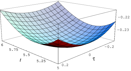
Figure 2: The non-supersymmetric saddle point at the field values given in (19), plotted in the $(t,\tau)$ plane.

3.2 An Example with de-Sitter Turning Points

Having worked through one example in detail let us briefly give another case.

In the presence of non-perturbative effects it is, of course, perfectly possible to obtain de Sitter turning points which are isolated in field space without recourse to any “raising mechanism”. To give an example of this let us consider another example taken from [20].

Retaining the notation in and below (12), the table below summarises the vacua of the heterotic model with superpotential

$$W=8T+6Z+48e^{-S/10}.$$ (21)

As before we only include those ideals which contain extrema.

Ideal	Vacua type	Physical?
$\langle f_{1},f_{2},f_{3},f_{4},f_{5},f_{6}\rangle$	supersymmetric	Yes, AdS saddles
$(\langle\partial V,f_{2},f_{3},f_{4},f_{5},f_{6}\rangle:f_{1}^{\infty})$	partially F-flat	No, $t=0$
$(\langle\partial V,f_{1},f_{2},f_{4},f_{5},f_{6}\rangle:f_{3}^{\infty})$	partially F-flat	No, $z=0$
$(((\langle\partial V,f_{2},f_{4},f_{6}\rangle:f^{\infty}_{1}):f^{\infty}_{3}):f^{\infty}_{5})$	non SUSY	Yes, dS and AdS saddles
$(((((\langle\partial V,f_{5}\rangle:f^{\infty}_{1}):f^{\infty}_{2}):f^{\infty}_{3}):f^{\infty}_{4}):f^{\infty}_{6})$	non SUSY	No, $z\not\in\mathbb{R}$

As an example let us discuss the ideal, $(((\langle\partial V,f_{2},f_{4},f_{6}\rangle:f_{1}^{\infty}):f_{3}^{\infty}):f_{5}^{\infty})$ in the second to last row of the above table. We primary decompose this ideal (thus completing steps 1 and 2) and find four primary ideals, $\mathcal{P}_{1}\ldots\mathcal{P}_{4}$. To illustrate, $\mathcal{P}_{1}$ is

$$\begin{split}\langle&y+1,\quad 4\tau+3\zeta,\quad 18sx-180xy-20t-15z,\quad 2s^{2}-45s+50,\\ &4ts+3zs-117sx+90x,\quad 16tz-12tx-9zx-216x^{2},\\ &64t^{2}+48tz+36z^{2}-2412tx-1809zx+18792x^{2},\\ &4z^{2}s-156zsx+189sx^{2}+120zx-90x^{2},\quad 16z^{3}-804z^{2}x+396tx^{2}+8649zx^{2}-20520x^{3}\rangle.\end{split}$$

Projecting (step 3) onto the pairs $(\sigma,y)$ and $(s,x)$ we find, writing rational approximations to the field values valid to the $10^{-5}$ level,

$$\begin{split}0&=y+1\implies\sigma=10(2n+1)\pi,\quad n\in\mathbb{Z},\\ 0&=2s^{2}-45s+50,\implies s_{1}=\frac{177}{151}\ .\end{split}$$

For the other solution of the quadratic equation in $s$ we find there are no physical solutions. This eliminates the exponentiated variables (step 4). We substitute the above values into $V$ and form the new ideal of derivatives with respect to the remaining variables, returning us to the perturbative algorithm. The relevant term in the saturation expansion is a single primary ideal. It is one dimensional in the variables $\tau,\zeta,t$ and $z$. The physical solutions are

$$\begin{split}0&=4\tau+3\zeta,\\ t&=\frac{1089}{151},\qquad z=\frac{1117}{484},\\ \text{or }t&=\frac{566}{327},\qquad z=\frac{1452}{151}.\end{split}$$ (22)

The following table summaries these results and those following from repeating these steps with the remaining three primary ideals, $\mathcal{P}_{2}$, $\mathcal{P}_{3}$, $\mathcal{P}_{4}$. None of these solutions represent isolated vacua - they each have a flat direction given by $4\tau+3\zeta=0$:

$t$	$z$	$s$	$\sigma$	Vacuum
16.590	22.120	6.564	$10(2n+1)\pi$	de Sitter saddle, $V\simeq 2.10^{-7}$
7.212	2.308	1.172	$10(2n+1)\pi$	AdS saddle, $V\simeq-1.10^{-3}$
1.731	9.616	1.172	$10(2n+1)\pi$	AdS saddle, $V\simeq-1.10^{-3}$

We see then that we do indeed obtain a de Sitter saddle point for this system. Note that although the value of the classical cosmological constant for this turning point is of the order of $10^{-7}$ in the units being used here, and we have approximated the numerical solutions to the dilaton to order $10^{-5}$, this result is not a numerical artifact. We can repeat the calculation at greatly increased precision, say $10^{-12}$ and the values given above persist.

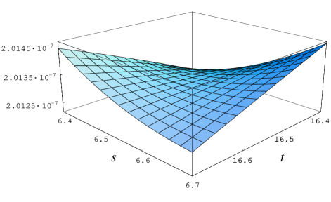
Figure 3: The de Sitter saddle point described in the text, plotted in the $s$, $t$ plane.

3.3 Some IIB Examples

It is a simple matter, using our methods, to show that the KKLT setup [2],

$$W=W_{0}+e^{-cT},\qquad K=-3\log(T+\bar{T}),$$ (23)

has no vacua other than the well-known supersymmetric AdS minimum. We define $f_{1}$ and $f_{2}$ to be the real and imaginary parts of $F_{T}$, and $t$ and $\tau$ to be the real and imaginary parts of $T$. Assuming $c$ and $W_{0}$ are non-zero we find that the ideals $(\langle\partial V,f_{1}\rangle:f_{2}^{\infty})$, $(\langle\partial V,f_{2}\rangle:f_{1}^{\infty})$ and $((\langle\partial V\rangle:f_{1}^{\infty}):f_{2}^{\infty})$ each include the generator $ct+2$ which describes an unphysical vacuum at $ct=-2$. This exhausts the saturation decomposition and thus the supersymmetric vacuum is the only isolated physical extremum.

We now consider a slightly more complicated example where the dilaton is not integrated out.

$$W=W_{0}+aS+e^{-cT},\qquad K=-3\log(T+\bar{T})-\log(S+\bar{S}).$$ (24)

We shall define, in the rest of this subsection, $f_{3}$ and $f_{4}$ to be the real and imaginary parts of $F_{S}$ and $s$ and $\sigma$ to be the real and imaginary parts of $S$. The following table summarizes the vacua of this system (as in earlier examples we have assumed some field values in the computationally expensive final term of the saturation expansion, as shown in the table).

Ideal	Vacua type	Physical Vacua?
$\langle f_{1},f_{2},f_{3},f_{4}\rangle$	supersymmetric	AdS Saddles
$((\langle\partial V,f_{2},f_{4}\rangle:f_{1}^{\infty}):f_{3}^{\infty})$	non SUSY	AdS Saddles
$((((\langle\partial V,t-24,\tau\rangle:f_{1}^{\infty})\ldots:f_{4}^{\infty})$	non SUSY	No

Consider primary decomposing the supersymmetric ideal. For simplicity we assume $c$, $W_{0}$ and $a$ are real and non-zero and so saturate out the monomial $cW_{0}atsxy$, which also removes unphysical solutions. We then find two zero dimensional ideals generated by,

$$\langle\sigma,\quad as-W_{0}\mp x,\quad y\mp 1,\quad ctx\pm 3W_{0}+3x\rangle.$$ (25)

Here $y=e^{-ic\tau}$ and $x=e^{-ct}$. Eliminating all of the variables except $(\tau,y)$ gives the constraint $y\mp 1$ while eliminating to the pair $(t,x)$ gives the final generator of (25).

We must now enumerate the solutions to the transcendental equation given by the final generator of the ideal (25).

$$cte^{-ct}\pm 3W_{0}+3e^{-ct}=0$$ (26)

This is simpler than it may at first appear. Equation (26) is solved, in terms of the Lambert W-function $\mathcal{W}_{n}$, as follows [21]:

$$ct=-3-\mathcal{W}_{n}(\pm 3\,W_{0}\,e^{-3})\ .$$ (27)

We recall the definition of the Lambert W-function as the inverse function to $f(\mathcal{W}_{n})=\mathcal{W}_{n}\exp(\mathcal{W}_{n})$. Equation (27) then represents at most two real solutions for $W_{0}$ real, given by the branches $n=0$ and $-1$ of the Lambert W-function. To proceed, let us choose some values for the parameters: $c=1/10$, and $W_{0}=-10^{-4}$. The only physical solution in (27) is then obtained when we take the positive sign and when $n=-1$. We find $t\simeq 107.314$. In addition, from the second generator in (25), we have $y=1\implies\tau/10=2n\pi$ for $n\in\mathbb{Z}$.

Having eliminated the variables which appear transcendentally we are now in a position to return to the perturbative stage of our method. However, given the simplicity of the ideal (25), we may simply read off the remaining field values in this case.

$$\sigma=0,\quad as\simeq-7.815\times 10^{-5}\ .$$ (28)

We see that in order to have a solution at $s>1$ we need a very small value for $a$. For example, taking $a=-10^{-5}$ we find $s=7.815$. We then obtain an AdS saddle point, not a minimum, with cosmological constant $V\simeq-4.5\times 10^{-16}$, although this turning point is of course Breitenlohner-Freedman stable.

This system also admits non-supersymmetric vacua. The ideal $((\langle\partial V,f_{2},f_{4}\rangle:f_{1}^{\infty}):f_{3}^{\infty})$ may be primary decomposed into four pieces. Two of these pieces require $a=0$ (so that $S$ contributes only to the Kähler potential, not to the superpotential). The corresponding vacua are not isolated as $\sigma$ is a flat direction. We move on to the case $a\not=0$. There are two remaining primary ideals, $\mathcal{P}_{+}$ and $\mathcal{P}_{-}$, which we reproduce below:

$$\begin{split}\mathcal{P}_{+}=\langle&y-1,\quad\sigma,\quad 4c^{2}t^{2}x+2acst+2ctW_{0}+8ctx+7as+W_{0}+x,\\ &2acstx+3a^{2}s^{2}-10ctW_{0}x-4ctx^{2}+7asx-3W_{0}^{2}-5W_{0}x-2x^{2},\\ &4a^{2}cs^{2}t-20c^{2}t^{2}W_{0}x-8c^{2}t^{2}x^{2}-2acstW_{0}+6acstx-7a^{2}s^{2}-6ctW_{0}^{2}\\ &\ -10ctW_{0}x-4ctx^{2}-asW_{0}-asx,\\ &6a^{3}s^{3}-28acstW_{0}x-18acstx^{2}+21a^{2}s^{2}x-4ctW_{0}^{2}x-34ctW_{0}x^{2}-12ctx^{3}\\ &\ -6asW_{0}^{2}-44asW_{0}x-17asx^{2}-5W_{0}^{2}x-7W_{0}x^{2}-2x^{3}\rangle\ .\end{split}$$ (29)

$$\begin{split}\mathcal{P}_{-}=\langle&y+1,\quad\sigma,\quad 4c^{2}t^{2}x-2acst-2ctW_{0}+8ctx-7as-W_{0}+x\\ &2acstx-3a^{2}s^{2}-10ctW_{0}x+4ctx^{2}+7asx+3W_{0}^{2}-5W_{0}x+2x^{2},\\ &4a^{2}cs^{2}t+20c^{2}t^{2}W_{0}x-8c^{2}t^{2}x^{2}-2acstW_{0}-6acstx-7a^{2}s^{2}-6ctW_{0}^{2}\\ &\ +10ctW_{0}x-4ctx^{2}-asW_{0}+asx,\\ &6a^{3}s^{3}+28acstW_{0}x-18acstx^{2}-21a^{2}s^{2}x+4ctW_{0}^{2}x-34ctW_{0}x^{2}+12ctx^{3}\\ &\ -6asW_{0}^{2}+44asW_{0}x-17asx^{2}+5W_{0}^{2}x-7W_{0}x^{2}+2x^{3}\rangle\ .\end{split}$$ (30)

Consider first the ideal $\mathcal{P}_{+}$. Projecting the corresponding variety onto the $(\tau,y)$ plane we find $y=1$. Projecting onto the $(t,x)$ plane and using the definition of $x$ we find the following equation for $t$

$$f_{+}(t) \equiv 4c^{4}t^{4}e^{-2ct}+4c^{3}t^{3}e^{-2ct}-30c^{2}t^{2}W_{0}e^{-ct}-41c^{2}t^{2}e^{-2ct}-9ctW_{0}^{2}-87ctW_{0}e^{-ct}$$

$$-78cte^{-2ct}-18W_{0}^{2}-36W_{0}e^{-ct}-18e^{-2ct}=0.$$

Performing a similar analysis for $\mathcal{P}_{-}$, we find $y=-1$ and

$$f_{-}(t) \equiv 4c^{4}t^{4}e^{-2ct}+4c^{3}t^{3}e^{-2ct}+30c^{2}t^{2}W_{0}e^{-ct}-41c^{2}t^{2}e^{-2ct}-9ctW_{0}^{2}+87ctW_{0}e^{-ct}$$

$$-78cte^{-2ct}-18W_{0}^{2}+36W_{0}e^{-ct}-18e^{-2ct}=0.$$

Let us take the same values of $c$, $W_{0}$ and $a$ ($1/10$, $-10^{-4}$ and $-10^{-5}$ respectively) as for the above analysis of the ideal of supersymmetric vacua. Solving these equations requires use of the numerical step of our algorithm, for which we employ Mathematica. We will look for vacua with $1\leq t\leq 250$ and we start by enumerating the number of vacua in this range. Beginning with $\mathcal{P}_{+}$, we perform the contour integration described in Section 2,

$$\oint\!\mathrm{d}z\,\,\frac{\partial_{z}f_{+}(z)}{f_{+}(z)},$$ (33)

with the ‘radius’ of the contour initially set at $0.1$, so $z=t-0.1i$ on the straight line segment lying below the real axis, for example. This calculation tells us that there are two roots. Having found the number of roots we now use a numerical root finding routine for uni-variate systems to locate them. One root is located at $t_{1}\simeq 35.396\ldots$. We now perform an integral over the circular contour $z=35.396+0.1\exp i\theta$ and find the multiplicity of this root to be one. The second and final root is found at $t_{2}\simeq 133.411$, and is also of multiplicity one. The ideal $\mathcal{P}_{-}$ yields two further roots on following the same procedure. We are now certain to have found all of the solutions for $t$ in the specified range.

Once we have eliminated the transcendental variables in this manner we return to the perturbative algorithm. We find that only the values $y=1$ and $t=t_{1}$ (i.e. one of the roots of the ideal $\mathcal{P}_{+}$) lead to a genuine physical vacuum, which is an AdS saddle point at $\sigma=0$, $s\simeq 16.369$ with $V\simeq-3.6\times 10^{-13}$. This vacuum is not Breitenlohner-Freedman stable.

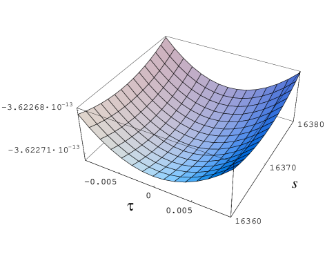
Figure 4: The IIB AdS saddle point at $\tau=0$, $t\simeq 35.396$, $s\simeq 16,369$, $\sigma=0$ plotted in the $\tau,s$ plane

4 Constraints on Flux Parameters

In addition to finding vacua, we can also place powerful constraints on the parameters that arise in flux compactifications. This was done in [11] for the case of perturbative superpotentials. The essential tool here is the elimination of variables in an ideal, which we have already discussed in the context of projection onto the space spanned by the dummy and exponentiated variables in the previous section.

Given some Kähler and superpotential we take the set of parameters which are present, call them $a_{\alpha}$, as variables and consider our initial ideal, $\langle\partial V\rangle$ or part of its saturation decomposition, as living in the ring $\mathbb{C}[m_{i},\mu_{i},n_{a},\nu_{a},x_{a},y_{a},a_{\alpha}]$. We then eliminate the field variables $m_{i},\mu_{i},n_{a},\nu_{a},x_{a},y_{a}$. Algebraically this is the intersection of our ideal with the ring $\mathbb{C}[m_{i},\mu_{i},n_{a},\nu_{a},x_{a},y_{a}]$. Geometrically, this is the projection of our ideal onto the surface where the field variables and their exponentials vanish. The elements of the resulting ideal then represent necessary constraints on the parameters for extrema to exist. These, of course, apply in addition to any constraint already imposed on the system by other considerations.

As a simple example, consider the following Kähler and superpotentials obtained from the heterotic string compactified on generalised half-flat manifolds in the presence of flux and gaugino condensation [20]:

$$\begin{split}W&=i(\xi+ieT)+(\epsilon+ipT)Z+\frac{i}{2}(\mu+iqT)Z^{2}+\lambda e^{-cS},\\ K&=-3\log(T+\bar{T})-3\log(Z+\bar{Z})-\log(S+\bar{S})\ .\end{split}$$ (34)

In the notation of our general discussion we would write $\{M_{i}=m_{i}+i\mu_{i}\}=\{Z=z+i\zeta,T=t+i\tau\}$ and $\{N=n+i\nu\}=\{S=s+i\sigma\}$.

In this system, the flux parameters obey the constraint,

$$\epsilon q-\mu p=0,$$ (35)

which follows from the Bianchi identity in the case of a ‘standard embedding’ [20].

To demonstrate, let us consider the supersymmetric vacua of this system. The properties of the supersymmetric vacua are determined by the ideal generated by the real and imaginary parts of the F-terms and the constraint (35), $\langle f_{1},f_{2},f_{3},f_{4},f_{5},f_{6},-\epsilon q+\mu p\rangle$, in the ring $\mathbb{C}[\xi,e,\epsilon,p,\mu,q,\lambda,c,s,t,z,\sigma,\tau,\zeta]$. Here $f_{1}$ and $f_{2}$ are the real and imaginary parts of $F_{T}$, $f_{3}$ and $f_{4}$ the real and imaginary parts of $F_{Z}$ and $f_{5}$ and $f_{6}$ the real and imaginary parts of $F_{S}$. In addition we are making our habitual complexification of the field, and now parameter, space.

One question we could ask is, given some physical constraints that we wish the field values to obey in vacuum, what constraints are necessary amongst the parameters for the existence of a supersymmetric vacuum of that form? Looking at the strengths of the gravitational and gauge interactions, and insisting on a vanishing theta term for the gauge fields, one might choose a set of field values of the form $s=24,t=1,\sigma=0$. These physical requirements can be enforced by including appropriate extra generators in our initial ideal. In this case, this would correspond to taking the ideal $\langle f_{1},f_{2},f_{3},f_{4},f_{5},f_{6},-\epsilon q+\mu p,s-24,t-1,\sigma\rangle$. We then eliminate all of the field variables using a Gröbner basis calculation as described above. The result is the following set of constraints amongst the parameters.

$$\begin{array}[]{rcl}0&=&\mu p-q\epsilon\\ 0&=&pq\xi-eq\epsilon\\ 0&=&p^{2}\xi-ep\epsilon\\ 0&=&96cp\xi-96ce\epsilon-p\xi+e\epsilon\\ 0&=&e\mu q-q^{2}\xi\\ 0&=&e^{2}\mu-eq\xi\\ 0&=&96ce\mu-96cq\xi-e\mu+q\xi\ .\end{array}$$ (36)

Thus, if we are looking for supersymmetric vacua in compactifications of Heterotic on generalised half-flat manifolds with gaugino condensation in which the interaction strengths are physical and the theta angle is zero, then the above constraints among the parameters in $W$ must hold.

We can in fact do even better. By using various pieces of the methodology espoused in this paper, and in [11], we can make other demands of the system. For example, we may require that none of the parameters are zero (so that all terms in (34) contribute). To achieve this we simply take the ideal generated by the right hand sides in (36) and saturate out the polynomial which is the product of the parameters, $ec\mu\xi pq\epsilon$. Given the geometrical interpretation of saturation, as discussed in Section 2, this then gives us equations for the parts of the variety of constraints in parameter space for which none of the parameters vanish.

$$\begin{array}[]{rcl}0&=&p\xi-e\epsilon\\ 0&=&\mu p-q\epsilon\\ 0&=&e\mu-q\xi\ .\end{array}$$ (37)

One of these three constraints is redundant and another is simply that which follows from the Bianchi identity (35). This thus leaves us with a single additional simple constraint on the parameters, $e\mu-q\xi=0$.

Such constraints are clearly of great utility in searching for vacua of these systems - whether using the methods presented in this paper or more conventional techniques. A quick Gröbner basis calculation can cut out huge swathes from the parameter space which needs to be searched.

5 Conclusions

We have shown that the algebro-geometric techniques, advocated in [11], for finding vacua of supergravity systems can be modified to incorporate the effects of non-perturbative contributions to the superpotential. While the modification required does introduce a numerical element to our method, much of the information that can be obtained remains analytic. In particular, we can analytically prove that we do not miss any vacua due to this numerical step.

While not a universal cure to the problems of finding vacua in string phenomenology systems, these methods do render the process significantly less time consuming and painful. Many of the vacua which spontaneously break supersymmetry and may be found with our methods are very unlikely to be found with more conventional techniques. In many cases the techniques espoused here represent the most powerful tool currently available in searching for vacua in a given theory.

The algorithmic nature of the methods presented in this paper and in [11] is important. It means that it is conceivable to create a ‘black box’ package to which one feeds information such as a Kähler and Superpotential, ranges for the parameters of interest and physical requirements on the vacua to be found. The program would then simply cycle through the specified parameter range, outputting any vacua present of the type desired. A user specified time constraint would impose an upper limit on how far along the saturation expansion one could reach in each case. It is the intention of the authors to make such a black box available as the next step in this program of research.

References

- [1] S. B. Giddings, S. Kachru and J. Polchinski, “Hierarchies from fluxes in string compactifications,” Phys. Rev. D 66 (2002) 106006 [arXiv:hep-th/0105097].
- [2] S. Kachru, R. Kallosh, A. Linde and S. P. Trivedi, “De Sitter vacua in string theory,” Phys. Rev. D 68 (2003) 046005 [arXiv:hep-th/0301240].
- [3] V. Balasubramanian, P. Berglund, J. P. Conlon and F. Quevedo, “Systematics of moduli stabilisation in Calabi-Yau flux compactifications,” JHEP 0503, 007 (2005) [arXiv:hep-th/0502058].
- [4] M. Grana, “Flux compactifications in string theory: A comprehensive review,” Phys. Rept. 423, 91 (2006) [arXiv:hep-th/0509003].
- [5] E. I. Buchbinder and B. A. Ovrut, “Vacuum stability in heterotic M-theory,” Phys. Rev. D 69, 086010 (2004) [arXiv:hep-th/0310112].
- [6] J. Gray, A. Lukas and B. Ovrut, “Perturbative anti-brane potentials in heterotic M-theory,” arXiv:hep-th/0701025.
- [7] B. de Carlos, A. Lukas and S. Morris, “Non-perturbative vacua for M-theory on G(2) manifolds,” JHEP 0412, 018 (2004) [arXiv:hep-th/0409255].
- [8] B. Acharya, K. Bobkov, G. Kane, P. Kumar and D. Vaman, “An M theory solution to the hierarchy problem,” Phys. Rev. Lett. 97, 191601 (2006) [arXiv:hep-th/0606262].
- [9] B. S. Acharya, K. Bobkov, G. L. Kane, P. Kumar and J. Shao, “Explaining the electroweak scale and stabilizing moduli in M theory,” arXiv:hep-th/0701034.
- [10] A. Micu, E. Palti and G. Tasinato, “Towards Minkowski vacua in type II string compactifications,” arXiv:hep-th/0701173.
- [11] J. Gray, Y. H. He and A. Lukas, “Algorithmic algebraic geometry and flux vacua,” JHEP 0609, 031 (2006) [arXiv:hep-th/0606122].
-
[12]
J. Gray, Y. H. He, V. Jejjala and B. D. Nelson,
“Exploring the vacuum geometry of N = 1 gauge theories,”
Nucl. Phys. B 750, 1 (2006)
[arXiv:hep-th/0604208].
J. Gray, Y. H. He, V. Jejjala and B. D. Nelson, “Vacuum geometry and the search for new physics,” Phys. Lett. B 638, 253 (2006) [arXiv:hep-th/0511062]. - [13] J. Distler and U. Varadarajan, “Random polynomials and the friendly landscape,” arXiv:hep-th/0507090.
- [14] A. Strominger, “Massless black holes and conifolds in string theory,” Nucl. Phys. B 451, 96 (1995) [arXiv:hep-th/9504090].
- [15] D. Grayson and M. Stillman, “Macaulay 2, a software system for research in algebraic geometry.” Available at http://www.math.uiuc.edu/Macaulay2/
- [16] G.-M. Greuel, G. Pfister, and H. Schönemann, ”Singular: A Computer Algebra System for Polynomial Computations,” Centre for Computer Algebra, University of Kaiserslautern (2001). Available at http://www.singular.uni-kl.de/
- [17] P. Breitenlohner and D. Z. Freedman, “Positive Energy In Anti-De Sitter Backgrounds And Gauged Extended Supergravity,” Phys. Lett. B 115, 197 (1982).
- [18] Mathematica Version 5.2, Wolfram Research, Inc. 2005.
- [19] Maple 10.06, Waterloo Maple Inc. (Maplesoft). 2006.
-
[20]
S. Gurrieri, A. Lukas and A. Micu,
“Heterotic on half-flat,”
Phys. Rev. D 70, 126009 (2004)
[arXiv:hep-th/0408121].
B. de Carlos, S. Gurrieri, A. Lukas and A. Micu, “Moduli stabilisation in heterotic string compactifications,” JHEP 0603, 005 (2006) [arXiv:hep-th/0507173]. - [21] R. M. Corless et al, “On the Lambert W function” Adv. Comp. Maths 5 (1996) 329
- [22] M. Gomez-Reino and C. A. Scrucca, “Locally stable non-supersymmetric Minkowski vacua in supergravity,” JHEP 0605 (2006) 015 [arXiv:hep-th/0602246].
- [23] M. Gomez-Reino and C. A. Scrucca, “Constraints for the existence of flat and stable non-supersymmetric vacua in supergravity,” JHEP 0609 (2006) 008 [arXiv:hep-th/0606273].
- [24] M. Soroush, “Constraints on meta-stable de Sitter flux vacua,” [arXiv:hep-th/0702204].