Noncommutative QED corrections to process $e^{+}e^{-}\rightarrow\mu^{+}\mu^{-}\gamma$ at linear collider energies

Abstract

The cross section for process $e^{+}e^{-}\rightarrow\mu^{+}\mu^{-}\gamma$ in the framework of noncommutative quantum electrodynamics(NC QED) is studied. It is shown that the NC correction of scattering sections is not monotonous enhancement with total energy of colliding electrons, but there is an optimal collision energy to get the greatest NC correction. Moreover, there is a linear relation between NC QED scale energy and the optimal collision energy. The experimental methods to improve the precision of determining NC effects are discussed, because this process is an ${\cal O}(\alpha^{3})$ NC QED process, high precision tests are necessary.

I INTRODUCTION

The noncommutativity of space-time was firstly introduced by SnyderSnyder47 . It has been revived recently with the emergence of noncommutative quantum field theories (NC QFT) from string theories Connes98 ; Douglas98 ; SW99 , which has attracted much attention Sheikh-Jabbari99 ; Martin99 ; Ishibashi00 ; Ya00 ; Petriello01 ; Carroll01 ; Seiberg00 ; Anisimov02 ; Chaichian05 . It was generally assumed that predictions of string theory and NC effects can only be examined at Plank scale or the grand unification scale. However, given the possibility Witten96 ; Hewett01 that the onset of string effects is at the  TeV  scale, and that gravity becomes strong at a few  TeV, it is feasible that NC effects could also show up at a few  TeV.

In Refs.Hewett01 ; Kamoshita ; Arfaei00 ; Baek01 ; Godfrey02 ; Abbiendi03 ; sheng ; Alberto05 , several NC Quantum Electrodynamics (QED) processes in $e^{+}e^{-}$ collisions have been studied. However, the NC radiative effects in electron-positron annihilations have not been studied before. It is necessary to include the radiative effects in considering the NC effects for those reactions, because the radiative corrections due to emission of hard photons become more and more important as $e^{+}e^{-}$ collision energy increasesNuovo ; petriello03 . A linear relation between the fundamental NC scale $\Lambda_{NC}$ and the optimal collision energy at which NC correction of scattering section arrives at the maximum, for Möller scattering and Bhabha Scattering was found in Ref.sheng . It is interesting to explore the availability of this linear relation for reaction $e^{+}e^{-}\rightarrow\mu^{+}\mu^{-}\gamma$, because there are three photon self-interactions for reaction $e^{+}e^{-}\rightarrow\mu^{+}\mu^{-}\gamma$ in the NC QED, which is forbidden in conventional QED.

The essential idea of NC QED is a generalization of QED based on the usual d-dimensional space, $R^{d}$, associated with commuting space-time coordinates to one which is based on non-commuting, $R^{d}_{\theta}$. In such a space the conventional coordinates are replaced by operators which no longer commute each other. The NC space-time can be realized by the coordinate operators satisfyingSW99 ; Hewett01 ; Kamoshita

$$[\hat{X}_{\mu},\hat{X}_{\nu}]=i\theta_{\mu\nu}=\frac{ic_{\mu\nu}}{\Lambda_{NC}^{2}},$$ (1)

where $\theta_{\mu\nu}$ is a constant antisymmetric matrix, having dimension of $(length)^{2}$ = $(mass)^{-2}$, and $c_{\mu\nu}$ is a real antisymmetric matrix, whose dimensionless elements are presumably of order unity. In the last equality of eq.(1), we have parameterized the effect in terms of an overall scale $\Lambda_{NC}^{2}$, which characterizes the threshold where NC effects become relevant, its role can be compared to that of $\hbar$ in conventional Quantum Mechanics, which represents the level of non-commutativity between coordinates and momenta. The existence of a finite $\Lambda_{NC}$ represents existence of a fundamental space-time distance below which the space-time coordinates become fuzzy.

When the particle energy is near or higher than $\Lambda_{NC}$, we have to replace conventional Quantum field theories (QFT) by NC QFT which is based on noncommutative space-time. So the determination of $\Lambda_{NC}$ is important in NC QFT. Its lower bound has been found to be $\Lambda_{NC}>100GeV$ Chaichian so that the result of Lamb shift is consistent with the ordinary quantum mechanics.

NC QFT can be presented in terms of conventional commuting QFT through the application of Weyl-Moyal correspondenceSheikh-Jabbari99 :

$$\hat{\Phi}(\hat{X})\longleftrightarrow\Phi(x),$$ (2)

$$\hat{\Phi}_{1}(\hat{X})\hat{\Phi}_{2}(\hat{X})\longleftrightarrow\Phi_{1}(x)\star\Phi_{2}(x),$$ (3)

where $\Phi$ represents quantum fields with $\hat{X}$ being the set of non-commuting coordinates and $x$ corresponding to the commuting set, and the Moyal $\star$-product is defined by

$$(f\star g)(x)=exp\left(\frac{1}{2}\theta_{\mu\nu}\partial_{x^{\mu}}\partial_{y^{\nu}}\right)f(x)g(y)|_{y=x}.$$ (4)

Thus the Lagrangians with set of non-commuting coordinates will correspond to those with commuting set, but the ordinary products of all fields in the Lagrangians of their commutative counterparts should be replaced by the Moyal $\star$-products.

We can get the NC QED Lagrangian by using above recipe as

$${\cal L}=\frac{1}{2}i(\bar{\psi}\star\gamma^{\mu}D_{\mu}\psi-(D_{\mu}\bar{\psi})\star\gamma^{\mu}\psi)-m\bar{\psi}\star\psi-\frac{1}{4}F_{\mu\nu}\star F^{\mu\nu},$$ (5)

where $D_{\mu}\psi=\partial_{\mu}\psi-ieA_{\mu}\star\psi$,$~{}~{}(D_{\mu}\bar{\psi})=\partial_{\mu}\bar{\psi}+ie\bar{\psi}\star A_{\mu}$, and $~{}~{}F_{\mu\nu}=\partial_{\mu}A_{\nu}-\partial_{\nu}A_{\mu}-ie(A_{\mu}\star A_{\nu}-A_{\nu}\star A_{\mu})$. This Lagrangian can be used to obtain the Feynman rules for perturbation calculations. The propagators for the free fermions and gauge fields of NC QED are the same as that in the case of ordinary QED. But for interaction terms, every interaction vertex has a phase factor $exp(ip_{1}^{\mu}\theta_{\mu\nu}p_{2}^{\nu}/2)$ correction depending on in and out 4-momentum. Moreover, there are cubic and quadric interaction vertices for the gauge field besides the usual vertices found in ordinary QED. The matrix $\theta_{\mu\nu}$ can be decomposed into two independent parts Hewett01 ; Kamoshita : electric-like components $\bf{\theta}_{E}$ $=$ $(\theta_{01},\theta_{02},\theta_{03})$ and magnetic-like components $\bf{\theta}_{B}$ $=$ $(\theta_{23},\theta_{31},\theta_{12})$. $\bf{\theta}_{E}$ and $\bf{\theta}_{B}$ can be considered as 3-vectors which define two unique directions in space. The characteristic properties of NC QED may thus be observed as direction-dependent deviations from the predictions of QED.

In this paper, we adopt the spirit of Ref.Hewett01 to consider the possibility that NC scale energy $\Lambda_{NC}$ is near the  TeV  scale, and study the scattering process $e^{+}e^{-}\rightarrow\mu^{+}\mu^{-}\gamma$ in NC QED to establish the relation for NC correction of scattering section versus collision energy, and then to establish the relation between NC scale $\Lambda_{NC}$ and the optimal collision energy. Finally, the experimental methods to determine the NC scale energy $\Lambda_{NC}$ and to improve the precision of determining NC effects will be discussed, because this process is an ${\cal O}(\alpha^{3})$ NC QED process, high precision tests has to be necessary.

II NC QED SCATTERING AMPLITUDES

Shown in Fig.1 are the five Feynman diagrams, which are the lowest tree level contributions to the process.

Figure 1: Feynman graph of scattering process $e^{+}e^{-}\rightarrow\mu^{+}\mu^{-}\gamma$

Comparing with ordinary QED, we have one more Feynman graph, namely Fig. $M_{5}$. This is due to the coupling of three photons in noncommutative space-time. Using the Feynman rules in Ref.Sheikh-Jabbari99 and the Dirac equation, we get the corresponding scattering amplitude as following

$$\begin{array}[]{ll}M_{1}=&\frac{ig^{3}\varepsilon^{*}_{\sigma}(k)}{(p^{\prime}+q^{\prime})^{2}(2q\cdot k)}\bar{v}^{r_{1}}(q)\gamma^{\sigma}(-q\!\!\!/+k\!\!\!/+m)\gamma^{\mu}u^{r_{2}}(p)\bar{u}^{s_{1}}(p^{\prime})\gamma_{\mu}v^{s_{2}}(q^{\prime})\\ \\ &e^{i(p+q)\theta(-q+k)/2-iq^{\prime}\theta p^{\prime}/2},\end{array}$$ (6)

$$\begin{array}[]{ll}M_{2}=&\frac{ig^{3}\varepsilon^{*}_{\sigma}(k)}{(p^{\prime}+q^{\prime})^{2}(2p\cdot k)}\bar{v}^{r_{1}}(q)\gamma^{\mu}(p\,\!\!\!\!/-k\!\!\!/+m)\gamma^{\sigma}u^{r_{2}}(p)\bar{u}^{s_{1}}(p^{\prime})\gamma_{\mu}v^{s_{2}}(q^{\prime})\\ \\ &e^{i(p+q)\theta(p-k)/2-iq^{\prime}\theta p^{\prime}/2},\end{array}$$ (7)

$$\begin{array}[]{ll}M_{3}=&\frac{-ig^{3}\varepsilon^{*}_{\sigma}(k)}{(p+q)^{2}(2p^{\prime}\cdot k)}\bar{v}^{r_{1}}(q)\gamma_{\mu}u^{r_{2}}(p)\bar{u}^{s_{1}}(p^{\prime})\gamma^{\sigma}(p\,\!\!\!\!/\,^{\prime}+k\!\!\!/+\mu)\gamma^{\mu}v^{s_{2}}(q^{\prime})\\ \\ &e^{i(p^{\prime}+k)\theta(p^{\prime}+q^{\prime})/2-ip\theta q/2},\end{array}$$ (8)

$$\begin{array}[]{ll}M_{4}=&\frac{-ig^{3}\varepsilon^{*}_{\sigma}(k)}{(p+q)^{2}(2q^{\prime}\cdot k)}\bar{v}^{r_{1}}(q)\gamma_{\mu}u^{r_{2}}(p)\bar{u}^{s_{1}}(p^{\prime})\gamma^{\mu}(-q\!\!\!/\,^{\prime}-k\!\!\!/+\mu)\gamma^{\sigma}v^{s_{2}}(q^{\prime})\\ \\ &e^{i(-q^{\prime}-k)\theta(p^{\prime}+q^{\prime})/2-ip\theta q/2},\end{array}$$ (9)

$$\begin{array}[]{ll}M_{5}=&\frac{-2g^{3}\sin(k\theta(p+q)/2)\varepsilon^{*}_{\sigma}(k)}{(p+q)^{2}(p^{\prime}+q^{\prime})^{2}}\bar{v}^{r_{1}}(q)\gamma^{\mu}u^{r_{2}}(p)\left[(-p-q-p^{\prime}-q^{\prime})^{\sigma}g_{\mu\nu}+\left(p^{\prime}\right.\right.\\ \\ &\left.\left.+q^{\prime}-k\right)_{\mu}g^{\sigma}_{\mu}+(k+p+q)_{\nu}g^{\sigma}_{\mu}\right]\bar{u}^{s_{1}}(p^{\prime})\gamma^{\nu}v^{s_{2}}(q^{\prime})e^{-i(p\theta q+q^{\prime}\theta p^{\prime})/2},\end{array}$$ (10)

here $p$, $q$, $p^{\prime}$, $q^{\prime}$ and $k$ are four momentums of electron, positron, muon, anti-muon and photon, respectively; $r_{1}$, $r_{2}$, $s_{1}$, $s_{2}$ are spin indices of corresponding particle, respectively; $m$, $\mu$ are masses of the electron and the muon, respectively.

III SCATTERING CROSS SECTION

The cross section for process $e^{+}e^{-}\rightarrow\mu^{+}\mu^{-}\gamma$ is

$$\sigma=\frac{1}{16w^{2}v}\frac{1}{(2\pi)^{5}}\int|M(p,q\rightarrow p^{\prime},q^{\prime},k)|^{2}(2\pi)^{4}\delta^{(4)}(p+q-p^{\prime}-q^{\prime}-k)\frac{d\mathbf{p^{\prime}}}{p^{\prime}_{0}}\frac{d\mathbf{q^{\prime}}}{q^{\prime}_{0}}\frac{d\mathbf{k}}{k_{0}},$$ (11)

where $p^{\prime}_{0}$, $q^{\prime}_{0}$, $k_{0}$ are energies of outgoing particles respectively, $v$ is the velocity of incident electron, which is given by $v=(1-4m^{2}/w^{2})^{1/2}$. In the center-of-mass system C $(\mathbf{p}+\mathbf{q}=0)$, the total energy of colliding electron-positron beams is $w^{2}=(p+q)^{2}=4E^{2}$, where $E$ is the energy of each of the initial particles, the photon energy $k_{0}$ may vary from a lower limit $\epsilon$ to an upper limit $(w^{2}-4\mu^{2})/2w$ which is determined by the kinematics. The limit $\epsilon$ will in practice be identified with the soft-photon cut-off.

We integrate the cross-section $d\sigma$ over $d\mathbf{p^{\prime}}$ and $d\mathbf{q^{\prime}}$ in the system $C^{\prime}$ in which the center-of-mass of the muons is at rest so that $\mathbf{p^{\prime}}+\mathbf{q^{\prime}}=\mathbf{p}+\mathbf{q}-\mathbf{k}=\mathbf{0}$. The system $C^{\prime}$ is determined when the vector $\mathbf{k}$ in the system $C$ is fixed. Its z-axis is along the orientation of $\mathbf{k}$, the vectors $\mathbf{p}$, $\bf{q}$, $\bf{k}$ are located in the plane $xoz$, the angles between $\bf{p^{\prime}}$ and $\bf{p}$ or $\bf{k}$ are $\tilde{\theta}$ or $\tilde{\gamma}$, the azimuth angle of line $\bf{p^{\prime}}$ is $\tilde{\varphi}$, the angle between vector $\bf{p}$ and $\bf{k}$ is $\tilde{\alpha}$ (see Fig. 2). The integration with respect to $\bf{p^{\prime}}$ and $\bf{q^{\prime}}$ can be converted into integration with respect to $\tilde{\gamma}$, $\tilde{\varphi}$.

Figure 2: The $C^{\prime}$-system in which the center-of-mass of muons is at rest

Then differential cross section is,

$$\frac{d\sigma}{d\mathbf{k}}=\frac{\tilde{v}}{32w^{2}v(2\pi)^{5}k_{0}}\left.\int\limits_{-1}^{1}d\cos\tilde{\gamma}\int\limits_{0}^{2\pi}d\tilde{\varphi}|M(p,q\rightarrow p^{\prime},q^{\prime},k)|^{2}\right|_{p+q-p^{\prime}-q^{\prime}-k=0},$$ (12)

here $\tilde{v}=(1-4\mu^{2}/(p^{\prime}+q^{\prime})^{2})^{1/2}$ is the velocity of muon.

In the C-system, the total cross-section $\sigma$, for the emission of photons whose energy $k_{0}$ varies from $\epsilon$ to $k_{0max}$, is given by

$$\sigma=\int\limits_{\epsilon}^{k_{0max}}\frac{d\sigma}{dk_{0}}dk_{0}=\int\limits_{\epsilon}^{k_{0max}}dk_{0}\int\frac{d\sigma}{d\bf{k}}d\Omega(\bf{k}).$$ (13)

IV NC CORRECTION AND NUMERICAL ANALYSIS

After all the integration, we obtain the following expression of cross-section,

$$\sigma=\sigma_{QED}+(\Delta\sigma)_{NC}.$$ (14)

The first term is the usual QED cross section

$$\sigma_{QED}=\int\limits_{\epsilon}^{k_{0max}}dk_{0}\left(\frac{\left((1-v^{2})w^{2}+2\rho^{2}\right)\gamma_{0}+4{k_{0}}^{2}\gamma_{1}}{\left(3-v^{2}\right)\rho^{2}k_{0}}+\frac{\left((1-\tilde{v}^{2})\frac{\rho^{4}}{w^{2}}+2\rho^{2}\right)\gamma_{0}^{\prime}+4{k_{0}}^{2}\gamma_{1}^{\prime}}{\left(3-\tilde{v}^{2}\right)w^{2}k_{0}}\right)\sigma_{0};$$ (15)

with

$$\sigma_{0}=\frac{1}{3}\frac{\pi\alpha^{2}}{w^{2}}\frac{\tilde{v}}{v}(3-v^{2})(3-\tilde{v}^{2}),$$ (16)

$$\begin{array}[]{l}\gamma_{0}=\frac{2\alpha}{\pi}\left(-1+\frac{1+v^{2}}{2v}\ln\frac{1+v}{1-v}\right),\\ \\ \gamma_{1}=\frac{2\alpha}{\pi}\left(-1+\frac{1}{v}\ln\frac{1+v}{1-v}\right),\\ \\ {\gamma_{0}}^{\prime}=\frac{2\alpha}{\pi}\left(-1+\frac{1+\tilde{v}^{2}}{2\tilde{v}}\ln\frac{1+\tilde{v}}{1-\tilde{v}}\right),\\ \\ {\gamma_{1}}^{\prime}=\frac{2\alpha}{\pi}\left(-1+\frac{1}{\tilde{v}}\ln\frac{1+\tilde{v}}{1-\tilde{v}}\right),\end{array}$$ (17)

here $\alpha$ is the fine structure constant.

The second term is the NC correction defined as the difference between NC QED cross section and commutative QED cross section

$$(\Delta\sigma)_{NC}=2\alpha^{3}\int\limits_{-1}^{1}dz\int\limits_{0}^{2\pi}d\phi\int\limits_{\epsilon}^{k_{0max}}dk_{0}\frac{\tilde{v}}{v}\frac{k_{0}}{w^{4}\rho^{2}}\sin^{2}\frac{k\theta(p+q)}{2}f(w,k_{0},z),$$ (18)

where

$$\sin^{2}\frac{k\theta(p+q)}{2}=\sin^{2}[\frac{-1}{2\Lambda_{NC}^{2}}wk_{0}(c_{01}\sin\gamma\cos\phi+c_{02}\sin\gamma\sin\phi+c_{03}\cos\gamma)],$$ (19)

and $\gamma$, $\phi$ are the polar angle and azimuth angle of photon in C-system, and

$$\begin{array}[]{l}f(w,k_{0},z)=\frac{1}{8\pi w^{2}k_{0}^{2}}\left[-\frac{16w^{4}k_{0}^{2}x}{3(1-vz)}-8w^{2}{\rho}^{4}-4Bw^{2}{\rho}^{2}\left(w^{2}+{\rho}^{2}\right)\right.\\ \\ +y\left(w^{6}-2w^{4}{\rho}^{2}+5w^{2}{\rho}^{4}-2{\rho}^{6}\right)+2Bw^{2}{\rho}^{2}\left(w^{2}+{\rho}^{2}\right)\left(x+y\right)+\frac{4}{3}x\left(w^{2}+{\rho}^{2}\right)\left(w^{4}+{\rho}^{4}\right)\\ \\ +\left(1-vz\right){\rho}^{2}\left(4Bw^{2}{\rho}^{2}-2w^{2}\left(w^{2}-3{\rho}^{2}\right)-\frac{2}{3}x{\rho}^{2}\left(3Bw^{2}+3w^{2}+{\rho}^{2}\right)\right)\\ \\ +xy\left(\frac{4w^{2}\left(w^{4}-{\rho}^{4}\right)}{3\left(1-v^{2}z^{2}\right)}-3Bw^{2}{\rho}^{4}-\frac{w^{8}+2w^{6}{\rho}^{2}-2w^{4}{\rho}^{4}+12w^{2}{\rho}^{6}-{\rho}^{8}}{3{\rho}^{2}}+w^{2}{\rho}^{2}\frac{3B\left(w^{2}+{\rho}^{2}\right)+4\left(w^{2}+2{\rho}^{2}\right)}{3(1+vz)}\right)\\ \\ +\frac{24w^{2}{\rho}^{4}+12Bw^{2}{\rho}^{2}\left(w^{2}+{\rho}^{2}\right)-6y\left(2w^{2}{\rho}^{4}+Bw^{2}{\rho}^{2}\left(w^{2}+{\rho}^{2}\right)\right)-x\left(6Bw^{2}{\rho}^{2}\left(w^{2}+{\rho}^{2}\right)+4w^{2}\left(w^{4}+3{\rho}^{4}\right)\right)}{3(1+vz)}\\ \\ +\left(1-v^{2}z^{2}\right)\left(-w^{6}+4w^{4}{\rho}^{2}-11w^{2}{\rho}^{4}+10{\rho}^{6}+2B{\rho}^{2}\left(w^{4}-5w^{2}{\rho}^{2}+2{\rho}^{4}\right)\right)\\ \\ +\left.x\left(1-v^{2}z^{2}\right)\left(-B{\rho}^{2}\left(2w^{4}-7w^{2}{\rho}^{2}+2{\rho}^{4}\right)+\frac{5w^{8}-27w^{6}{\rho}^{2}+57w^{4}{\rho}^{4}-13w^{2}{\rho}^{6}-6{\rho}^{8}}{6w^{2}}\right)\right].\end{array}$$ (20)

Here $x=3-\tilde{v}^{2}$, $y=3-v^{2}$, $z=\cos\gamma$, $B=\frac{1}{\tilde{v}}\ln\frac{1-{\tilde{v}}}{1+{\tilde{v}}}$, and $\rho^{2}=w^{2}-2\,w\,k_{0}$.

When $\theta\rightarrow 0$, the total cross-section reduces to the ordinary QED result.

IV.1 THE MATRIX $\theta_{\mu\nu}$ IN THE LABORATORY SYSTEM

From the eq.(19), we find that the process $e^{+}e^{-}\rightarrow\mu^{+}\mu^{-}\gamma$ is sensitive only to $\bf{\theta}_{E}$, but not to $\bf{\theta}_{B}$ at tree level. Here $\bf{\theta}_{E}$ is defined as

$${\bf\theta_{E}}=\frac{1}{\Lambda_{NC}^{2}}{\bf c_{E}}=\frac{1}{\Lambda_{NC}^{2}}(c_{01},c_{02},c_{03}),$$ (21)

where $\Lambda_{NC}=1/\sqrt{|\bf{\theta}_{E}|}$ and $c_{0i}$ are components of the unit vector $\bf{c}_{E}$ pointing to the unique direction in the primary coordinate system. In the general case, $\sin^{2}\frac{k\theta(p+q)}{2}$ depends not only on the photon polar angle $\gamma$, but also on the azimuthal angle $\phi$. This is a signature of the anisotropy of space-time which is inherent in noncommutative geometry. In the special case $(c_{01}=c_{02}=0)$, the $\bf{\theta}_{E}$ is independence of $\phi$.

It would be natural to assume that the unique direction $\bf{c}_{E}$ is fixed to some larger structure in space, e.g., the frame of the cosmic microwave background which could be taken as primary frame. In the Lab coordinate system on Earth, $\bf{c}_{E}$ will change as the Earth rotates and as the orientation of the Earth’s rotation axis changes due to the movement of the galaxy or the solar system with respect to the primary frame. We assume that the latter movement is sufficiently slow, the rotation of the Earth is only the relevant motion in the time scale of the experiment.

In the primary frame, the unit vector $\bf{c}_{E}^{0}$ is specified by two parameters, the polar angle $\eta$ and the azimuthal angle $\xi$Kamoshita :

$$\bf{c}_{E}^{0}=\left(\begin{array}[]{c}s_{\eta}c_{\xi}\\ s_{\eta}s_{\xi}\\ c_{\eta}\end{array}\right),$$ (22)

where $s_{\eta}\equiv\sin\eta$, $c_{\xi}\equiv\cos\xi$ and so on.

Elements of the vector $\bf{c}_{E}$ in the local coordinate system (x, y, z) are obtained by successive rotations of the coordinate axes:

$$\begin{array}[]{ll}\bf{c}_{E}&=R_{y}(\beta)R_{z}(-\pi/2)R_{y}(-\delta)R_{z}(\zeta)\cdot\bf{c}_{E}^{0}\\ \\ &=\left(\begin{array}[]{c}s_{\beta}s_{\delta}\\ c_{\delta}\\ -c_{\beta}s_{\delta}\end{array}\right)s_{\eta}\cos(\zeta-\xi)+\left(\begin{array}[]{c}c_{\beta}\\ 0\\ s_{\beta}\end{array}\right)s_{\eta}\sin(\zeta-\xi)+\left(\begin{array}[]{c}-s_{\beta}c_{\delta}\\ s_{\delta}\\ c_{\beta}c_{\delta}\end{array}\right)c_{\eta},\end{array}$$ (23)

here the angle $\delta$ is the latitude of the experiment location, $\beta$ is the angle between the z-axis and the direction of north, $\zeta$ is a time-dependent azimuthal angle of the experiment site, given byAbbiendi03 :

$$\zeta(t)=\omega t,$$ (24)

where $\omega=2\pi/T_{sd}$ with sidereal day $T_{sd}$.

So the $c_{0i}$ will vary with experiment site, i.e., with values of $\beta$, $\delta$ and $\eta$, and the variation of $c_{0i}$ with time is decided by $\zeta-\xi$. When $\beta=\delta=\eta=0$, we get $c_{03}=1$, and $c_{01}=c_{02}=0$.

IV.2 NUMERICAL ANALYSIS

Now we consider NC correction to the total cross-section for the process $e^{+}e^{-}\rightarrow\mu^{+}\mu^{-}\gamma$ by numerical integration. The energy of the photon varies from $\epsilon=0.01\mu$ to $k_{0max}=2w/5$ in our case. The relation curve between cross-section $\sigma$ and collision energy $w$ is shown in Fig. 3. The cross-section of this process decreases with collision energy $w$, which is similar to ordinary QED.

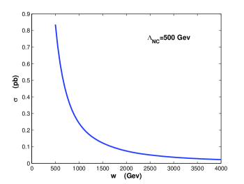
Figure 3: The relation between $\sigma$ and $w$ for $e^{+}e^{-}\rightarrow\mu^{+}\mu^{-}\gamma$

The NC correction for the cross-section varies with $w$ is shown in Fig. 4, where $\Lambda_{NC}=500\,{\mathrm{GeV}}$.

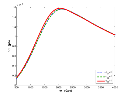
Figure 4: The relation between ${(\Delta\sigma)}_{NC}$ and $w$ for $e^{+}e^{-}\rightarrow\mu^{+}\mu^{-}\gamma$

From Fig. 4, it is found that the differences among the curves for $c_{01}=1$, $c_{02}=1$ and $c_{03}=1$ are small. In fact, the curves of ${(\Delta\sigma)}_{NC}$ with $c_{01}=1$ and $c_{02}=1$ are almost identical. We will only discuss the case with $c_{03}=1$ in the following analysis if there is no indication.

${(\Delta\sigma)}_{NC}$ does not increase monotonously with $w$, but there exists a kurtosis distribution. For $\Lambda_{NC}=500\,{\mathrm{GeV}}$, a maximum appears when the energy of collision particles $w=2258\,{\mathrm{GeV}}$. It implies that there is an optimal collision energy to observe NC effect in this process. However, we do not know the exact value of NC scale energy $\Lambda_{NC}$. We have to determine it at first. To do this, it is useful to establish the relation between NC scale energy and optimal collision energy $w_{o}$, which is shown as in Fig.5.

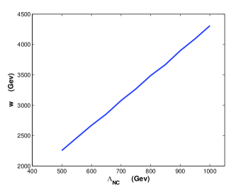
Figure 5: The optimal collision energy $w_{o}$ vs NC scale energy $\Lambda_{NC}$ for $e^{+}e^{-}\rightarrow\mu^{+}\mu^{-}\gamma$

Numerically, we get

$$w_{o}=229.263+4.067\Lambda_{NC}\;\;\;\;(\,{\mathrm{GeV}}).$$ (25)

Roughly, the optimal collision energy is about four times of NC scale energy. In principle, the NC effects could be detected when the particle energy is higher than $\Lambda_{NC}$, and the NC scale energy $\Lambda_{NC}$ is nothing but the characteristic energy at which the difference between QFT and NC QFT emerges. However, it is very difficult to determine directly such a characteristic energy, because the difference increases gradually, so that we do not know where is the start point of the difference. Determination of an optimal collision energy at which NC correction of scattering cross section arrives at the maximum is much easier, because determination of a highest point of curve is much easier than determination of an inflexion of curves in mathematics. If the optimal collision energy $w_{o}$ for NC effect is determined in the next generation colliding experiment by increasing gradually the energy of collision particles, then the NC QED scale energy $\Lambda_{NC}$ can be determined by relation eq.(25). This is an indirect but effective way. It is interesting to note that this linear relation also arise in Möller scattering and Bhabha scattering sheng .

Because this process is higher order in $\alpha$ ( ${\cal O}(\alpha^{3})$ ) comparing with other $e^{+}e^{-}\rightarrow l^{+}l^{-}$ processes, its value of ${(\Delta\sigma)}_{NC}$ is less than one percent of others. The higher precision tests, thus, has to be necessary, which means the luminosity of electron-positron beam should be increased (e.g. $10^{35}cm^{-2}s^{-1}$) so that this effect can be determined. In order to increase the percentage of NC correction to the cross section, another method is to use directly the anisotropic property of space-time, which is inherent characteristic of noncommutative geometry. This anisotropy will be eliminated partly after the integration respect to both polar angle and azimuthal angle for total scattering cross section. Measuring the difference of the differential cross sections at different polar angles not only can keep this inherent anisotropy, but also can reduce the systematic error of measurements.

When collision energy $w=2258Gev$ and $\Lambda_{NC}=500Gev$, the differential cross-section for commuting QED(right) and their NC correction(left) varying with $\cos\gamma$ are shown as in Fig.6. The difference of the differential cross section for QED and its NC correction between $\gamma=\pi/4$ and $\gamma=\pi/2$ is 0.0042pb and 0.0015pb respectively. Their ratio is $35.7\%$, which is much larger than the ratio between total cross section and its NC correction. It should be noted that the observation angles $\gamma$ should be not less than $\pi/4$ in order to obtain a larger ratio, because the differential cross section for commuting QED has a remarkably nonlinear increase with $\cos\gamma$ in contrast to slowly increase for its NC correction when $\cos\gamma>0.7$ or $\gamma<\pi/4$. The NC correction of the differential cross section is also small although this ratio is large, so the NC effects can be detected only when the luminosity of electron-positron beam is large enough.

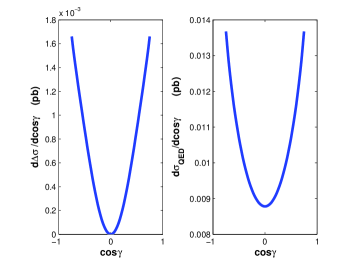
Figure 6: The differential cross-section and its NC correction vs $\cos\gamma$

V CONCLUSION AND DISCUSSION

The noncommutative corrections to the cross section for process $e^{+}e^{-}\rightarrow\mu^{+}\mu^{-}\gamma$ is studied and three new results are obtained. First, the higher collision energy in $e^{+}e^{-}\rightarrow\mu^{+}\mu^{-}\gamma$ does not always provide a better avenue to explore noncommutative effect. But there is an optimal collision energy to get the greatest noncommutative correction to total scattering section. In order to explore the noncommutative effects in the next generation international linear collider, we shall choose the optimal collision energy as the running energy with enough luminosity of electron-positron beam. This conclusion is reasonable, because the noncommutative effects do not more readily appear at low collision energy ( the collision energy must be higher than the NC scale energy $\Lambda_{NC}$ ), and the NC correction will decrease due to the total scattering section decrease with collision energy increase.

Second, there is a linear relation between the optimal collision energy and the NC QED scale energy $\Lambda_{NC}$ given by eq.(25). If the optimal collision energy is determined by increasing gradually the energy of collision particles from hundreds of $\,{\mathrm{GeV}}$ to several $\,{\mathrm{TeV}}$ in the next generation linear collider, then the NC QED scale energy can be determined from the given linear relation in an indirect but effective way.

Third, there is an experimental method to improve the precision of determining NC effects by measuring the difference of the differential cross sections at different polar angle; which not only can keep the inherent anisotropy, but also can reduce the system error of measurements. It is significant to explore NC effects for the process $e^{+}e^{-}\rightarrow\mu^{+}\mu^{-}\gamma$, because this process is one of the higher precision experiments to test ordinary QED.

In presenting these results, the Z-boson exchange contribution has not been included. If Z-boson and photon have the same vertex structure assumed as in Ref.Hewett01 , we can argue that the linear relation between optimal collision energy and NC QED scale energy$\Lambda_{NC}$ will hold, and we only need to modify the proportionality constant to account for the Z-boson exchange contribution.

It is interesting to note that, because of the anisotropy of space-time, the NC effects will be different at different site and different time for the same experiment. The dependence of NC corrections to differential cross section on longitude and latitude of experiment site and time is much stronger than that for total cross section. It is possible to determine the NC effects by observing the change of differential cross section with time, but we have to choose proper experiment site.

Acknowledgments:

The authors would like to thank referee’s comments and suggestions, and M.X. Luo and H.B. Yu for their useful discussions, also thank the hospitality and support for the Abdus Salam International Centre for Theoretical Physics, Trieste, Italy, where this work is completed mainly. This work is also supported in part by the funds from NSFC under Grant No.90303003.

References

- (1) H. S. Snyder, Phys. Rev. D 71, 38(1947).
- (2) A. Connes, M. R. Douglas and A. Schwarz, J.High Energy Phys. 02, (1998) 003.
- (3) M. R. Douglas and C. Hull, J.High Energy Phys. 02, (1998) 008.
- (4) N. Seiberg and E. Witten, J.High Energy Phys. 09, (1999) 032.
- (5) I. F. Riad and M. M. Sheikh-Jabbari, J.High Energy Phys.08,(2000) 045; M. M. Sheikh-Jabbari,Phys.Rev.Lett. 84, 5265(2000).
- (6) C. P. Martin and D. Sanchez-Ruiz,Phys.Rev.Lett. 83, 476(1999).
- (7) N. Ishibashi, S.Iso, H. Kawai and Y. Kitazawa, Nucl.Phys. B573, 573(2000).
- (8) I. Y. Aref’eva, D. M. Belov and A. S. Koshelev, Phys.Lett. B476, 431(2000).
- (9) F. J.Petriello, Nucl.Phys. B601, 169(2001).
- (10) S. M. Carroll, J. A. Harvey, V. A. Kostelecky, C. D. Lane, and T. Okamoto, Phys. Rev. Lett.87, 141601(2001).
- (11) N.Seiberg, L. Susskind and N.Toumbas, J.High Energy Phys. 06,(2000) 044.
- (12) A. Anisimov, T. Banks, M. Dine, M. Graesser, Phys. Rev. D 65, 085032(2002).
- (13) M. Chaichian, P. Presnajder, A. Tureanu, Phys. Rev. Lett. 94, 151602 (2005).
- (14) N. Arkani-Hamed, S. Dimopoulos and G. Dvali,Phys. Rev. D59, 086004(1999) ; E. Witten, Nucl. Phys. B471, 135(1996); P. Horava and E. Witten, Nucl. Phys. B460, 506(1996).
- (15) J.L. Hewett, F. J. Petriello and T. G. Rizzo, Phys.Rev. D64, 075012(2001); T. G. Rizzo, Int.J.Mod.Phys. A18, 2797(2003).
- (16) J. Kamoshita,hep-ph/0206223
- (17) H. Arfaei and M. H. Yavartanoo, hep-th/0010244.
- (18) S. Baek, D.K.Ghosh, X.G.He and W.-Y. P. Hwang, Phys.Rev. D64, 056001 (2001).
- (19) S. Godfrey, M.A. Doncheski,Phys.Rev. D65, 015005 (2002).
- (20) OPAL Collaboration,G. Abbiendi et al., Phys.Lett. B568, 181 (2003).
- (21) Z.M.Sheng,Y.M.Fu and H.Yu, Chin.Phys.Lett. 22, 561(2005).
- (22) A. Devoto,S.Di Chiara,and W.W.Repko,Phys. Rev.D 72 056006 (2005).
- (23) U. Mosco, Il Nuovo Cimento, 33, 3395 (1964); G. Longhi, Il Nuovo Cimento, 35, 1122 (1965).
- (24) F.J. Petriello, Phys. Rev. D 67, 033006 (2003).
- (25) M. Chaichian, M. M. Sheikh-Jabbari, A. Tureanu, Phys. Rev. Lett. 86, 2716 (2001).