Stability of multidimensional black holes: complete numerical analysis

Abstract

We analyze evolution of gravitational perturbations of $D$-dimensional Schwarzschild, Reissner-Nordström, and Reissner-Nordström-de Sitter black holes. It is known that the effective potential for the scalar type of gravitational perturbations has negative gap near the event horizon. This gap, for some values of the parameters $Q$ (charge), $\Lambda$ (cosmological constant) and $D$ (number of space-time dimensions), cannot be removed by S-deformations. Thereby, there is no proof of (in)stability for those cases. In the present paper, by an extensive search of quasinormal modes, both in time and frequency domains, we shall show that spherically symmetric static black holes with arbitrary charge and positive (de Sitter) lambda-term are stable for $D=5,6,\ldots 11$. In addition, we give a complete numerical data for all three types (scalar, vector and tensor) of gravitational perturbations for multi-dimensional black holes with charge and $\Lambda$-term. The influence of charge, $\Lambda$-term and number of extra dimensions on black hole quasinormal spectrum is discussed.

I Introduction

With the development of the string theory and higher-dimensional brane-world models, black holes in more than four space-time dimensions became a key subject in the modern high energy physics. Nevertheless, one of the first $D$-dimensional generalizations of the Schwarzschild metric was done, yet, in 1963 by Tangherlini Tangherlini:1963bw . This solution has attracted considerable interest recent years, in the context of brane-world models brane-world , and, for asymptotically anti-de Sitter case, within AdS/CFT correspondence AdSCFT . Different generalizations of the Tangherlini metric were found generalD . and their properties were investigated in propertyD . One of the most important property of a black hole metric is stability. Space-times unstable against small metric perturbations should not exist, or need some other, probably quantum, mechanisms to provide stability. If a black hole is unstable, small perturbations must grow with time, being governed by characteristic complex frequencies $\omega$, called quasinormal modes. These frequencies form a spectrum of the response of a black hole to the external perturbation. Contribution of all modes can be seen in the time domain Price-Pullin . Until now, during recent few years, evolution of perturbations of the $D$-dimensional black holes was investigated in a number of works. A lot of papers were devoted to perturbations of scalar test fields propagating in the vicinity of spherically symmetric black holes scalarD . Scalar QNMs of higher-dimensional Kerr black holes were analyzed in scalarD-Kerr . Quasinormal spectrum of Standard Model fields for brane-localized black holes were investigated in Berti:2003yr ; Abdalla:2006qj ; Kanti:2005xa ; Kanti:2006ua . In Kanti:2005xa , a variety of brane-localized backgrounds (Schwarzschild, Reissner-Nordström and Schwarzschild-(anti) de Sitter) were investigated, and it was shown that an increase in the number of hidden, extra dimensions results in the faster damping of all fields living on the brane. In Kanti:2006ua rotating black holes on the brane were considered, and, it was shown that the brane-localized field perturbations are longer-lived when the higher-dimensional black hole rotates faster.

In the context of Tev-gravity scenarios, the gravitational energy loss in high energy particles collisions was considered in Berti:2003si , where was found energy spectra, total energy and angular distribution of the emitted gravitational radiation. The further steps were analysis of the graviton emission form the higher dimensional black holes Cornell:2005ux and the close limit analysis for head-on collision of two black holes in higher dimensions Yoshino:2005ps ; Yoshino:2006kc .

In addition, some analytical solutions were found in different $D>4$ space-times D-exact . The high overtone asymptotics for perturbations of $D$-dimensional black holes were considered in highND .

After appearing of the paper of Kodama and Ishibashi Kodama:2003kk ; Kodama:2003jz ; Ishibashi:2003ap , where gravitational perturbations of the $D$-dimensional spherically symmetric black hole with charge and $\lambda$-term were reduced to the Schrodinger wave-like equations:

$$\frac{d^{2}\Psi_{i}}{dr_{*}^{2}}+(\omega^{2}-V_{i}(r))\Psi_{i}=0,$$ (1)

the low-laying gravitational quasinormal modes were found found in Konoplya:2003dd with the help of the WKB method WKB . In (1), $i$ runs $T$, $V$, $S$, because for $D>4$, in addition to the well-known in four dimensions axial and polar perturbations, which are vector and scalar types of gravitational perturbations respectively, there appears a new type of gravitational perturbations called tensor one. For $D$-dimensional Reissner-Nordström-(anti)-de Sitter black holes the tensor type of gravitational perturbations coincide with perturbations of test scalar filed. In the Einstein theory with the Gauss-Bonnet term, from works Dotti:2005sq ; Konoplya:2005sy ; Gleiser:2005ra , it follows that this coincidence does not take place.

An important feature of the gravitational perturbations is that the effective potentials which governs the scalar type of the perturbations has negative gap for $D>7$, and this gap becomes deeper when $D$ is increased. If the effective potential $V_{i}(r)$ is positive definite everywhere outside the black hole, event horizon, the differential operator

$$\frac{d^{2}}{dr_{*}^{2}}+\omega^{2}$$

is positive self-adjoint operator in the Hilbert space of the square integrable functions of $r^{*}$. As a result, any solution of the wave equation with compact support is bounded, what implies stability. In some cases this negative gap of the potential can be removed by the so-called S-deformation of the potential which does not change the property of stability Ishibashi:2003ap . In this way Ishibashi and Kodama in Kodama:2003kk ; Kodama:2003jz ; Ishibashi:2003ap , showed that $D$-dimensional Schwarzschild black holes are stable against all three types of gravitational perturbations. Yet, the potential for scalar type of gravitational perturbations of Reissner-Nordström black holes cannot be made positive definite by S-deformation, and therefore the question of stability of charged multidimensional black holes left open. That is why to judge about (in)stability of black holes we have to consider evolution of gravitational perturbations of $D$-dimensional black hole with special emphasis in scalar type of gravitational perturbations.

Note, that with the help of the WKB method, one can find only low laying modes for not very large $D$ Konoplya:2003dd . Therefore we have to apply here the Frobenius method Leaver:1985ax . Yet, even Frobenius method shows rather bad convergence for higher $D$ and, this made us to apply, alternatively, the time-domain approach. In the present paper we have found all three types of gravitational quasinormal modes and have shown that the D=5-11 Reissner-Nordström(-de Sitter) black holes are stable for any values of charge or $\Lambda$-term.

The paper is organized as follows. In Sec. II we give the basic formulas and discuss the range of parameters for the $D$-dimensional Reissner-Nordström(-de Sitter) metric and of its gravitational perturbations. Sec III describes the numerical method we used in time and frequency domain. Sec III relates the obtained quasinormal modes and time-domain profiles for Reissner-Nordström(-de Sitter) black holes in $D=5,6,\ldots 11$ space-time dimensions. Finally we discuss the obtained results and conclude that all considered cases are stable.

II Basic formulas

The metric of the $D$-dimensional Reissner-Nordström-de-Sitter black holes is given by the formula

$$ds^{2}=f(r)dt^{2}-\frac{dr^{2}}{f(r)}-r^{2}(d\theta^{2}+sin^{2}\theta d\phi^{2}).$$ (2)

where

$$f(r)=1-X+Z-Y,$$ (3)

$$X=\frac{2M}{r^{d-1}},\qquad Y=\frac{2\Lambda r^{2}}{d(d+1)},\qquad Z=\frac{Q^{2}}{r^{2d-2}},$$

The wave equation can be re-written in the form

$$\left(\frac{\partial^{2}}{\partial t^{2}}-\frac{\partial^{2}}{\partial r_{*}^{2}}\right)\Psi(t,r)=-V(r)\Psi(t,r),$$ (4)

where the tortoise coordinate $r_{*}$ is defined as

$$dr_{*}=\frac{dr}{f(r)}.$$ (5)

The effective potentials for tensor

$$V_{T}(r)=\frac{f(r)}{r^{2}}\left(\lambda+d+\frac{f^{\prime}(r)rd}{2}+\frac{f(r)d(d-2)}{4}\right)$$ (6)

and vector gravitational perturbations

$$V_{V}(r)=\frac{f(r)}{r^{2}}\left(\lambda+d\pm\sqrt{X^{2}\frac{(d^{2}-1)^{2}}{4}+2Z\lambda d(d-1)}\right.$$

$$+\left.\frac{d(d-2)(1-Y)+Zd(5d-2)-X(d^{2}+2)}{4}\right)$$ (7)

are designated as $V_{T}$, $V_{V}$ respectively.

The effective potential for the scalar type is given by

$$V_{S}(r)=f(r)\frac{U(r)}{16r^{2}H(r)^{2}},$$ (8)

where

$$H(r)=\lambda+X\frac{d(d+1)}{2}-Zd^{2},$$ (9)

$$U(r) = \left(-d^{3}(d+1)^{2}(d+2)X^{2}+4d^{2}(d+1)\left(d(d^{2}+6d-4)Z+3(d-2)\lambda\right)X-12d^{5}(3d-2)Z^{2}-\right.$$

$$\left.-8d^{2}(11d^{2}-26d+12)\lambda Z-4(d-2)(d-4)\lambda^{2}\right)Y+d^{4}(d+1)^{2}X^{3}+d(d+1)\left(-3d^{2}(5d^{2}-5d+2)Z+\right.$$

$$\left.+4(2d^{2}-3d+4)\lambda+d(d-2)(d-4)(d+1)\right)X^{2}+4d\left(d^{2}(4d^{3}+5d^{2}-10d+4)Z^{2}-\right.$$

$$\left.-\left(d(34-43d+21d^{2})\lambda+d^{2}(d+1)(d^{2}-10d+12)\right)Z-3(d-4)\lambda^{2}-3d(d+1)(d-2)\lambda\right)X-$$

$$-4d^{5}(3d-2)Z^{3}+4)\lambda+12d^{2}\left(2(-6d+3d^{2}+4)\lambda+d^{2}(3d-4)(d-2)\right)Z^{2}+4(13d-4)(d-2)\lambda^{2}Z+$$

$$+8d^{2}(11d^{2}-18d+4)\lambda Z+16\lambda^{3}+4d(d+2)\lambda^{2},$$

Here we used $d=D-2$, $\lambda=(l+d)(l-1)$ and $l$ is the multipole number.

We shall measure all the quantities in the units of the horizon radius. Thus we define

$$2M=1+Q^{2}-2\Lambda/d(d+1).$$ (10)

In order to parameterize the cosmological constant, we introduce the parameter $\rho=1/r_{c}<1$, where $r_{c}$ is the cosmological horizon. The value $\rho=0$ corresponds to the pure $D$-dimensional Reissner-Nordström black hole. Then, $\Lambda$ in terms of $Q$ and $\rho$ can be find from the equation

$$f(r_{c})=f(1/\rho)=0.$$ (11)

Solving the equation (11), one can find

$$\Lambda=\frac{d(d+1)}{2}\frac{1-\rho^{1-d}+Q^{2}(1-\rho^{d-1})}{1-\rho^{-d-1}}.$$ (12)

It is clear that for each $\Lambda$ there is some extremal charge $Q_{ext}$. The value of $Q_{ext}$ can be found from

$$f^{\prime}(1)=0.$$ (13)

For any charge $Q>Q_{ext}$, the definition (10) is not correct because in this case, the real event horizon has radius greater than one.

Substituting (12) into (13), one can find

$$Q_{ext}^{2}=\frac{(d-1)(1-\rho^{d+1})-\rho^{2}(d+1)(1-\rho^{d-1})}{(d-1)(1-\rho^{d+1})-\rho^{d+1}(d+1)(1-\rho^{d-1})}.$$ (14)

Within this paper we shall use $\rho$ and $q=Q/Q_{ext}$ as the black hole parameters. Note that the formulas (14) and (12) allow us to find $Q$ and $\Lambda$ in terms of $0\leq\rho<1$ and $0\leq q<1$. In the particular asymptotically flat case ($\Lambda=0$), we have $Q_{ext}=1$ and, therefore, $Q=q$.

III Numerical methods for frequency and time domains

III.1 Frequency domain

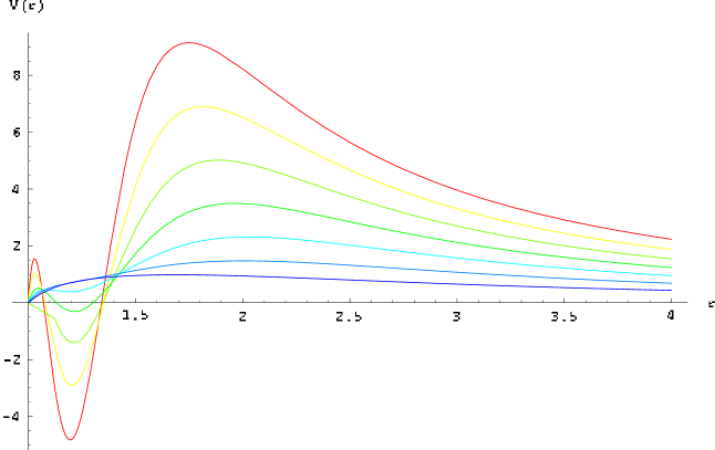
Figure 1: Effective potentials for gravitational perturbations of scalar type, $D=5$ (blue)…$D=11$ (red) ($l=2$, $Q=0$, $\Lambda=0$). For higher $D$ both the peak and the negative gap of the potential increase.

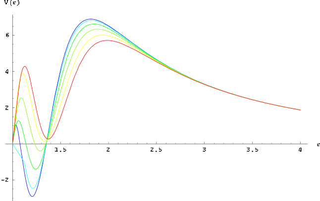
Figure 2: Effective potentials for gravitational perturbations of scalar type, $Q=0$ (blue), $Q=0.2$ (light blue), $Q=0.4$ (green), $Q=0.6$ (light green), $Q=0.8$ (yellow), $Q=0.98$ (red) ($l=2$, $D=10$, $\Lambda=0$). Increasing of the charge $Q$ cause the negative gap to move upwards. For some $Q$ the minimum of the potential becomes positive.

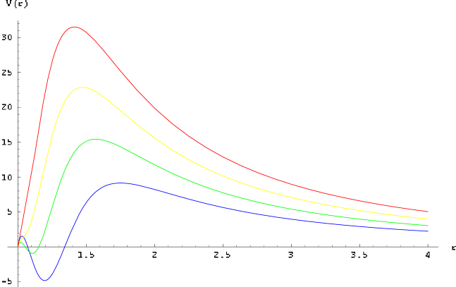
Figure 3: Effective potentials for gravitational perturbations of scalar type, $l=2,3,4,5$ (blue, green, yellow, red) ($D=11$, $Q=0$, $\Lambda=0$). For high multipole numbers the potential minimum disappears. Thus for $8\leq D\leq 10$ the negative gap exists only for the lowest multipole number $l=2$.

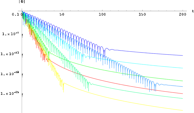
Figure 4: Time-domain profiles for gravitational perturbations of scalar type ($Q=0$, $\Lambda=0$) for $D=5$ (blue)…$D=11$ (red) at the same point $r=2$. Profile for higher $D$ decays quicker.

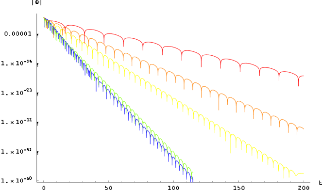
Figure 5: Time-domain profiles for gravitational perturbations of scalar type ($Q=0$, $D=11$) for $\rho=0.3$ (blue), $\rho=0.5$ (green), $\rho=0.7$ (yellow), $\rho=0.8$ (orange), $\rho=0.9$ (red). Profile for higher $\rho$ decays slower.

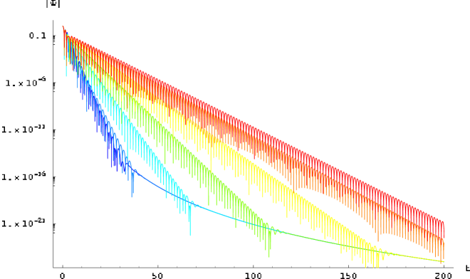
Figure 6: Time-domain profiles for gravitational perturbations of scalar type ($\Lambda=0$, $D=11$) for $Q=0$ (dark blue), $Q=0.5$ (blue), $Q=0.6$ (light blue), $Q=0.7$ (green), $Q=0.8$ (yellow), $Q=0.9$ (orange), $Q=0.98$ (red). Profile for higher $Q$ decays slower.

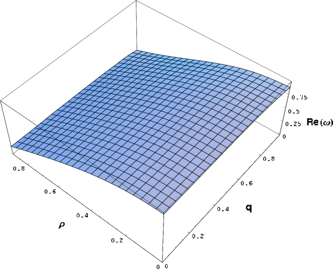
Figure 7: Real and imaginary part of the fundamental quasinormal frequency of gravitational perturbations of scalar type as a function of $q$ and $\rho$ ($D=5$, $l=2$).

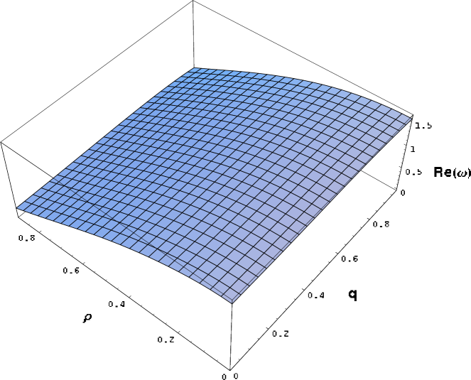
Figure 8: Real and imaginary part of the fundamental quasinormal frequency of gravitational perturbations of scalar type as a function of $q$ and $\rho$ ($D=8$, $l=2$).

Figure 9: Real and imaginary part of the fundamental quasinormal frequency of gravitational perturbations of scalar type as a function of $l$ ($D=9$, $q=0.5$, $\rho=0.3$). The solid line represents high multipole WKB formula.

By definition, the quasi-normal modes are eigenvalues of $\omega$ with the boundary conditions which correspond to the outgoing wave at the cosmological horizon (or spatial infinity when $\rho=0$) and the ingoing wave at the black hole horizon.

In order to find quasi-normal spectrum for the considered types of perturbations, we shall use the continued fraction method Leaver:1985ax . The equation (1) has a different kind of singularity at $r=1/\rho$: if $\rho=0$, the singularity is irregular at infinity as usually for the Schwarzschild case

$$\Psi(r\rightarrow\infty)\propto e^{i\omega r},$$

while for $\rho>0$ the point of the cosmological horizon is a regular singularity Yoshida:2003zz

$$\Psi\left(r\rightarrow\frac{1}{\rho}\right)\propto\left(\rho-\frac{1}{r}\right)^{i\omega/f^{\prime}\left(\frac{1}{\rho}\right)}.$$

It turns out, that we can simply exclude this singularity by the introducing of the new function

$$\Phi=e^{-i\omega r^{*}}\Psi,$$

where $\Phi$ satisfies

$$\frac{d^{2}\Phi}{dr^{*2}}+2i\omega\frac{d\Phi}{dr^{*}}-V\Phi=0.$$ (15)

In order to satisfy the QNM boundary conditions, the function $\Phi$ has to be convergent at $r=1/\rho$. Thus, the only valuable singularity remains at $r=1$. Taking into account that there is only the ingoing wave at the event horizon, one can find

$$\Phi(r\rightarrow 1)\propto(r-1)^{-2i\omega/f^{\prime}(1)}.$$

Finally, we obtain

$$\Phi(r)=\left(1-\frac{1}{r}\right)^{\frac{-2i\omega}{f^{\prime}(1)}}y(r),$$ (16)

where y(r) is convergent on $r\in[1,1/\rho]$. The appropriate Frobenius series for $y(r)$ are

$$y(r)=\sum_{i=0}^{\infty}a_{n}\left(\frac{r-1}{r-R}\frac{1-R\rho}{1-\rho}\right)^{n},$$ (17)

where $R<1$ is an arbitrary parameter.

The expansion (17) is valid if all singular points (except those on the event and the cosmological horizons) satisfy inequality

$$\left|\frac{r-1}{r-R}\frac{1-R\rho}{1-\rho}\right|>1.$$ (18)

Since for the effective potential of the gravitational perturbations of vector and tensor types the singular points are 1) $r=0$ and 2) the solutions of the equation $f(r)=0$, we can always find such $0\leq R<1$ to satisfy inequality (18) for all the additional singular points. The latter follows from the definition of the horizons, which are the two larger positive solutions of the equation $f(r)=0$.

After $R$ is fixed, following Zhidenko:2006rs , one can find the recurrence relation for the coefficients $a_{n}$ in (17) and use the continued fraction method with the generalized Nollert improvement Nollert . It turns out, that the convergence of the method becomes worse when $R\rightarrow 1$. Thus one has to choose the minimal value of $R$ that satisfies the inequality (18) for all singular points, except those at the event and the cosmological horizons. For $D\leq 9$ this point is $R=r_{-}$, which is the remaining positive root of $f(r)$ (or $R=0$ if $f(r)$ has no more positive root), and the continued fraction method converges without the generalized Nollert improvement. For larger $D$ such $R$ is, generally, not a singular point of the equation (15) and the convergence of the method is provided by the procedure Zhidenko:2006rs . Alternatively, for $D>9$ one can continue the Frobenius series through some midpoints. This method was used in Rostworowski:2006bp and our results are completely in agreement with it.

For the scalar-type gravitational perturbations, the equation (15) has additional singularities, which are the roots of $H(r)$. Thus, in higher dimensions $D\geq 7$, for some values of $\rho$, $q$ and $l$ there is no such $R<1$, which satisfies the inequality (18) for all the singular points. Therefore, for those cases one should use only the technique developed in Rostworowski:2006bp . Practically, the continued fraction coefficients appear to be so complicated, that we are unable to compute QNMs with this method during reasonable time, even for low dimensions, except the case when $\rho=0$.

III.2 Time domain

Alternatively, we shall use the time-domain analysis based on the standard integration scheme for the wave-like equations (4), which is described for instance in Price-Pullin . This approach has no limitations of the parameters for the scalar-type perturbations. Moreover, it appears to be quicker for the perturbations of scalar type, when $D$ is large or $\rho\neq 0$. Since we can see the real signal which contains all the frequencies, this method also provides the most direct evidence of the black hole stability. It allows also to find out asymptotical tails.

In detail, we applied a numerical characteristic integration scheme,that uses the light-cone variables $u=t-r_{\star}$ and $v=t+r_{\star}$. In the characteristic initial value problem, initial data are specified on the two null surfaces $u=u_{0}$ and $v=v_{0}$. The discretization scheme we used, is

$$\Psi(N)=\Psi(W)+\Psi(E)-\Psi(S)$$ (19)

$$\mbox{}-\Delta^{2}\frac{V(W)\Psi(W)+V(E)\Psi(E)}{8}+\mathcal{O}(\Delta^{4})\ ,$$

where we have used the following definitions for the points: $N=(u+\Delta,v+\Delta)$, $W=(u+\Delta,v)$, $E=(u,v+\Delta)$ and $S=(u,v)$.

IV Evolution of gravitational perturbations

IV.1 Scalar type of gravitational perturbations

Table 1: Fundamental modes ($l=2$, $\Lambda=0$) of gravitational perturbations of scalar type calculated by the continued fraction method (the first value) and by the time-domain simulation (the second value). For higher $D$ the behavior of the time-domain profile is very irregular. Thus QNMs finding with high accuracy is more complicated.

$Q$	$D=5$	$D=6$	$D=7$	$D=8$	$D=9$	$D=10$
$0$	$0.94774-0.25609i$	$1.13690-0.30358i$	$1.33916-0.40086i$	$\!\!-$	$\!\!-$	$\!\!-$
	$0.94773-0.25609i$	$1.13690-0.30357i$	$1.33917-0.40084i$	$1.56390-0.60312i$	$1.99898-0.86335i$	$2.45~{}-~{}0.98i$
$0.1$	$0.94842-0.25523i$	$1.13830-0.30117i$	$1.34131-0.39489i$	$\!\!-$	$\!\!-$	$\!\!-$
	$0.94841-0.25522i$	$1.13830-0.30117i$	$1.34132-0.39488i$	$1.56327-0.58781i$	$1.98516-0.85771i$	$2.45~{}-~{}0.97i$
$0.2$	$0.95032-0.25263i$	$1.14225-0.29422i$	$1.34745-0.37794i$	$\!\!-$	$\!\!-$	$\!\!-$
	$0.95032-0.25262i$	$1.14225-0.29422i$	$1.34745-0.37793i$	$1.56447-0.54593i$	$1.93834-0.83840i$	$2.41~{}-~{}0.97i$
$0.3$	$0.95304-0.24830i$	$1.14802-0.28342i$	$1.35661-0.35246i$	$\!\!-$	$\!\!-$	$\!\!-$
	$0.95303-0.24829i$	$1.14802-0.28342i$	$1.35661-0.35246i$	$1.57120-0.48765i$	$1.83938-0.76949i$	$2.34~{}-~{}0.96i$
$0.4$	$0.95585-0.24218i$	$1.15446-0.26977i$	$1.36721-0.32163i$	$\!\!-$	$\!\!-$	$\!\!-$
	$0.95583-0.24217i$	$1.15447-0.26976i$	$1.36721-0.32163i$	$1.58264-0.42318i$	$1.79707-0.60660i$	$2.14~{}-~{}0.94i$
$0.5$	$0.95762-0.23407i$	$1.16006-0.25436i$	$1.37715-0.28865i$	$\!\!-$	$\!\!-$	$\!\!-$
	$0.95760-0.23405i$	$1.16006-0.25435i$	$1.37715-0.28865i$	$1.59530-0.35950i$	$1.80551-0.47879i$	$1.985-0.674i$
$0.6$	$0.95666-0.22363i$	$1.16290-0.23816i$	$1.38398-0.25627i$	$\!\!-$	$\!\!-$	$\!\!-$
	$0.95662-0.22361i$	$1.16289-0.23816i$	$1.38398-0.25627i$	$1.60536-0.30104i$	$1.81782-0.37688i$	$2.011-0.486i$
$0.7$	$0.95033-0.21055i$	$1.16059-0.22197i$	$1.38498-0.22676i$	$\!\!-$	$\!\!-$	$\!\!-$
	$0.95027-0.21052i$	$1.16060-0.22197i$	$1.38498-0.22675i$	$1.60921-0.25088i$	$1.82430-0.29638i$	$2.024-0.362i$
$0.8$	$0.93502-0.19538i$	$1.15025-0.20660i$	$\!\!-$	$\!\!-$	$\!\!-$	$\!\!-$
	$0.93490-0.19535i$	$1.15026-0.20659i$	$1.37723-0.20212i$	$1.60359-0.21163i$	$1.82052-0.23687i$	$2.023-0.275i$
$0.9$	$0.90758-0.18077i$	$1.12912-0.19364i$	$\!\!-$	$\!\!-$	$\!\!-$	$\!\!-$
	$0.90745-0.18075i$	$1.12913-0.19363i$	$1.35858-0.18465i$	$1.58656-0.18609i$	$1.80461-0.20010i$	$2.009-0.224i$
$0.98$	$0.87720-0.17177i$	$1.10420-0.18636i$	$\!\!-$	$\!\!-$	$\!\!-$	$\!\!-$
	$0.87707-0.17175i$	$1.10429-0.18641i$	$1.33609-0.17704i$	$1.56549-0.17657i$	$1.78451-0.18755i$	$1.990-0.208i$

Table 2: Fundamental modes ($l=2$, $Q=0$) of gravitational perturbations of scalar type calculated by the time-domain simulation. For higher $D$ the behavior of the time-domain profile is very irregular. Thus QNMs finding with high accuracy is more complicated.

$\rho$	$D=5$	$D=6$	$D=7$	$D=8$	$D=9$	$D=10$
$0$	$0.94774-0.25609i$	$1.13690-0.30358i$	$1.33916-0.40086i$	$1.56390-0.60312i$	$1.99898-0.86335i$	$2.45~{}-~{}0.98i$
$0.1$	$0.93336-0.25576i$	$1.12050-0.30461i$	$1.31868-0.39970i$	$1.53691-0.59412i$	$1.95602-0.86639i$	$2.41~{}-~{}0.99i$
$0.2$	$0.89204-0.25366i$	$1.07169-0.30664i$	$1.25828-0.39567i$	$1.45301-0.56754i$	$1.81939-0.87158i$	$2.28~{}-~{}1.00i$
$0.3$	$0.82569-0.24749i$	$0.99203-0.30681i$	$1.16108-0.38781i$	$1.33119-0.52832i$	$1.56112-0.84743i$	$2.04~{}-~{}1.01i$
$0.4$	$0.73774-0.23477i$	$0.88551-0.30073i$	$1.03263-0.37458i$	$1.17909-0.48504i$	$1.31893-0.67923i$	$1.70~{}-~{}1.01i$
$0.5$	$0.63289-0.21293i$	$0.75787-0.28372i$	$0.87872-0.35286i$	$0.99978-0.44032i$	$1.11688-0.56723i$	$1.209-0.801i$
$0.6$	$0.51662-0.18156i$	$0.61591-0.25212i$	$0.70774-0.31741i$	$0.79938-0.38928i$	$0.89080-0.47868i$	$0.978-0.601i$
$0.7$	$0.39236-0.14257i$	$0.46597-0.20493i$	$0.52888-0.26326i$	$0.58941-0.32283i$	$0.64959-0.38903i$	$0.710-0.468i$
$0.8$	$0.26341-0.09797i$	$0.31181-0.14428i$	$0.34978-0.18904i$	$0.38262-0.23377i$	$0.41294-0.28050i$	$0.442-0.332i$
$0.9$	$0.12993-0.04982i$	$0.15447-0.07427i$	$0.17045-0.09844i$	$0.18471-0.12283i$	$0.19478-0.14745i$	$0.203-0.173i$

It is essential for our computations that the effective potential for charged black holes have the negative gap which cannot be ”removed” by S-deformation Ishibashi:2003ap ; Kodama:2003kk ; Kodama:2003jz for $D\geq 8$. This gives us the cases for suspecting instability. The fundamental quasinormal modes for scalar type of gravitational perturbations computed with Frobenius and time-domain techniques are given in Tables 1, 2. For $D=5,6,7$ Reissner-Nordström black holes ($\Lambda=0$), the real parts of QNMs increase with charge until some maximum, then decrease. For $D\geq 8$ $Re\omega$, for small $Q$, decreases as a function of $Q$, then increases and reaches some maximum and then, again decreases for close to the extremal $Q$. The imaginary part of the frequencies as a function of charge $Q$ monotonically decreases for all $D$ (Table 1). Note that in table 1 the calculations of QNMs were done for $D=5,6,7$ with both time-domain and Frobenius approaches. Yet, for higher $D$, the Frobenius method needs considerable computer time for converging. The time-domain picture of the decay for black holes with high $D=10,11,\ldots$ are different from lower dimensional cases: if for $D=5,6,\ldots 9$ we see always regular picture of time-domain decay (Fig. 4), for $D=10,11$, and for small $Q$ and $\Lambda$ the ringing is more irregular (in fact, the amplitude is irregular, that probably means the superposition of a few dominating modes) and quickly changes into tail behavior (Fig.5, Fig. 6). The time domain picture becomes again regular at larger $Q$ and $\Lambda$ (Fig.5, Fig. 6).

The fundamental modes for Schwarzschild -de Sitter black holes ($Q=0$) are given in Table 2. The real oscillation frequency usually monotonically decreases as a function of $\Lambda$-term. Note that literature on QNMs of the scalar type of gravitational perturbations in $D>4$ is very poor Konoplya:2003dd ; cardosoJHEP . Our computations show perfect coincidence with Frobenius method data of cardosoJHEP and very good coincidence with the WKB results of Konoplya:2003dd for scalar type of gravitational perturbations. Alternative approach for finding gravitational quasinormal modes is to consider the head-on collisions for higher dimensional theories Yoshino:2005ps ; Yoshino:2006kc . The comparison with our accurate numerical values of QNMs gives very good agreement for not large $D$: Thus for $D=5$ and $6$, we have $\omega=0.94773-0.25609i$, $\omega=1.13690-0.30357i$ respectively, while paper Yoshino:2005ps give the values $\omega=0.947-0.256i$, $\omega=1.139-0.305i$, i.e. the error in Yoshino:2005ps is indeed very small and is less than $1$ percent. For $D=9,10,11$ the method in Yoshino:2005ps shows superposition of the two dominating modes, one of which is very close to that obtained here. For instance for $D=4$, they have $\omega=2.47-0.99i$, while we obtained with time-domain approach $\omega=2.45-0.98i$. This small difference between our results is quite natural because different approximations were used: we considered the regime of small perturbations and in Yoshino:2005ps a close limit approximation was used. Therefore we conclude that the close limit approximation with Brill-Lindquist initial data is indeed a very accurate approach.

When both parameters $Q$ and $\Lambda$ are not vanishing, the quasinormal frequencies are again damping. An example of behavior of real and imaginary of $\omega$ as a function of $q$ and $\rho$ (which parameterize all the values of $Q$ and $\Lambda$) is given in Fig 7 for $D=5$ case and Fig 8 for $D=8$ case.

At large multi-pole numbers $\ell$, the WKB approach WKB becomes very accurate and one can obtain usually an analytical formula for the QN frequencies. For our case of Reissner-Nordström-de Sitter black holes, a cumbersome form of the effective potential with a lot of parameters makes it impossible to find a short QNM formula, which could be easily interpreted for general values of $M$, $Q$, $\Lambda$, $D$. Yet, if we fix all the above parameters the WKB formula in the lowest order gives, for example for $D=9$, $Q=0.5Q_{ext}$, $\rho=0.3$ (see Fig 9):

$$\omega=0.60897(\ell+3)-1.42338(n+1/2)i,\quad\ell\rightarrow\infty$$ (20)

Here we can see that in a similar fashion with a four-dimensional case, the real oscillation frequency is proportional to $\ell$ and the damping rate is approaching some constant value. Therefore one should not expect any instability from the regime of high $\ell$. Indeed, higher $\ell$ just raise the potential barrier and serve as a stabilizing factor: perturbations with higher $\ell$ are more stable than perturbations with lower $\ell$.

Finally, summarizing the extensive search for quasinormal modes for scalar type of gravitational perturbations, we conclude that the response to the external perturbations of the Reissner-Nordström-de Sitter black holes are represented by damping oscillations and therefore for all values of charge and $\Lambda$-term in $D=5,6,\ldots 11$ space-time dimensions, the Reissner-Nordström-de Sitter black holes are stable.

IV.2 Vector and tensor types of gravitational perturbations

Table 3: Fundamental modes ($l=2$, $\Lambda=0$) of gravitational perturbations of vector($"+"$) type calculated by the time-domain simulation.

$Q$	$D=5$	$D=6$	$D=7$	$D=8$	$D=9$	$D=10$
$0$	$1.46854-0.35242i$	$1.97832-0.49641i$	$2.47008-0.62640i$	$2.95282-0.74529i$	$3.43062-0.85514i$	$3.90559-0.95743i$
$0.1$	$1.47080-0.35064i$	$1.98180-0.49437i$	$2.47403-0.62391i$	$2.95761-0.74270i$	$3.43587-0.85244i$	$3.91135-0.95445i$
$0.2$	$1.47742-0.34551i$	$1.99114-0.48814i$	$2.48556-0.61683i$	$2.97099-0.73491i$	$3.45092-0.84399i$	$3.92777-0.94560i$
$0.3$	$1.48547-0.33667i$	$2.00371-0.47750i$	$2.50181-0.60482i$	$2.99037-0.72177i$	$3.47300-0.82999i$	$3.95228-0.93076i$
$0.4$	$1.49155-0.32391i$	$2.01585-0.46226i$	$2.51897-0.58770i$	$3.01180-0.70309i$	$3.49819-0.81005i$	$3.98080-0.90983i$
$0.5$	$1.49210-0.30723i$	$2.02337-0.44241i$	$2.53244-0.56546i$	$3.03033-0.67894i$	$3.52125-0.78433i$	$4.00792-0.88286i$
$0.6$	$1.48353-0.28708i$	$2.02189-0.41860i$	$2.53713-0.53882i$	$3.04036-0.65008i$	$3.53610-0.75362i$	$4.02713-0.85065i$
$0.7$	$1.46249-0.26477i$	$2.00727-0.39257i$	$2.52816-0.50988i$	$3.03633-0.61882i$	$3.53655-0.72040i$	$4.03167-0.81580i$
$0.8$	$1.42669-0.24279i$	$1.97680-0.36751i$	$2.50236-0.48241i$	$3.01453-0.58938i$	$3.51835-0.68929i$	$4.01676-0.78326i$
$0.9$	$1.37633-0.22431i$	$1.93086-0.34705i$	$2.46010-0.46053i$	$2.97522-0.56631i$	$3.48165-0.66523i$	$3.98235-0.75837i$
$0.98$	$1.32775-0.21336i$	$1.88525-0.33525i$	$2.41682-0.44832i$	$2.93363-0.55377i$	$3.44148-0.65248i$	$3.94338-0.74548i$

Table 4: Fundamental modes ($l=2$, $\Lambda=0$) of gravitational perturbations of vector($"-"$) type calculated by the time-domain simulation.

$Q$	$D=5$	$D=6$	$D=7$	$D=8$	$D=9$	$D=10$
$0$	$1.13400-0.32752i$	$1.52467-0.47412i$	$1.93447-0.61230i$	$2.35885-0.73871i$	$2.79285-0.85412i$	$3.23345-0.96025i$
$0.1$	$1.12873-0.32542i$	$1.51974-0.47195i$	$1.93008-0.60995i$	$2.35455-0.73593i$	$2.78882-0.85126i$	$3.22923-0.95699i$
$0.2$	$1.11323-0.31965i$	$1.50551-0.46553i$	$1.91694-0.60268i$	$2.34200-0.72777i$	$2.77645-0.84240i$	$3.21691-0.94756i$
$0.3$	$1.08935-0.31042i$	$1.48324-0.45520i$	$1.89595-0.59098i$	$2.32163-0.71475i$	$2.75614-0.82835i$	$3.19652-0.93271i$
$0.4$	$1.05895-0.29829i$	$1.45430-0.44154i$	$1.86800-0.57559i$	$2.29396-0.69786i$	$2.72819-0.81033i$	$3.16820-0.91389i$
$0.5$	$1.02349-0.28402i$	$1.41985-0.42551i$	$1.83391-0.55781i$	$2.25963-0.67875i$	$2.69314-0.79031i$	$3.13248-0.89327i$
$0.6$	$0.98411-0.26862i$	$1.38094-0.40854i$	$1.79473-0.53951i$	$2.21974-0.65967i$	$2.65228-0.77079i$	$3.09083-0.87359i$
$0.7$	$0.94199-0.25339i$	$1.33903-0.39228i$	$1.75230-0.52260i$	$2.17659-0.64270i$	$2.60824-0.75390i$	$3.04653-0.85697i$
$0.8$	$0.89871-0.23937i$	$1.29619-0.37763i$	$1.70919-0.50774i$	$2.13312-0.62808i$	$2.56415-0.73951i$	$3.00213-0.84311i$
$0.9$	$0.85578-0.22668i$	$1.25410-0.36428i$	$1.66671-0.49423i$	$2.09047-0.61471i$	$2.52102-0.72627i$	$2.95869-0.83045i$
$0.98$	$0.82248-0.21747i$	$1.22123-0.35412i$	$1.63310-0.48428i$	$2.05718-0.60463i$	$2.48645-0.71566i$	$2.92469-0.82086i$

Table 5: Fundamental modes ($l=2$, $Q=0$) of gravitational perturbations of vector($"+"$) type calculated by the continued fraction method (the first value) and by the time-domain simulation (the second value).

$\rho$	$D=5$	$D=6$	$D=7$	$D=8$	$D=9$	$D=10$
$0$	$1.46854-0.35243i$	$1.97830-0.49642i$	$2.47006-0.62642i$	$2.95278-0.74532i$	$3.43056-0.85518i$	$3.90550-0.95749i$
	$1.46854-0.35242i$	$1.97832-0.49641i$	$2.47008-0.62640i$	$2.95282-0.74529i$	$3.43062-0.85514i$	$3.90559-0.95743i$
$0.1$	$1.44629-0.34752i$	$1.95277-0.49123i$	$2.44074-0.62113i$	$2.91936-0.74005i$	$3.39283-0.84998i$	$3.86332-0.95241i$
	$1.44629-0.34751i$	$1.95278-0.49122i$	$2.44076-0.62112i$	$2.91940-0.74002i$	$3.39289-0.84994i$	$3.86341-0.95235i$
$0.2$	$1.38107-0.33291i$	$1.87596-0.47514i$	$2.35219-0.60449i$	$2.81847-0.72326i$	$3.27906-0.83327i$	$3.73627-0.93591i$
	$1.38107-0.33291i$	$1.87597-0.47513i$	$2.35221-0.60447i$	$2.81850-0.72323i$	$3.27911-0.83323i$	$3.73635-0.93586i$
$0.3$	$1.27723-0.30908i$	$1.74877-0.44702i$	$2.20360-0.57433i$	$2.64868-0.69214i$	$3.08771-0.80175i$	$3.52289-0.90433i$
	$1.27724-0.30908i$	$1.74877-0.44701i$	$2.20361-0.57431i$	$2.64871-0.69212i$	$3.08776-0.80172i$	$3.52296-0.90429i$
$0.4$	$1.14122-0.27698i$	$1.57512-0.40612i$	$1.99630-0.52809i$	$2.40957-0.64273i$	$2.81743-0.75044i$	$3.22147-0.85188i$
	$1.14122-0.27698i$	$1.57513-0.40611i$	$1.99631-0.52808i$	$2.40959-0.64271i$	$2.81747-0.75042i$	$3.22152-0.85185i$
$0.5$	$0.98025-0.23821i$	$1.36231-0.35313i$	$1.73596-0.46457i$	$2.10458-0.57170i$	$2.46965-0.67413i$	$2.83196-0.77182i$
	$0.98025-0.23821i$	$1.36231-0.35313i$	$1.73597-0.46456i$	$2.10460-0.57169i$	$2.46967-0.67412i$	$2.83199-0.77179i$
$0.6$	$0.80110-0.19466i$	$1.11935-0.29056i$	$1.43247-0.38547i$	$1.74298-0.47889i$	$2.05196-0.57025i$	$2.35987-0.65912i$
	$0.80110-0.19466i$	$1.11935-0.29055i$	$1.43248-0.38547i$	$1.74299-0.47888i$	$2.05198-0.57024i$	$2.35989-0.65910i$
$0.7$	$0.60947-0.14800i$	$0.85494-0.22164i$	$1.09744-0.29526i$	$1.33861-0.36881i$	$1.57929-0.44211i$	$1.81992-0.51489i$
	$0.60946-0.14801i$	$0.85494-0.22164i$	$1.09744-0.29526i$	$1.33862-0.36881i$	$1.57930-0.44210i$	$1.81993-0.51488i$
$0.8$	$0.40990-0.09947i$	$0.57648-0.14915i$	$0.74150-0.19890i$	$0.90581-0.24880i$	$1.06987-0.29887i$	$1.23394-0.34909i$
	$0.40990-0.09947i$	$0.57648-0.14915i$	$0.74150-0.19890i$	$0.90581-0.24880i$	$1.06987-0.29887i$	$1.23395-0.34909i$
$0.9$	$0.20588-0.04994i$	$0.28997-0.07491i$	$0.37338-0.09989i$	$0.45650-0.12490i$	$0.53948-0.14995i$	$0.62239-0.17505i$
	$0.20588-0.04994i$	$0.28997-0.07491i$	$0.37338-0.09989i$	$0.45650-0.12490i$	$0.53948-0.14995i$	$0.62239-0.17505i$

Table 6: Fundamental modes ($l=2$, $Q=0$) of gravitational perturbations of vector($"-"$) type calculated by the continued fraction method (the first value) and by the time-domain simulation (the second value).

$\rho$	$D=5$	$D=6$	$D=7$	$D=8$	$D=9$	$D=10$
$0$	$1.13400-0.32752i$	$1.52466-0.47412i$	$1.93446-0.61231i$	$2.35883-0.73874i$	$2.79281-0.85415i$	$3.23339-0.96031i$
	$1.13400-0.32752i$	$1.52467-0.47412i$	$1.93447-0.61230i$	$2.35885-0.73871i$	$2.79285-0.85412i$	$3.23345-0.96025i$
$0.1$	$1.11435-0.32445i$	$1.49999-0.47120i$	$1.90445-0.60980i$	$2.32356-0.73670i$	$2.75235-0.85255i$	$3.18778-0.95907i$
	$1.11435-0.32445i$	$1.50000-0.47119i$	$1.90447-0.60979i$	$2.32358-0.73668i$	$2.75238-0.85252i$	$3.18784-0.95902i$
$0.2$	$1.05738-0.31448i$	$1.42675-0.46085i$	$1.81478-0.60035i$	$2.21794-0.72854i$	$2.63114-0.84561i$	$3.05117-0.95321i$
	$1.05738-0.31448i$	$1.42676-0.46084i$	$1.81479-0.60034i$	$2.21796-0.72852i$	$2.63117-0.84558i$	$3.05122-0.95316i$
$0.3$	$0.96883-0.29608i$	$1.30898-0.43923i$	$1.66798-0.57863i$	$2.04364-0.70827i$	$2.43048-0.82708i$	$2.82473-0.93628i$
	$0.96883-0.29608i$	$1.30898-0.43923i$	$1.66798-0.57862i$	$2.04365-0.70826i$	$2.43051-0.82706i$	$2.51248-0.89812i$
$0.4$	$0.85670-0.26872i$	$1.15581-0.40298i$	$1.47213-0.53811i$	$1.80689-0.66732i$	$2.15518-0.78734i$	$2.51245-0.89815i$
	$0.85671-0.26872i$	$1.15581-0.40297i$	$1.47213-0.53810i$	$1.80690-0.66731i$	$2.15520-0.78732i$	$2.12471-0.82648i$
$0.5$	$0.72870-0.23352i$	$0.97927-0.35226i$	$1.24192-0.47539i$	$1.52193-0.59819i$	$1.81754-0.71592i$	$2.12469-0.82650i$
	$0.72870-0.23352i$	$0.97927-0.35225i$	$1.24192-0.47539i$	$1.52194-0.59818i$	$1.81755-0.71591i$	$1.68348-0.71083i$
$0.6$	$0.59065-0.19237i$	$0.78984-0.29049i$	$0.99434-0.39341i$	$1.21066-0.49989i$	$1.44075-0.60671i$	$1.68347-0.71085i$
	$0.59065-0.19237i$	$0.78984-0.29049i$	$0.99434-0.39341i$	$1.21066-0.49988i$	$1.44075-0.60671i$	$2.82477-0.93624i$
$0.7$	$0.44658-0.14710i$	$0.59441-0.22174i$	$0.74231-0.29939i$	$0.89505-0.38063i$	$1.05542-0.46492i$	$1.22478-0.55081i$
	$0.44658-0.14710i$	$0.59441-0.22174i$	$0.74231-0.29938i$	$0.89505-0.38063i$	$1.05543-0.46492i$	$1.22479-0.55081i$
$0.8$	$0.29911-0.09923i$	$0.39673-0.14920i$	$0.49222-0.20025i$	$0.58809-0.25289i$	$0.68581-0.30743i$	$0.78648-0.36396i$
	$0.29911-0.09923i$	$0.39673-0.14920i$	$0.49222-0.20025i$	$0.58809-0.25289i$	$0.68581-0.30743i$	$0.78648-0.36396i$
$0.9$	$0.14990-0.04991i$	$0.19842-0.07491i$	$0.24523-0.10006i$	$0.29132-0.12542i$	$0.33718-0.15110i$	$0.38309-0.17716i$
	$0.14990-0.04991i$	$0.19842-0.07491i$	$0.24523-0.10006i$	$0.29132-0.12542i$	$0.33718-0.15110i$	$0.38309-0.17716i$

Table 7: Fundamental modes ($l=2$, $\Lambda=0$) of gravitational perturbations of tensor type calculated by the continued fraction method.

$Q$	$D=5$	$D=6$	$D=7$	$D=8$	$D=9$	$D=10$
$0$	$1.51057-0.35754i$	$2.01153-0.50194i$	$2.49678-0.63188i$	$2.97469-0.75056i$	$3.44882-0.86013i$	$3.92095-0.96212i$
$0.1$	$1.50687-0.35527i$	$2.00760-0.49926i$	$2.49270-0.62893i$	$2.97048-0.74743i$	$3.44451-0.85686i$	$3.91654-0.95876i$
$0.2$	$1.49575-0.34858i$	$1.99579-0.49136i$	$2.48041-0.62030i$	$2.95782-0.73829i$	$3.43153-0.84736i$	$3.90328-0.94898i$
$0.3$	$1.47711-0.33773i$	$1.97601-0.47872i$	$2.45985-0.60659i$	$2.93664-0.72389i$	$3.40980-0.83247i$	$3.88107-0.93374i$
$0.4$	$1.45084-0.32326i$	$1.94822-0.46216i$	$2.43101-0.58890i$	$2.90695-0.70552i$	$3.37938-0.81368i$	$3.85000-0.91466i$
$0.5$	$1.41684-0.30600i$	$1.91251-0.44296i$	$2.39413-0.56881i$	$2.86911-0.68503i$	$3.34072-0.79303i$	$3.81063-0.89397i$
$0.6$	$1.37526-0.28717i$	$1.86940-0.42278i$	$2.35002-0.54830i$	$2.82423-0.66461i$	$3.29520-0.77285i$	$3.76452-0.87411i$
$0.7$	$1.32676-0.26838i$	$1.82018-0.40345i$	$2.30048-0.52922i$	$2.77447-0.64603i$	$3.24525-0.75485i$	$3.71440-0.85670i$
$0.8$	$1.27290-0.25118i$	$1.76696-0.38619i$	$2.24787-0.51240i$	$2.72233-0.62977i$	$3.19345-0.73917i$	$3.66296-0.84114i$
$0.9$	$1.21589-0.23645i$	$1.71184-0.37127i$	$2.19317-0.49714i$	$2.66790-0.61582i$	$3.14034-0.72614i$	$3.59458-0.78869i$

Table 8: Fundamental modes ($l=2$, $Q=0$) of gravitational perturbations of tensor type calculated by the continued fraction method.

$\rho$	$D=5$	$D=6$	$D=7$	$D=8$	$D=9$	$D=10$
$0$	$1.51057-0.35754i$	$2.01153-0.50194i$	$2.49678-0.63188i$	$2.97469-0.75056i$	$3.44882-0.86013i$	$3.92095-0.96212i$
$0.1$	$1.48334-0.35388i$	$1.98035-0.49836i$	$2.46129-0.62843i$	$2.93467-0.74725i$	$3.40415-0.85698i$	$3.87154-0.95914i$
$0.2$	$1.40454-0.34210i$	$1.88747-0.48630i$	$2.35494-0.61657i$	$2.81464-0.73573i$	$3.27015-0.84585i$	$3.72335-0.94843i$
$0.3$	$1.28232-0.32055i$	$1.73684-0.46249i$	$2.17943-0.59219i$	$2.61539-0.71141i$	$3.04733-0.82184i$	$3.47685-0.92487i$
$0.4$	$1.12818-0.28852i$	$1.53784-0.42371i$	$1.94114-0.55008i$	$2.34098-0.66777i$	$2.73842-0.77758i$	$3.13409-0.88045i$
$0.5$	$0.95396-0.24744i$	$1.30438-0.36922i$	$1.65303-0.48674i$	$2.00213-0.59880i$	$2.35173-0.70505i$	$2.70153-0.80566i$
$0.6$	$0.76899-0.20040i$	$1.05127-0.30195i$	$1.33321-0.40307i$	$1.61764-0.50244i$	$1.90496-0.59910i$	$2.19479-0.69251i$
$0.7$	$0.57901-0.15064i$	$0.79008-0.22746i$	$0.99988-0.30527i$	$1.21128-0.38368i$	$1.42542-0.46209i$	$1.64262-0.53993i$
$0.8$	$0.38680-0.10026i$	$0.52685-0.15100i$	$0.66493-0.20235i$	$0.80289-0.25437i$	$0.94164-0.30704i$	$1.08169-0.36030i$
$0.9$	$0.19359-0.05003i$	$0.26340-0.07513i$	$0.33185-0.10033i$	$0.39975-0.12564i$	$0.46744-0.15110i$	$0.53512-0.17672i$

The existing literature on vector and tensor type of gravitational perturbations is much fuller for the Schwarzschild case Konoplya:2003dd ; cardosoJHEP ; Rostworowski:2006bp , . In addition the effective potential is positive definite for these types of perturbations, so we do not suspect instability in them. The fundamental modes for vector type $"+"$ gravitational perturbations are given in Table 3: the real oscillation frequency of the dominating mode is growing as the charge $Q$ grows, and after reaching some maximum, is decaying. For $D=5$, the maximum of $Re\omega$ happens for $Q\approx 0.5Q_{extr}$. This value of charge, at which $Re\omega$ has maximum, is increasing for higher $D$, and is about $Q\approx 0.7Q_{extr}$ for $D=10$. The imaginary part of the frequency is monotonically decreasing as $Q$ is increasing for vector type $"+"$ perturbations for all $D$.

The vector type $"-"$ of gravitational perturbations for Reissner-Nordström case has rather different behavior (see Table 3): both $Re\omega$ and $Im\omega$ are monotonically decaying as a function of $Q$. Let us note that for vector type of gravitational perturbations we perfectly reproduce the results of the pure Schwarzschild limit of the previous papers Rostworowski:2006bp ; cardosoJHEP ; Konoplya:2003dd . Thus, for example, for $D=5$ we get in Table 3: $\omega=1.13400-0.32752i$ for vector type $"-"$ of gravitational perturbations obtained with the time-domain approach, while the Frobenius method in cardosoJHEP give $\omega=1.1340-0.3275i$. Let us remember that for vector type of gravitational perturbations there are the two types $"-"$ and $"+"$ of perturbations, because in fact we have the perturbations of the Maxwell field and of gravitational field, which are coupled. Thereby the type $"+"$ of vector perturbations reduces to the perturbations of the test Maxwell field when the electromagnetic background vanishes $Q=0$.

Dependence of the QNMs on the values of the $\Lambda$-term parameter is the same for both types of vector perturbations: both $Im\omega$ and $Re\omega$ are monotonically decreasing when $\Lambda$ is increasing.

The tensor type of gravitational perturbations is known to coincide with perturbations of test scalar field Kodama:2003kk , and the corresponding quasinormal spectrum is isospectral as well Konoplya:2003dd . The fundamental modes for pure Reissner-Nordström and Schwarzschild-de Sitter cases are given in Tables VII and VIII. Both real and imaginary parts of quasinormal frequencies are monotonically decreasing as charge or $\Lambda$-term is increasing.

This way one has quasinormal modes for all types of gravitational perturbations analyzed for Reissner-Nordström-de Sitter black holes.

V Conclusions

Multidimensional black holes are subject of intensive research in brane-world theories during recent years, because they are expected to be produced in particles collisions in Large Hadron Collider or in cosmic showers experiments. The basic feature one needs to provide reliability of the black hole metric is stability. Yet the stability of charged multidimensional black holes with charge and $\Lambda$-term for $D\geq 8$ was an open question until the present research. We have performed here an extensive time and frequency domains investigation of a response of multidimensional black holes with arbitrary charge and $\Lambda$-term and showed that the response is decaying and thereby the black holes under consideration are stable. As a by product we presented a detailed data on quasinormal frequencies for the considered black holes and the dependence of the frequencies on such parameters as black hole charge and the value of the cosmological term.

The are a few important points beyond our consideration: first of all, it is Gauss-Bonnet generalizations of the Einstein solutions Konoplya:2005sy ; Gleiser:2005ra , where an instability can happen even in asymptotically flat case Gleiser-new in $D=5$ case. There numerical analysis of the gravitational perturbations of the Gauss-Bonnet black holes for different $D$ is in progress AKZ1 . Another important and interesting case is asymptotically anti-de Sitter charged black holes, when the instability also exists Gubser and can be interpreted as a phase transition in the dual temperature conformal field theory KSZ .

Apparently, an interesting alternative model for higher dimensional black holes as a window in extra dimensions is the Kaluza-Klein black holes with squashed horizons Jiro . The gravitational perturbations for these solution would be especially actual, as they would probably show gravitational instability of the Gregory-Laflamme type.

References

• (1) F. R. Tangherlini, Nuovo Cim.  27 (1963) 636.
• (2) P. Kanti, Int. J. Mod. Phys. A 19, 4899 (2004) [arXiv:hep-ph/0402168]; C. M. Harris and P. Kanti, JHEP 0310, 014 (2003) [arXiv:hep-ph/0309054]; C. M. Harris, arXiv:hep-ph/0502005.
• (3) G. T. Horowitz and V. E. Hubeny, Phys. Rev. D 62, 024027 (2000) [arXiv:hep-th/9909056]; R. A. Konoplya, Phys. Rev. D 66, 044009 (2002) [arXiv:hep-th/0205142]; V. Cardoso, R. Konoplya and J. P. S. Lemos, Phys. Rev. D 68, 044024 (2003) [arXiv:gr-qc/0305037]; V. Cardoso and J. P. S. Lemos, Phys. Rev. D 63, 124015 (2001) [arXiv:gr-qc/0101052]; P. Kovtun, D. T. Son and A. O. Starinets, JHEP 0310, 064 (2003) [arXiv:hep-th/0309213]; A. O. Starinets, Phys. Rev. D 66, 124013 (2002) [arXiv:hep-th/0207133]; G. Michalogiorgakis and S. S. Pufu, arXiv:hep-th/0612065; J. J. Friess, S. S. Gubser, G. Michalogiorgakis and S. S. Pufu, arXiv:hep-th/0611005.
• (4) G. W. Gibbons, H. Lu, D. N. Page and C. N. Pope, J. Geom. Phys.  53, 49 (2005) [arXiv:hep-th/0404008].
• (5) M. Vasudevan, K. A. Stevens and D. N. Page, Class. Quant. Grav.  22, 1469 (2005) [arXiv:gr-qc/0407030]; M. Vasudevan, K. A. Stevens and D. N. Page, Class. Quant. Grav.  22, 339 (2005) [arXiv:gr-qc/0405125].
• (6) C. Gundlach, R. H. Price and J. Pullin, Phys. Rev. D 49, 883 (1994);
E. Abdalla, R. A. Konoplya and C. Molina, Phys. Rev. D72, 084006 (2005) [arXiv:hep-th/0507100].
• (7) L. E. Simone and C. M. Will, Class. Quant. Grav.  9 (1992) 963; E. Abdalla, C. B. M. Chirenti and A. Saa, [arXiv:gr-qc/0703071]; R. Becar, S. Lepe and J. Saavedra, [arXiv:gr-qc/0701099]; R. A. Konoplya and A. Zhidenko, Phys. Lett.  B 644 (2007) 186 [arXiv:gr-qc/0605082]; C. Z. Liu and J. Y. Zhu, arXiv:gr-qc/0703058; E. Berti and K. D. Kokkotas, Phys. Rev.  D 67 (2003) 064020 [arXiv:gr-qc/0301052]; R. A. Konoplya, Phys. Rev.  D 66 (2002) 084007 [arXiv:gr-qc/0207028]; R. G. Daghigh, G. Kunstatter and J. Ziprick, [arXiv:gr-qc/0611139]; R. A. Konoplya and A. Zhidenko, Phys. Rev.  D 73 (2006) 124040 [arXiv:gr-qc/0605013]; E. Abdalla, C. B. M. Chirenti and A. Saa, Phys. Rev.  D 74 (2006) 084029 [arXiv:gr-qc/0609036]; D. Birmingham and S. Mokhtari, Phys. Rev.  D 74 (2006) 084026 [arXiv:hep-th/0609028]; R. Konoplya, Phys. Rev. D 71, 024038 (2005) [arXiv:hep-th/0410057]; F. W. Shu and Y. G. Shen, JHEP 0608 (2006) 087 [arXiv:hep-th/0605128].
• (8) Y. Morisawa and D. Ida, Phys. Rev. D 71, 044022 (2005) [arXiv:gr-qc/0412070]; V. Cardoso, G. Siopsis and S. Yoshida, Phys. Rev. D 71, 024019 (2005) [arXiv:hep-th/0412138].
• (9) E. Berti, K. D. Kokkotas and E. Papantonopoulos, Phys. Rev. D 68, 064020 (2003) [arXiv:gr-qc/0306106].
• (10) E. Abdalla, B. Cuadros-Melgar, A. B. Pavan and C. Molina, Nucl. Phys. B 752, 40 (2006) [arXiv:gr-qc/0604033].
• (11) P. Kanti and R. A. Konoplya, Phys. Rev. D 73, 044002 (2006) [arXiv:hep-th/0512257].
• (12) P. Kanti, R. A. Konoplya and A. Zhidenko, Phys. Rev. D 74, 064008 (2006) [arXiv:gr-qc/0607048].
• (13) E. Berti, M. Cavaglia and L. Gualtieri, Phys. Rev. D 69, 124011 (2004) [arXiv:hep-th/0309203].
• (14) A. S. Cornell, W. Naylor and M. Sasaki, JHEP 0602, 012 (2006) [arXiv:hep-th/0510009].
• (15) H. Yoshino, T. Shiromizu and M. Shibata, Phys. Rev. D 72, 084020 (2005) [arXiv:gr-qc/0508063].
• (16) H. Yoshino, T. Shiromizu and M. Shibata, [arXiv:gr-qc/0610110].
• (17) A. Lopez-Ortega, [arXiv:gr-qc/0605027]; R. Aros, C. Martinez, R. Troncoso and J. Zanelli, Phys. Rev. D 67, 044014 (2003) [arXiv:hep-th/0211024]; C. Molina, Phys. Rev. D 68, 064007 (2003) [arXiv:gr-qc/0304053]; D. Birmingham and S. Mokhtari, Phys. Rev. D 74, 084026 (2006) [arXiv:hep-th/0609028].
• (18) J. Natario and R. Schiappa, Adv. Theor. Math. Phys.  8, 1001 (2004) [arXiv:hep-th/0411267]; L. Motl and A. Neitzke, Adv. Theor. Math. Phys.  7, 307 (2003) [arXiv:hep-th/0301173]; S. Das and S. Shankaranarayanan, Class. Quant. Grav.  22, L7 (2005) [arXiv:hep-th/0410209]; D. Birmingham, Phys. Lett. B 569, 199 (2003) [arXiv:hep-th/0306004].
• (19) H. Kodama and A. Ishibashi, Prog. Theor. Phys.  111, 29 (2004) [arXiv:hep-th/0308128].
• (20) H. Kodama and A. Ishibashi, Prog. Theor. Phys.  110, 701 (2003) [arXiv:hep-th/0305147].
• (21) A. Ishibashi and H. Kodama, Prog. Theor. Phys.  110, 901 (2003) [arXiv:hep-th/0305185].
• (22) R. A. Konoplya, Phys. Rev. D 68, 124017 (2003) [arXiv:hep-th/0309030].
• (23) R. A. Konoplya, J. Phys. Stud.  8 (2004) 93; R. A. Konoplya, Phys. Rev.  D 68 (2003) 024018 [arXiv:gr-qc/0303052].
• (24) G. Dotti and R. J. Gleiser, Phys. Rev. D 72, 044018 (2005) [arXiv:gr-qc/0503117].
• (25) R. A. Konoplya and E. Abdalla, Phys. Rev. D 71, 084015 (2005) [arXiv:hep-th/0503029].
• (26) R. J. Gleiser and G. Dotti, Phys. Rev. D 72, 124002 (2005) [arXiv:gr-qc/0510069].
• (27) E. W. Leaver, Proc. Roy. Soc. Lond. A 402, 285 (1985).
• (28) S. Yoshida and T. Futamase, Phys. Rev. D 69, 064025 (2004) [arXiv:gr-qc/0308077].
• (29) A. Zhidenko, Phys. Rev. D 74, 064017 (2006) [arXiv:gr-qc/0607133].
• (30) H.-P. Nollert, Phys. Rev. D 47 5253-5258 (1993).
• (31) A. Rostworowski, Acta Phys. Polon. B 38 (2007) 81-89 [gr-qc/0606110].
• (32) V. Cardoso, J. P. S. Lemos, S. Yoshida, JHEP 12 (2003) 041.
• (33) M. Beroiz, G. Dotti and R. J. Gleiser, [arXiv:hep-th/0703074].
• (34) E. Abdalla, R. A. Konoplya, A. Zhidenko, work in progress.
• (35) S. S. Gubser and I. Mitra, JHEP 0108 (2001) 018 [arXiv:hep-th/0011127].
• (36) R. A. Konoplya, G. Siopsis, A. Zhidenko, work in progress.
• (37) H. Ishihara and J. Soda, arXiv:hep-th/0702180; H. Ishihara and K. Matsuno, Prog. Theor. Phys.  116 (2006) 417 [arXiv:hep-th/0510094].