Field Quantization in 5D Space-Time with Z₂-parity and Position/Momentum Propagator

Abstract

Field quantization in 5D flat and warped space-times with Z₂-parity is comparatively examined. We carefully and closely derive 5D position/momentum(P/M) propagators. Their characteristic behaviours depend on the 4D (real world) momentum in relation to the boundary parameter ($l$) and the bulk curvature ($\omega$). They also depend on whether the 4D momentum is space-like or time-like. Their behaviours are graphically presented and the Z₂ symmetry, the "brane" formation and the singularities are examined. It is shown that the use of absolute functions is important for properly treating the singular behaviour. The extra coordinate appears as a directed one like the temperature. The $\delta(0)$ problem, which is an important consistency check of the bulk-boundary system, is solved without the use of KK-expansion. The relation between P/M propagator (a closed expression which takes into account all KK-modes) and the KK-expansion-series propagator is clarified. In this process of comparison, two views on the extra space naturally come up: orbifold picture and interval (boundary) picture. Sturm-Liouville expansion ( a generalized Fourier expansion ) is essential there. Both 5D flat and warped quantum systems are formulated by the Dirac’s bra and ket vector formalism, which shows the warped model can be regarded as a deformation of the flat one with the deformation parameter $\omega$. We examine the meaning of the position-dependent cut-off proposed by Randall-Schwartz.

¹ Laboratory of Physics, School of Food and Nutritional Sciences, University of Shizuoka
Yada 52-1, Shizuoka 422-8526, Japan; E-mail: ichinose@smail.u-shizuoka-ken.ac.jp

² Department of Physics, Faculty of Education, Shizuoka University, Shizuoka 422-8529, Japan; E-mail: a-murayama@mountain.ocn.ne.jp

PACS: PACS NO: 04.50.+h, 11.10.Kk, 11.25.Mj, 12.10.-g 11.30.Er, 

Keywords: position/momentum propagator, Sturm-Liouville, deformation, singularity, Z2-parity, $\delta(0)$ problem, Randall-Schwartz, Bessel function, absolute value

1 Introduction

Since the discovery of the wall picture model of our space-time in 1999 by Randall and Sundrum[1, 2], eight years have passed. The model has surely brought a new tool to extend the standard model in the particle physics and in the cosmology. The mass hierarchy between the Weak scale and the Planck scale can be introduced more naturally than any other models before. The exponentially damping factor along the extra coordinate cause the mass scale so rapidly damp that the widely-ranging mass scales in nature could be naturally explained. Although it is still regarded as one of promising candidates as a beyond-standard model, some fundamental points below are not clear.

1. Stableness of the Randall-Sundrum(RS) model I

2. Renormalizability

3. Physical observables, BRS structure

The second and third ones are common problems in the higher dimensional (field theory) models. At the beginning stage of the model, it may be allowed to disregard them for the reason that it is an effective theory which should be derived from a more fundamental one such as the string theory, D-brane theory and M-theory. Recently, however, the above problems have gradually become serious because, inspired by the soon-coming LHC experiment, we are compelled to estimate the extra-dimensional effect in some physical quantities such as the B-physics experiments data, the electric dipole moment[3] and the hadron spectroscopy[4]. The problems cited above make these calculations have some ambiguity.

A source of (technical) difficulty of higher-dimensional models is the summation of all KK modes. In Ref.[5, 6, 7, 8], a new type propagator which takes into account all KK-modes was used. In the paper by Randall-Schwartz[9], it was closely examined and was called position/momentum(P/M) propagator. It was applied to the $\beta$-function calculation and the analysis of the unification of coupling in GUTs. We focus on the P/M propagator behavior and the relation to the familiar KK-expansion approach. In the analysis two kinds of standpoints about the extra axis naturally appear. They were pointed out by Hořava and Witten [10, 11] in the context of Calabi-Yau compactification of eleven-dimensional supergravity and $E_{8}\times E_{8}$ heterotic string affairs. One is called orbifold approach. We regard the extra space as $S_{1}/Z_{2}$ by requiring , in the real space ${\bf R}$, the periodicity and $Z_{2}$-parity symmetry. The other view is called the interval approach. We simply regard the extra space a finite interval $[0,l]$. We will examine the two approaches comparatively.

Another difficulty is the lack of the clear systematic treatment of singular functions which have singularities at fixed points. We must handle functions involving $\delta(x)$ and $\epsilon(x)$ in relation to the symmetry requirement. We have been worried by the consistency with the field equation. We will develop a new method using the absolute function.

P/M propagator approach also gives us some new treatment about the regularization of divergences in quantization. It has a coordinate (position parameter), instead of a momentum, for the extra space description. In the original paper[9], the real world 4-momentum integral is regularized by the extra-space position-dependent cutoff. In fact the regularization successfully works in the Randall-Schwartz’s paper and the finite $\beta$-function of the gauge coupling is obtained. This kind of regularization had never been taken before Ref.[9].

The content is organized as follows. We start by, in Sec.2, the 5D massless scalar field propagator on ${\cal M}\times S^{1}/Z^{2}$. It serves as the firm reference that is compared later with the warped case. For the quantization of 5D space-time, we introduce Dirac’s bra and ket vector formalism in Sec.3. This is again the preparation for the quantization of the 5D warped space-time. In Sec.4, P/M propagator is explained carefully taking the simple model of Sec.2. A systematic treatment of the extra coordinate, in relation to the symmetrization of the P/M propagator, is explained. It is shown that, in Sec.5, the KK-expansion approach of Sec.2 and the P/M propagator approach of Sec.4 are related by the Fourier expansion. In Sec.6, the warped space-time is treated using the eigen-function expansion. Two alternative coordinates, $y$ and $z$, are used. Through the Dirac’s formalism analysis of the warped system, we see it is a deformation of the flat system with the deformation parameter (bulk curvature)$\omega$. P/M propagator is obtained with much care for the Z₂ symmetry and the singularity in Sec.7. The z-coordinate is used there. In Sec.8, the relation between the eigen-function expansion approach (Sec.6) and the P/M propagator approach (Sec.7) is clarified using the Sturm-Liouville expansion. As the visual output of the present analysis, we present the graphical display of the P/M propagators in Sec.9. We can clearly see how the characteristic scales and Z₂-symmetry appear, in particular, the distinct propagator behaviours between the flat and warped cases. The $\delta(0)$-problem, which generally appear in the bulk-boundary system, is solved, in Sec.10, using the results obtained before. We conclude in Sec.11. Three appendices are ready to supplement the text. App.A explains the Sturm-Liouville expansion in relation to the familiar Fourier expansion. In App.B, a general treatment of the propagator is given. In App.C, we display the propagator graphs for various interesting cases: 1) flat massless scalar with Z₂-parity even, Neumann-Neumann boundary condition (b.c.); 2) flat massless scalar with Z₂-parity odd, Dirichlet-Neumann b.c.; 3) z-representation, warped scalar with Z₂-parity odd, Dirichlet-Dirichlet b.c., space-like; 4) warped massless vector with Z₂-parity even, Neumann-Neumann b.c., space-like; 5) z-representation of 4); 6) warped massless vector with Z₂-parity even, Neumann-Neumann b.c., time-like.

2 5D propagator on flat geometry ${\cal M}_{4}\times S^{1}/Z^{2}$

The simplest and most popular higher-dimensional model is 5D model with the circle as the one extra space-manifold. It began with the original ones by Kaluza[12] and Klein[13]. The bulk curvature vanishes, hence we call this model ’flat model’ in comparison with ’warped model’ later explained. We first consider the 5D massless scalar, on S¹/Z², interacting with an external source $J(X)$.

$$S=\int d^{5}X(-{\frac{1}{2}}\partial_{M}\Phi\leavevmode\nobreak\ \partial^{M}\Phi+J\Phi){\quad,}\quad(\eta^{MN})=\mbox{diag}(-1,1,1,1,1)\ ,$$

$$(X^{M})=(x^{m},{x^{5}})\equiv(x,{x^{5}})\ ,\ M,N=0,1,2,3,5;\ m,n=0,1,2,3.$$ (1)

The field $\Phi$ and the source $J$ have the properties:

$$\mbox{(1) Periodicity}\quad\quad\Phi(x,x^{5})=\Phi(x,x^{5}+2l)\ ,\ J(x,x^{5})=J(x,x^{5}+2l){\quad,}$$

$$\mbox{(2) Z${}_{2}$-property (5D parity)}\quad\quad\Phi(x,x^{5})=\mbox{P}\Phi(x,-x^{5})\ ,\ J(x,x^{5})=\mbox{P}J(x,-x^{5}){\quad,}$$ (2)

where P=$-$1 (odd) or +1 (even). The above choice comes from the requirement that the 5D theory (1) is Z₂-invariant. The extra space manifold is shown in Fig.1.

Figure 1: The extra space ${\bf R}=(-\infty,\infty)$ in which the propagator is periodically (periodicity 2l) defined.

From the periodicity, we can express as

$$\Phi(x,x^{5})=\sum_{n\in{\bf Z}}\phi_{n}(x){\rm e}^{i\frac{n\pi}{l}{x^{5}}}{\quad,}$$ (3)

where ${\bf Z}$ is the set of all integers. This is the Kaluza-Klein (KK) expansion. The Z₂-property (2) requires the above coefficients to be

$$\phi_{n}(x)=\mp\phi_{-n}(x)\quad\mbox{for}\quad\mbox{P}=\mp{\quad.}$$ (4)

The plural signs $P=\mp$ used in the paper mean that the upper sign case (lower sign case) corresponds to that of another quantities.

In particular, $\phi_{0}=0$ for the odd case ($P=-1$). Then we obtain

$$\Phi(x,{x^{5}})=\left\{\begin{array}[]{cc}2i\sum_{n=1}^{\infty}\phi_{n}(x)\sin({\frac{n\pi}{l}}{x^{5}}),&P=-1\\ \phi_{0}(x)+2\sum_{n=1}^{\infty}\phi_{n}(x)\cos({\frac{n\pi}{l}}{x^{5}}),&P=+1\end{array}\right.{\quad.}$$ (7)

The odd and even functions w.r.t. ${x^{5}}$ appear for $P=-1$ case and for $P=1$ case respectively. Similarly for $J(x)$.

$$J(x,{x^{5}})=\left\{\begin{array}[]{cc}2i\sum_{n=1}^{\infty}j_{n}(x)\sin({\frac{n\pi}{l}}{x^{5}}),&P=-1\\ j_{0}(x)+2\sum_{n=1}^{\infty}j_{n}(x)\cos({\frac{n\pi}{l}}{x^{5}}),&P=+1\end{array}\right.{\quad.}$$ (10)

Using the orthogonality relations: 

$$\int_{-l}^{l}d{x^{5}}\sin({\frac{m\pi}{l}}{x^{5}})\sin({\frac{n\pi}{l}}{x^{5}})=\left\{\begin{array}[]{cc}0&m\neq n\\ l&m=n(\neq 0)\\ 0&m=n=0\end{array}\right.{\quad,}$$ (14)

$$\int_{-l}^{l}d{x^{5}}\cos({\frac{m\pi}{l}}{x^{5}})\cos({\frac{n\pi}{l}}{x^{5}})=\left\{\begin{array}[]{cc}0&m\neq n\\ l&m=n(\neq 0)\\ 2l&m=n=0\end{array}\right.{\quad,}$$ (18)

the equation (10) is "inverted" w.r.t. $j_{n}$.

$$P=-1{\quad,}\quad j_{n}(x)=\frac{1}{2il}\int_{-l}^{l}d{x^{5}}\leavevmode\nobreak\ J(x,{x^{5}})\sin({\frac{n\pi}{l}}{x^{5}})\ ,\ n=1,2,3,\cdots$$ (19)

$$P=+1{\quad,}\quad j_{n}(x)=\frac{1}{2l}\int_{-l}^{l}d{x^{5}}\leavevmode\nobreak\ J(x,{x^{5}})\cos({\frac{n\pi}{l}}{x^{5}})\ ,\ n=0,1,2,3,\cdots$$ (20)

With above properties purely from the boundary conditions, let us solve the 5D field equation of (1).

$$\partial_{M}\partial^{M}\Phi(X)=-J(X){\quad.}$$ (21)

Inserting (7) and (10), we obtain the 4D Klein-Gordon equation for the n-th Kaluza-Klein mode.

$$\{\partial_{m}\partial^{m}-({\frac{n\pi}{l}})^{2}\}\phi_{n}(x)=-j_{n}(x){\quad,}\quad\left\{\begin{array}[]{cc}n=1,2,\cdots&P=-1\\ n=0,1,2,\cdots&P=1\end{array}\right.{\quad,}$$ (24)

where $\partial_{M}\partial^{M}=\partial_{m}\partial^{m}+\partial_{5}\partial_{5}$ ($(\eta^{mn})=\mbox{diag}(-1,1,1,1)$) is used. We note the massless mode appears for the even case (P=1) and does not for the odd case (P=-1). $\phi_{n}(x)$ can be solved by the Feynman propagator.

$$\phi_{n}(x)=\int d^{4}y\leavevmode\nobreak\ \Delta_{F}^{n}(x-y)j_{n}(y){\quad,}$$

$$\{\partial_{m}\partial^{m}-({\frac{n\pi}{l}})^{2}\}\Delta_{F}^{n}(x-y)=-\delta^{4}(x-y)\ ,\ \Delta_{F}^{n}(x)=\int\frac{d^{4}k}{(2\pi)^{4}}\frac{{\rm e}^{-ikx}}{k^{2}+({\frac{n\pi}{l}})^{2}-i\epsilon}{\quad,}$$ (25)

where $k^{2}=k_{m}k^{m}=-(k^{0})^{2}+(k^{1})^{2}+(k^{2})^{2}+(k^{3})^{2}$. Using (7), (25) and (20), we finally obtain

$$\Phi(X)=\int d^{4}y\int_{-l}^{l}dy^{5}\Delta_{F}(X,Y)J(Y)\ ,\ (X^{M})=(x^{m},x^{5}),(Y^{M})=(y^{m},y^{5}),$$

$$\Delta_{F}(X,Y)=\frac{1}{2l}\sum_{n\in{\bf Z}}\Delta_{F}^{n}(x-y){\frac{1}{2}}({\rm e}^{-i{\frac{n\pi}{l}}({x^{5}}-{y^{5}})}+P{\rm e}^{-i{\frac{n\pi}{l}}({x^{5}}+{y^{5}})})$$

$$=\int d^{5}K\frac{{\rm e}^{-ik(x-y)}}{k^{2}+(k^{5})^{2}-i\epsilon}{\frac{1}{2}}({\rm e}^{-ik^{5}({x^{5}}-{y^{5}})}+P{\rm e}^{-ik^{5}({x^{5}}+{y^{5}})}){\quad,}$$ (26)

where $\int d^{5}K\equiv\frac{1}{2l}\sum_{k^{5}}\int\frac{d^{4}k}{(2\pi)^{4}},\{k^{5}\}\equiv\{\frac{n\pi}{l}|n\in{\bf Z}\}$. Later we will come back here to confirm a result obtained by the new approach is correct. 5D propagator $\Delta_{F}(X,Y)$ satisfies

$$\partial_{M}\partial^{M}\Delta_{F}(X,Y)=-{\frac{1}{2}}(\delta^{5}(X-Y)+P\delta^{5}(X-{\tilde{Y}})){\quad,}$$ (27)

where $(Y)=(y^{m},y^{5}),({\tilde{Y}})=(y^{m},-y^{5})$ and ${\hat{\delta}}(x^{5}\mp y^{5})\equiv\frac{1}{2l}\sum_{n\in{\bf Z}}\exp\{-i\frac{n\pi}{l}(x^{5}\mp y^{5})\}$ is the periodic delta function with the periodicity $2l$.

3 Dirac’s bra and ket vector formalism

P.A.M. Dirac[14] introduced "bra and ket vector formalism" to formulate the quantum theory in the abstract way. The formalism clearly presents the authogonality and the completeness relation between quantum states. In the completeness relation, Dirac’s delta function generally appears. It is a singular function which should be properly treated. We show the 5D quantum field theory on Z₂-orbifold (flat case and warped case) can be naturally expressed in this formalism.

We introduce bra-vectors $<K|,<X|$, and ket-vectors $|K>,|X>$, in the Hilbert space of (abstract) quantum states labeled by 5D momentum $K$ and by 5D coordinate $X$.

$$\mbox{e}^{iK\cdot X} =\exp\{ik_{m}\cdot x^{m}+ik_{5}x^{5}\}\equiv<K|X>{\quad,}$$

$$\mbox{e}^{-iK\cdot X} =\exp\{-ik_{m}\cdot x^{m}-ik_{5}x^{5}\}\equiv<X|K>{\quad,}$$

$$<K|X>^{*}\ =\ <X|K>{\quad,}$$ (28)

where $(K_{M})=(k_{m},k_{5}=\frac{n\pi}{l})$, $(X^{M})=(x^{m},x^{5})$, $(\eta^{MN})=\mbox{diag}(-1,1,1,1,1)$ and the symbol "$\mbox{}^{*}$" means the complex conjugate operation. From the completeness property of ${\rm e}^{ikx}$, we know

$$\int\frac{d^{4}k}{(2\pi)^{4}}\frac{1}{2l}\sum_{k_{5}}<X|K><K|Y>\equiv\int d^{5}K<X|K><K|Y>$$

$$=\delta^{4}(x-y){\hat{\delta}}(x^{5}-y^{5})\equiv\delta^{5}(X-Y){\quad,}$$ (29)

$$\int\frac{d^{4}x}{(2\pi)^{4}}\frac{1}{2l}\int_{-l}^{l}dx^{5}<K|X><X|P>\equiv\frac{1}{2l}\int d^{5}X<K|X><X|P>$$

$$=\delta^{4}(k-p)\delta_{k_{5}p_{5}}\equiv\frac{1}{2l}\delta^{5}(K-P){\quad,}$$ (30)

where ${\hat{\delta}}(x^{5}-y^{5})\equiv\frac{1}{2l}\sum_{n\in{\bf Z}}\exp\{-i\frac{n\pi}{l}(x^{5}-y^{5})\}$ and ${\hat{\delta}}(k_{5}-p_{5})\equiv 2l\delta_{k_{5}p_{5}}$ are used. We require the orthogonality between the coordinate states $|X>$, and the momentum states $|K>$.

$$<X|Y>=\delta^{5}(X-Y){\quad,}\quad<K|P>=\delta^{5}(K-P){\quad,}$$ (31)

then the completeness,

$$\int d^{5}K|K><K|=1{\quad,}\quad\int d^{5}X|X><X|=1{\quad,}$$ (32)

is deduced.

The 5D flat propagator $\Delta_{F}(X,Y)$ of the previous section can be expressed as

$$\Delta_{F}(X,Y)=\frac{1}{2l}\sum_{n\in{\bf Z}}{\int\frac{d^{4}k}{(2\pi)^{4}}}\frac{{\rm e}^{-ik(x-y)}}{k^{2}+({\frac{n\pi}{l}})^{2}-i\epsilon}\times{\frac{1}{2}}({\rm e}^{-i{\frac{n\pi}{l}}(x^{5}-y^{5})}+P{\rm e}^{-i{\frac{n\pi}{l}}(x^{5}+y^{5})})$$

$$=\int d^{5}K\frac{1}{K^{2}-i\epsilon}{\frac{1}{2}}({\rm e}^{-iK(X-Y)}+P{\rm e}^{-iK(X-{\tilde{Y}})}){\quad,}$$ (33)

where ${\tilde{Y}}^{M}\equiv(y^{m},-y^{5})$. This can be further expressed as

$$\Delta_{F}(X,Y)={\frac{1}{2}}\int d^{5}K\frac{<X|K><K|Y>+P<X|K><K|{\tilde{Y}}>}{K^{2}-i\epsilon}$$

$$={\frac{1}{2}}<X|\int d^{5}K\frac{|K><K|}{K^{2}-i\epsilon}|Y>+{\frac{1}{2}}P<X|\int d^{5}K\frac{|K><K|}{K^{2}-i\epsilon}|{\tilde{Y}}>{\quad.}$$ (34)

Note that Z₂ parity property is naturally presented by the Z₂-parity changed states $|{\tilde{Y}}>$. From the relation $\partial_{M}\partial^{M}\Delta_{F}(X,y)=-{\frac{1}{2}}\{\delta^{5}(X-Y)+P\delta^{5}(X-{\tilde{Y}})\}$, we can see the consistency with (28).

$$\partial_{M}\partial^{M}<X|K>=-K^{2}<X|K>{\quad.}$$ (35)

We will see, in Sec.6, this formalism holds true also for the warped case.

4 Position/Momentum Propagator Approach

Let us do the previous analysis in the way free from the eigen-mode expansion.

4.1 P/M propagator Approach

Although the extra coordinates are not observed at present, the coordinates could be different from others as its role in the quantum field theory (QFT). The treatment of Sec.2 and Sec.3 is just the 5 dimensional generalization of the ordinary (4 dimensional) QFT. We have treated there the extra coordinate on the equal footing with others. We introduce, in this section, the new approach to the propagator where the extra coordinate is differently treated with others.

We start from eq.(21).

$$\partial_{M}\partial^{M}\Phi(X)=-J(X){\quad.}$$ (36)

As for the region of the extra-coordinate and the boundary on $\Phi$, we take different ones. The extra space is the interval [-l,l], and Z₂ symmetry only is imposed. (Note that we do not consider the periodicity in this section.) We take odd one, P=$-$1, for the explicit presentation.

$$\mbox{Z${}_{2}$-property (5D parity)}\quad\quad\Phi(x,x^{5})=-\Phi(x,-x^{5})\ ,\ J(x,x^{5})=-J(x,-x^{5}){\quad,}$$ (37)

The extra space manifold is shown in Fig.2.

Figure 2: The interval $[-l,l]$ in which the propagator is defined

We will take into account the extension to R={ $-\infty<x^{5}<\infty$} and the periodicity later(Sec.5). In order to solve (36) we define the 5D propagator $\Delta(X,X^{\prime})$ as follows.

$$\Phi(X)=\int d^{5}X^{\prime}\Delta(X,X^{\prime})J(X^{\prime}){\quad,}$$

$$\partial_{M}\partial^{M}\Delta(X,X^{\prime})={\partial_{M}}^{\prime}{\partial^{M}}^{\prime}\Delta(X,X^{\prime})=-{\frac{1}{2}}(\delta^{5}(X-X^{\prime})+P\delta^{5}(X-{\tilde{X}}^{\prime})){\quad,}\quad P=-1{\quad,}$$ (38)

where $({\tilde{X}})\equiv(x^{m},-x^{5})$ and $\Delta(X,X^{\prime})$ is defined in the symmetric way w.r.t. $X\leftrightarrow X^{\prime}$. Now we introduce the position/momentum propagator $G_{p}(y\equiv x^{5},y^{\prime}\equiv{x^{5}}^{\prime})$ as follows.

$$\Delta(X,X^{\prime})\equiv{\int\frac{d^{4}p}{(2\pi)^{4}}}{\rm e}^{ip(x-x^{\prime})}G_{p}(y,y^{\prime}){\quad,}$$

$$(-p^{2}+\frac{\partial^{2}}{\partial y^{2}})G_{p}(y,y^{\prime})=(-p^{2}+\frac{\partial^{2}}{\partial{y^{\prime}}^{2}})G_{p}(y,y^{\prime})=-{\frac{1}{2}}(\delta(y-y^{\prime})+P\delta(y+y^{\prime})){\quad,}\quad P=-1{\quad,}$$

$$p^{2}\equiv p_{m}p^{m}{\quad.}$$ (39)

The symmetries of the defining equation of $G_{p}(y,y^{\prime})$ above are

Sym(A)

$y\leftrightarrow y^{\prime}$

Sym(B)

$y\rightarrow-y\ \mbox{and}\ y^{\prime}\rightarrow-y^{\prime}$ , $P=(-1)\times(-1)=1$

Sym(C)

$y\rightarrow-y$ , $P=-1$

Sym(C’)

$y^{\prime}\rightarrow-y^{\prime}$ , $P=-1$

Corresponding to the specific choice of Z₂-parity, P=-1 in (37), we must take the Dirichlet boundary condition (b.c.) at x⁵=0. We also take the same one at x⁵=l.

$$G_{p}(y=0,y^{\prime})=0{\quad,}\quad G_{p}(y,y^{\prime}=l)=0\quad\mbox{for}\quad 0\leq y<y^{\prime}\leq l{\quad,}$$

$$G_{p}(y,y^{\prime}=0)=0{\quad,}\quad G_{p}(y=l,y^{\prime})=0\quad\mbox{for}\quad 0\leq y^{\prime}<y\leq l{\quad.}$$ (40)

The corresponding conditions for others ($y,y^{\prime}=-l$) are assumed in the same way. (When we take the even case of $Z_{2}$-parity in (37), the Neumann b.c. is imposed at x⁵=0. See App.C.1.).

We consider first the case $p^{2}>0$, that is, $p^{m}$ is the space-like 4-momentum.

We divide the whole region into 8 ones $R_{1},R_{2},R_{1}^{\prime},R_{2}^{\prime},{\bar{R}}_{1},{\bar{R}}_{2},{\bar{R}}_{1}^{\prime}$ and ${\bar{R}}_{2}^{\prime}$ as in Fig.3.

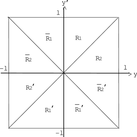
Figure 3: 8 regions

Step 1.Region R₁ and R₂

We start by solving (39) for the region $0\leq y,y^{\prime}\leq l$.
(i)$y\neq y^{\prime}$ .
In this case the equation (39) reduces to the homogeneous one.

$$(-{\tilde{p}}^{2}+\frac{\partial^{2}}{\partial y^{2}})G_{p}(y,y^{\prime})=(-{\tilde{p}}^{2}+\frac{\partial^{2}}{\partial{y^{\prime}}^{2}})G_{p}(y,y^{\prime})=0{\quad,}\quad{\tilde{p}}\equiv\sqrt{p^{2}}{\quad.}$$ (41)

The general solution is given by

$$K_{p}(y,y^{\prime})=A(y^{\prime})\cosh{\tilde{p}}y+B(y^{\prime})\sinh{\tilde{p}}y=C(y)\cosh{\tilde{p}}(y^{\prime}-l)+D(y)\sinh{\tilde{p}}(y^{\prime}-l){\quad,}$$ (42)

where $A(y^{\prime}),B(y^{\prime}),C(y)$ and $D(y)$ are to be fixed by the boundary conditions. We take the solution as

$$G_{p}(y,y^{\prime})=K_{p}(y,y^{\prime})=A(y^{\prime})\cosh{\tilde{p}}y+B(y^{\prime})\sinh{\tilde{p}}y\quad\mbox{for}\quad R_{1}\ :\ 0\leq y<y^{\prime}\leq l$$

$$G_{p}(y,y^{\prime})=K_{p}(y^{\prime},y)=C(y^{\prime})\cosh{\tilde{p}}(y-l)+D(y^{\prime})\sinh{\tilde{p}}(y-l)\quad\mbox{for}\quad R_{2}\ :\ 0\leq y^{\prime}<y\leq l\ ,$$ (43)

where we have used the sym(A) of (39). Note that the lower equation is the $y\leftrightarrow y^{\prime}$ exchanged one of the upper equation. This will be utilized in the inhomogeneous case below. Applying the b.c. (40) to the above result, we see

$$A(y^{\prime})=0{\quad,}\quad C(y)=0{\quad,}$$ (44)

in (42).

(ii) $|y-y^{\prime}|\ <\ +0$
We must take into accout the inhomogeous term, the singularity ${\frac{1}{2}}\delta(y-y^{\prime})$ in (39). To do it, we note the following fact. The absolute-value function ${\frac{1}{2}}|y-y^{\prime}|$ satisfies the following relation.

$$v(y,y^{\prime})\equiv{\frac{1}{2}}|y-y^{\prime}|=\left\{\begin{array}[]{ll}{\frac{1}{2}}(y^{\prime}-y)&\mbox{for}\ y<y^{\prime}\\ {\frac{1}{2}}(y-y^{\prime})=y\leftrightarrow y^{\prime}\mbox{ in the above}&\mbox{for}\ y>y^{\prime}\end{array}\right.{\quad,}$$ (47)

$$-\frac{\partial v(y,y^{\prime})}{\partial y}=+\frac{\partial v(y,y^{\prime})}{\partial y^{\prime}}={\frac{1}{2}}\epsilon(y^{\prime}-y)\equiv\left\{\begin{array}[]{ll}+{\frac{1}{2}}&\mbox{for}\quad y<y^{\prime}\\ 0&\mbox{for}\quad y=y^{\prime}\\ -{\frac{1}{2}}&\mbox{for}\quad y>y^{\prime}\end{array}\right.{\quad,}$$ (51)

$$\frac{\partial^{2}}{\partial y^{2}}v(y,y^{\prime})=\frac{\partial^{2}}{\partial{y^{\prime}}^{2}}v(y,y^{\prime})={\frac{1}{2}}\frac{\partial}{\partial y^{\prime}}\epsilon(y^{\prime}-y)=-{\frac{1}{2}}\frac{\partial}{\partial y}\epsilon(y^{\prime}-y)=\delta(y-y^{\prime}){\quad,}$$

$$\frac{\partial^{2}}{\partial y\partial y^{\prime}}v(y,y^{\prime})=-\delta(y-y^{\prime}){\quad,}$$ (52)

where $\epsilon(y)$ is the sign function. With the above relations and Sym(A) , we take the following b.c..

$$\mbox{Jump Condition:}\quad\left.\left[-\frac{\partial G_{p}(y,y^{\prime})}{\partial y}+\frac{\partial G_{p}(y,y^{\prime})}{\partial y^{\prime}}\right]\right|_{y^{\prime}\rightarrow y+0}={\frac{1}{2}}\quad\mbox{for}\quad y<y^{\prime}{\quad.}$$ (53)

(This b.c., in combined with the $y\leftrightarrow y^{\prime}$ exchanged definition for $y^{\prime}<y$ in (43), simply demands $G_{p}(y,y^{\prime})\sim+\frac{1}{4}|y-y^{\prime}|={\frac{1}{2}}v(y,y^{\prime})$ for $|y-y^{\prime}|\ll 1$. ) This condition and the continuity of the 2nd and 3rd equation of (42) at $y=y^{\prime}$ fix the remainig two functions $B$ and $D$. Finally we get

$$B(y^{\prime})=\frac{\sinh{\tilde{p}}(y^{\prime}-l)}{2{\tilde{p}}\sinh{\tilde{p}}l}{\quad,}\quad D(y)=\frac{\sinh{\tilde{p}}y}{2{\tilde{p}}\sinh{\tilde{p}}l}{\quad,}$$

$$G_{p}(y,y^{\prime})=\left\{\begin{array}[]{ll}{\frac{1}{2}}\sinh{\tilde{p}}y\sinh{\tilde{p}}(y^{\prime}-l)/{\tilde{p}}\sinh{\tilde{p}}l\equiv{\bar{K}}_{p}(y,y^{\prime})&\mbox{for}\quad 0\leq y<y^{\prime}\leq l\\ {\frac{1}{2}}\sinh{\tilde{p}}(y-l)\sinh{\tilde{p}}y^{\prime}/{\tilde{p}}\sinh{\tilde{p}}l\equiv{\bar{K}}_{p}(y^{\prime},y)&\mbox{for}\quad 0\leq y^{\prime}<y\leq l\end{array}\right.$$ (56)

We can view the result of Step 1 as follows. The solution for Region R₁ ($0\leq y<y^{\prime}\leq l$) can be expressed as

$${\bar{K}}_{p}(y,y^{\prime})=\sinh{\tilde{p}}y\sinh{\tilde{p}}(y^{\prime}-l)/2{\tilde{p}}\sinh{\tilde{p}}l$$

$$=\frac{1}{4{\tilde{p}}\sinh{\tilde{p}}l}\left[\{\cosh{\tilde{p}}(y^{\prime}+y)-\cosh{\tilde{p}}(y^{\prime}-y)\}\cosh{\tilde{p}}l\right.$$

$$\left.+\{-\sinh{\tilde{p}}(y^{\prime}+y)+\sinh{\tilde{p}}(y^{\prime}-y)\}\sinh{\tilde{p}}l\right]{\quad.}$$ (57)

As for the Region R₂, the solution is given by ${\bar{K}}_{p}(y^{\prime},y)$, which is given by changing $\sinh{\tilde{p}}(y^{\prime}-y)$ in (57) by $\sinh{\tilde{p}}(-y^{\prime}+y)$. In the combined region R₁ and R₂, this change is equivelent to change $\sinh{\tilde{p}}(y^{\prime}-y)$ by $\sinh{\tilde{p}}|y^{\prime}-y|$. This procedure of taking the absolute value of $(y^{\prime}-y)$, at the same time, makes the solution have the singularity $\delta(y-y^{\prime})$ and satisfy the inhomogeneous equation. (See eq.(52))

Here we stress the requirement of the exchange symmetry (A) and the $Z_{2}$ symmetry, with the Jump Condition (53), demand the delta-function source at the fixed point(s). We should compare this with the situation of the KK-expansion approach in Sec.2 and 3, where the singularity $\delta(y-y^{\prime})$ comes from the completeness of the eigen functions ${\hat{\delta}}(y-y^{\prime})\equiv\frac{1}{2l}\sum_{n\in{\bf Z}}\exp\{-i\frac{n\pi}{l}(y-y^{\prime})\}$. ( This situation is represented in the mathematical relation (59) derived below.)

Step 2.Extension to Region R${}_{1}^{\prime}$ and R${}_{2}^{\prime}$
 Here we extend the solution to Regions R${}_{1}^{\prime}$ and R${}_{2}^{\prime}$. We make use of the symmetry Sym(B). In order to make the solution (57)have the symmetry Sym(B), we must take the absolute value of $(y^{\prime}+y)$ in $-\sinh{\tilde{p}}(y^{\prime}+y)$ besides $(y^{\prime}-y)$ in $\sinh{\tilde{p}}(y^{\prime}-y)$.

$$G_{p}(y,y^{\prime})=\frac{1}{4{\tilde{p}}\sinh{\tilde{p}}l}\left[\{\cosh{\tilde{p}}|y^{\prime}+y|-\cosh{\tilde{p}}|y^{\prime}-y|\}\cosh{\tilde{p}}l\right.$$

$$\left.+\{-\sinh{\tilde{p}}|y^{\prime}+y|+\sinh{\tilde{p}}|y^{\prime}-y|\}\sinh{\tilde{p}}l\right]$$

$$=\frac{1}{4{\tilde{p}}\sinh{\tilde{p}}l}\{\cosh{\tilde{p}}(|y^{\prime}+y|-l)-\cosh{\tilde{p}}(|y^{\prime}-y|-l)\}{\quad.}$$ (58)

This expression is valid for $R_{1}^{\prime}$ and $R_{2}^{\prime}$ besides for $R_{1}$ and $R_{2}$.

Taking the limit ${\tilde{p}}\rightarrow+0$ in the above and (26), we obtain an interesting formula.

$$\sum_{n\in{\bf Z},n\neq 0}\frac{1}{({\frac{n\pi}{l}})^{2}}\sin{\frac{n\pi}{l}}y\sin{\frac{n\pi}{l}}y^{\prime}=\frac{1}{8l}\{(|y^{\prime}+y|-l)^{2}-(|y^{\prime}-y|-l)^{2}\}{\quad.}$$ (59)

In this $P=-1$ case, we can take the limit ${\tilde{p}}\rightarrow+0$ which means there is no massless mode.

Step 3.Extension to Region ${\bar{R}}_{1}$, ${\bar{R}}_{2}$ ${\bar{R}}_{1}^{\prime}$ and ${\bar{R}}_{2}^{\prime}$
 The solution (58) have the symmetries: Sym(C) ($y\rightarrow-y$) and Sym(C’) ($y^{\prime}\rightarrow-y^{\prime}$) with P=-1 property. These allow us to use (58) in all regions.

The appearance $|y^{\prime}+y|$ in (58) makes the solution have the singularity $\delta(y+y^{\prime})$ and satisfy the inhomogenous equation.

We notice, in this 5D propagator treatment, the extra coordinate behaves as a directed axis like the temperature. This is because the whole regions of ($y$,$y^{\prime}$)-plane reduces to the fundamental region $R_{1}(0\leq y<y^{\prime}\leq l)$. The property comes from the requirement of Z₂ symmetry (and the singularity at $y=\pm y^{\prime}$). Wave propagation in the continuum medium with the delta-function sources have a fixed direction in order to satisfy Z₂ symmetry.

For the time-like 4-momentum case, $p^{2}<0$, the solution is obtained in the same way and is given by

$$G_{p}(y,y^{\prime})=-\frac{1}{4{\hat{p}}\sin{\hat{p}}l}\left[\{\cos{\hat{p}}|y^{\prime}+y|-\cos{\hat{p}}|y^{\prime}-y|\}\cos{\hat{p}}l\right.$$

$$\left.+\{\sin{\hat{p}}|y^{\prime}+y|-\sin{\hat{p}}|y^{\prime}-y|\}\sin{\hat{p}}l\right]{\quad,}$$

$$=-\frac{1}{4{\hat{p}}\sin{\hat{p}}l}\left\{\cos{\hat{p}}(|y^{\prime}+y|-l)-\cos{\hat{p}}(|y^{\prime}-y|-l)\right\}{\quad,}$$ (60)

where ${\hat{p}}=\sqrt{-p^{2}}$.

Later, in Sec.9.1, we will show the graphs of (58) and of (60) and examine their behaviour.

4.2 Systematic treatment of symmetries of $G_{p}(y,y^{\prime})$

The defining equation of $G_{p}(y,y^{\prime})$, (39), has the symmetries Sym(A),(B),(C) and (C’). The fundamental region is R₁, and the solution in other regions can be expressed by some change of arguments $y,y^{\prime}$ in the P/M propagator in the fundamental region, ${\bar{K}}_{p}(y,y^{\prime})$.

In the previous subsection, we have done the procedure of taking the absolute value of $y^{\prime}-y$ for the singularity $\delta(y^{\prime}-y)$ and of $y^{\prime}+y$ for $\delta(y^{\prime}+y)$. This procedure says that the P/M propagator valid in all regions can be obtained by changing arguments $y,y^{\prime}$ in ${\bar{K}}_{p}(y,y^{\prime})$, which is the P/M propagator defined in the fundamental region $R_{1}$ and has no absolute-value quantities , in the following way.

$$y={\frac{1}{2}}(y+y^{\prime})-{\frac{1}{2}}(y^{\prime}-y)\rightarrow Y(y,y^{\prime})={\frac{1}{2}}|y+y^{\prime}|-{\frac{1}{2}}|y^{\prime}-y|=\left\{\begin{array}[]{ll}y&\mbox{for}\quad R_{1},\ {\bar{R}}_{1}\\ -y^{\prime}&\mbox{for}\quad{\bar{R}}_{2},\ R_{2}^{\prime}\\ -y&\mbox{for}\quad R_{1}^{\prime},\ {\bar{R}}_{1}^{\prime}\\ y^{\prime}&\mbox{for}\quad{\bar{R}}_{2}^{\prime},\ R_{2}\end{array}\right.$$ (65)

$$y^{\prime}={\frac{1}{2}}(y+y^{\prime})+{\frac{1}{2}}(y^{\prime}-y)\rightarrow Y^{\prime}(y,y^{\prime})={\frac{1}{2}}|y+y^{\prime}|+{\frac{1}{2}}|y^{\prime}-y|=\left\{\begin{array}[]{ll}y^{\prime}&\mbox{for}\quad R_{1},\ {\bar{R}}_{1}\\ -y&\mbox{for}\quad{\bar{R}}_{2},\ R_{2}^{\prime}\\ -y^{\prime}&\mbox{for}\quad R_{1}^{\prime},\ {\bar{R}}_{1}^{\prime}\\ y&\mbox{for}\quad{\bar{R}}_{2}^{\prime},\ R_{2}\end{array}\right.$$ (70)

Hence P/M propagator has the following form, for the space-like 4D momentum case, in each region.

$$\begin{array}[]{ll}{\bar{K}}_{p}(y,y^{\prime})=\frac{\sinh{\tilde{p}}y\sinh{\tilde{p}}(y^{\prime}-l)}{2{\tilde{p}}\sinh{\tilde{p}}l}&\mbox{for}\quad R_{1}\quad\mbox{and}\quad{\bar{R}}_{1}{\quad,}\\ {\bar{K}}_{p}(-y^{\prime},-y)=\frac{\sinh{\tilde{p}}y^{\prime}\sinh{\tilde{p}}(y+l)}{2{\tilde{p}}\sinh{\tilde{p}}l}&\mbox{for}\quad{\bar{R}}_{2}\quad\mbox{and}\quad R_{2}^{\prime}{\quad,}\\ {\bar{K}}_{p}(-y,-y^{\prime})=\frac{\sinh{\tilde{p}}y\sinh{\tilde{p}}(y^{\prime}+l)}{2{\tilde{p}}\sinh{\tilde{p}}l}&\mbox{for}\quad R_{1}^{\prime}\quad\mbox{and}\quad{\bar{R}}_{1}^{\prime}{\quad,}\\ {\bar{K}}_{p}(y^{\prime},y)=\frac{\sinh{\tilde{p}}y^{\prime}\sinh{\tilde{p}}(y-l)}{2{\tilde{p}}\sinh{\tilde{p}}l}&\mbox{for}\quad{\bar{R}}_{2}^{\prime}\quad\mbox{and}\quad R_{2}{\quad.}\\ \end{array}$$ (75)

In Fig.4, the arrangement of above propagators is shown.

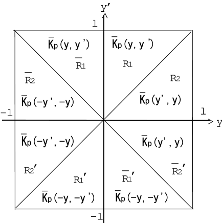
Figure 4: Arguments Arrangement for Propagators in 8 regions. The explicit expressions are given in (75).

We surely see the symmetries (A),(B),(C) and (C’) are satisfied. Using the new variables $Y(y,y^{\prime}),Y^{\prime}(y,y^{\prime})$ , the solution (58) (space-like momentum case) is equivalently expressed as

$$G_{p}(y,y^{\prime})={\bar{K}}_{p}(Y(y,y^{\prime}),Y^{\prime}(y,y^{\prime})){\quad,}$$ (76)

where ${\bar{K}}_{p}$ is given in (57). For the time-like case, ${\bar{K}}_{p}$ is given by ${\bar{K}}_{p}(Y,Y^{\prime})=\frac{\sin{\hat{p}}Y\sin{\hat{p}}(Y^{\prime}-l)}{2{\hat{p}}\sin{\hat{p}}l},{\hat{p}}=\sqrt{-p^{2}}$.

As for the periodic property and the extension to $-\infty<y<\infty$, we examine in the next section.

We have given the P/M propagator in the flat 5D scalar theory (with $P=-1$) in the two ways: (1) eq.(58) or eq.(60) (compactly by (76)) where absolute functions appear, and this expression is valid for all regions; (2) eq.(75) where no absolute-value function appears and the arguments within ${\bar{K}}_{p}$ change depending on each region. Both ways are important. The first way is indispensable for analyzing the propagator at singular points. Practically it is necessary to draw a graph which has singular behaviour, while the second one stresses the importance of $Z_{2}$-symmetry. (See the $\delta(0)$-problem in Sec.10.)

5 KK-expansion approach versus P/M propagator approach

We have examined the same propagator equation (27) and (38) in two approaches. One is utilizing the expansion with the eigen functions (KK-modes) of $\exp(i{\frac{n\pi}{l}}x^{5})$. The other makes use of the P/M propagator $G_{p}(y,y^{\prime})$ in (39). In the former, the extra space is R=($-\infty<x^{5}<\infty$) and the periodic b.c. and $Z_{2}$ symmetry are imposed. The 4D space-time propagator is Feynman’s. Ths is the orbifold approach. In the latter case, the extra space is the interval $[-l,l]$. $Z_{2}$ symmetry only is imposed. This is the interval approach. We now connect the two results.

The P/M propagator for $0\leq y<y^{\prime}\leq l$ (Region $R_{1}$)is given by

$${\bar{K}}_{p}(y,y^{\prime})=$$

$$\left\{\begin{array}[]{ll}\frac{\sinh{\tilde{p}}y\sinh{\tilde{p}}(y^{\prime}-l)}{2{\tilde{p}}\sinh{\tilde{p}}l}=\frac{1}{4{\tilde{p}}\sinh{\tilde{p}}l}\{\cosh{\tilde{p}}(y^{\prime}+y-l)-\cosh{\tilde{p}}(y^{\prime}-y-l)\}\ ,\ {\tilde{p}}=\sqrt{p^{2}}&\mbox{for}\quad p^{2}>0\\ \frac{\sin{\hat{p}}y\sin{\hat{p}}(y^{\prime}-l)}{2{\hat{p}}\sin{\hat{p}}l}=\frac{1}{4{\hat{p}}\sin{\hat{p}}l}\{-\cos{\hat{p}}(y^{\prime}+y-l)+\cos{\hat{p}}(y-y^{\prime}+l)\}\ ,\ {\hat{p}}=\sqrt{-p^{2}}&\mbox{for}\quad p^{2}<0\end{array}\right.$$ (79)

Using the Fourier expansion formulae,

$$\frac{\pi}{2a}\frac{\cosh a(\pi-x)}{\sinh a\pi}=\frac{1}{2a^{2}}+\sum_{n=1}^{\infty}\frac{\cos nx}{n^{2}+a^{2}},\ 0\leq x\leq 2\pi,\ a:\ \mbox{arbitrary constant.}$$

$$\frac{\pi}{2a}\frac{\cos ax}{\sin a\pi}=\frac{1}{2a^{2}}+\sum_{n=1}^{\infty}(-1)^{n-1}\frac{\cos nx}{n^{2}-a^{2}},\ -\pi\leq x\leq\pi,\ a:\ \mbox{non-integer arbitrary constant.}$$ (80)

we obtain

$${\bar{K}}_{p}(y,y^{\prime})=\left\{\begin{array}[]{ll}-\frac{1}{l}\sum_{n=1}^{\infty}\frac{1}{{\tilde{p}}^{2}+({\frac{n\pi}{l}})^{2}}\sin{\frac{n\pi}{l}}y\sin{\frac{n\pi}{l}}y^{\prime}&\mbox{for}\quad p^{2}>0\\ \frac{1}{l}\sum_{n=1}^{\infty}\frac{1}{{\hat{p}}^{2}-({\frac{n\pi}{l}})^{2}}\sin{\frac{n\pi}{l}}y\sin{\frac{n\pi}{l}}y^{\prime}&\mbox{for}\quad p^{2}<0\end{array}\right.$$ (83)

This propagator satisfies the all symmetries (A),(B),(C) and (C’) and is periodic ($y\rightarrow y+2l$), hence we may take it as the propagator valid for $y,y^{\prime}\in$R where R=$(-\infty,\infty)$. The last procedure is taking the universal covering of $S_{1}$. Both the space-like case and the time-like case are just the result (26) with $P=-1$.

We reemphasize the following points. In the periodic approach of Sec.2, the delta function singularity comes from the completeness of the eigen-functions ${\rm e}^{in\pi y/l}$. In the interval approach of Sec.4, the singularity comes from the exchange symmetry (A) and Z₂-symmetry (, that is, taking the absolute values of ($y\mp y^{\prime}$)). The position space treatment gives the intimate relation between the wave propagation with symmetries and its source (singularity).

6 5D QFT on warped geometry AdS₅

Let us consider the warped case. The space-time is AdS₅ manifold.

$$ds^{2}={\rm e}^{-2\sigma(y)}\eta_{ab}dx^{a}dx^{b}+dy^{2}{\quad,}\quad-\infty<y<\infty{\quad,}$$

$$(\eta_{ab})=\mbox{diag}(-1,1,1,1){\quad,}\quad\sigma(y)=\omega|y|{\quad,}\quad\omega>0$$ (84)

The manifold has the negative cosmological constant and is maximally symmetric with the curvature $\omega$. In the limit $\omega\rightarrow 0$, the line element (84) goes to the flat one of Sec.2. We can consider the symmetries.

(1) Periodicity

$y\rightarrow y+2l$

(2) Z₂-property

$y\leftrightarrow-y$, $P=\pm$ 1

as in Sec.2. When the periodicity condition (1) is assumed, $|y|$ in (84) is the periodic absolute-linear function[18]. Instead of $y$-coordinate, another one $z$, defined below, is also important.

$$z=\left\{\begin{array}[]{ll}\frac{1}{\omega}{\rm e}^{\omega y}&\mbox{for}\quad y>0\\ &\\ \ 0&\mbox{for}\quad y=0\\ &\\ -\frac{1}{\omega}{\rm e}^{-\omega y}&\mbox{for}\quad y<0\end{array}\right.\quad\quad=\ \epsilon(y)\frac{{\rm e}^{\omega|y|}}{\omega}$$ (90)

See Fig.5.

Figure 5: Relation between coordinates $z$ and $y$

In terms of $z$, the metric can be expressed as

$$ds^{2}=\frac{1}{\omega^{2}z^{2}}(\eta_{ab}dx^{a}dx^{b}+(dz)^{2}){\quad,}\quad z>\frac{1}{\omega}\ \mbox{or}\ z<-\frac{1}{\omega}{\quad,}$$

$$\frac{dz}{\omega z}=\left\{\begin{array}[]{ll}dy&\mbox{for}\quad y>0\\ -dy&\mbox{for}\quad y<0\end{array}\right.$$ (93)

$(-\frac{1}{\omega},0)$U$(0,\frac{1}{\omega})$ is the ’prohibited’ region whose values the z-coordinate cannot take. This metric is conformal flat.

The advantage of the choice (90) is as follows: (a) $z$ is the monotonously increasing function of $y$; (b) one-to-one ; (c) the $Z_{2}$ symmetry is expressed in the same way as $y$.

(2’) Z₂-property

$z\leftrightarrow-z$, $P=\pm$ 1

The periodicity is expressed as

(1’) Periodicity $y\rightarrow y+2l$

$z\rightarrow z{\rm e}^{2\omega l}(>0)$	for  $z>\frac{1}{\omega}$
$z=0\rightarrow z=\frac{{\rm e}^{2\omega l}}{\omega}=\frac{\omega}{T^{2}}$	for  $z=0$
$z(<0)\rightarrow-z{\rm e}^{2\omega l}(>0)$	for  $-\frac{\omega}{T^{2}}=-\frac{{\rm e}^{2\omega l}}{\omega}<z<-\frac{1}{\omega}$
$z=-\frac{{\rm e}^{2\omega l}}{\omega}=-\frac{\omega}{T^{2}}\rightarrow z=0$	for  $z=-\frac{{\rm e}^{2\omega l}}{\omega}=-\frac{\omega}{T^{2}}$
$z\rightarrow z{\rm e}^{-2\omega l}(<0)$	for  $z<-\frac{{\rm e}^{2\omega l}}{\omega}=-\frac{\omega}{T^{2}}$

The translation in $y$-coordinate is the scale transformation in $z$-coordinate. In the conformal coordinate (93), we can not obtain the flat limit simply by $\omega\rightarrow 0$.

We take 5D massive scalar theory as a simple example. The Lagrangian and the field equation is written as

$${\cal L}=\sqrt{-G}(-{\frac{1}{2}}\nabla^{A}\Phi\nabla_{A}\Phi-{\frac{1}{2}}m^{2}\Phi^{2}+J\Phi){\quad,}\quad G\equiv\det G_{AB}{\quad,}$$

$$ds^{2}=G_{AB}dX^{A}dX^{B}{\quad,}\quad\nabla^{A}\nabla_{A}\Phi-m^{2}\Phi+J=0{\quad,}$$ (94)

where $\Phi(X)=\Phi(x^{a},z)$ is the 5D scalar field and $J(X)=J(x^{a},z)$ is the external source field. The background geometry is AdS₅ which takes the following form, in terms of $z$,

$$(G_{AB})=\left(\begin{array}[]{ll}\frac{1}{\omega^{2}z^{2}}\eta_{ab}&0\\ 0&\frac{1}{\omega^{2}z^{2}}\end{array}\right){\quad,}\quad\sqrt{-G}=\frac{1}{(\omega|z|)^{5}}$$ (97)

$$-\frac{1}{T}\leq z\leq-\frac{1}{\omega}\quad\mbox{or}\quad\frac{1}{\omega}\leq z\leq\frac{1}{T}\quad(-l\leq y\leq l){\quad,}\quad\frac{1}{T}\equiv\frac{1}{\omega}{\rm e}^{\omega l}{\quad,}$$ (98)

where, at present, we take into account only $Z_{2}$ symmetry in the interval $y\in[-l,\ l]$. Later we will discuss the periodicity condition. The field equation (94) leads to

$$\omega^{2}z^{2}\partial_{a}\partial^{a}\Phi+(\omega z)^{5}\partial_{z}(\frac{1}{(\omega z)^{3}}\partial_{z}\Phi)-m^{2}\Phi+J=0{\quad,}$$ (99)

which is $Z_{2}$-symmetric. We can consider two cases:

$$\Phi(x,z)=P\Phi(x,-z){\quad,}\quad J(x,z)=PJ(x,-z){\quad,}$$

$$P=+1\ (\mbox{even}){\quad,}\quad P=-1\ (\mbox{odd}){\quad,}$$ (100)

Let us first solve the above equation by the KK-expansion method as in Sec.2.

$$\Phi(x^{a},z)=\sum_{n}\phi_{n}(x)\psi_{n}(z){\quad,}\quad J(x^{a},z)=\sum_{n}j_{n}(x)\psi_{n}(z){\quad,}\quad\psi_{n}(z)=\mbox{P}\psi_{n}(-z){\quad,}\quad\mbox{P}=\mp 1\ ,$$ (101)

where $\psi_{n}(z)$ is the eigen-functions of the Bessel differential equation. The variable region of $z$ is the intervals defined in (98).

$$(\omega z)^{3}\partial_{z}(\frac{1}{(\omega z)^{3}}\partial_{z}\psi_{n})-\frac{m^{2}}{(\omega z)^{2}}\psi_{n}=-M_{n}^{2}\psi_{n}$$

$$(\int^{-\frac{1}{\omega}}_{-\frac{1}{T}}+\int_{\frac{1}{\omega}}^{\frac{1}{T}})\frac{dz}{(\omega|z|)^{3}}\psi_{n}(z)\psi_{k}(z)=2\int_{\frac{1}{\omega}}^{\frac{1}{T}}\frac{dz}{(\omega z)^{3}}\psi_{n}(z)\psi_{k}(z)=\delta_{nk}{\quad,}$$ (102)

where $M_{n}$ is the eigenvalues to be determined by the b.c.. The above equation is obtained by the requirement that the 4D field $\phi_{n}(x),\ j_{n}(x)$ in (101) satisfy the ordinary massive scalar field equation.

$$\partial_{a}\partial^{a}\phi_{n}-M_{n}^{2}\phi_{n}+j_{n}=0{\quad.}$$ (103)

From eq.(101), $\psi_{n}(z)$ are odd or even functions of $z$. $z$ varies in $-1/T\leq z\leq-1/\omega$ and $1/\omega\leq z\leq 1/T$. Hence instead of ordinary Bessel functions $({\bf J}_{\nu}(z),{\bf N}_{\nu})$ where $z>0$, it is better to introduce odd or even Bessel functions where the argument $z$ is valid even for the negative region of $z$. It can be done as follows because the Bessel equation is invariant for $Z_{2}$ symmetry: $z\rightarrow-z$.

$$\begin{array}[]{lll}\tilde{\bf J}_{\nu}(z)\equiv\epsilon(z){\bf J}_{\nu}(|z|)&\tilde{\bf N}_{\nu}(z)\equiv\epsilon(z){\bf N}_{\nu}(|z|)&\mbox{for P=}-1\\ \hat{\bf J}_{\nu}(z)\equiv{\bf J}_{\nu}(|z|)&\hat{\bf N}_{\nu}(z)\equiv{\bf N}_{\nu}(|z|)&\mbox{for P=1}\end{array}$$ (106)

where $\epsilon(z)$ is the sign function introduced in(52). Taking the case P=$-1$, eq.(102) has two "intermediate" solutions.

$$\varphi^{(1/\omega)}(z) = \frac{(\omega z)^{2}}{N^{(1/\omega)}}\left[\tilde{\bf J}_{\nu}(Mz)+b_{\nu}(M)\tilde{\bf N}_{\nu}(Mz)\right],$$ (107)

$$\varphi^{(1/T)}(z) = \frac{(\omega z)^{2}}{N^{(1/T)}}\left[\tilde{\bf J}_{\nu}(Mz)+b_{\nu}(\omega M/T)\tilde{\bf N}_{\nu}(Mz)\right],$$ (108)

where $N^{(1/\omega)}$ and $N^{(1/T)}$ are some normalization constants to be determined. Similarly for the case P=1. $b_{\nu}$ is given by

$$b_{\nu}(t) \equiv \left\{\begin{array}[]{c}-\mbox{{\bf J}}_{\nu}(t/\omega)/\mbox{{\bf N}}_{\nu}(t/\omega),\quad\mbox{for}\ P=-1,\\ -\mbox{{\bf J}}^{\prime}_{\nu}(t/\omega)/\mbox{{\bf N}}^{\prime}_{\nu}(t/\omega),\quad\mbox{for}\ P=1,\end{array}\right.$$ (111)

and

$$\nu=\sqrt{4+\frac{m^{2}}{\omega^{2}}}.$$ (112)

These solutions $\varphi^{(1/\omega)}(z)$ and $\varphi^{(1/T)}(z)$ satisfy the following boundary conditions at $z=\frac{1}{\omega}$ and $\frac{1}{T}$, respectively.

$$\begin{array}[]{cccc}\mbox{Dirichlet b.c.}&\varphi^{(1/\omega)}(z)|_{z=1/\omega}=0&\varphi^{(1/T)}(z)|_{z=1/T}=0&\mbox{for}\quad P=-1\\ \mbox{Neumann b.c.}&\left.\frac{d}{dz}\varphi^{(1/\omega)}(z)\right|_{z=1/\omega}=0&\left.\frac{d}{dz}\varphi^{(1/T)}(z)\right|_{z=1/T}=0&\mbox{for}\quad P=1\end{array}$$ (115)

The "final" solution which satisfies the b.c. both at $z=1/\omega$ and $z=1/T$ is obtained by the condition that these two solutions are not independent.

$$b_{\nu}(M_{n}) = b_{\nu}(\omega M_{n}/T)\equiv b_{\nu}^{(n)},$$

$$\begin{array}[]{c}\frac{\mbox{{\bf J}}_{\nu}(\frac{{M_{n}}}{\omega})}{\mbox{{\bf N}}_{\nu}(\frac{{M_{n}}}{\omega})}=\frac{\mbox{{\bf J}}_{\nu}(\frac{{M_{n}}}{T})}{\mbox{{\bf N}}_{\nu}(\frac{{M_{n}}}{T})},\quad\mbox{for}\ P=-1,\\ \frac{\mbox{{\bf J}}_{\nu}^{\prime}(\frac{{M_{n}}}{\omega})}{\mbox{{\bf N}}_{\nu}^{\prime}(\frac{{M_{n}}}{\omega})}=\frac{\mbox{{\bf J}}_{\nu}^{\prime}(\frac{{M_{n}}}{T})}{\mbox{{\bf N}}_{\nu}^{\prime}(\frac{{M_{n}}}{T})},\quad\mbox{for}\ P=1,\end{array}$$ (118)

which makes them identified,

$$\left.\varphi^{(1/\omega)}(z)\right|_{M=M_{n}}=\left.\varphi^{(1/T)}(z)\right|_{M=M_{n}}\equiv\psi_{n}(z),$$ (119)

and determines the eigenvalues $M_{n}$. The normalization constants are then expressed as

$$N_{n}^{(1/\omega)2} = N_{n}^{(1/T)2}=\int^{1/T}_{1/\omega}\omega zdz\left[\mbox{{\bf J}}_{\nu}(M_{n}z)+b_{\nu}^{(n)}\mbox{{\bf N}}_{\nu}(M_{n}z)\right]^{2}\equiv N_{n}^{2}.$$ (120)

The solution of (103) is given by

$$\phi_{n}(x)=\int\Delta_{F}^{n}(x-x^{\prime})j_{n}(x^{\prime})d^{4}x^{\prime}{\quad,}\quad\Delta_{F}^{n}(x-x^{\prime})={\int\frac{d^{4}k}{(2\pi)^{4}}}\frac{{\rm e}^{-ik(x-x^{\prime})}}{k^{2}+M_{n}^{2}-i\epsilon}{\quad,}$$

$$(\partial_{a}\partial^{a}-M_{n}^{2})\Delta_{F}^{n}(x-x^{\prime})=-\delta^{4}(x-x^{\prime}){\quad.}$$ (121)

5D propagator can be expected to be , in the analogy of Sec.2’s result (26),

$$\Phi(X)=\int d^{5}X^{\prime}\Delta_{W}(X,X^{\prime})\sqrt{-G^{\prime}}J(X^{\prime}){\quad,}$$

$$\Delta_{W}(X,X^{\prime})\equiv\sum_{n}\Delta_{F}^{n}(x-x^{\prime})\times{\frac{1}{2}}\{\psi_{n}(z)\psi_{n}(z^{\prime})+P\psi_{n}(z)\psi_{n}({\tilde{z}}^{\prime})\}{\quad,}\quad{\tilde{z}}^{\prime}\equiv-z^{\prime}{\quad.}$$ (122)

In fact we can confirm the following propagator equation.

$$(\nabla^{A}\nabla_{A}-m^{2})\Delta_{W}(X,X^{\prime})=\{\omega^{2}z^{2}\partial_{a}\partial^{a}+(\omega z)^{5}\frac{\partial}{\partial z}\frac{1}{(\omega z)^{3}}\partial_{z}-m^{2}\}\Delta_{W}(X.X^{\prime})$$

$$=\sum_{n}\omega^{2}z^{2}(\partial_{a}\partial^{a}-M_{n}^{2})\Delta_{F}^{n}(x-x^{\prime}){\frac{1}{2}}\{\psi_{n}(z)\psi_{n}(z^{\prime})+P\psi_{n}(z)\psi_{n}({\tilde{z}}^{\prime})\}$$

$$=-(\omega|z|)^{5}\delta^{4}(x-x^{\prime}){\frac{1}{2}}({\hat{\delta}}(z-z^{\prime})+P{\hat{\delta}}(z-{\tilde{z}}^{\prime})){\quad,}$$ (123)

where some relations in (102), (121) and the completeness relation:

$$(\omega|z|)^{-3}\sum_{n}\psi_{n}(z)\psi_{n}(z^{\prime})\equiv\left\{\begin{array}[]{ll}\epsilon(z)\epsilon(z^{\prime}){\hat{\delta}}(|z|-|z^{\prime}|)&\mbox{for\ \ P=}-1\\ {\hat{\delta}}(|z|-|z^{\prime}|)&\mbox{for\ \ P=}1\end{array}\right.{\quad,}$$ (126)

are used.

Now we have obtained 5D propagator $\Delta_{W}(x^{a},y;{x^{\prime}}^{a},y^{\prime})$ which satisfies $Z_{2}$ symmetry and is valid for $y,y^{\prime}\in[-l,l]$. When we want to extend this to $y,y^{\prime}\in\mbox{{\bf R}}$ and impose the periodicity, we may take the universal covering of $\Delta_{W}(x^{a},y;{x^{\prime}}^{a},y^{\prime})$ as in the flat case. That is, first we Fourier-expand $\Delta_{W}(x^{a},y;{x^{\prime}}^{a},y^{\prime})$ within $y,y^{\prime}\in[-l,l]$, and then, confirming the non-singular behaviour, extend the variable region to R.

The above relations can be expressed in the Dirac’s bra and ket vector formalism. Let us introduce bra and ket vectors as follows.

$$\psi_{n}(z)\equiv(n|z)=(z|n){\quad,}\quad{\rm e}^{-ikx}\equiv<x|k>{\quad,}\quad{\rm e}^{ikx}\equiv<k|x>{\quad,}$$ (127)

Depending on the Z₂-property of $\psi_{n}(z)$, $|z)$ and $(z|$ have the following properties.

$$|-z)=P|z){\quad,}\quad(-z|=P(z|{\quad,}\quad P=\mp 1{\quad.}$$ (128)

From the orthogonality relation (102), we know

$$\left(\int_{-\frac{1}{T}}^{-\frac{1}{\omega}}+\int_{\frac{1}{\omega}}^{\frac{1}{T}}\right)\frac{dz}{(\omega|z|)^{3}}(n|z)(z|k)=2\int_{\frac{1}{\omega}}^{\frac{1}{T}}\frac{dz}{(\omega z)^{3}}(n|z)(z|k)=\delta_{n,k}{\quad.}$$ (129)

We require the orthogonality between $(n|$ and $|k)$,

$$(n|k)=\delta_{n,k}{\quad.}$$ (130)

then the completeness relation between the coordinate states $|z)$

$$\left(\int_{-\frac{1}{T}}^{-\frac{1}{\omega}}+\int_{\frac{1}{\omega}}^{\frac{1}{T}}\right)\frac{dz}{(\omega|z|)^{3}}|z)(z|=2\int_{\frac{1}{\omega}}^{\frac{1}{T}}\frac{dz}{(\omega z)^{3}}|z)(z|={\bf 1}{\quad.}$$ (131)

is deduced.

The completeness relation (126) is expressed as

$$\sum_{n}(z|n)(n|z^{\prime})=\left\{\begin{array}[]{ll}(\omega|z|)^{3}\epsilon(z)\epsilon(z^{\prime}){\hat{\delta}}(|z|-|z^{\prime}|)&\mbox{for\ \ P=}-1\\ (\omega|z|)^{3}{\hat{\delta}}(|z|-|z^{\prime}|)&\mbox{for\ \ P=}1\end{array}\right.{\quad.}$$ (134)

If we require the orthogonality between the coordinate states $(z|$ and $|z^{\prime})$:

$$(z|z^{\prime})=\left\{\begin{array}[]{ll}(\omega|z|)^{3}\epsilon(z)\epsilon(z^{\prime}){\hat{\delta}}(|z|-|z^{\prime}|)&\mbox{for\ \ P=}-1\\ (\omega|z|)^{3}{\hat{\delta}}(|z|-|z^{\prime}|)&\mbox{for\ \ P=}1\end{array}\right.{\quad,}$$ (137)

then the completeness:

$$\sum_{n}|n)(n|={\bf 1}{\quad,}$$ (138)

is deduced. The 5D propagator (122) can be expressed as

$$\Delta_{W}(X,X^{\prime})=\sum_{n}{\int\frac{d^{4}k}{(2\pi)^{4}}}\frac{<x|k><k|x^{\prime}>}{k^{2}+M_{n}^{2}-i\epsilon}\times{\frac{1}{2}}\{(z|n)(n|z^{\prime})+P(z|n)(n|{\tilde{z}}^{\prime})\}$$

$$=2l\int d^{5}K{\frac{1}{2}}\{\frac{(X|K)(K|X^{\prime})+P(X|K)(K|{\tilde{X}}^{\prime})}{K^{2}-i\epsilon}\}{\quad,}$$

$$(X)\equiv(x^{a},z){\quad,}\quad(X^{\prime})\equiv({x^{a}}^{\prime},z^{\prime}){\quad,}\quad({\tilde{X}}^{\prime})\equiv({x^{a}}^{\prime},-z^{\prime}){\quad,}$$

$$(K)\equiv(k_{a},M_{n}){\quad,}\quad\int d^{5}K\equiv\frac{1}{2l}\sum_{n}{\int\frac{d^{4}k}{(2\pi)^{4}}}{\quad.}$$ (139)

where 5D bra and ket vectors are introduced as

$$(X|K)\equiv<x|k>(z|n){\quad,}\quad(K|X^{\prime})\equiv<k|x^{\prime}>(n|z^{\prime}){\quad.}$$ (140)

This is the same form as in the flat case of Sec.3. The generalized points are the appearance of the extra-space ’measure factor’ $(\omega|z|)^{-3}$ in (129), (131), (134), (137) and, in the extra dimensional part, the periodic eigen functions are replaced by the Bessel ones $(n|z)=(z|n)=\psi_{n}(z)$.

In this section we have shown the basic quantum structure of the warped system, in the Dirac’s bra and ket vector formalism, is the same as the flat one. In this sense, the warped system can be regarded as a deformation of the flat theory with the deformation parameter $\omega$. We will again point out the same interpretation from the propagator behaviour in Sec.10.

7 P/M Propagator approach to 5D QFT on AdS₅

Let us solve the field equation (99) in the P/M propagator approach.

$$\nabla^{A}\nabla_{A}\Phi-m^{2}\Phi+J=$$

$$\omega^{2}z^{2}\partial_{a}\partial^{a}\Phi+(\omega z)^{5}\partial_{z}(\frac{1}{(\omega z)^{3}}\partial_{z}\Phi)-m^{2}\Phi+J=0{\quad.}$$ (141)

We consider the Z₂-parity odd case:

$$\mbox{Z${}_{2}$-property (5D parity)}\quad\quad\Phi(x,z)=\mbox{P}\Phi(x,-z)\ ,\ J(x,z)=\mbox{P}J(x,-z){\quad,}\quad P=-1{\quad,}$$ (142)

The P/M propagator $G_{p}(z,z^{\prime})$ is introduced as

$$\Phi(X)=\int d^{5}X^{\prime}\Delta_{W}(X,X^{\prime})\sqrt{-G^{\prime}}J(X^{\prime}){\quad,}\quad$$

$$(\nabla^{A}\nabla_{A}-m^{2})\Delta_{W}(X,X^{\prime})=-\frac{1}{\sqrt{-G}}\delta^{4}(x-x^{\prime}){\frac{1}{2}}(\delta(z-z^{\prime})+P\delta(z-{\tilde{z}}^{\prime})){\quad,}\quad P=-1{\quad,}$$

$$\Delta_{W}(X,X^{\prime})={\int\frac{d^{4}p}{(2\pi)^{4}}}{\rm e}^{ip(x-x^{\prime})}G_{p}(z,z^{\prime}){\quad,}$$ (143)

where $(X^{A})=(x^{a},z),({X^{A}}^{\prime})=({x^{a}}^{\prime},z^{\prime})$ and $G=\mbox{det}G_{AB}$. In Sec.6, we have derived $\Delta_{W}$ in the KK-expansion approach. Here we rederive it in the P/M propagator approach. From the propagator equation above, $G_{p}(z,z^{\prime})$ must satisfy

$$\{-\omega^{2}z^{2}p^{2}+(\omega z)^{5}\frac{\partial}{\partial z}\frac{1}{(\omega z)^{3}}\partial_{z}-m^{2}\}G_{p}(z,z^{\prime})$$

$$=-{\frac{1}{2}}(\omega|z|)^{5}(\delta(z-z^{\prime})+P\delta(z-{\tilde{z}}^{\prime})){\quad,}$$ (144)

(The absolute value $|z|$ comes from the space-time volume measure $\sqrt{-G}=\sqrt{-\mbox{det}G_{AB}}$.) Hence $G_{p}$ is determined by the Bessel differential equation.

$$\{-p^{2}+{\partial_{z}}^{2}-\frac{3}{z}\partial_{z}-\frac{m^{2}}{\omega^{2}z^{2}}\}G_{p}(z,z^{\prime})=-{\frac{1}{2}}(\omega|z|)^{3}(\delta(z-z^{\prime})+P\delta(z-{\tilde{z}}^{\prime})){\quad,}$$

$$-\frac{1}{T}\leq z,z^{\prime}\leq-\frac{1}{\omega}\quad\mbox{or}\quad\frac{1}{\omega}\leq z,z^{\prime}\leq\frac{1}{T}\$$ (146)

The above equation has the symmetries.

Sym(A)

$z\leftrightarrow z^{\prime}$

Sym(B)

$z\rightarrow-z\ \mbox{and}\ z^{\prime}\rightarrow-z^{\prime}$ , $P=(-1)\times(-1)=1$

Sym(C)

$z\rightarrow-z$ , $P=-1$

Sym(C’)

$z^{\prime}\rightarrow-z^{\prime}$ , $P=-1$

Corresponding to the choice of $P=-1$ in (142), we take the Dirichlet b.c. at the fixed points: $z,z^{\prime}=\pm\frac{1}{\omega},\ \pm\frac{1}{T}$. Now let us solve (146) in the same way as in Sec.4. We consider $p^{2}>0$ (space-like) case first.

We divide the whole region into 8 ones, $R_{1},R_{2},R_{1}^{\prime},R_{2}^{\prime},{\bar{R}}_{1},{\bar{R}}_{2},{\bar{R}}_{1}^{\prime}$ and ${\bar{R}}_{2}^{\prime}$ as in Fig.6.

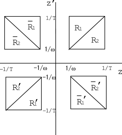
Figure 6: 8 regions in the z-coordinates plane. This is the transformed version of Fig.3 through the relation (90)

Step 1.Region R₁ and R₂

We start by solving (146) for the region $\frac{1}{\omega}\leq z,z^{\prime}\leq\frac{1}{T}$.
(i)$z\neq z^{\prime}$ .
In this case the equation (146) reduces to the homogeneous one.

$$(-{\tilde{p}}^{2}+{\partial_{z}}^{2}-\frac{3}{z}\partial_{z}-\frac{m^{2}}{\omega^{2}z^{2}})G_{p}(z,z^{\prime})$$

$$=(-{\tilde{p}}^{2}+{\partial_{z^{\prime}}}^{2}-\frac{3}{z^{\prime}}\partial_{z^{\prime}}-\frac{m^{2}}{\omega^{2}{z^{\prime}}^{2}})G_{p}(z,z^{\prime})=0{\quad,}\quad{\tilde{p}}\equiv\sqrt{p^{2}}{\quad.}$$ (147)

The general solution is given by

$$K_{p}(z,z^{\prime})=A(z^{\prime})z^{2}{\bf K}_{\nu}({\tilde{p}}z)+B(z^{\prime})z^{2}{\bf I}_{\nu}({\tilde{p}}z)=C(z){z^{\prime}}^{2}{\bf K}_{\nu}({\tilde{p}}z^{\prime})+D(z){z^{\prime}}^{2}{\bf I}_{\nu}({\tilde{p}}z^{\prime}){\quad,}$$

$$\nu=\sqrt{4+\frac{m^{2}}{\omega^{2}}}$$ (148)

where $A(z^{\prime}),B(z^{\prime}),C(z)$ and $D(z)$ are to be fixed by the boundary conditions. We consider the special case which is important in the supersymmetry requirement[19].

$$m^{2}=-4\omega^{2}{\quad,}\quad\nu=0{\quad.}$$ (149)

We take the solution as

$$G_{p}(z,z^{\prime})=K_{p}(z,z^{\prime})=A(z^{\prime})z^{2}{\bf K}_{0}({\tilde{p}}z)+B(z^{\prime})z^{2}{\bf I}_{0}({\tilde{p}}z)=C(z){z^{\prime}}^{2}{\bf K}_{0}({\tilde{p}}z^{\prime})+D(z){z^{\prime}}^{2}{\bf I}_{0}({\tilde{p}}z^{\prime}){\quad,}$$

$$\mbox{for}\quad\frac{1}{\omega}\leq z<z^{\prime}\leq\frac{1}{T}$$

$$G_{p}(z,z^{\prime})=K_{p}(z^{\prime},z)=A(z){z^{\prime}}^{2}{\bf K}_{0}({\tilde{p}}z^{\prime})+B(z){z^{\prime}}^{2}{\bf I}_{0}({\tilde{p}}z^{\prime})=C(z^{\prime}){z}^{2}{\bf K}_{0}({\tilde{p}}z)+D(z^{\prime}){z}^{2}{\bf I}_{0}({\tilde{p}}z){\quad,}$$

$$\mbox{for}\quad\frac{1}{\omega}\leq z^{\prime}<z\leq\frac{1}{T}{\quad.}$$ (150)

The latter equation is the $z\leftrightarrow z^{\prime}$ exchanged one of the former equation. Here we use Sym.(A). The Dirichlet b.c. requires

$$A(z^{\prime}){\bf K}_{0}(\frac{{\tilde{p}}}{\omega})+B(z^{\prime}){\bf I}_{0}(\frac{{\tilde{p}}}{\omega})=0{\quad,}$$

$$C(z^{\prime}){\bf K}_{0}(\frac{{\tilde{p}}}{T})+D(z^{\prime}){\bf I}_{0}(\frac{{\tilde{p}}}{T})=0{\quad.}$$ (151)

(ii) $|z-z^{\prime}|\ <\ +0$
In order to take into account the inhomogeneous term $-{\frac{1}{2}}(\omega|z|)^{3}\delta(z-z^{\prime})$ in the RHS of (146) we put the following b.c..

$$\mbox{Jump Condition:}\quad\left.-\frac{\partial G_{p}(z,z^{\prime})}{\partial z}+\frac{\partial G_{p}(z,z^{\prime})}{\partial z^{\prime}}\right|_{z^{\prime}\rightarrow z+0}=-{\frac{1}{2}}(\omega z)^{3}\quad\mbox{for}\quad(\frac{1}{\omega}\leq)z<z^{\prime}{\quad.}$$ (152)

(This b.c., in combined with the $z\leftrightarrow z^{\prime}$ exchanged definition for $z^{\prime}<z$ in (150), simply demands $G_{p}(z,z^{\prime})\sim-\frac{1}{4}(\omega z)^{3}|z-z^{\prime}|$ for $|z-z^{\prime}|\ll 1$. ) Using the upper equation of (150), the above b.c. reduces to

$$\left.-A(z^{\prime})\frac{d}{dz}\{z^{2}{\bf K}_{0}({\tilde{p}}z)\}-B(z^{\prime})\frac{d}{dz}\{z^{2}{\bf I}_{0}({\tilde{p}}z)\}+C(z)\frac{d}{dz^{\prime}}\{{z^{\prime}}^{2}{\bf K}_{0}({\tilde{p}}z^{\prime})\}+D(z)\frac{d}{dz^{\prime}}\{{z^{\prime}}^{2}{\bf I}_{0}({\tilde{p}}z^{\prime})\}\right|_{z^{\prime}\rightarrow z+0}$$

$$=-{\frac{1}{2}}(\omega z)^{3}{\quad.}$$ (153)

The continuity at $z=z^{\prime}$ requires, from eq.(150),

$$A(z){\bf K}_{0}({\tilde{p}}z)+B(z){\bf I}_{0}({\tilde{p}}z)=C(z){\bf K}_{0}({\tilde{p}}z)+D(z){\bf I}_{0}({\tilde{p}}z){\quad.}$$ (154)

The 4 relations in (151), (153) and (154), fix $A,B,C$ and $D$ as

$$\left(\begin{array}[]{l}A(z)\\ \\ B(z)\\ \\ C(z)\\ \\ D(z)\end{array}\right)\begin{array}[]{l}\\ \\ \\ =\\ \\ \\ \end{array}\begin{array}[]{l}\\ \\ \\ \{\frac{\omega^{3}z^{2}}{2}/({\bf K}_{0}(\frac{{\tilde{p}}}{\omega}){\bf I}(\frac{{\tilde{p}}}{T})-{\bf K}_{0}(\frac{{\tilde{p}}}{T}){\bf I}_{0}(\frac{{\tilde{p}}}{\omega}))\}\\ \\ \\ \end{array}\begin{array}[]{l}\\ \\ \\ \times\\ \\ \\ \end{array}$$ (180)

$$\left(\begin{array}[]{l}-{\bf I}_{0}(\frac{{\tilde{p}}}{\omega})\{{\bf I}_{0}(\frac{{\tilde{p}}}{T}){\bf K}_{0}({\tilde{p}}z)-{\bf K}_{0}(\frac{{\tilde{p}}}{T}){\bf I}_{0}({\tilde{p}}z)\}\\ \\ +{\bf K}_{0}(\frac{{\tilde{p}}}{\omega})\{{\bf I}_{0}(\frac{{\tilde{p}}}{T}){\bf K}_{0}({\tilde{p}}z)-{\bf K}_{0}(\frac{{\tilde{p}}}{T}){\bf I}_{0}({\tilde{p}}z)\}\\ \\ -{\bf I}_{0}(\frac{{\tilde{p}}}{T})\{{\bf I}_{0}(\frac{{\tilde{p}}}{\omega}){\bf K}_{0}({\tilde{p}}z)-{\bf K}_{0}(\frac{{\tilde{p}}}{\omega}){\bf I}_{0}({\tilde{p}}z)\}\\ \\ +{\bf K}_{0}(\frac{{\tilde{p}}}{T})\{{\bf I}_{0}(\frac{{\tilde{p}}}{\omega}){\bf K}_{0}({\tilde{p}}z)-{\bf K}_{0}(\frac{{\tilde{p}}}{\omega}){\bf I}_{0}({\tilde{p}}z)\}\end{array}\right)$$ (188)

Hence $K_{p}(z,z^{\prime})$ is completely fixed as

$$K_{p}(z,z^{\prime})=-\frac{\omega^{3}}{2}z^{2}{z^{\prime}}^{2}\frac{\{{\bf I}_{0}(\frac{{\tilde{p}}}{\omega}){\bf K}_{0}({\tilde{p}}z)-{\bf K}_{0}(\frac{{\tilde{p}}}{\omega}){\bf I}_{0}({\tilde{p}}z)\}\{{\bf I}_{0}(\frac{{\tilde{p}}}{T}){\bf K}_{0}({\tilde{p}}z^{\prime})-{\bf K}_{0}(\frac{{\tilde{p}}}{T}){\bf I}_{0}({\tilde{p}}z^{\prime})\}}{{\bf I}_{0}(\frac{{\tilde{p}}}{T}){\bf K}_{0}(\frac{{\tilde{p}}}{\omega})-{\bf K}_{0}(\frac{{\tilde{p}}}{T}){\bf I}_{0}(\frac{{\tilde{p}}}{\omega})}{\quad.}$$ (189)

Step 2.Extension to all other regions

We now know how to extend the above solution to all other regions in the consistent way with Sym.(A)-(C’). Before that, we point out the necessity of the extension of the modified Bessel functions to the negative real axis. (same as in (106).) Following the procedure of Sec.4.2, we see the solution in $R_{1}$ ${\bar{R}}_{1}$ is given by $K_{p}(z,z^{\prime})$ (189). This function must be odd for $z\leftrightarrow-z$. (because of Sym(C)) It demands ${\bf K}_{0}({\tilde{p}}z)$ and ${\bf I}_{0}({\tilde{p}}z)$ is the odd function of $z$. Hence the modified Bessel functions, in the $P=-1$ case, is generalized to the corresponding odd functions.

$$\tilde{\bf I}_{\nu}(z)\equiv\epsilon(z){\bf I}_{\nu}(|z|){\quad,}\quad\tilde{\bf K}_{\nu}(z)\equiv\epsilon(z){\bf K}_{\nu}(|z|){\quad,}$$ (191)

where ${\bf I}_{\nu}(z)$ and ${\bf K}_{\nu}(z)$ are the ordinary ones defined in $z>0$. Then the propagator (189) is improved to

$${\tilde{K}}_{p}(z,z^{\prime})=-\frac{\omega^{3}}{2}z^{2}{z^{\prime}}^{2}\frac{\{{\bf I}_{0}(\frac{{\tilde{p}}}{\omega})\tilde{\bf K}_{0}({\tilde{p}}z)-{\bf K}_{0}(\frac{{\tilde{p}}}{\omega})\tilde{\bf I}_{0}({\tilde{p}}z)\}\{{\bf I}_{0}(\frac{{\tilde{p}}}{T})\tilde{\bf K}_{0}({\tilde{p}}z^{\prime})-{\bf K}_{0}(\frac{{\tilde{p}}}{T})\tilde{\bf I}_{0}({\tilde{p}}z^{\prime})\}}{{\bf I}_{0}(\frac{{\tilde{p}}}{T}){\bf K}_{0}(\frac{{\tilde{p}}}{\omega})-{\bf K}_{0}(\frac{{\tilde{p}}}{T}){\bf I}_{0}(\frac{{\tilde{p}}}{\omega})}{\quad.}$$ (192)

With these $Z_{2}$-odd quantities, the final solution is given by

$$G_{p}(z,z^{\prime})=\left\{\begin{array}[]{ll}{\tilde{K}}_{p}(z,z^{\prime})&\mbox{for}\quad R_{1}\quad\mbox{and}\quad{\bar{R}}_{1}\\ {\tilde{K}}_{p}(-z^{\prime},-z)&\mbox{for}\quad{\bar{R}}_{2}\quad\mbox{and}\quad R_{2}^{\prime}\\ {\tilde{K}}_{p}(-z,-z^{\prime})&\mbox{for}\quad R_{1}^{\prime}\quad\mbox{and}\quad{\bar{R}}_{1}^{\prime}\\ {\tilde{K}}_{p}(z^{\prime},z)&\mbox{for}\quad{\bar{R}}_{2}^{\prime}\quad\mbox{and}\quad R_{2}\\ \end{array}\right.=-\frac{\omega^{3}z^{2}{z^{\prime}}^{2}/2}{{\bf I}_{0}(\frac{{\tilde{p}}}{T}){\bf K}_{0}(\frac{{\tilde{p}}}{\omega})-{\bf K}_{0}(\frac{{\tilde{p}}}{T}){\bf I}_{0}(\frac{{\tilde{p}}}{\omega})}\times$$ (197)

$$\left\{\begin{array}[]{ll}\{{\bf I}_{0}(\frac{{\tilde{p}}}{\omega})\tilde{\bf K}_{0}({\tilde{p}}z)-{\bf K}_{0}(\frac{{\tilde{p}}}{\omega})\tilde{\bf I}_{0}({\tilde{p}}z)\}\{{\bf I}_{0}(\frac{{\tilde{p}}}{T})\tilde{\bf K}_{0}({\tilde{p}}z^{\prime})-{\bf K}_{0}(\frac{{\tilde{p}}}{T})\tilde{\bf I}_{0}({\tilde{p}}z^{\prime})\}&\mbox{for}\ R_{1}\cup{\bar{R}}_{1}\cup{R_{1}}^{\prime}\cup{{\bar{R}}_{1}}^{\prime}\\ \{{\bf I}_{0}(\frac{{\tilde{p}}}{\omega})\tilde{\bf K}_{0}({\tilde{p}}z^{\prime})-{\bf K}_{0}(\frac{{\tilde{p}}}{\omega})\tilde{\bf I}_{0}({\tilde{p}}z^{\prime})\}\{{\bf I}_{0}(\frac{{\tilde{p}}}{T})\tilde{\bf K}_{0}({\tilde{p}}z)-{\bf K}_{0}(\frac{{\tilde{p}}}{T})\tilde{\bf I}_{0}({\tilde{p}}z)\}&\mbox{for}\ R_{2}\cup{\bar{R}}_{2}\cup{R_{2}}^{\prime}\cup{{\bar{R}}_{2}}^{\prime}\end{array}\right.$$ (200)

As in Sec.4, we can express $G_{p}(z,z^{\prime})$ in the compact way using the absolute functions.

$$z={\frac{1}{2}}(z+z^{\prime})-{\frac{1}{2}}(z^{\prime}-z)\rightarrow Z(z,z^{\prime})\equiv{\frac{1}{2}}|z+z^{\prime}|-{\frac{1}{2}}|z^{\prime}-z|$$

$$z^{\prime}={\frac{1}{2}}(z+z^{\prime})+{\frac{1}{2}}(z^{\prime}-z)\rightarrow Z^{\prime}(z,z^{\prime})\equiv{\frac{1}{2}}|z+z^{\prime}|+{\frac{1}{2}}|z^{\prime}-z|$$

$$G_{p}(z,z^{\prime})={\tilde{K}}_{p}(Z(z,z^{\prime}),Z^{\prime}(z,z^{\prime}))$$ (201)

The last expression is valid for all regions and is indispensable for the calculation in Sec.10 and is important for drawing graphs. This is because the absolute functions can properly treat the singularities.

For the time-like case $p^{2}<0$, the explanation goes in the same way except the modified Bessel functions are replaced by the Bessel functions. The expression of ${\tilde{K}}_{p}(z,z^{\prime})$ in (201) is given by

$${\tilde{K}}_{p}(z,z^{\prime})=-\frac{\omega^{3}}{2}z^{2}{z^{\prime}}^{2}\frac{\{{\bf J}_{0}(\frac{{\hat{p}}}{\omega})\tilde{\bf N}_{0}({\hat{p}}z)-{\bf N}_{0}(\frac{{\hat{p}}}{\omega})\tilde{\bf J}_{0}({\hat{p}}z)\}\{{\bf J}_{0}(\frac{{\hat{p}}}{T})\tilde{\bf N}_{0}({\hat{p}}z^{\prime})-{\bf N}_{0}(\frac{{\hat{p}}}{T})\tilde{\bf J}_{0}({\hat{p}}z^{\prime})\}}{{\bf J}_{0}(\frac{{\hat{p}}}{T}){\bf N}_{0}(\frac{{\hat{p}}}{\omega})-{\bf N}_{0}(\frac{{\hat{p}}}{T}){\bf J}_{0}(\frac{{\hat{p}}}{\omega})}{\quad,}$$ (202)

where ${\hat{p}}=\sqrt{-p^{2}}$.

(201) and (202) will be used for z-coordinate graphical representation in App.C.3. We will give the equivalent expression as the y-coordinate counter-part in Sec.9.2.

8 Sturm-Liouville expansion approach versus P/M Propagator approach

We have solved the propagator of the 5D warped space-time (99) or (141) both in the expanded form (Sec.6) and in the closed form (Sec.7) . Here we relate them as done for the flat case in Sec.5.

Using the Strum-Liouville expansion formula[20] ($f(z)$: an arbitrary continuous (real) function defined in $a\leq z\leq b$)

$$f(z)=\sum_{n=1}^{\infty}\frac{k_{n}}{\Omega^{\prime}(\lambda_{n})}\psi_{n}(z)\int_{a}^{b}r(\xi)f(\xi)\psi_{n}(\xi)d\xi,$$

$$\Omega(\lambda)\equiv p(z)\left(\varphi^{a}(z,\lambda){\varphi^{b}}(z,\lambda)^{\prime}-\varphi^{b}(z,\lambda){\varphi^{a}}(z,\lambda))^{\prime}\right){\quad,}\quad k_{n}\equiv\frac{\varphi^{b}(z,\lambda_{n})}{\varphi^{a}(z,\lambda_{n})}{\quad,}\quad\Omega(\lambda_{n})=0{\quad,}$$

$$\psi_{n}(z)\equiv\varphi^{a}(z,\lambda_{n})\propto\varphi^{b}(z,\lambda_{n}){\quad,}$$ (203)

where $\psi_{n}$ is the eigen functions of the general operator defined below ( such as appeared in (119) ), and $\varphi^{a}(z,\lambda)$ and $\varphi^{b}(z,\lambda)$ are "intermediate" solutions, that is, they satisfy the differential equation below but the boundary condition is imposed only at one of the two boundary points.

$$\left({\hat{L}}+\lambda r(z)\right)\varphi^{a}=\left({\hat{L}}+\lambda r(z)\right)\varphi^{b}=0{\quad,}\quad{\hat{L}}=\frac{d}{dz}p(z)\frac{d}{dz}-q(z){\quad,}$$

$$\varphi^{a}(z,\lambda):\ \mbox{b.c. is satisfied only at\ }z=a{\quad,}\quad\varphi^{b}(z,\lambda):\ \mbox{b.c. is satisfied only at\ }z=b{\quad,}$$ (204)

where ${\hat{L}}$ is the general kinetic operator (Sturm-Liouville differential operator), and $a$ and $b$ are the boundary points on z-axis. In the present model, they are given by

$$p(z)=\frac{1}{(\omega z)^{3}}{\quad,}\quad q(z)=\frac{m^{2}}{(\omega z)^{5}}{\quad,}\quad r(z)=\frac{1}{(\omega z)^{3}}{\quad,}\quad a=\frac{1}{\omega}{\quad,}\quad b=\frac{1}{T}{\quad,}$$

$$\sqrt{\lambda}=\sqrt{-p^{2}}\quad(p^{2}<0\ \mbox{case}){\quad.}$$ (205)

(We also use the notation $M$ (=$\sqrt{\lambda}$) and $M_{n}$ (=$\sqrt{\lambda_{n}}$).) In this case, the equation (204) is the sourceless ($J=0$) version of (99) (the homogeneous differential equation). The formula (203) reduces to the ordinary Fourier expansion formula for the flat case. See App.A .

We can deduce, from the the P/M propagator, the expansion form by applying $G_{p}(z,z^{\prime})$ of Sec.7, using $K_{p}(z,z^{\prime})$ of (202) (time-like case), to $f(z)$ above.

$$\frac{1}{\omega}\ \leq z,\ z^{\prime}\ \leq\ \frac{1}{T}{\quad,}$$

$$G_{p}(z,z^{\prime}) = \sum^{\infty}_{n=1}\frac{k_{n}\psi_{n}(z)}{\Omega^{\prime}(\lambda)|_{\lambda=M_{n}^{2}}}\left[\int_{\frac{1}{\omega}}^{z^{\prime}}\xi^{-3}K_{p}(\xi,z^{\prime})\psi_{n}(\xi)d\xi+\int_{z^{\prime}}^{\frac{1}{T}}\xi^{-3}K_{p}(z^{\prime},\xi)\psi_{n}(\xi)d\xi\right]$$ (206)

$$= \frac{1}{2}\sum^{\infty}_{n=1}\frac{\psi_{n}(z)\psi_{n}(z^{\prime})-\psi_{n}(z)\psi_{n}(-z^{\prime})}{p^{2}+M_{n}^{2}},$$

where we have used the following calculation results.

$$k_{n} \equiv \frac{\varphi^{(1/T)}(z,M_{n})}{\varphi^{(1/\omega)}(z,M_{n})}=1,$$

$$\Omega(\lambda) \equiv z^{-3}\left\{\varphi^{(1/\omega)}(z,\sqrt{\lambda})\frac{\partial\varphi^{(1/T)}(z,\sqrt{\lambda})}{\partial z}-\varphi^{(1/T)}(z,\sqrt{\lambda})\frac{\partial\varphi^{(1/\omega)}(z,\sqrt{\lambda})}{\partial z}\right\}$$

$$= \frac{2\omega^{4}}{\pi N_{n}^{2}}\left\{b_{0}(\omega\sqrt{\lambda}/T)-b_{0}(\sqrt{\lambda})\right\},b_{0}\ \mbox{is defined in (\ref{adsfM2})}.$$

$$\Omega^{\prime}(\lambda)|_{\lambda=M_{n}^{2}} = -\frac{2\omega^{4}\{\mbox{\boldmath$J$}_{0}^{2}(\frac{M_{n}}{T})-\mbox{\boldmath$J$}_{0}^{2}(\frac{M_{n}}{\omega})\}}{\pi^{2}N_{n}^{2}M_{n}^{2}\mbox{\boldmath$N$}_{0}(\frac{M_{n}}{\omega})\mbox{\boldmath$N$}_{0}(\frac{M_{n}}{T})\mbox{\boldmath$J$}_{0}(\frac{M_{n}}{\omega})\mbox{\boldmath$J$}_{0}(\frac{M_{n}}{T})},$$

$$N_{n}^{2} = \frac{2\omega\{\mbox{\boldmath$N$}_{0}^{2}(\frac{M_{n}}{\omega})-\mbox{\boldmath$N$}_{0}^{2}(\frac{M_{n}}{T})\}}{\mbox{\boldmath$N$}_{0}^{2}(\frac{M_{n}}{\omega})\mbox{\boldmath$N$}_{0}^{2}(\frac{M_{n}}{T})}.$$ (207)

Particularly, we have used the Lommel’s formula ${\bf J}_{\nu}(z){\bf N}_{\nu+1}(z)-{\bf J}_{\nu+1}(z){\bf N}_{\nu}(z)=-2/\pi z$ and the following formula of indefinite integral that makes the propagator $1/(p^{2}+{M_{n}}^{2})$ appear in the final expression of(206).

$$\int\xi\mbox{\boldmath$Z$}_{0}(\alpha\xi)\mbox{\boldmath$Z$}_{0}(\beta\xi)d\xi=\frac{\xi}{\alpha^{2}-\beta^{2}}\{\alpha\mbox{\boldmath$Z$}_{1}(\alpha\xi)\mbox{\boldmath$Z$}_{0}(\beta\xi)-\beta\mbox{\boldmath$Z$}_{0}(\alpha\xi)\mbox{\boldmath$Z$}_{1}(\beta\xi)\},$$ (208)

where $\mbox{\boldmath$Z$}_{\nu}$ represents $\mbox{\boldmath$J$}_{\nu}$ and $\mbox{\boldmath$N$}_{\nu}$.

The result (206) is valid for other regions of $z$ and $z^{\prime}$. The same result is obtained also for the space-like case ($p^{2}>0$). In this text the equivalence between SL-expansion and P/M propagator is shown only for $\nu$=0. It is valid for general $\nu$. In App.B we give an alternative proof which is valid for general $\nu$.

In this warped case, both SL-expansion and P/M-propagator approaches are done in the interval $y\in[-l,l]$. It can be extended to R=$(-\infty,\infty)$ by the procedure of the universal covering: we extend the solution, obtained for the interval $[-l,l]$, to R by requiring the periodicity $y\rightarrow y+2l$.

$$\Phi(x^{a},z)=\sum_{n}\phi_{n}(x)\psi_{n}(z){\quad,}\quad\psi_{n}(z)=\sum_{m=1}^{\infty}c_{nm}\sin{\frac{m\pi}{l}}y{\quad,}$$

$$c_{nm}\equiv\frac{1}{l}\int_{-l}^{l}\psi_{n}(z(y))\sin{\frac{m\pi}{l}}ydy=\frac{2}{l}\int_{0}^{l}\psi_{n}(\frac{1}{\omega}{\rm e}^{\omega y})\sin{\frac{m\pi}{l}}ydy{\quad,}$$ (209)

where the relation (90) is used. In this way, we can introduce the orbifold picture. This is important to connect the warped solution and the flat solution by the deformation parameter $\omega$.

Whether we view the system in the orbifold picture or in the interval one depends on our choice of the infrared regularization of the extra axis. For the former case, the extra axis is basically ${\bf R}=(-\infty,\infty)$ and two identifications ($y\leftrightarrow-y,\ y\rightarrow y+2l$) are imposed there. On the other hand, for the latter case, the extra axis is the interval [$-l,l$] with $y\leftrightarrow-y$ identification. The importance of the infrared regularization (of the extra axis) was stressed, in the context of the wall-anti-wall formation, in Ref.[21]. In (209), we see the importance of y-coordinate as well as z.

9 Behaviour of P/M Propagator

The P/M propagator involves all KK modes contributions. Its behaviour characteristically changes depending on the 4-momentum $p_{a}$ in relation to its absolute value $|p_{a}p^{a}|=|p^{2}|$ and 2 mass parameters, $l$ (boundary parameter, periodicity) and $\omega$ (bulk curvature). The $p$-dependence for the various $(y,y^{\prime})$ (or $(z,z^{\prime})$) was examined in Ref.[9]. Here we show the $(y,y^{\prime})$-dependence for various $p_{a}$. Characteristic ’brane’ structures manifestly appear.

Note: In all figures in the following, the vertical plot is cut at some appropriate value when the graph height is too large.

9.1 Flat 5D Massless Scalar Propagator ($Z_{2}$-parity Odd, Dirichlet-Dirichlet b.c.)

The behaviour of 5D massless scalar in the flat geometry, space-like case (58) and time-like case (60), is shown in Fig.7-12. $Z_{2}$-parity is taken to be odd: P=$-1$. Diriclet b.c. is imposed for all fixed points$(y,y^{\prime}=0,\pm l)$.

We take the boundary parameter value as
$l$=$\pi$, 1/$l$$\sim$0.3
We use the following notation.
${\tilde{p}}\equiv\sqrt{p^{2}}$ for $p^{2}>0$(space-like); ${\hat{p}}\equiv\sqrt{-p^{2}}$ for $p^{2}<0$(time-like)

In this case, the scale parameter is the periodicity parameter $l$ only. We can characterize the behaviours by the momentum $p$ in comparison with 1/$l$.

(A) Space-Like

(1S) ${\tilde{p}}$ << 1/$l$ , Fig.7
Upheaval and downheaval surfaces front each other at sharp edges which correspond the singularities at $y\pm y^{\prime}=0$. The size of the slope is $l$. Boundary constraint is strong. This is the ’Boundary phase’. The scale ${\tilde{p}}$ does not appear in the graph.

(2S) ${\tilde{p}}$ $\sim$ 1/$l$ , Fig.8
The gross shape is similar to (1S).

(3S) ${\tilde{p}}$ >> 1/$l$ , Fig.9
Walls and valleys run along the diagonal axes. The configuration is free from the boundary constraint. This is the ’Dynamical phase’. The size of the wall (valley) thickness is 1/${\tilde{p}}$. Absolute value of the effective height decreases clearly. In the point of the wall (valley) formation, this situation is common to the warped case. See the (3S) of Sec.9.2.

(B) Time-Like

(1T) ${\hat{p}}$ << 1/$l$ , Fig.10
Shape is similar to the space-like case. This is the ’Boundary phase’.

The situation that the propagator configuration, for the small $|p|$, is almost same both for the space-like case and for the time-like case, is generally valid in the following ( even for the warped case).

(2T) ${\hat{p}}$ $\sim$ 1/$l$ , Fig.11
The absolute value of the height increases and decreases by changing ${\hat{p}}$ within this region. The global shape does not change.

(3T) ${\hat{p}}$ >> 1/$l$ , Fig.12
The wavy behaviour appears. This is the contrasting point compared with the space-like case. The singularity-lines are buried in the waves. Boundary constraint is not effective. This is the ’Dynamical phase’. The size of the wave length is 1/${\hat{p}}$.

This situation of wave formation, for the large ${\hat{p}}$ in the time-like case, is generally seen in the following. Compared with the space-like case, the absolute value does not so much change for the time-like case.

Other flat propagators are displayed in Appendixes C.1 and C.2.

Figure 7: Flat 5D Massless Scalar Propagator ($Z_{2}$-odd, Dirichlet-Dirichlet b.c.), ${\tilde{p}}$=0.03 << 1/$l$ , space-like, S¹-boundary is strongly influenced. Sec.9.1(1S)

Figure 8: Flat 5D Massless Scalar Propagator ($Z_{2}$-odd, Dirichlet-Dirichlet b.c.), ${\tilde{p}}$=0.3 $\sim$ 1/$l$ , space-like, Sec.9.1(2S)

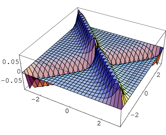
Figure 9: Flat 5D Massless Scalar Propagator ($Z_{2}$-odd, Dirichlet-Dirichlet b.c.), ${\tilde{p}}$=3 >> 1/$l$ , space-like, S¹-boundary is not influenced, Sec.9.1(3S)

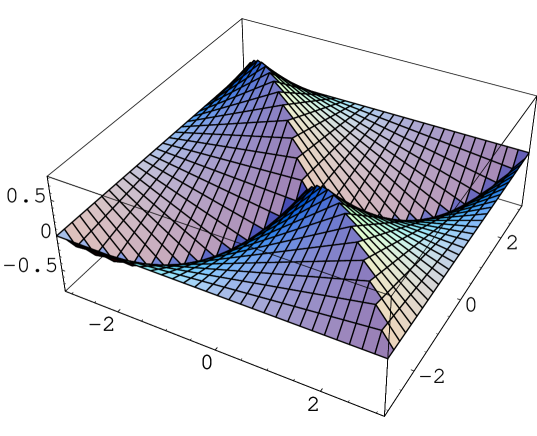
Figure 10: Flat 5D Massless Scalar Propagator ($Z_{2}$-odd, Dirichlet-Dirichlet b.c.), ${\hat{p}}$=0.03 << 1/$l$ , time-like, Sec.9.1(1T), S¹-boundary is strongly influenced

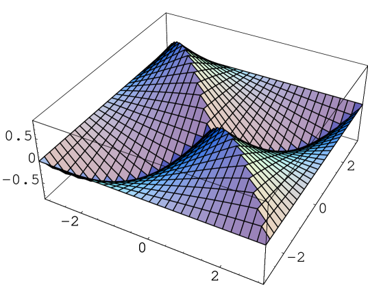
Figure 11: Flat 5D Massless Scalar Propagator ($Z_{2}$-odd, Dirichlet-Dirichlet b.c.), ${\hat{p}}$=0.3 $\sim$ 1/$l$ , time-like, Sec.9.1(2T)

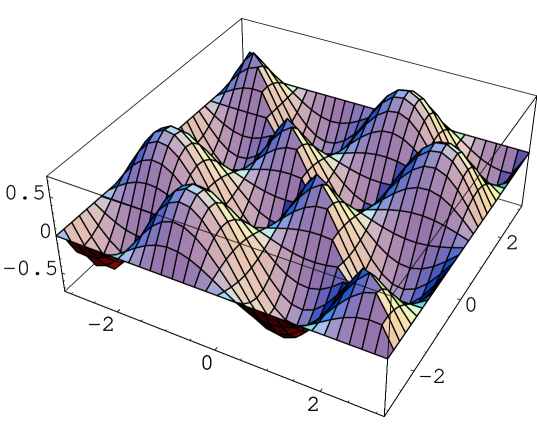
Figure 12: Flat 5D Massless Scalar Propagator ($Z_{2}$-odd, Dirichlet-Dirichlet b.c.), ${\hat{p}}$=1.7 > 1/$l$ , time-like, Sec.9.1(3T)

9.2 Warped 5D Scalar Propagator (Z₂-Odd, Dirichlet-Dirichlet b.c.)

We graphically show the P/M propagator behaviour of 5D scalar , with P=$-1$, in the warped geometry: (201) with (192) for $p^{2}>0$, (202) for $p^{2}<0$. Dirichlet b.c. is imposed on all fixed points $(y,y^{\prime}=0,\pm l)$. As for the choice of the value of $\omega$, we have the following possibilities: 1) $\omega\ll 1/l$,  2) $\omega<1/l$,  3) $\omega\sim 1/l$,  4) $\omega>1/l$,  5) $\omega\gg 1/l$.  Case 1) is important for approaching the flat limit from the warped geometry. Case 5) is the situation in the real world because we know Tev(Weak)-scale/Planck-scale =10^-16=$\exp(-\omega l)$. For simplicity, we take the case 4) for the display of graphs. The values are
$l$=$\pi$, 1/$l$$\sim$0.3, $\omega$=1, T=$\omega$ $\exp(-\omega l)$ $\sim$ 0.04
We use the following notation.
${\tilde{p}}\equiv\sqrt{p^{2}}$ for $p^{2}>0$(space-like); ${\hat{p}}\equiv\sqrt{-p^{2}}$ for $p^{2}<0$(time-like)

(A) Space-Like Case

For the y-coordinate presentation, we use the following propagator function.

$$G_{p}(y,y^{\prime})=K_{p}(Y(y,y^{\prime}),Y^{\prime}(y,y^{\prime})){\quad,}$$

$$K_{p}(Y,Y^{\prime})=\frac{1}{2\omega}\exp(2\omega|Y|+2\omega|Y^{\prime}|)\epsilon(Y)\epsilon(Y^{\prime})\times$$

$$\frac{\{{\bf I}_{0}(\frac{{\tilde{p}}}{\omega}){\bf K}_{0}(\frac{{\tilde{p}}}{\omega}\mbox{e}^{\omega|Y|})-{\bf K}_{0}(\frac{{\tilde{p}}}{\omega}){\bf I}_{0}(\frac{{\tilde{p}}}{\omega}\mbox{e}^{\omega|Y|})\}\{{\bf I}_{0}(\frac{{\tilde{p}}}{T}){\bf K}_{0}(\frac{{\tilde{p}}}{\omega}\mbox{e}^{\omega|Y^{\prime}|})-{\bf K}_{0}(\frac{{\tilde{p}}}{T}){\bf I}_{0}(\frac{{\tilde{p}}}{\omega}\mbox{e}^{\omega|Y^{\prime}|})\}}{{\bf I}_{0}(\frac{{\tilde{p}}}{T}){\bf K}_{0}(\frac{{\tilde{p}}}{\omega})-{\bf K}_{0}(\frac{{\tilde{p}}}{T}){\bf I}_{0}(\frac{{\tilde{p}}}{\omega})}{\quad,}$$ (210)

where $Y(y,y^{\prime})$ and $Y^{\prime}(y,y^{\prime})$ are defined in (70).

(1S) ${\tilde{p}}$ << 1/$l$ < $\omega$ , Fig.13
2 sharp up-ward spikes and 2 sharp down-ward spikes appear at corners. The effective thickness of the spikes is 1/$\omega$. (Note again that the top surface is cut at an appropriate height.) The size of the global upheaval and downheaval is $l$. The boundary constraint is dominant. This is the "boundary phase". There is a flat region around the center $(y=y^{\prime}=0)$. The propagator vanishes there. This means that the bulk propagation, near the Planck brane, gives no contribution to the amplitude. On the other hand, near the Tev brane $(y,y^{\prime}=\pm l)$, it gives a sizable effect.

We will see the warped scale parameter $\omega$ appears in all "phases".

(2S) 1/$l$ < ${\tilde{p}}$ $\sim$ $\omega$ , Fig.14
2 walls with sharp edges and 2 sharp valleys develop along the diagonal axes from the corners to the center. Their thickness is 1/${\tilde{p}}$ $\sim$ 1/$\omega$. The flat region near the center disappears. Absolute value of the effective height decreases.

(3S) 1/$l$ < $\omega$ < ${\tilde{p}}$ , Fig.15
Walls and valleys develop from the coners almost to the center. The effective thickness of them is 1/${\tilde{p}}$ near the corners and is 1/$\omega$ near the center. There is no boundary effect. This is the "dynamical phase". There is no flat region near the center, whereas in the off-diagonal region there appears the zero-value flat region. This means the bulk propagation takes place only for the case $y^{\prime}\pm y\sim 0$. Absolute value of the effective height decreases rapidly as ${\tilde{p}}$ increases.

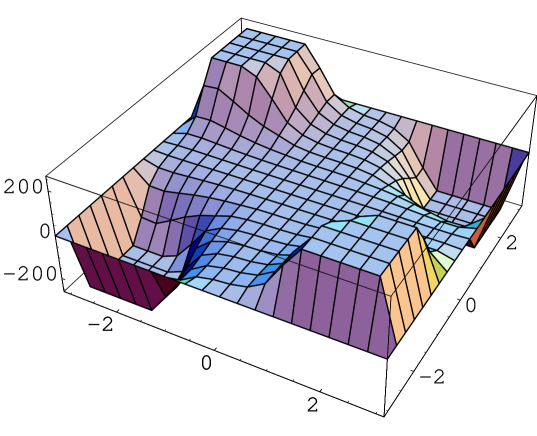
Figure 13: Warped 5D Scalar Propagator ($Z_{2}$-odd, Dirichlet-Dirichlet b.c.), ${\tilde{p}}$=0.005 << T < 1/$l$ <$\omega$, space-like, Sec.9.2(1S), "boundary phase"

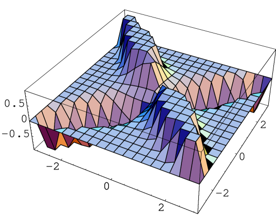
Figure 14: Warped 5D Scalar Propagator ($Z_{2}$-odd, Dirichlet-Dirichlet b.c.), T << 1/$l$ < ${\tilde{p}}$=1=$\omega$, space-like, Sec.9.2(2S)

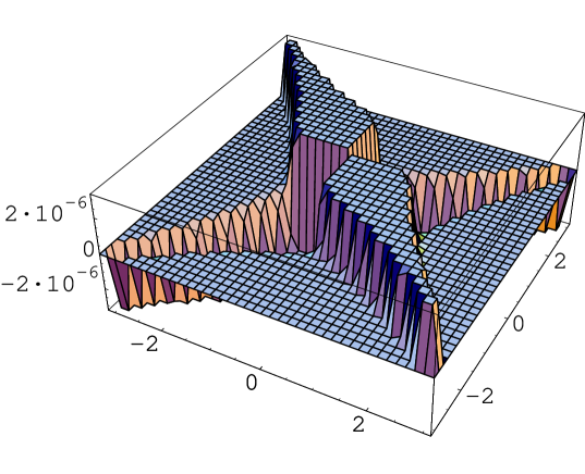
Figure 15: Warped 5D Scalar Propagator ($Z_{2}$-odd, Dirichlet-Dirichlet b.c.), T << 1/$l$ < $\omega$ < ${\tilde{p}}$=5, space-like, Sec.9.2(3S)

(B) Time-Like Case

For the y-coordinate presentation, we use the following propagator function.

$$G_{p}(y,y^{\prime})=K_{p}(Y(y,y^{\prime}),Y^{\prime}(y,y^{\prime})){\quad,}$$

$$K_{p}(Y,Y^{\prime})=\frac{1}{2\omega}\exp(2\omega|Y|+2\omega|Y^{\prime}|)\epsilon(Y)\epsilon(Y^{\prime})\times$$

$$\frac{\{{\bf J}_{0}(\frac{{\hat{p}}}{\omega}){\bf N}_{0}(\frac{{\hat{p}}}{\omega}\mbox{e}^{\omega|Y|})-{\bf N}_{0}(\frac{{\hat{p}}}{\omega}){\bf J}_{0}(\frac{{\hat{p}}}{\omega}\mbox{e}^{\omega|Y|})\}\{{\bf J}_{0}(\frac{{\hat{p}}}{T}){\bf N}_{0}(\frac{{\hat{p}}}{\omega}\mbox{e}^{\omega|Y^{\prime}|})-{\bf N}_{0}(\frac{{\hat{p}}}{T}){\bf J}_{0}(\frac{{\hat{p}}}{\omega}\mbox{e}^{\omega|Y^{\prime}|})\}}{{\bf J}_{0}(\frac{{\hat{p}}}{T}){\bf N}_{0}(\frac{{\hat{p}}}{\omega})-{\bf N}_{0}(\frac{{\hat{p}}}{T}){\bf J}_{0}(\frac{{\hat{p}}}{\omega})}{\quad,}$$ (211)

where $Y(y,y^{\prime})$ and $Y^{\prime}(y,y^{\prime})$ are defined in (70).

(1T) ${\hat{p}}$ << 1/$l$ < $\omega$ , Fig.16
The behaviour is quite similar to the space-like case (1S) above. The fact that, for low 4D momentum (${\hat{p}}$), the P/M propagator behaviours of the space-like case and of the time-like case are similar, is widely valid. See other cases below.

(2T) 1/$l$ < ${\hat{p}}$ $\sim$ $\omega$ , Fig.17
Wavy behaviour appears. Sharp spikes gather near the 4 corners and form groups within the range of order $1/\omega=1/{\hat{p}}$. Two types of waves are there. One type has the small wave-length of order 1/${\hat{p}}$=1/$\omega$, and the waves of this type appear along the 4 rims. The other type has the long wave-length of order $l$, which comes from the boundary constraint. It appears in the center and forms a very moderate hill. The propagator takes nearly 0 value there. This is contrasting with the space-like case. As the whole configuration, $Z_{2}$ oddness disappears.

(3T) 1/$l$ < $\omega$ < ${\hat{p}}$ , Fig.18
Spikes and two types of waves are there. It is roughly similar to (2T). The plain in the center forms clearly a disk. The propagator takes nearly 0 value there. This is contrasting with the space-like case. The overall height decreases. As in (2T), $Z_{2}$ oddness disappears. Although the scale $l$ looks to appear as the radius of the plain around the center, the main configuration is free from the boundary effect. It is nearly the "dynamical phase".

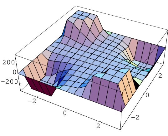
Figure 16: Warped 5D Scalar Propagator ($Z_{2}$-odd, Dirichlet-Dirichlet b.c.), ${\hat{p}}$=0.005 << T < 1/$l$ <$\omega$, time-like, Sec.9.2(1T)

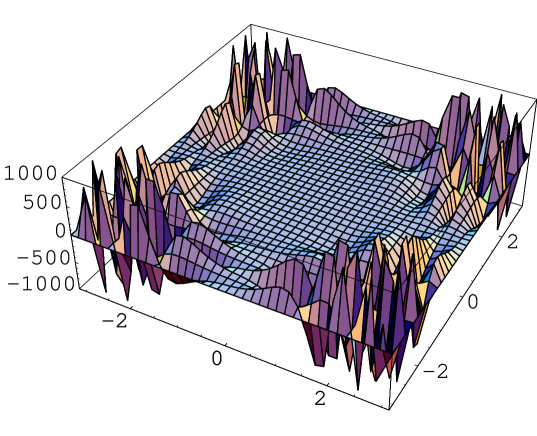
Figure 17: Warped 5D Scalar Propagator ($Z_{2}$-odd, Dirichlet-Dirichlet b.c.), T << 1/$l$ < ${\hat{p}}$=1=$\omega$, time-like, Sec.9.2(2T)

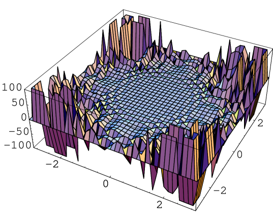
Figure 18: Warped 5D Scalar Propagator ($Z_{2}$-odd, Dirichlet-Dirichlet b.c.), T << 1/$l$ < $\omega$ < ${\hat{p}}$=5, time-like, Sec.9.2(3T)

From (1S) to (3S), from (1T) to (3T), the ratio $\omega/p$ decreases. We cannot take the flat limit in this way. In fact the scale $\omega$ remains in all "phases". The correct condition for the flat limit is both $\omega\ll 1/l$ and $\omega\ll p$ are satisfied. We have confirmed that, taking the values $l=\pi,\ \omega=0.001\ (\omega\ll 1/l)$, the warped propagators (210) and (211) produce graphs quite similar to the flat results of Sec.9.1 (Fig.7-12).

10 Solving $\delta(0)$-problem and the deformation of propagator

P/M propagator for 5D scalar is, for the space-like 4 momentum case, given by (58). It is expressed as

$$G_{p}(y,y^{\prime})=\frac{1}{4{\tilde{p}}\sinh{\tilde{p}}l}\left[\{\cosh 2{\tilde{p}}v_{+}(y,y^{\prime})-\cosh 2{\tilde{p}}v_{-}(y,y^{\prime})\}\cosh{\tilde{p}}l\right.$$

$$\left.+\{-\sinh 2{\tilde{p}}v_{+}(y,y^{\prime})+\sinh 2{\tilde{p}}v_{-}(y,y^{\prime})\}\sinh{\tilde{p}}l\right]{\quad.}$$ (212)

where $v_{-}$ and $v_{+}$ are defined by

$$v_{\mp}(y,y^{\prime})\equiv{\frac{1}{2}}|y^{\prime}\mp y|\quad:\quad y\ \leftrightarrow\ y^{\prime}\ \ \mbox{symmetric}{\quad.}$$ (213)

Using the following relations:

$$\frac{\partial v_{-}}{\partial y}=-{\frac{1}{2}}\epsilon(y^{\prime}-y){\quad,}\quad\frac{\partial v_{-}}{\partial y^{\prime}}={\frac{1}{2}}\epsilon(y^{\prime}-y)$$

$$\frac{\partial v_{+}}{\partial y}={\frac{1}{2}}\epsilon(y^{\prime}+y){\quad,}\quad\frac{\partial v_{+}}{\partial y^{\prime}}={\frac{1}{2}}\epsilon(y^{\prime}+y)$$

$$\frac{\partial^{2}v_{-}}{\partial y^{2}}=\delta(y^{\prime}-y){\quad,}\quad\frac{\partial^{2}v_{-}}{\partial y^{\prime}\partial y}=-\delta(y^{\prime}-y){\quad,}\quad\frac{\partial^{2}v_{-}}{\partial{y^{\prime}}^{2}}=\delta(y^{\prime}-y)$$

$$\frac{\partial^{2}v_{+}}{\partial y^{2}}=\delta(y^{\prime}+y){\quad,}\quad\frac{\partial^{2}v_{+}}{\partial y^{\prime}\partial y}=\delta(y^{\prime}+y){\quad,}\quad\frac{\partial^{2}v_{+}}{\partial{y^{\prime}}^{2}}=\delta(y^{\prime}+y)$$ (214)

we obtain, for the flat case (212),

$$\left.\frac{\partial^{2}G_{p}}{\partial y\partial y^{\prime}}\right|_{y=y^{\prime}=0}=-\delta(0)+{\frac{1}{2}}{\tilde{p}}\coth{\tilde{p}}l{\quad,}$$

$$\left.\frac{\partial^{2}G_{p}}{\partial y\partial y^{\prime}}\right|_{y=0,y^{\prime}=\pm l}={\frac{1}{2}}\frac{{\tilde{p}}}{\sinh{\tilde{p}}l}{\quad,}$$

$$\left.\frac{\partial^{2}G_{p}}{\partial y\partial y^{\prime}}\right|_{y=y^{\prime}=\pm l}=-\delta(0)+{\frac{1}{2}}{\tilde{p}}\coth{\tilde{p}}l{\quad.}$$ (215)

The above result says the bulk scalar propagation starting and ending at the Planck brane and that starting and ending at Tev brane are the same. The propagation starting at the Planck(Tev) brane and ending at the Tev(Planck) brane does not have $\delta(0)$ singularity.

The $\delta(0)$ problem first appeared in the analysis of 11D supergravity on a manifold with boundary in relation to the $E_{8}\times E_{8}$ heterotic string and M-theory[11]. It was shown, using a simpler model, that the problem generally occurs in the bulk-boundary theory[22]. When the bulk scalar $\Phi$ has a derivative ($\partial_{y}$) coupling with other field (this is the case of Mirabelli-Peskin model), the $\Phi$ propagator part in a quantum-loop amplitude appears as the form $\partial^{2}G_{p}/\partial y\partial y^{\prime}$. In Ref.[22], the cancellation of $\delta(0)$ was shown in a self energy calculation using KK-expansion. The cancellation was further confirmed in an improved way in Ref.[23, 24]. The first equation in (215) exactly coincides with the results in these papers. In the papers, however, the equation was obtained by summing all KK-modes contribution. In this paper the same equation is obtained without doing the KK-summation.

For the warped case, the corresponding propagator (5D scalar, space-like 4 momentum, Dirichlet b.c.) is given in (201). After calculation using (214), we obtain

$$\left.\frac{\partial^{2}G_{p}}{\partial y\partial y^{\prime}}\right|_{y=y^{\prime}=0}=-\delta(0)-2\omega+{\tilde{p}}\frac{{\bf I}_{0}(\frac{{\tilde{p}}}{T}){\bf K}_{1}(\frac{{\tilde{p}}}{\omega})+{\bf K}_{0}(\frac{{\tilde{p}}}{T}){\bf I}_{1}(\frac{{\tilde{p}}}{\omega})}{I_{0}(\frac{{\tilde{p}}}{T}){\bf K}_{0}(\frac{{\tilde{p}}}{\omega})-{\bf K}_{0}(\frac{{\tilde{p}}}{T}){\bf I}_{0}(\frac{{\tilde{p}}}{\omega})}{\quad.}$$ (216)

We confirm eq.(216) leads to the first equation of eq.(215) in the limit: $\omega/{\tilde{p}}\rightarrow+0,\ {\tilde{p}}l=$fixed. This shows the warped case is , at the propagator level, continuously connected with the flat one. The result (216) says that the warped version of the Mirabelli-Peskin model does not suffer from the $\delta(0)$ problem.

In Ref.[23], it is shown that the finite part of above expressions , (215) and (216), can be regarded as a "deformation" factor from the ordinary 4D theory propagator. The linear divergence, for ${\tilde{p}}\rightarrow\infty$, of the finite part just gives the UV-divergence due to 5D quantum fluctuation. Both flat and warped cases are non-renormalizable in this sense. See Sec.11 for further discussion about the renormalizability.

11 Discussions and Conclusion

We have treated QFT in the 5D flat and warped space-time. The Z₂-parity is respected. The P/M propagator is closely analyzed. Its singular properties are systematically treated by the use of the absolute functions. We have obtained the visual output of various P/M propagators, which enables us to know the various "phases" depending upon the choice of fields (scalar, vector, $\cdots$), boundary conditions (Dirichlet, Neumann), space-time geometry (flat, warped), the 4D momentum property(space-like, time-like) and its magnitude ($\sqrt{|p^{2}|}$ in relation to $1/l$ and $\omega$). It is shown that the eigen-mode expansion approach is equivalent to the P/M propagator approach. They are related by the Fourier-expansion for the flat case and by the Strum-Liouville expansion for the warped case. The Dirac’s bra and ket vector formalism is naturally introduced for quantizing the 5D (flat and warped) space-time with Z₂-parity.

We add some comments and discussions as follows.

1) The Feynman rule for the present approach is straightforward and is given in Ref.[9]. The characteristic points are the appearance of the metric factors at vertices and the extra-axis integral form restricted by the directedness of the extra coordinate.

2) BRS structure is important for defining physical quantities in gauge theories. It is very successful in the 4D renormalizable theories. For the present model of higher dimensions, the structure is missing. The formal higher dimensional extension is possible, but the treatment of the extra dimension part is quite obscure. In Ref.[9], some Ward identities seem to work.

3) Generally the string theory is regarded advantageous over the QFT because the fundamental unit of the string tension $\alpha^{\prime}$ are there and the extendedness "softens" the singularities. The present approach is based on the higher-dimensional QFT. The extendedness parameter appears as the thickness $\omega$. The situation of the boundary conditions and the "brane" formation looks similar to that in the string theory. In particular, the role of the extra-axis looks to correspond to that of the open string which is used to define the D-brane. Of course, these similarities come from the fact that the original models are invented and examined, triggered by the string theory development. We point out the present approach could reveal some important regularization aspect of the string theory in a simplified way. In this respect, it is worth discussing the regularization in the present approach. In Fig.19, the integration space is shown. The horizontal axis is z-coordinate, and the range is $1/\omega\leq z\leq 1/T$. The vertical one is (the absolute value of) the 4D momentum. It runs in the range $\mu$($\equiv(T/\omega)\cdot\Lambda$, infrared cutoff)$\leq p\leq\Lambda$(ultraviolet cutoff). What region of (z,p)-space, shown in Fig.19, should be integrated is the present discussion point. Ref.[9] proposed the region:

$$p\ z\leq\frac{\Lambda}{\omega}{\quad,}\quad\frac{1}{\omega}\leq z\leq\frac{1}{T}{\quad,}$$ (217)

based on the concrete behaviour of the P/M propagator. (See Fig.40 and Fig.41 and their explanation in App.C.5.) Adapting the region (217), the $\beta$-function of the gauge coupling was finitely obtained[9]. Clearly this procedure is still primitive and some persuasive explanation is required. We propose here a new definition of the integral region. For the explanation we look the integral region in the space of (z-coordinate, 4D coordinate $x^{a}$), that is, the 5D coordinate space. See Fig.20. This is an equivalent description. For simplicity we take 5D Euclidean space. On the Planck-brane ($z=1/\omega$), the 4D space integral region is taken to be $1/\Lambda\leq x\equiv\sqrt{x^{a}x^{a}}\leq 1/\mu$. This region is 4 dimensional and forms the thick sphere-shell bounded by two $S^{3}$’s: one ($S^{3}_{\mbox{UV,Pla}}$) has the radius $1/\Lambda$ and the other ($S^{3}_{\mbox{IR,Pla}}$) has the radius $1/\mu$. On the Tev-brane ($z=1/T$), the 4D space integral region is $(1-\varepsilon)/\mu\leq x\leq 1/\mu$, where $\varepsilon$ is a new regularization parameter which tends to the positive 0, $\varepsilon\rightarrow+0$. As on the Planck-brane, the integral region is 4 dimensional and forms the thin sphere-shell bounded by two $S^{3}$’s: one ($S^{3}_{\mbox{UV,Tev}}$) has the radius $(1-\varepsilon)/\mu$ and the other ($S^{3}_{\mbox{IR,Tev}}$) has the radius $1/\mu$. Between the two branes ($1/\omega<z<1/T$), the integral region is the 5D volume bounded by two 4D regularization surfaces, $B_{UV}$ and $B_{IR}$, which can be determined by the minimal area principle and the boundary condition ($S^{3}_{UV,Pla}$ at $z=1/\omega$,$S^{3}_{UV,Tev}$ at $z=1/T$ for $B_{UV}$; $S^{3}_{IR,Pla}$ at $z=1/\omega$,$S^{3}_{IR,Tev}$ at $z=1/T$ for $B_{IR}$). Two regularization $S^{3}$ spheres, the UV sphere and the IR sphere, "flow" along the z-axis changing their radii: $B_{UV}$ describes the change of the UV sphere and $B_{IR}$ describes the change of the IR sphere. The advantage of the new definition is that, only at the fixed points, the artificial cutoffs are introduced. This is the same situation as taken in the ordinary 4D renormalizable theories. Between the fixed points, the regularization surfaces ($B_{UV},B_{IR}$) are not introduced by hand but determined by the bulk geometrical dynamics. If we view this new integral region in the (z,p)-space, the similar region to (217) is expected to be obtained. It is quite interesting that the regularization surfaces, $B_{UV}$ and $B_{IR}$, have similarity to the tree propagation of the closed string. The necessity of restriction on the integral region (217) strongly suggests the requirement of a new type "quantization". The integral region condition (217) looks a sort of the uncertainty relation. If this view is right, it is quite notable that the conjugate variable (in the quantum phase space) of the extra coordinate z is played by the absolute value of the 4D momentum, $\sqrt{|p^{2}|}$. The present standpoint described above is that the new relation comes from the minimal area principle. Hence the behaviour of the boundary surfaces, $B_{UV}$ and $B_{IR}$, plays an important role.

4) The flat system is characterized by the cyclic functions, while the warped one is characterized by the Bessel functions. Although the periodicity is lost in the latter system, both sets of functions constitute the complete orthonormal system and sufficiently deserve describing the quantum Hilbert space. The present analysis strongly suggests the Bessel function system can be regarded as a one-parameter deformed system of the cyclic functions.

5) As for the phenomenology application, besides the ones mentioned in the introduction, Higgs sector analysis based on 5D model is active. The Higgs field is identified with the extra-component of the bulk gauge field and the effective action is calculated under the name of "holographic pseudo-Goldstone boson"[26, 27, 28]. The form factors there correspond to P/M propagators $G_{p}(y,y^{\prime})$ of the present work.

Figure 19: Space of (z,p) for the integration. $\Lambda/\omega u$ is the position-dependent cutoff[9].

Figure 20: Space of (z,$x^{a}$) for the integration. $B_{IR}$, $S^{3}_{IR,Pla}$ and $S^{3}_{IR,Tev}$ can be similarly shown.

12 App. A : Sturm-Liouville expansion formula

We apply the Strum-Liouville expansion formula (203) to the flat case of Sec.2 and Sec.4.

$$\partial_{M}\partial^{M}\Phi(X)=-J(X){\quad,}$$

$$\Phi(X)={\int\frac{d^{4}p}{(2\pi)^{4}}}{\rm e}^{ipx}\Phi_{p}(y){\quad,}\quad J(X)={\int\frac{d^{4}p}{(2\pi)^{4}}}{\rm e}^{ipx}J_{p}(y){\quad,}$$

$$(-p^{2}+\frac{\partial^{2}}{\partial y^{2}})\Phi_{p}(y)=-J_{p}(y){\quad.}$$ (218)

Hence the general operator ${\hat{L}}$ (204) and the boundary points are given by

$$p(y)=1{\quad,}\quad q(y)=0{\quad,}\quad r(y)=1{\quad,}\quad\lambda=-p^{2}{\quad,}$$

$$a=0{\quad,}\quad b=l{\quad.}$$ (219)

We consider the odd Z₂-parity, P=$-1$, as in the text. Time-like case, $p^{2}<0$, is taken. The homogeneous equation and its "intermediate" solutions are given as

$$(\lambda+\frac{\partial^{2}}{\partial y^{2}})\psi(y)=0{\quad,}\quad-l\leq y\leq l$$

$$\varphi(y,\lambda)=(1/\sqrt{\lambda})\sin\sqrt{\lambda}y\quad\mbox{Dirichlet b.c. is satisfied at}\ y=0$$

$$\chi(y,\lambda)=(1/\sqrt{\lambda})\sin\sqrt{\lambda}(l-y)\quad\mbox{Dirichlet b.c. is satisfied at}\ y=l$$

(220)

The quantity $\Omega$, its zeros $\lambda_{n}$ and others are obtained as

$$\Omega(\lambda)=p(\varphi\chi^{\prime}-\chi\varphi^{\prime})=-(1/\sqrt{\lambda})\sin(\sqrt{\lambda}l){\quad,}$$

$$\Omega(\lambda_{n})=0{\quad,}\quad\lambda_{n}=(\frac{\pi}{l})^{2}n^{2},\ n=1,2,\cdots\ ,$$

$$\Omega^{\prime}(\lambda_{n})=-(l^{3}/2\pi^{2}n^{2})(-1)^{n}{\quad,}\quad k_{n}=\chi(y,\lambda_{n})/\varphi(y,\lambda_{n})=(-1)^{n+1}.$$ (221)

Using the above results and the eigen function $\psi_{n}(y)=\varphi(y,\lambda_{n})=(l/\pi n)\sin(\pi ny/l)$ , the Strum-Liouville expansion formula (203) reduces to

$$f(y)=\frac{2}{l}\sum_{n}(\sin\frac{n\pi y}{l})\int_{0}^{l}f(\xi)\sin(\frac{\pi n\xi}{l})d\xi{\quad.}$$ (222)

This is the familiar Fourier expansion formula for the odd function $f(y)$. Its Z₂ parity even version is used in (80) and the equivalence of the expansion approach and P/M approach is shown for the flat case.

13 App. B : General treatment of the propagator

In this appendix, we treat the propagator of AdS₅ space-time (Sec.6 and Sec.7) in the general way valid for the wide-range dynamics, that is, the Strum-Liuoville differential operator. The field equation (99) can be expressed, using 4D-Fourier transformed field $\Phi_{p}(z),J_{p}(z)$ defined in (218), as

$$\left\{\frac{d}{dz}p(z)\frac{d}{dz}-q(z)\right\}\Phi_{p}-p^{2}r(z)\Phi_{p}\equiv{\hat{L}}\Phi_{p}-p^{2}r(z)\Phi_{p}=-\frac{J_{p}(z)}{(\omega z)^{5}}\ ,$$

$$p(z)=\frac{1}{(\omega z)^{3}}{\quad,}\quad q(z)=\frac{m^{2}}{(\omega z)^{5}}{\quad,}\quad r(z)=\frac{1}{(\omega z)^{3}}{\quad.}$$ (223)

This is the Strum-Liouville differential equation with source term (the inhomogeneous case). We consider $p^{2}<0$ case (time-like). ($p^{2}>0$ case is similarly treated.) Z₂ parity is taken to be odd, P=$-1$, and the Dirichlet b.c. is taken both at $z=1/\omega$ and at $z=1/T$. (P=+1 case is similarly treated.)

(i) Homogeneous Solution ($J_{p}=0$)

$${\hat{L}}\Phi_{p}-p^{2}r(z)\Phi_{p}=0{\quad.}$$ (224)

This is the eigenvalue equation for the operator $r(z)^{-1}{\hat{L}}$. Two independent solutions are given by

$$(\omega z)^{2}\tilde{\bf J}_{\nu}(Mz){\quad,}\quad(\omega z)^{2}\tilde{\bf N}_{\nu}(Mz){\quad,}\quad M=\sqrt{-p^{2}}{\quad,}\quad\nu=\sqrt{4+\frac{m^{2}}{\omega^{2}}}{\quad.}$$ (225)

We introduce two "intermediate" solutions: $\varphi_{M}(z)$ which satisfies the b.c. only at $z=1/\omega$, and $\chi_{M}(z)$ which satisfies the b.c. only at $z=1/T$.

$$\varphi_{M}(z)=\frac{1}{N^{(1/\omega)}}(\omega z)^{2}(\tilde{\bf J}_{\nu}(Mz){\bf N}_{\nu}(\frac{M}{\omega})-\tilde{\bf N}_{\nu}(Mz){\bf J}_{\nu}(\frac{M}{\omega}))/{\bf N}_{\nu}(\frac{M}{\omega}){\quad,}$$

$$\chi_{M}(z)=\frac{1}{N^{(1/T)}}(\omega z)^{2}(\tilde{\bf J}_{\nu}(Mz){\bf N}_{\nu}(\frac{M}{T})-\tilde{\bf N}_{\nu}(Mz){\bf J}_{\nu}(\frac{M}{T}))/{\bf N}_{\nu}(\frac{M}{T}){\quad.}$$ (226)

The final solution is obtained by the requirement that $\varphi_{M}(z)$ and $\chi_{M}(z)$ become linearly-dependent each other.

$$\mbox{Wronskian}\quad W[\varphi_{M},\chi_{M}]\equiv\varphi_{M}\frac{d}{dz}\chi_{M}-\chi_{M}\frac{d}{dz}{\varphi_{M}}\propto\left\{{\bf J}_{\nu}(\frac{M}{\omega}){\bf N}_{\nu}(\frac{M}{T})-{\bf J}_{\nu}(\frac{M}{T}){\bf N}_{\nu}(\frac{M}{\omega})\right\}=0{\quad.}$$ (227)

This is because the solution must satisfy the Dirichlet b.c. at both points. The condition (227) fixes the set of eigenvalues $\{M_{n}\}$. The eigen function $\psi_{n}(z)$ is obtained as

$$\psi_{n}(z)=\varphi_{M}(z)|_{M=M_{n}}=\frac{1}{N^{(1/\omega)}_{n}}(\omega z)^{2}(\tilde{\bf J}_{\nu}(M_{n}z){\bf N}_{\nu}(\frac{M_{n}}{\omega})-\tilde{\bf N}_{\nu}(M_{n}z){\bf J}_{\nu}(\frac{M_{n}}{\omega}))/{\bf N}_{\nu}(\frac{M_{n}}{\omega})\ ,$$

$$=\chi_{M}(z)|_{M=M_{n}}{\quad,}$$

$$2\int_{\frac{1}{\omega}}^{\frac{1}{T}}r(z)\psi_{n}(z)\psi_{m}(z)dz=\delta_{nm}{\quad.}$$ (228)

(ii) Solution of (223), Inhomogeneous solution
  (iia) Expansion form
First we obtain the solution in the expansion form using the homogeneous solutions $\{\psi_{n}\}$ obtained in (i).

$$\Phi_{p}(z)=\sum_{n=1}^{\infty}c_{n}(p)\psi_{n}(z){\quad,}\quad{\hat{L}}\psi_{n}=-{M_{n}}^{2}r(z)\psi_{n}{\quad.}$$ (229)

Putting (229) into (223), we obtain

$$\sum_{n=1}^{\infty}c_{n}(p)(-p^{2}-{M_{n}}^{2})r(z)\psi_{n}(z)=-\frac{J_{p}(z)}{(\omega z)^{5}}{\quad.}$$ (230)

From the orthogonality (228), we can read the coefficient.

$$c_{n}(p)=\frac{f_{n}}{p^{2}+{M_{n}}^{2}}{\quad,}\quad f_{n}=\int_{1/\omega}^{1/T}\psi_{n}(z)\frac{J_{p}(z)}{(\omega z)^{5}}dz{\quad.}$$ (231)

Hence we obtain the solution.

$$\Phi_{p}(z)=\sum_{n=1}^{\infty}\frac{f_{n}}{p^{2}+{M_{n}}^{2}}\psi_{n}(z){\quad.}$$ (232)

This result corresponds to (122) of Sec.6.
  (iib) Closed form
We can also obtain the solution in the closed form using the "intermediate" solutions $\varphi_{M}(z),\chi_{M}(z)$ (226). The solution $\Phi_{p}(z)$ of (223) can be obtained as

$$\Phi_{p}(z)=-\chi_{M}(z)\int_{1/\omega}^{z}\frac{\varphi_{M}(\xi)}{[\varphi_{M}(\xi),\chi_{M}(\xi)]}\frac{J_{p}(\xi)}{(\omega\xi)^{5}}d\xi-\varphi_{M}(z)\int_{z}^{1/T}\frac{\chi_{M}(\xi)}{[\varphi_{M}(\xi),\chi_{M}(\xi)]}\frac{J_{p}(\xi)}{(\omega\xi)^{5}}d\xi\ ,$$

$$\quad[\varphi_{M}(z),\chi_{M}(z)]\equiv p(z)(\varphi_{M}(z){\chi_{M}}^{\prime}(z)-{\varphi_{M}}^{\prime}(z)\chi_{M}(z)){\quad,}$$ (233)

where $p(z)$ appears in (223). Because of $(d/dz)[\varphi_{M}(z),\chi_{M}(z)]=0$, we can express (233) as

$$[\varphi_{M}(z),\chi_{M}(z)]\equiv\Omega(M){\quad,}$$

$$\Phi_{p}(z)=-\frac{\chi_{M}(z)}{\Omega(M)}\int_{1/\omega}^{z}\varphi_{M}(\xi)\frac{J_{p}(\xi)}{(\omega\xi)^{5}}d\xi-\frac{\varphi_{M}(z)}{\Omega(M)}\int_{z}^{1/T}\chi_{M}(\xi)\frac{J_{p}(\xi)}{(\omega\xi)^{5}}d\xi{\quad.}$$ (234)

Let us here introduce the P/M propagator

$$G_{p}(z,\xi)\equiv\left\{\begin{array}[]{cc}-\frac{\chi_{M}(z)\varphi_{M}(\xi)}{[\varphi_{M}(\xi),\chi_{M}(\xi)]}\ ,&\frac{1}{\omega}\leq\xi\leq z\leq\frac{1}{T}\ (\mbox{R${}_{2}$ of Fig.6})\\ -\frac{\varphi_{M}(z)\chi_{M}(\xi)}{[\varphi_{M}(\xi),\chi_{M}(\xi)]}\ ,&\frac{1}{\omega}\leq z\leq\xi\leq\frac{1}{T}\ (\mbox{R${}_{1}$ of Fig.6})\end{array}\right.$$ (237)

where $M=\sqrt{-p^{2}}$. For other regions of Fig.6, $G_{p}$ is defined following the $Z_{2}$-parity property as done in Sec.7. In terms of the above propagator, (234) can be written as

$$\Phi_{p}(z)=\int_{1/\omega}^{1/T}G_{p}(z,\xi)\frac{J_{p}(\xi)}{(\omega\xi)^{5}}d\xi{\quad.}$$ (238)

The propagator (237) is the same one that is introduced in (143) of the text. Note that $K_{p}(z,\xi)$ of (202) corresponds to the lower part of (237).

Taking into account the expression (232) and the relation:

$$\frac{J_{p}(\xi)}{(\omega\xi)^{5}}=\sum_{n=1}^{\infty}f_{n}\psi_{n}(\xi){\quad,}\quad f_{n}\ \mbox{is defined in (\ref{gen9})}{\quad,}$$ (239)

we can read off, from (238), the following relation between the P/M propagator and the eigen functions $\{\psi_{n}\}$.

$$G_{p}(z,\xi)=\sum_{n=1}^{\infty}\frac{1}{p^{2}+{M_{n}}^{2}}{\frac{1}{2}}\left(\psi_{n}(z)\psi_{n}(\xi)-\psi_{n}(z)\psi_{n}(-\xi)\right){\quad.}$$ (240)

This is the same as (122) of Sec.6.

14 App. C : Behaviour of Various P/M propagators

The values for $l$ (half period), $\omega$ (thickness) are taken as
$l$=$\pi$, 1/$l$$\sim$0.3, $\omega$=1, T=$\omega$ $\exp(-\omega l)$ $\sim$ 0.04
We note the following notation used in the text.
${\tilde{p}}\equiv\sqrt{p^{2}}$ for $p^{2}>0$(space-like); ${\hat{p}}\equiv\sqrt{-p^{2}}$ for $p^{2}<0$(time-like)

14.1 App. C.1 : Flat 5D Massless Scalar Propagator ( $Z_{2}$-parity Even, Neumann-Neumann b.c.)

The behaviour of 5D massless scalar propagator with Z₂-parity even (P=1) is shown in Fig.21-26. Neumann b.c. is imposed for all fixed points. The P/M propagator is given by

$$G_{p}(y,y^{\prime})={\bar{K}}_{p}(Y(y,y^{\prime}),Y^{\prime}(y,y^{\prime})){\quad,}$$

$${\bar{K}}_{p}(Y,Y^{\prime})=\left\{\begin{array}[]{ccc}-\frac{\cosh{\tilde{p}}Y\cosh{\tilde{p}}(Y^{\prime}-l)}{2{\tilde{p}}\sinh{\tilde{p}}l}&{\tilde{p}}=\sqrt{p^{2}}&\mbox{for}\ p^{2}>0\\ \frac{\cos{\hat{p}}Y\cos{\hat{p}}(Y^{\prime}-l)}{2{\hat{p}}\sin{\hat{p}}l}&{\hat{p}}=\sqrt{-p^{2}}&\mbox{for}\ p^{2}<0\end{array}\right.$$ (243)

where $Y(y,y^{\prime})$ and $Y^{\prime}(y,y^{\prime})$ are defined in (70).

In this case, the scale parameter is the periodicity parameter $l$ only. We can characterize the behaviours by the momentum ${\tilde{p}}$ or ${\hat{p}}$ in comparison with 1/$l$.

(A) Space-Like

(1S) ${\tilde{p}}$ << 1/$l$ , Fig.21
Upheaval and downheaval surfaces front each other at sharp edges which correspond to the singularities at $y\pm y^{\prime}=0$. The size of the slope is $l$. The boundary constraint is strong. This is the ’boundary phase’. The scale p does not appear in the graph.

(2S) ${\tilde{p}}$ $\sim$ 1/$l$ , Fig.22
The gross shape is similar to (1S). The height decreases.

(3S) ${\tilde{p}}$ >> 1/$l$ , Fig.23
Valleys run along the diagonal axes. The configuration is free from the boundary constraint. This is the ’dynamical phase’. The size of the valley-width is 1/${\tilde{p}}$. In the off-diagonal region ($y\pm y^{\prime}\neq 0$), flat planes appear and the propagator takes nearly 0 there. The height decreases furthermore.

(B) Time-Like

(1T) ${\hat{p}}$ << 1/$l$ , Fig.24
Shape and height are similar to the space-like case. This is the ’boundary phase’.

(2T) ${\hat{p}}$ $\sim$ 1/$l$ , Fig.25
The absolute value of the height increases and decreases. Shape is similar to the space-like case.

(3T) ${\hat{p}}$ >> 1/$l$ , Fig.26
The wavy behaviour appears. The singularity-lines are buried in the waves. Boundary constraint is not effective. This is the ’dynamical phase’. The size of the wave length is 1/${\hat{p}}$.

Compared with the space-like case, the height does not so much change for the time-like case.

Figure 21: Flat 5D Massless Scalar Propagator ( Z₂-parity even, Neumann-Neumann b.c.), ${\tilde{p}}$=0.03 << 1/$l$ , space-like, App.C.1(1S). "Boundary phase".

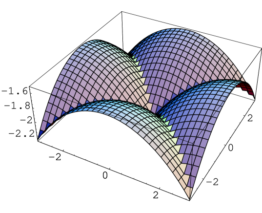
Figure 22: Flat 5D Massless Scalar Propagator ( Z₂-parity even, Neumann-Neumann b.c.), ${\tilde{p}}$=0.3 $\sim$ 1/$l$, space-like, App.C.1(2S)

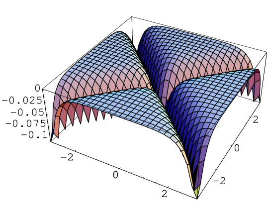
Figure 23: Flat 5D Massless Scalar Propagator ( Z₂-parity even, Neumann-Neumann b.c.), ${\tilde{p}}$=3 >> 1/$l$, space-like, App.C.1(3S). The "dynamical phase".

Figure 24: Flat 5D Massless Scalar Propagator ( Z₂-parity even, Neumann-Neumann b.c.), ${\hat{p}}$=0.03 << 1/$l$, time-like, App.C.1(1T). The "boundary phase".

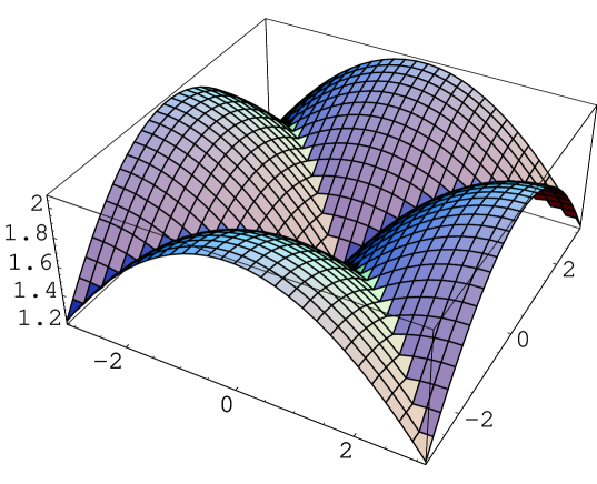
Figure 25: Flat 5D Massless Scalar Propagator ( Z₂-parity even, Neumann-Neumann b.c.), ${\hat{p}}$=0.3 $\sim$ 1/$l$, time-like, App.C.1(2T).

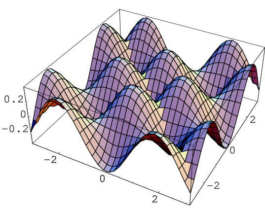
Figure 26: Flat 5D Massless Scalar Propagator ( Z₂-parity even, Neumann-Neumann b.c.), ${\hat{p}}$=1.7 >> 1/$l$, time-like, App.C.1(3T).

14.2 App. C.2 : Flat 5D Massless Scalar Propagator ($Z_{2}$-parity Odd, Dirichlet-Neumann b.c.)

The behaviour of 5D massless scalar flat propagators with the mixed b.c. are shown in Fig.27-32. $Z_{2}$-parity is taken to be odd: P=$-$1. Dirichlet b.c. is imposed for y=0, while Neumann b.c. for y=$\pm l$. The P/M propagator is given by

$$G_{p}(y,y^{\prime})={\bar{K}}_{p}(Y(y,y^{\prime}),Y^{\prime}(y,y^{\prime})){\quad,}$$

$${\bar{K}}_{p}(Y,Y^{\prime})=\left\{\begin{array}[]{ccc}-\frac{\sinh{\tilde{p}}Y\cosh{\tilde{p}}(Y^{\prime}-l)}{2{\tilde{p}}\cosh{\tilde{p}}l}&{\tilde{p}}=\sqrt{p^{2}}&\mbox{for}\ p^{2}>0\\ -\frac{\sin{\hat{p}}Y\cos{\hat{p}}(Y^{\prime}-l)}{2{\hat{p}}\cos{\hat{p}}l}&{\hat{p}}=\sqrt{-p^{2}}&\mbox{for}\ p^{2}<0\end{array}\right.$$ (246)

where $Y(y,y^{\prime})$ and $Y^{\prime}(y,y^{\prime})$ are defined in (70).

In this case, the scale parameter is the periodicity parameter $l$ only. We characterize the behaviours by the momentum ${\tilde{p}}$ or ${\hat{p}}$ in comparison with 1/$l$.

(A) Space-Like

(1S) ${\tilde{p}}$ << 1/$l$ , Fig.27
Slanted flat surfaces front each other along the diagonal lines ($y\pm y^{\prime}=0$, the singularities). The size of the surface is $l$. Boundary constraint is strong. This is the ’boundary phase’. The scale p does not appear in the graph.

(2S) ${\tilde{p}}$ $\sim$ 1/$l$ , Fig.28
The shape and the height are similar to (1S).

(3S) ${\tilde{p}}$ >> 1/$l$ , Fig.29
Walls and valleys run along the diagonal axes. The configuration is free from the boundary constraint. This is the ’dynamical phase’. The size of the wall (valley) thickness is 1/p. Absolute value of the effective height decreases.

(B) Time-Like

(1T) ${\hat{p}}$ << 1/$l$ , Fig.30
Shape and height are similar to the space-like case. This is the ’boundary phase’.

(2T) ${\hat{p}}$ $\sim$ 1/$l$  , Fig.31
The absolute value of the height increases and decreases by changing p within this region. The global shape does not change.

(3T) ${\hat{p}}$ >> 1/$l$ , Fig.32
The wavy behaviour appears. The singularity-lines are buried in the waves. Boundary constraint is not effective. This is the ’dynamical phase’. The size of the wave length is 1/${\hat{p}}$.

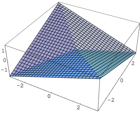
Figure 27: Flat 5D Massless Scalar Propagator ($Z_{2}$-parity Odd, Dirichlet-Neumann b.c.), ${\tilde{p}}$=0.03 << 1/$l$ , space-like, App.C.2(1S). The "boundary phase".

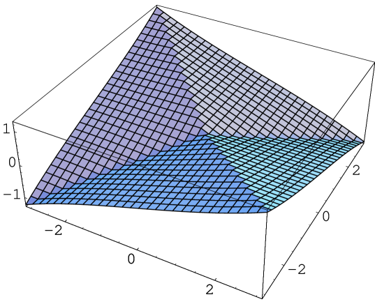
Figure 28: Flat 5D Massless Scalar Propagator ($Z_{2}$-parity Odd, Dirichlet-Neumann b.c.), ${\tilde{p}}$=0.3 $\sim$ 1/$l$, space-like, App.C.2(2S).

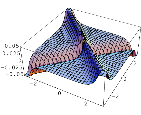
Figure 29: Flat 5D Massless Scalar Propagator ($Z_{2}$-parity Odd, Dirichlet-Neumann b.c.), ${\tilde{p}}$=3 >> 1/$l$, space-like, App.C.2(3S). The "dynamical phase".

Figure 30: Flat 5D Massless Scalar Propagator ($Z_{2}$-parity Odd, Dirichlet-Neumann b.c.), ${\hat{p}}$=0.03 << 1/$l$ , time-like, App.C.2(1T). The "boundary phase".

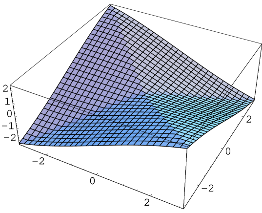
Figure 31: Flat 5D Massless Scalar Propagator ($Z_{2}$-parity Odd, Dirichlet-Neumann b.c.), ${\hat{p}}$=0.3 $\sim$ 1/$l$, time-like, App.C.2(2T).

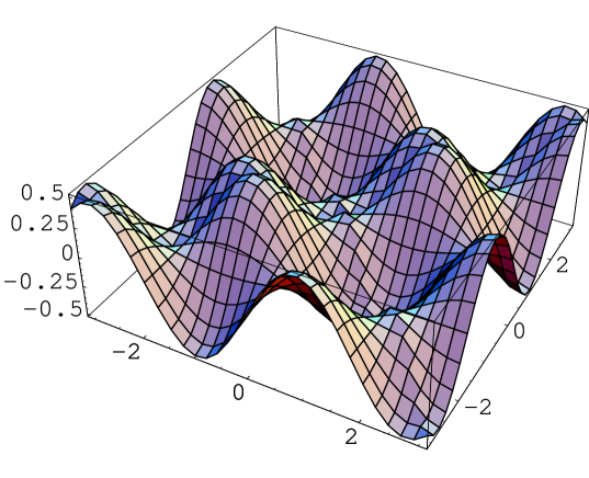
Figure 32: Flat 5D Massless Scalar Propagator ($Z_{2}$-parity Odd, Dirichlet-Neumann b.c.), ${\hat{p}}$=1.7 >> 1/$l$, time-like, App.C.2(3T). The "dynamical phase".

14.3 App. C.3 : z-Coordinate Representation and Warped 5D Scalar Propagator (Z₂-parity odd, Dirichlet-Dirichlet b.c., space-like 4-momentum)

We give here the P/M propagator behaviour in terms of z-coordinate. Its relation to y is given in (90). We take 5D scalar propagator with P=$-1$. Dirichlet b.c. is imposed on all fixed points. 4D momentum is space-like. The propagator function is given in (201) with (192). It can be reexpressed as follows using the ordinary Bessel functions and the sign function.

$$G_{p}(z,z^{\prime})=K_{p}(Z(z,z^{\prime}),Z^{\prime}(z,z^{\prime})){\quad,}$$

$$K_{p}(Z,Z^{\prime})=\frac{\omega^{3}}{2}Z^{2}{Z^{\prime}}^{2}\epsilon(Z)\epsilon(Z^{\prime})\times$$

$$\frac{\{{\bf I}_{0}(\frac{{\tilde{p}}}{\omega}){\bf K}_{0}({\tilde{p}}|Z|)-{\bf K}_{0}(\frac{{\tilde{p}}}{\omega}){\bf I}_{0}({\tilde{p}}|Z|)\}\{{\bf I}_{0}(\frac{{\tilde{p}}}{T}){\bf K}_{0}({\tilde{p}}|Z^{\prime}|)-{\bf K}_{0}(\frac{{\tilde{p}}}{T}){\bf I}_{0}({\tilde{p}}|Z^{\prime}|)\}}{{\bf I}_{0}(\frac{{\tilde{p}}}{T}){\bf K}_{0}(\frac{{\tilde{p}}}{\omega})-{\bf K}_{0}(\frac{{\tilde{p}}}{T}){\bf I}_{0}(\frac{{\tilde{p}}}{\omega})}{\quad,}$$ (247)

where $Z(z,z^{\prime})$ and $Z^{\prime}(z,z^{\prime})$ are defined in (201).

As we see the following graphs, large part of the whole image is naturally displayed. This means the z-coordinate is more suitable than y-coordinate for the warped geometry description. (Compare the height-region in Sec.9.2 (y-coordinate is used) and in this subsection for corresponding graphs.) From the z-coordinate property, however, it is hard to detect characteristic scales in the graphs.

The following graphs are re-drawing of those of Sec.9.2. They are displayed for ${\bar{R}}_{1}U{\bar{R}}_{2}$ region of the $(z,z^{\prime})$-plane (See Fig.6).

(1S) ${\tilde{p}}$ << 1/$l$ < $\omega$ , Fig.33

(2S) 1/$l$ < ${\tilde{p}}$ $\sim$ $\omega$ , Fig.34

(3S) 1/$l$ < $\omega$ < ${\tilde{p}}$ , Fig.35
If we go further larger ${\tilde{p}}$ ($1/l<\omega\ll{\tilde{p}}$), the situation is the "flat (z-)space limit" represented by eq.(6.16) of Ref.[9]. Compare with Fig.9.

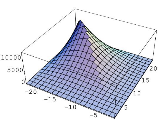
Figure 33: z-Coordinate Representation, Warped 5D Scalar Propagator (Z₂-parity odd, Dirichlet-Dirichlet b.c., ${\tilde{p}}$=0.005 << T < 1/$l$ <$\omega$, space-like, App.C.3(1S).

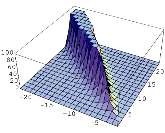
Figure 34: z-Coordinate Representation, Warped 5D Scalar Propagator (Z₂-parity odd, Dirichlet-Dirichlet b.c., T << 1/$l$ < ${\tilde{p}}$=1=$\omega$, space-like, App.C.3(2S).

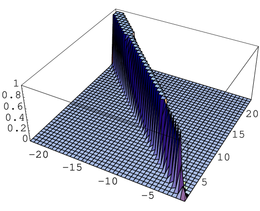
Figure 35: z-Coordinate Representation, Warped 5D Scalar Propagator (Z₂-parity odd, Dirichlet-Dirichlet b.c.), T << 1/$l$ < $\omega$ < ${\tilde{p}}$=5, space-like, App.C.3(3S).

14.4 App. C.4 : Warped 5D Massless Vector ($Z_{2}$-parity Even, Neumann-Neumann b.c., space-like 4 momentum)

In the warped case the theory has two scale parameters: thickness $\omega$ and the periodicity parameter $l$. The propagator behaviour is characterized by the relation between $\sqrt{|p^{2}|}$, $\omega$ and $1/l$.

In this subsection, the 5D vector propagator with $Z_{2}$-parity even (P=1) is examined. The Neumann b.c. is imposed on all fixed points. The P/M propagator is given by

$$G_{p}(y,y^{\prime})=K_{p}(Y(y,y^{\prime}),Y^{\prime}(y,y^{\prime})){\quad,}$$

$$K_{p}(Y,Y^{\prime})=\frac{1}{\omega}\exp(k|Y|+k|Y^{\prime}|)\times$$

$$\frac{\{{\bf I}_{0}(\frac{{\tilde{p}}}{\omega}){\bf K}_{1}(\frac{{\tilde{p}}}{\omega}\mbox{e}^{\omega|Y|})+{\bf K}_{0}(\frac{{\tilde{p}}}{\omega}){\bf I}_{1}(\frac{{\tilde{p}}}{\omega}\mbox{e}^{\omega|Y|})\}\{{\bf I}_{0}(\frac{{\tilde{p}}}{T}){\bf K}_{1}(\frac{{\tilde{p}}}{\omega}\mbox{e}^{\omega|Y^{\prime}|})+{\bf K}_{0}(\frac{{\tilde{p}}}{T}){\bf I}_{1}(\frac{{\tilde{p}}}{\omega}\mbox{e}^{\omega|Y^{\prime}|})\}}{{\bf I}_{0}(\frac{{\tilde{p}}}{\omega}){\bf K}_{0}(\frac{{\tilde{p}}}{T})-{\bf K}_{0}(\frac{{\tilde{p}}}{\omega}){\bf I}_{0}(\frac{{\tilde{p}}}{T})}{\quad,}$$ (248)

where $Y(y,y^{\prime})$ and $Y^{\prime}(y,y^{\prime})$ are defined in (70).

(1S) ${\tilde{p}}$ << 1/$l$ < $\omega$ , Fig.36
4 notches appear at 4 corners. The effective width of the notch is 1/$\omega$. The size of the global upheaval and downheaval is $l$. The boundary constraint is dominant. This is the "boundary phase". There is a flat region around the center $(y=y^{\prime}=0)$. The propagator takes a non-zero constant there. This means that the bulk propagation, near the Planck brane, simply gives a common constant , as the extra-space contribution, to the amplitude. On the other hand, near the Tev brane $(y,y^{\prime}=\pm l)$, it gives a "sizable" effect.

(2S) 1/$l$ < ${\tilde{p}}$ $\sim$ $\omega$ , Fig.37
4 valleys develop along the diagonal axes from the corners to the center. Their width is 1/${\tilde{p}}$ $\sim$ 1/$\omega$. The flat region near the center disappears. In the off-diagonal region ($y\pm y^{\prime}\neq 0$) , flat planes begin to appear and the propagator takes nearly 0 value there. The height decreases.

(3S) 1/$l$ < $\omega$ < ${\tilde{p}}$ , Fig.38
Valleys develop furthermore. The width of them is 1/${\tilde{p}}$ near the corners and is 1/$\omega$ near the center. There is no boundary effect. This is the "dynamical phase". There is no flat region near the center, whereas in the off-diagonal region there appears the flat region. The propagator value is 0 in this flat region. This means the bulk propagation takes place only for the case $y^{\prime}\pm y\sim 0$. Absolute value of the effective height decreases rapidly as ${\tilde{p}}$ increases. If we take further larger ${\tilde{p}}$ ($1/l<\omega\ll{\tilde{p}}$), the situation is the "flat limit". Compare with Fig.23.

Time-like case is given in App.C.6.

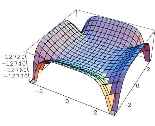
Figure 36: Warped 5D Massless Vector ($Z_{2}$-parity Even, Neumann-Neumann b.c.) ${\tilde{p}}$=0.005 << T$\sim$0.04 << 1/$l$$\sim$0.3 << $\omega$=1, space-like., App.C.4(1S)

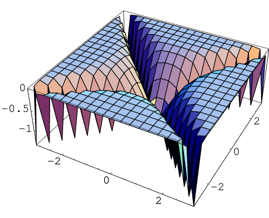
Figure 37: Warped 5D Massless Vector ($Z_{2}$-parity Even, Neumann-Neumann b.c.) T << 1/$l$ < ${\tilde{p}}$=1=$\omega$, space-like, App.C.4(2S)

Figure 38: Warped 5D Massless Vector ($Z_{2}$-parity Even, Neumann-Neumann b.c.), T << 1/$l$ < $\omega$ < ${\tilde{p}}$=5, space-like, App.C.4(3S).

14.5 App. C.5 : z-Coordinate Representation for Warped 5D Massless Vector ($Z_{2}$-parity Even, Neumann-Neumann b.c.,space-like)

We give here the P/M vector ($Z_{2}$-parity even, Neumann-Neumann b.c., space-like) propagator behaviour in terms of z-coordinate. The propagator expression is given in (248) using the y-coordinate. Here its z-coordinate expression is given.

$$G_{p}(z,z^{\prime})=K_{p}(Z(z,z^{\prime}),Z^{\prime}(z,z^{\prime})){\quad,}$$

$$K_{p}(Z,Z^{\prime})=\omega|Z||Z^{\prime}|\times$$

$$\frac{\{{\bf I}_{0}(\frac{{\tilde{p}}}{\omega}){\bf K}_{1}({\tilde{p}}|Z|)+{\bf K}_{0}(\frac{{\tilde{p}}}{\omega}){\bf I}_{1}({\tilde{p}}|Z|)\}\{{\bf I}_{0}(\frac{{\tilde{p}}}{T}){\bf K}_{1}({\tilde{p}}|Z^{\prime}|)+{\bf K}_{0}(\frac{{\tilde{p}}}{T}){\bf I}_{1}({\tilde{p}}|Z^{\prime}|)\}}{{\bf I}_{0}(\frac{{\tilde{p}}}{\omega}){\bf K}_{0}(\frac{{\tilde{p}}}{T})-{\bf K}_{0}(\frac{{\tilde{p}}}{\omega}){\bf I}_{0}(\frac{{\tilde{p}}}{T})}{\quad,}$$ (249)

where $Z(z,z^{\prime})$ and $Z^{\prime}(z,z^{\prime})$ are defined in (201).

The following graphs are re-drawing of those of App.C.4 using the z-coordinate. They are displayed for $R_{1}$U$R_{2}$ region of the $(z,z^{\prime})$-plane (See Fig.6).

(1S) ${\tilde{p}}$ << 1/$l$ < $\omega$ , Fig.39

(2S) 1/$l$ < ${\tilde{p}}$ $\sim$ $\omega$ , Fig.40

(3S) 1/$l$ < $\omega$ < ${\tilde{p}}$ , Fig.41
If we take further larger ${\tilde{p}}$, the configuration becomes the "flat (z-)space limit". Compare with Fig.23. ( The same situation has already appeared for the scalar propagator case, Fig.34 and Fig.35 in App.C.3. )

In the graphs of (2S) and (3S), we see, in their off-diagonal regions, the top surfaces very gradually approach the 0-value surface as they deviate from the diagonal axis: $G_{p}(z,z^{\prime})\sim-\exp(-{\tilde{p}}|z^{\prime}-z|)$. This is the "untrusted" region pointed out in ref.[9].

Figure 39: z-Coordinate Representation for Warped 5D Massless Vector ($Z_{2}$-parity Even, Neumann-Neumann b.c.), ${\tilde{p}}$=0.005 << T$\sim$0.04 << 1/$l$$\sim$0.3 << k=1, space-like, App.C.5(1S).

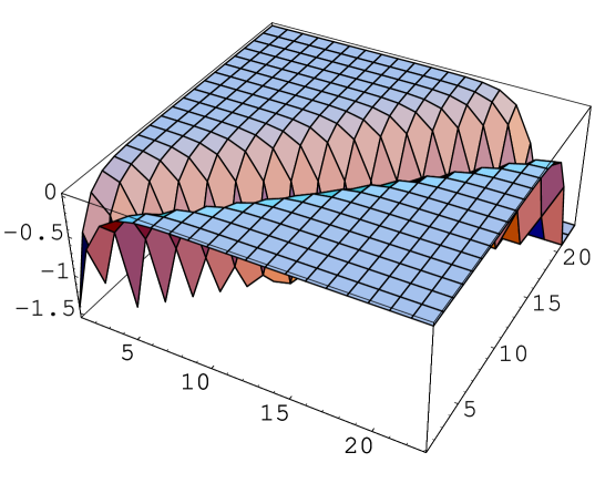
Figure 40: z-Coordinate Representation for Warped 5D Massless Vector ($Z_{2}$-parity Even, Neumann-Neumann b.c.), T << 1/$l$ < ${\tilde{p}}$=1=$\omega$, space-like, App.C.5(2S).

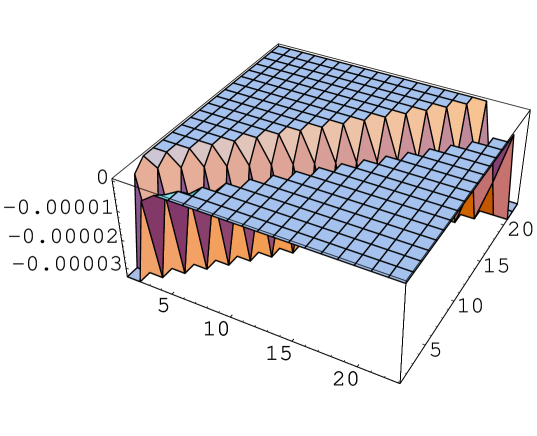
Figure 41: z-Coordinate Representation for Warped 5D Massless Vector ($Z_{2}$-parity Even, Neumann-Neumann b.c.), T << 1/$l$ < $\omega$ < ${\tilde{p}}$=5, space-like, App.C.5(3S)

14.6 App. C.6 : Warped 5D Massless Vector (Z₂-parity Even, Neumann-Neumann b.c., time-like 4 momentum)

Here we give the P/M propagator behaviour of the warped 5D massless vector (Z₂-parity Even, Neumann-Neumann b.c., time-like). The propagator is given by

$$G_{p}(y,y^{\prime})=K_{p}(Y(y,y^{\prime}),Y^{\prime}(y,y^{\prime})){\quad,}$$

$$K_{p}(Y,Y^{\prime})=-\frac{1}{\omega}\exp(k|Y|+k|Y^{\prime}|)\times$$

$$\frac{\{{\bf N}_{0}(\frac{{\hat{p}}}{\omega}){\bf J}_{1}(\frac{{\hat{p}}}{\omega}\mbox{e}^{\omega|Y|})-{\bf J}_{0}(\frac{{\hat{p}}}{\omega}){\bf N}_{1}(\frac{{\hat{p}}}{\omega}\mbox{e}^{\omega|Y|})\}\{{\bf N}_{0}(\frac{{\hat{p}}}{T}){\bf J}_{1}(\frac{{\hat{p}}}{\omega}\mbox{e}^{\omega|Y^{\prime}|})-{\bf J}_{0}(\frac{{\hat{p}}}{T}){\bf N}_{1}(\frac{{\hat{p}}}{\omega}\mbox{e}^{\omega|Y^{\prime}|})\}}{{\bf N}_{0}(\frac{{\hat{p}}}{\omega}){\bf J}_{0}(\frac{{\hat{p}}}{T})-{\bf J}_{0}(\frac{{\hat{p}}}{\omega}){\bf N}_{0}(\frac{{\hat{p}}}{T})}{\quad,}$$ (250)

where $Y(y,y^{\prime})$ and $Y^{\prime}(y,y^{\prime})$ are defined in (70).

This is the time-like case of App.C.4.

(1T) ${\hat{p}}$ << 1/$l$ < $\omega$ , Fig.42
The situation is quite similar to (1S) of App.C.4.

(2T) 1/$l$ < ${\hat{p}}$ $\sim$ $\omega$ , Fig.43
Wavy behaviour appears. Two types of waves are there. One type has the small wave-length of order 1/${\hat{p}}$=1/$\omega$, and the waves of this type gather near the 4 corners. The other type has the long wave-length of order $l$, which comes from the boundary constraint. In particular, there exists a very moderate hill around the center. The propagator takes nearly 0 value there. This is contrasting with the space-like case. The overall height decreases.

(3T) 1/$l$ < $\omega$ < ${\hat{p}}$ , Fig.44
Two types of waves are there. One type has the small wave-length of order 1/${\hat{p}}$, and the waves of this type gather near the 4 corners and the 4 rims. Their heights differ so much. The other type has the long wave-length of order $\omega$ and the very low height. These waves gather around the center and form a slightly wavy plain. The propagator takes nearly 0 value there. This is contrasting with the space-like case. The overall height decreases. Although the scale $l$ looks to appear as the radius of the plain around the center, the main configuration is free from the boundary effect. This is the "dynamical phase". When ${\hat{p}}$ becomes further larger, the configuration approaches a "flat limit". It differs from the flat result, Fig.26.

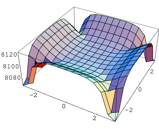
Figure 42: Warped 5D Massless Vector (Z₂-parity Even, Neumann-Neumann b.c.), ${\hat{p}}$=0.005 << T$\sim$0.04 << 1/$l$$\sim$0.3 << $\omega$=1, time-like. App.C.6(1T).

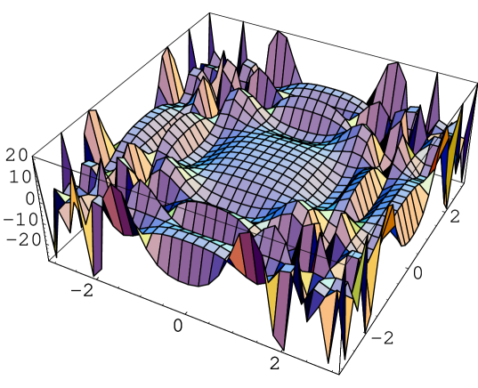
Figure 43: Warped 5D Massless Vector (Z₂-parity Even, Neumann-Neumann b.c.), T$\sim$0.04 << 1/$l$$\sim$0.3 < ${\hat{p}}$= $\omega$=1, time-like. App.C.6(2T).

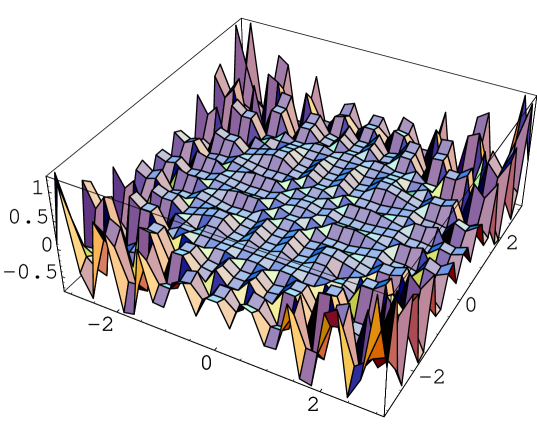
Figure 44: Warped 5D Massless Vector (Z₂-parity Even, Neumann-Neumann b.c.), T$\sim$0.04 << 1/$l$$\sim$0.3 < $\omega$=1 << ${\hat{p}}$=10, time-like. App.C.6(3T).

15 Acknowledgement

Parts of the content of this work have been already presented at YITP workshop on QFT and String (06.9.12, Kyoto, Japan), Joint Meeting of Pacific Region Particle Physics Communities (06.11.01,Hawaii,Honolulu,USA) and RIKEN Seminar(06.11.27, Wako, Japan). The authors thank N. Nakanishi, Hiroshi Suzuki and K. Oda for useful comments on the occasions.

References

- [1] L.Randall and R.Sundrum, Phys.Rev.Lett.83(1999)3370,hep-ph/9905221
- [2] L.Randall and R.Sundrum, Phys.Rev.Lett.83(1999)4690,hep-th/9906064
- [3] K. Agashe, G. Perez and A. Soni, Phys.Rev.D71(2005)016002, hep-ph/0408134
- [4] S.J. Brodsky and G.F.de Teramond, hep-th/0702205, "AdS/CFT and QCD"
- [5] J. Garriga and T. Tanaka, Phys.Rev.Lett.84(2000)2778, hep-th/9911055
- [6] S.B. Giddings, E. Katz and L. Randall, JHEP0003(2000)023, hep-th/0002091
- [7] A. Pomarol, Phys.Rev.Lett.85(2000)4004, hep-ph/0005293
- [8] T. Gherghetta and A. Pomarol, Nucl.Phys.B602(2001)3, hep-ph/0012378
- [9] L. Randall and M.D. Schwartz, JHEP 0111 (2001) 003, hep-th/0108114
- [10] E. Witten, Nucl.Phys.B471(1996)135, hep-th/9602070
- [11] P. Hořava and E. Witten, Nucl.Phys.B475(1996)94, hep-th/9603142
- [12] Th. Kaluza, Sitzungsberichte der K.Preussischen Akademite der Wissenschaften zu Berlin. p966 (1921)
- [13] O. Klein, Z. Physik 37 895 (1926)
- [14] P.A.M. Dirac, "The Principles of Quantum Mechanics", 4th Edition, Oxford Univ. Press, Oxford, 1958
- [15] D. V. Belyaev, hep-th/0509171, "Boundary conditions in the Mirabelli and Peskin model"
- [16] D. V. Belyaev, hep-th/0509172, "Boundary conditions in supergravity on a manifold with boundary"
- [17] S. Ichinose, Phys.Rev.D61(2000)055001
- [18] S. Ichinose and A. Murayama, Phys.Lett.B596 (2004) 123, hep-th/0405065
- [19] T. Gherghetta and A. Pomarol, Nucl.Phys.B586(2000)141, hep-ph/0003129
- [20] E.C. Titchmarsh, "Eigenfunction Expansions Associated with Second-order Differential Equations" (Part I), Second edition, Oxford University Press, Oxford, 1962.
- [21] S. Ichinose, Phys.Rev.D65(2002)084038, hep-th/0008245
- [22] E.A. Mirabelli and M.E. Peskin, Phys.Rev.D58(1998)065002, hep-th/9712214
- [23] S. Ichinose and A. Murayama, Nucl.Phys.B710(2005)255, hep-th/0401011
- [24] S. Ichinose and A. Murayama, Phys.Lett.B593(2004)242, hep-th/0403080
- [25] S. Ichinose and A. Murayama, hep-th/0606167, "The delta(0) Singularity in the Warped Mirabelli-Peskin Model"
- [26] K. Oda and A. Weiler, Phys.Lett.B606(2005)408, hep-ph/0410061
- [27] K. Agashe, R. Contino and A. Pomarol, Nucl.Phys.B719(2005)165, hep-ph/0412089
- [28] A. Falkowski, Phys.Rev.D75(2007)025017