Monte Carlo approach to nonperturbative strings
— demonstration in noncritical string theory

Abstract:

We show how Monte Carlo approach can be used to study the double scaling limit in matrix models. As an example, we study a solvable hermitian one-matrix model with the double-well potential, which has been identified recently as a dual description of noncritical string theory with worldsheet supersymmetry. This identification utilizes the nonperturbatively stable vacuum unlike its bosonic counterparts, and therefore it provides a complete constructive formulation of string theory. Our data with the matrix size ranging from $8$ to $512$ show a clear scaling behavior, which enables us to extract the double scaling limit accurately. The “specific heat” obtained in this way agrees nicely with the known result obtained by solving the Painleve-II equation with appropriate boundary conditions.

1 Introduction

Matrix models have been considered as one of the most powerful frameworks to formulate string theories in a nonperturbative manner. A fundamental viewpoint which links matrix models to string theories was given by ’t Hooft [1]. There Feynman diagrams which appear in matrix models are identified with discretized string worldsheets. However, if one takes the large-$N$ limit naively (the so-called planar limit), only the planar diagrams survive, which implies the appearance of a classical string theory. One way to formulate nonperturbative string theory using matrix models is therefore to look for a nontrivial large-$N$ limit, in which Feynman diagrams with all kinds of topology survive. The existence of such a limit has been first demonstrated in matrix models for noncritical string theory [5, 6, 7], and it is called the double scaling limit. (See also refs. [8, 9, 10, 11] for recent works, in which the double scaling limit appears in various contexts.)

It is generally believed that a similar idea can be applied also to critical string theories. The corresponding matrix models have been proposed in refs. [12, 13, 14], but the existence of a nontrivial large-$N$ limit is yet to be confirmed. To address such an issue, the 2d Eguchi-Kawai model [15] has been studied as a toy model. Indeed Monte Carlo simulation [16] demonstrated the existence of a one-parameter family of large-$N$ limits, which generalizes the Gross-Witten [17] planar large-$N$ limit. If one modifies the Eguchi-Kawai model by introducing the twist [18], the double scaling limit can be identified with the continuum limit of field theories on discrete non-commutative (NC) geometry [19]. The actual existence of such limits has been demonstrated by Monte Carlo simulations in the case of NC gauge theory in 2d [9] and 4d [11] and also in 3d NC scalar field theory [10]. In all these cases, it was observed that non-planar diagrams indeed affect the infrared dynamics drastically through the UV/IR mixing mechanism [20].

We consider that Monte Carlo simulation would be a powerful tool also to study matrix models for critical string theories. Technically the IIB matrix model [13] would be the least difficult among them since the space-time, on which the ten-dimensional ${\cal N}=1$ super Yang-Mills theory is defined, is totally reduced to a point. However, the integration over the fermionic matrices yields a complex Pfaffian, which makes the Monte Carlo simulation still very hard [21, 22]. An analogous model, which can be obtained by dimensionally reducing four-dimensional ${\cal N}=1$ super Yang-Mills theory to a point, does not have that problem, and Monte Carlo studies suggest the existence of a nontrivial large-$N$ limit [23].

The developments in the matrix description of critical string theories have also given a new perspective to noncritical string theory. For instance, in matrix quantum mechanics which describe $(1+1)$-dimensional string theory in the double scaling limit, the matrix degrees of freedom have been interpreted as the tachyonic open-string field living on unstable D0-branes [24, 25]. Based on this interpretation, matrix models with the double-well potential, which are known to be solvable, have been identified as a dual description of noncritical string theory with worldsheet supersymmetry [26, 27, 28]. An important property of these models is that they possess a stable nonperturbative vacuum unlike their bosonic counterparts, and therefore one can obtain a complete constructive formulation of string theory. It also provides us with a unique opportunity to test the validity and the feasibility of Monte Carlo methods for studying string theories nonperturbatively. In particular we are concerned with such questions as what kind of analysis is possible to extract the double scaling limit, and how large the matrix size should be.

In this work we consider the simplest model [29], namely a hermitian one-matrix model identified [28] as a dual of $\hat{c}=0$ noncritical string theory, which is sometimes referred to as the pure supergravity in the literature. We calculate correlation functions near the critical point, and investigate their scaling behavior to extract the double scaling limit. The results are then compared with a prediction obtained by a different approach. We hope that the lessons from this work would be useful in applying the same method to models which are not accessible by analytic methods.

The rest of this paper is organized as follows. In section 2 we introduce the one-matrix model, and present some simulation details. In section 3 we obtain explicit results in the planar limit, and compare them with the known analytical results. In section 4 we search for a double scaling limit by using only Monte Carlo data. The results are compared with the prediction obtained by the orthogonal-polynomial technique. In section 5 we present more detailed comparison with the analytical prediction. Section 6 is devoted to a summary and discussions. In the Appendix we briefly review the derivation of some asymptotic behaviors in the double scaling limit.

2 The model and some simulation details

The model we study in this paper is defined by

$$Z = \int d^{N^{2}}\!\!\phi\,\exp\left(-S\right)\ ,$$ (1)

$$S = \frac{N}{g}\,{\rm tr\,}\left(-\phi^{2}+\frac{1}{4}\phi^{4}\right)\ ,$$ (2)

where $\phi$ is an $N\times N$ hermitian matrix. We assume that the coupling constant $g$ is positive so that the action is bounded from below. Since the action takes the form of a double-well, the standard Metropolis algorithm using a trial configuration obtained by slightly modifying some components of the matrix would have a problem with ergodicity. In order to circumvent this problem, we perform the simulation as follows.

Let us diagonalize the hermitian matrix $\phi$ as $\phi=U\Lambda U^{-1}$, where $\Lambda={\rm diag}(\lambda_{1},\cdots,\lambda_{N})$ is a real diagonal matrix. Due to the SU($N$) invariance of the model, the angular variable $U$ can be integrated out. Thus we are left with a system of eigenvalues $\lambda_{i}$

$$Z = \int\prod_{i=1}^{N}d\lambda_{i}\,\exp(-\widetilde{S})\ ,$$ (3)

$$\widetilde{S} = \frac{N}{g}\sum_{i=1}^{N}\left(-\lambda_{i}^{2}+\frac{1}{4}\lambda_{i}^{4}\right)-\sum_{i<j}\log|\lambda_{i}-\lambda_{j}|^{2}\ ,$$ (4)

where the log term in eq. (4) comes from the Vandermonde determinant. Due to the $\lambda_{i}^{4}$ term in the action, the probability of $\lambda_{i}$ having a large absolute value is strongly suppressed. This can be seen also from the eigenvalue distribution in fig. 1, which actually has a compact support in the planar large-$N$ limit; see eqs. (6) and (7). We therefore restrict $|\lambda_{i}|$ to be less than some value $X$.

We first run a simulation with a reasonably large $X$. By measuring the eigenvalue distribution, we can obtain an estimate on $X$ that can be used without affecting the Monte Carlo results. We generate a trial configuration by replacing one eigenvalue by a uniform random number within the range $[-X,X]$. The trial configuration is accepted as a new configuration with the probability max($1,\exp(-\Delta\widetilde{S})$), where $\Delta\widetilde{S}$ is the increase of the action $\widetilde{S}$ ($\Delta\widetilde{S}<0$ in case it decreases). The acceptance rate turns out to be of the order of a few percent. We repeat this procedure for all the eigenvalues, and that defines our “one sweep”.

Typically we make 500,000 sweeps for each set of parameters. We discard the first 10,000 sweeps for thermalization, and measure quantities every 100 sweeps considering auto-correlation. The statistical errors are estimated by the standard jack-knife method, although in most cases the error bars are invisible compared with the symbol size. The simulation has been performed on PCs with Pentium 4 (3GHz), and it took a few weeks to get results for each value of $g$ with the largest system size $N=2048$. Note that the required CPU time is of O($N^{2}$) thanks to the fact that we only have to deal with the eigenvalues but not the whole matrix degrees of freedom. Otherwise the required CPU time would grow as O($N^{3}$) at least. Note also that our algorithm allows the eigenvalues to move from one well to the other with finite probability. Thus the problem with ergodicity is avoided.

3 The planar limit

In this section we investigate the planar limit of the model by Monte Carlo simulation. This limit corresponds to sending the matrix size $N$ to infinity with fixed $g$. It is necessary to study the planar limit first since we have to identify the critical point, and calculate correlation functions at that point, which will be used when we search for a double scaling limit.

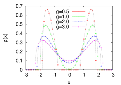
Figure 1: The eigenvalue distribution $\rho(x)$ is plotted for $g=0.5,1.0,2.0,3.0$ with $N=32$. The curves represent the exact results (6), (7) obtained in the planar large-$N$ limit.

Let us define the eigenvalue density distribution

$$\rho(x)\equiv\frac{1}{N}\Bigl{\langle}{\rm tr\,}\delta(x-\phi)\Bigr{\rangle}\ ,$$ (5)

from which one can calculate the expectation value of any single trace operator. In the planar limit the distribution $\rho(x)$ is obtained analytically [29] using the method developed in ref. [41]. For $g\geq 1$ the distribution is given by

$$\lim_{N\to\infty}\rho(x) = \frac{1}{\pi g}\left(\frac{1}{2}x^{2}+r^{2}-1\right)$$ (6)

$$\sqrt{4r^{2}-x^{2}}$$

in the range $-2r\leq x\leq 2r$, where $r^{2}=\frac{1}{3}(1+\sqrt{1+3g})$. For $g\leq 1$ it is given by

$$\lim_{N\to\infty}\rho(x)=\frac{1}{2\pi g}|x|\sqrt{(x^{2}-r_{-}^{2})(r_{+}^{2}-x^{2})}$$ (7)

in the range $r_{-}\leq|x|\leq r_{+}$, where $r_{\pm}^{2}=2(1\pm\sqrt{g})$. Outside the specified region, the distribution is constantly zero, and hence it has a compact support for $g\geq 1$, which splits into two for $g\leq 1$. This implies a phase transition of the Gross-Witten type [17] at the critical point

$$g=g_{\rm cr}\equiv 1\ .$$ (8)

Our Monte Carlo results for $N=32$ shown in fig. 1 agree well with the exact results in the planar limit.

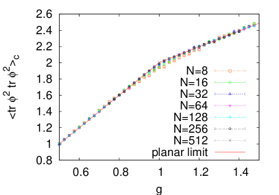
Figure 2: The two-point correlation function $\langle{\rm tr\,}\phi^{2}\,{\rm tr\,}\phi^{2}\rangle_{\rm c}$ is plotted against $g$ for various $N$. The solid line represents the analytic result (11) in the planar large-$N$ limit.

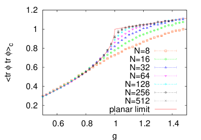
Figure 3: The two-point correlation function $\langle{\rm tr\,}\phi\,{\rm tr\,}\phi\rangle_{\rm c}$ is plotted against $g$ for various $N$. The solid line represents the analytic result (14) in the planar large-$N$ limit.

Let us next consider two-point correlation functions $\langle{\rm tr\,}\phi^{2}\,{\rm tr\,}\phi^{2}\rangle_{\rm c}$ and $\langle{\rm tr\,}\phi\,{\rm tr\,}\phi\rangle_{\rm c}$, where the suffix “c” implies that the connected part is taken. In the planar limit the correlation functions are obtained analytically as (See Appendix for derivation)

$$\lim_{N\to\infty}\langle{\rm tr\,}\phi^{2}\,{\rm tr\,}\phi^{2}\rangle_{\rm c} = \left\{\begin{array}[]{cc}\frac{2}{9}\left(1+\sqrt{1+3g}\right)^{2}&\textrm{for~{}}g\geq 1\ ,\\ 2g&\textrm{for~{}}g\leq 1\ .\\ \end{array}\right.$$ (11)

$$\lim_{N\to\infty}\langle{\rm tr\,}\phi\,{\rm tr\,}\phi\rangle_{\rm c} = \left\{\begin{array}[]{cc}\frac{1}{3}\left(1+\sqrt{1+3g}\right)&\textrm{for~{}}g\geq 1\ ,\\ 1-\sqrt{1-g}&\textrm{for~{}}g\leq 1\ .\\ \end{array}\right.$$ (14)

Our Monte Carlo results for various $N$ shown in figs. 3 and 3 approach the planar limit with increasing $N$.

In passing, let us consider the free energy of the system (1) defined by

$$F\equiv\log Z-\frac{1}{4}N^{2}\log g\ ,$$ (15)

where the log term is subtracted in order to make $F$ finite in the free case ($g=0$). One can easily see that the correlation function $\langle{\rm tr\,}\phi^{2}\,{\rm tr\,}\phi^{2}\rangle_{\rm c}$ is related to the second derivative of the free energy with respect to $g^{-1/2}$ as

$$\langle{\rm tr\,}\phi^{2}\,{\rm tr\,}\phi^{2}\rangle_{\rm c}=\frac{g}{N^{2}}\,\frac{\partial^{2}}{\partial(g^{-1/2})^{2}}\,F\ .$$ (16)

Therefore, the behavior (11) at the critical point $g=1$ implies that the phase transition is of third order in accord with ref. [17].

4 The double scaling limit

In this section we search for a double scaling limit, in which we send the coupling constant $g$ to the critical point $g_{\rm cr}=1$ simultaneously with the $N\rightarrow\infty$ limit keeping

$$\mu\equiv N^{p/3}(1-g)$$ (17)

fixed. We investigate whether the quantities

$$A(\mu,N) \equiv -N^{q/3}\Bigl{(}\langle{\rm tr\,}\phi^{2}\,{\rm tr\,}\phi^{2}\rangle_{\rm c}-2\Bigr{)}\ ,$$ (18)

$$B(\mu,N) \equiv -N^{r/3}\Bigl{(}\langle{\rm tr\,}\phi\,{\rm tr\,}\phi\rangle_{\rm c}-1\Bigr{)}$$ (19)

have large-$N$ limits as functions of $\mu$ for some choice of the parameters $p$, $q$ and $r$. In eqs. (18) and (19), we have subtracted the values in the planar large-$N$ limit at the critical point $g=1$, which are 2 and 1, respectively, for each correlation function; see, eqs. (11) and (14).

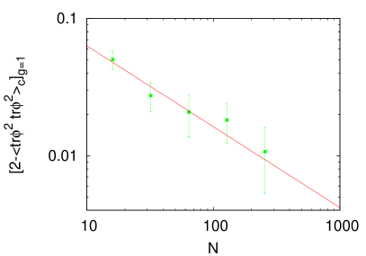
Figure 4: The observable $2-\langle{\rm tr\,}\phi^{2}\,{\rm tr\,}\phi^{2}\rangle_{\rm c}$ at the critical point $g=1$ is plotted against $N$ in the log-log scale. The straight line represents a fit to the power law behavior $N^{-1.7(3)}$.

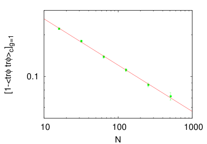
Figure 5: The observable $1-\langle{\rm tr\,}\phi\,{\rm tr\,}\phi\rangle_{\rm c}$ at the critical point $g=1$ is plotted against $N$ in the log-log scale. The straight line represents a fit to the power law behavior $N^{-1.00(2)}$.

In fact, by merely looking at the behavior of the planar results (11) and (14) near the critical point $g\sim 1$, one can readily deduce the existence of a double scaling limit for $\mu\sim\pm\infty$, where the $\pm$ sign corresponds to the behavior for $g\rightarrow 1\pm\epsilon$, respectively. Namely, plugging $g=1-\mu N^{-p/3}$ into (11) and (14), one obtains

$$\lim_{N\to\infty}A(\mu,N) = \left\{\begin{array}[]{cc}2\mu&\textrm{for~{}}\mu\sim\infty\ ,\\ \mu&\textrm{for~{}}\mu\sim-\infty\ ,\end{array}\right.$$ (22)

$$\lim_{N\to\infty}B(\mu,N) = \left\{\begin{array}[]{cc}\sqrt{\mu}&\textrm{for~{}}\mu\sim\infty\ ,\\ 0&\textrm{for~{}}\mu\sim-\infty\ ,\end{array}\right.$$ (25)

$$\mbox{~{}~{}with~{}~{}}q=p\quad{\rm and}\quad r=\frac{p}{2}\ .$$ (26)

When we search for a double scaling limit, we have to impose (26) in order to ensure the scaling behavior at large $|\mu|$. The nontrivial question then is whether we can choose the parameters within the constraints (26) in such a way that the scaling extends to small $|\mu|$. In general, the planar results can be used in this way to impose some constraints on the parameters that appear in searching for a double scaling limit. A similar strategy has been used, for instance, in ref. [16, 9, 10]. We emphasize, however, that this is just meant to make the analysis simpler, and that the relation (26) would come out anyway when we attempt to optimize the scaling behavior at large $|\mu|$.

Let us search for a scaling behavior at the particular point $\mu=0$. This corresponds to $g=1$ for any choice of $p$ due to (17), and therefore, we can actually determine $q$ and $r$ without using (26). In fig. 5 we plot the r.h.s. of (18) omitting the factor $N^{q/3}$. The observed power behavior implies $q=1.7(3)$. Similarly from fig. 5, we obtain $r=1.00(2)$. Using this value of $r$, the other exponents $p$ and $q$ may be obtained from the relation (26) as $p=q=2.00(4)$. This is consistent with the value of $q$ extracted from fig. 5 directly. The latter has a larger error bar, though. The reason for this is that the quantities plotted in figs. 5 and 5 are of the order of $\frac{1}{N^{2}}$ and $\frac{1}{N}$, respectively.

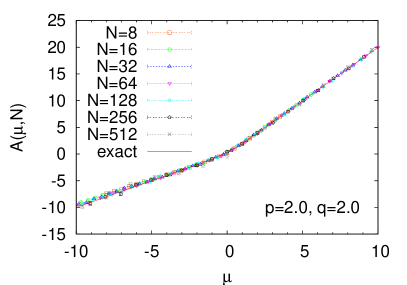
Figure 6: The quantity $A(\mu,N)$ is plotted against $\mu$ for $N=8,16,\cdots,512$ with $p=q=2.0$. The solid line represents the result (34) obtained in the double scaling limit.

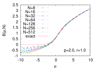
Figure 7: The quantity $B(\mu,N)$ is plotted against $\mu$ for $N=8,16,\cdots,512$ with $p=2.0$ and $r=1.0$. The solid line represents the result (35) obtained in the double scaling limit.

Now let us see whether these values of $p$, $q$ and $r$ make the quantities $A(\mu,N)$ and $B(\mu,N)$ scale also for $\mu\neq 0$. Using the Monte Carlo data shown in fig. 3, we plot the quantities as functions of $\mu$. Figs. 7 and 7 show the results. The scaling functions given below in eqs. (34) and (35) are also plotted for comparison. The Monte Carlo results for $A(\mu,N)$ show a nice scaling behavior, and they agree with the prediction (34). On the other hand, the quantity $B(\mu,N)$ scales and agrees with the prediction (35) only in the $\mu\gtrsim 0$ region. In the $\mu\lesssim 0$ region, we observe some tendency towards scaling as $N$ increases up to $N=512$, but the convergence to the prediction (35) seems to be slow. This behavior is due to the next-leading $1/N$ corrections, as we discuss in the next section.

In fact the analysis based on the orthogonal polynomial technique [5, 6, 7] suggests the existence of a double scaling limit with

$$p=q=2\quad{\rm and}\quad r=1\ ,$$ (27)

which agrees with our observation. In this limit the model (2) is conjectured [28] to be a dual description of the $\hat{c}=0$ noncritical string theory, where the parameter $\mu$ is identified with the cosmological constant in the corresponding super Liouville theory. Note that we are able to deduce the existence of the double scaling limit only from Monte Carlo data.

Let us also note that due to eq. (16), $A(\mu,N)$ is related to the “specific heat”

$$C(\mu,N)\equiv\frac{\partial^{2}F}{\partial\mu^{2}}-\left.\frac{\partial^{2}F}{\partial\mu^{2}}\right|_{\mu=0}$$ (28)

as

$$A(\mu,N)=-\frac{1}{4}\,N^{(q+2p-6)/3}\left\{C(\mu,N)+{\rm O}\left(N^{-2p/3}\right)\right\}\ .$$ (29)

Therefore, the scaling of $A(\mu,N)$ with the choice (27) implies that the “specific heat”, which has a physical meaning in the dual string theory, becomes finite in the double scaling limit.

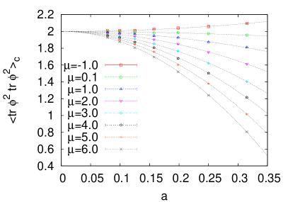
Figure 8: The observable $\langle{\rm tr\,}\phi^{2}\,{\rm tr\,}\phi^{2}\rangle_{\rm c}$ is plotted against $a(\equiv N^{-1/3})$ for various $\mu$ with $N=32,64,\cdots,2048$. For each $\mu$ we fit the data to the behavior (30) without the ${\rm O}(a^{4})$ terms treating $h(\mu)$ as a fitting parameter.

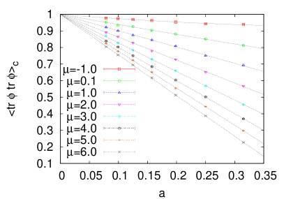
Figure 9: The observable $\langle{\rm tr\,}\phi\,{\rm tr\,}\phi\rangle_{\rm c}$ is plotted against $a(\equiv N^{-1/3})$ for various $\mu$ with $N=32,64,\cdots,2048$. For each $\mu$ we fit the data to the behavior (31) without the ${\rm O}(a^{3})$ terms treating $h(\mu)$ as a fitting parameter.

5 Next-leading $1/N$ corrections

So far we have been analyzing our Monte Carlo data without using the knowledge obtained from analytical results. The purpose of this section is to discuss more detailed behaviors in the double scaling limit which are obtained analytically, and to see whether our Monte Carlo data reproduce those behaviors as well.

As we briefly review in the Appendix, one can actually derive the asymptotic large-$N$ behavior of the correlation functions (for even $N$) in the double scaling limit as

$$\langle{\rm tr\,}\phi^{2}\,{\rm tr\,}\phi^{2}\rangle_{\rm c} = 2-\Bigl{\{}\mu+h^{2}(\mu)\Bigr{\}}a^{2}-\frac{1}{2}\Bigl{\{}\mu\,h(\mu)-h^{3}(\mu)\Bigr{\}}a^{3}+{\rm O}(a^{4})\ ,$$ (30)

$$\langle{\rm tr\,}\phi\,{\rm tr\,}\phi\rangle_{\rm c} = 1-h(\mu)\,a-\frac{1}{4}\Bigl{\{}\mu-h^{2}(\mu)\Bigr{\}}a^{2}+{\rm O}(a^{3})\ ,$$ (31)

where we have introduced a parameter $a\equiv N^{-1/3}$, and $h(\mu)$ is a function which satisfies the differential equation [42]

$$\mu\,h(\mu)=h^{3}(\mu)-2\,h^{\prime\prime}(\mu)\ ,$$ (32)

and the boundary conditions

$$h(\mu)\sim\left\{\begin{array}[]{cc}\sqrt{\mu}&\textrm{for~{}}\mu\sim\infty\ ,\\ 0&\textrm{for~{}}\mu\sim-\infty\ .\end{array}\right.$$ (33)

Equation (32) is nothing but the Painleve-II equation, which is proven [43] to have a unique real solution under the boundary conditions (33). The solution is obtained numerically in ref. [44] to high accuracy, and we use it in plotting the exact results in figs. 7, 7 and 10.

From (30) and (31), the large-$N$ limits of the quantities (18), (19) are obtained as

$$\lim_{N\to\infty}A(\mu,N) = \mu+h^{2}(\mu)\ ,$$ (34)

$$\lim_{N\to\infty}B(\mu,N) = h(\mu)\ ,$$ (35)

which we plot as exact results in figs. 7 and 7. Plugging in the boundary conditions (33), we reproduce eqs. (22) and (25) obtained from the planar results.

The analysis in the previous section therefore amounts to extracting the leading $1/N$ corrections in (30) and (31). The reason for the observed slow approach to the limit (35) for $\mu\lesssim 0$ is that the coefficient of the O($a$) term in the expansion (31) becomes much smaller than that of the O($a^{2}$) term as $\mu$ decreases due to the boundary conditions (33).

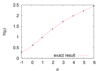
Figure 10: The crosses and the circles represent the function $h(\mu)$, which is extracted from figs. 9 and 9, respectively. The solid line represents the solution of the Painleve-II equation.

It would therefore be interesting to see whether the next-leading $1/N$ corrections in eqs. (30) and (31) are reproduced by Monte Carlo simulation. In fig. 9 we plot $\langle{\rm tr\,}\phi^{2}\,{\rm tr\,}\phi^{2}\rangle_{\rm c}$ against $a$ for various $\mu$. Indeed the data can be nicely fitted to the behavior (30) without the ${\rm O}(a^{4})$ terms, where $h(\mu)$ is determined as a fitting parameter by optimizing the fit for each $\mu$. In fig. 9 we plot the observable $\langle{\rm tr\,}\phi\,{\rm tr\,}\phi\rangle_{\rm c}$ against $a$ for various $\mu$. Again the data can be nicely fitted to the behavior (31) without the ${\rm O}(a^{3})$ terms, where $h(\mu)$ is determined similarly. The function $h(\mu)$ obtained in this way is plotted in fig. 10. The crosses and the circles represent the results obtained from $\langle{\rm tr\,}\phi^{2}\,{\rm tr\,}\phi^{2}\rangle_{\rm c}$ and $\langle{\rm tr\,}\phi\,{\rm tr\,}\phi\rangle_{\rm c}$, respectively, which turn out to be consistent with each other within error bars. Furthermore the results agree with the solution of the Painleve-II equation (32) with the boundary conditions (33).

6 Summary

In this paper we have shown how one can use Monte Carlo simulation to search for a double scaling limit, and, if it exists, to obtain the corresponding scaling functions. For that purpose we studied a solvable one-matrix model which has recently been proposed as a constructive formulation of noncritical strings with worldsheet supersymmetry. In particular, we have shown how the results in the planar limit provide useful information in such an investigation. The required matrix size is not very large in most cases, but we have also encountered a case in which the approach to the large-$N$ limit turns out to be slow due to large next-leading $1/N$ corrections.

Considering that even a simple two-matrix model are not solvable except for some special cases [45], we believe that Monte Carlo simulation provides a powerful tool to investigate the universality class of matrix models in the double scaling limit. For instance, in ref. [46] a string field theory of minimal $(p,q)$ superstrings has been constructed from the two-cut ansatz for the two-matrix model. It would be interesting to confirm their results by taking the double scaling limit explicitly.

In general, if there exists a continuous phase transition in the planar limit, one has a chance to take the double scaling limit by approaching the critical point with increasing $N$. How generically this holds needs to be investigated. For instance, it is known that the unitary matrix model [17] has a third order phase transition, which allows a double scaling limit [47]. The obtained limit belongs to the same universality class [42] as the one studied in this paper. Whether a double scaling limit defines a sensible nonperturbative string theory is also an important issue, which was addressed in refs. [23, 48, 49] by Monte Carlo simulation. We hope that Monte Carlo studies of matrix models will also shed light on nonperturbative dynamics of critical strings.

Appendix A Derivation of the asymptotic behaviors (30) and (31)

The prediction for the present model is obtained by the orthogonal-polynomial technique, which is a powerful tool to calculate various quantities in the double scaling limit (see [50] for a review). In this Appendix we briefly review the derivation of the asymptotic behaviors (30) and (31) for the reader’s convenience.

Using the orthogonal-polynomial method, various quantities in the matrix model can be expressed in terms of the coefficients $R_{n}\ (n=1,2,3,\cdots)$ characterized by the recursion formula

$$g\,\frac{n}{N} = R_{n}\,(-2+R_{n+1}+R_{n}+R_{n-1})\ .$$ (36)

For example, the correlation functions defined by eqs. (30) and (31) are expressed as

$$\langle{\rm tr\,}\phi^{2}\,{\rm tr\,}\phi^{2}\rangle_{\rm c} = R_{N}\,(R_{N+1}+R_{N-1})\ ,$$ (37)

$$\langle{\rm tr\,}\phi\,{\rm tr\,}\phi\rangle_{\rm c} = R_{N}\ .$$ (38)

In the planar limit (i.e., the $N\rightarrow\infty$ limit with fixed $g$), the asymptotic behavior of the coefficients $R_{n}$ is given by

$$R_{n}=\left\{\begin{array}[]{cc}\frac{1}{3}\left(1+\sqrt{1+3\xi}\right)&\textrm{for }\xi\geq 1\ ,\\ 1-(-1)^{n}\sqrt{1-\xi}&\textrm{for }\xi\leq 1\ ,\\ \end{array}\right.$$ (41)

where $\xi=gn/N$ is regarded as a continuous variable. Note that, for $\xi\leq 1$, the asymptotic behavior of $R_{n}$ is given by two continuous functions depending on the parity of $n$. By plugging (41) into (37) and (38), one obtains the planar results (11) and (14).

Next we consider the double scaling limit; i.e., the $N\rightarrow\infty$ limit with fixed $\mu$ defined by (17) with $p=2$. This implies that the coupling constant $g$ approaches the critical point $g_{\rm cr}\equiv 1$ as

$$g=1-\mu a^{2}\ ,$$ (42)

where we have defined $a\equiv N^{-1/3}$ as before. In order to obtain the asymptotic behaviors of (37) and (38) in that limit, we need to know the behavior of the coefficient $R_{n}$ for the region of $n$, which can be parametrized as

$$\xi = g\,\{1-(t-\mu)a^{2}\}$$ (43)

$$= 1-ta^{2}+{\rm O}(a^{4})$$

using the new variable $t$. For large $|t|$, we can deduce the asymptotic behavior of $R_{n}$ from the planar result (41). Namely, by plugging (43) into (41) and by expanding it with respect to $a$, we obtain

$$R_{n}=\left\{\begin{array}[]{cc}1-\frac{t}{4}a^{2}+{\rm O}(a^{4})&\textrm{for~{}}t\sim-\infty\ ,\\ 1-(-1)^{n}\sqrt{t}a+{\rm O}(a^{3})&\textrm{for~{}}t\sim\infty\ .\end{array}\right.$$ (46)

This motivates us to adopt the Ansatz [51, 42]

$$R_{n}=1-(-1)^{n}H(t)\,a+F(t)\,a^{2}\ ,$$ (47)

where $H(t)$ and $F(t)$ are regarded as continuous functions of $t$, which can be expanded with respect to $a$ as

$$H(t) = h(t)+{\rm O}(a^{2})\ ,$$ (48)

$$F(t) = f(t)+{\rm O}(a^{2})\ .$$ (49)

Substituting the Ansatz (47) into (36), we obtain

$$h^{\prime\prime}(t) = 2\,f(t)\,h(t)\ ,$$ (50)

$$h^{2}(t) = 4\,f(t)+t$$ (51)

as consistency conditions. Eliminating $f(t)$, we obtain the Painleve-II equation (32). The asymptotic behavior (46) translates into the boundary condition (33). Plugging (47) into eqs. (37) and (38), we obtain the asymptotic behaviors (30) and (31).

References

- [1] G. ’t Hooft, A planar diagram theory for strong interactions, Nucl. Phys. B 72 (1974) 461.
- [2] O. Aharony, S. S. Gubser, J. M. Maldacena, H. Ooguri and Y. Oz, Large N field theories, string theory and gravity, Phys. Rept. 323 (2000) 183 [hep-th/9905111].
- [3] R. Gopakumar and C. Vafa, On the gauge theory/geometry correspondence, Adv. Theor. Math. Phys. 3 (1999) 1415 [hep-th/9811131] ; R. Dijkgraaf and C. Vafa, Matrix models, topological strings, and supersymmetric gauge theories, Nucl. Phys. B 644 (2002) 3 [hep-th/0206255].
- [4] M. Kontsevich, Intersection theory on the moduli space of curves and the matrix Airy function, Commun. Math. Phys. 147 (1992) 1.
- [5] E. Brezin and V. A. Kazakov, Exactly solvable field theories of closed strings, Phys. Lett. B 236 (1990) 144.
- [6] M. R. Douglas and S. H. Shenker, Strings in less than one-dimension, Nucl. Phys. B 335 (1990) 635.
- [7] D. J. Gross and A. A. Migdal, Nonperturbative two-dimensional quantum gravity, Phys. Rev. Lett. 64 (1990) 127.
- [8] G. Bertoldi, Double scaling limits and twisted non-critical superstrings, J. High Energy Phys. 0607 (2006) 006 [hep-th/0603075]; G. Bertoldi, T. J. Hollowood and J. L. Miramontes, Double scaling limits in gauge theories and matrix models, J. High Energy Phys. 0606 (2006) 045 [hep-th/0603122]; M. Alimohammadi and M. Khorrami, Phase transitions of large-N two-dimensional Yang-Mills and generalized Yang-Mills theories in the double scaling limit, Eur. Phys. J. C 47 (2006) 507 [hep-th/0604027]; L. Alvarez-Gaume, P. Basu, M. Marino and S. R. Wadia, Blackhole/string transition for the small Schwarzschild blackhole of AdS5 S5 and critical unitary matrix models, Eur. Phys. J. C 48 (2006) 647 [hep-th/0605041].
- [9] W. Bietenholz, F. Hofheinz and J. Nishimura, The renormalizability of 2D Yang-Mills theory on a non-commutative geometry, J. High Energy Phys. 0209 (2002) 009 [hep-th/0203151].
- [10] W. Bietenholz, F. Hofheinz and J. Nishimura, Phase diagram and dispersion relation of the non-commutative lambda model in d = 3, J. High Energy Phys. 0406 (2004) 042 [hep-th/0404020].
- [11] W. Bietenholz, J. Nishimura, Y. Susaki and J. Volkholz, A non-perturbative study of 4d U(1) non-commutative gauge theory: The fate of one-loop instability, J. High Energy Phys. 0610 (2006) 042 [hep-th/0608072].
- [12] T. Banks, W. Fischler, S. H. Shenker and L. Susskind, M theory as a matrix model: A conjecture, Phys. Rev. D 55 (1997) 5112 [hep-th/9610043].
- [13] N. Ishibashi, H. Kawai, Y. Kitazawa and A. Tsuchiya, A large-N reduced model as superstring, Nucl. Phys. B 498 (1997) 467 [hep-th/9612115].
- [14] R. Dijkgraaf, E. Verlinde and H. Verlinde, Matrix string theory, Nucl. Phys. B 500 (1997) 43 [hep-th/9703030].
- [15] T. Eguchi and H. Kawai, Reduction of dynamical degrees of freedom in the large N gauge theory, Phys. Rev. Lett. 48 (1982) 1063.
- [16] T. Nakajima and J. Nishimura, Numerical study of the double scaling limit in two-dimensional large N reduced model, Nucl. Phys. B 528 (1998) 355 [hep-th/9802082].
- [17] D. J. Gross and E. Witten, Possible third order phase transition in the large N Lattice gauge theory, Phys. Rev. D 21 (1980) 446.
-
[18]
A. González-Arroyo and M. Okawa,
A twisted model for large lattice gauge theory,
Phys. Lett. B 120 (1983) 174;
The twisted Eguchi-Kawai model: a reduced model for large N
lattice gauge theory,
Phys. Rev. D 27 (1983) 2397.
- [19] J. Ambjørn, Y.M. Makeenko, J. Nishimura and R.J. Szabo, Finite N matrix models of noncommutative gauge theory, J. High Energy Phys. 11 (1999) 029 [hep-th/9911041]; Nonperturbative dynamics of noncommutative gauge theory, Phys. Lett. B 480 (2000) 399 [hep-th/0002158]; Lattice gauge fields and discrete noncommutative Yang-Mills theory, J. High Energy Phys. 05 (2000) 023 [hep-th/0004147].
- [20] S. Minwalla, M. van Raamsdonk and N. Seiberg, Noncommutative perturbative dynamics, J. High Energy Phys. 02 (2000) 020 [hep-th/9912072].
- [21] J. Ambjorn, K. N. Anagnostopoulos, W. Bietenholz, T. Hotta and J. Nishimura, Monte Carlo studies of the IIB matrix model at large N, J. High Energy Phys. 0007 (2000) 011 [hep-th/0005147].
- [22] K. N. Anagnostopoulos and J. Nishimura, New approach to the complex-action problem and its application to a nonperturbative study of superstring theory, Phys. Rev. D 66 (2002) 106008 [hep-th/0108041].
- [23] J. Ambjorn, K. N. Anagnostopoulos, W. Bietenholz, T. Hotta and J. Nishimura, Large N dynamics of dimensionally reduced 4D SU(N) super Yang-Mills theory, J. High Energy Phys. 0007 (2000) 013 [hep-th/0003208].
- [24] J. McGreevy and H. L. Verlinde, Strings from tachyons: The c = 1 matrix reloaded, J. High Energy Phys. 0312 (2003) 054 [hep-th/0304224].
- [25] I. R. Klebanov, J. M. Maldacena and N. Seiberg, D-brane decay in two-dimensional string theory, J. High Energy Phys. 0307 (2003) 045 [hep-th/0305159].
- [26] T. Takayanagi and N. Toumbas, A matrix model dual of type 0B string theory in two dimensions, J. High Energy Phys. 0307 (2003) 064 [hep-th/0307083].
- [27] M. R. Douglas, I. R. Klebanov, D. Kutasov, J. M. Maldacena, E. Martinec and N. Seiberg, A new hat for the c = 1 matrix model, hep-th/0307195.
- [28] I. R. Klebanov, J. M. Maldacena and N. Seiberg, Unitary and complex matrix models as 1-d type 0 strings, Commun. Math. Phys. 252 (2004) 275 [hep-th/0309168].
- [29] G. M. Cicuta, L. Molinari and E. Montaldi, Large N phase transitions in low dimensions, Mod. Phys. Lett. A 1 (1986) 125.
- [30] H. Kawai, T. Kuroki and Y. Matsuo, Universality of nonperturbative effect in type 0 string theory, Nucl. Phys. B 711 (2005) 253 [hep-th/0412004].
- [31] M. Hanada, M. Hayakawa, N. Ishibashi, H. Kawai, T. Kuroki, Y. Matsuo and T. Tada, Loops versus matrices: The nonperturbative aspects of noncritical string, Prog. Theor. Phys. 112 (2004) 131 [hep-th/0405076].
- [32] A. Sato and A. Tsuchiya, ZZ brane amplitudes from matrix models, J. High Energy Phys. 0502 (2005) 032 [hep-th/0412201].
- [33] N. Ishibashi, T. Kuroki and A. Yamaguchi, Universality of nonperturbative effects in noncritical string theory, J. High Energy Phys. 0509 (2005) 043 [hep-th/0507263].
- [34] Y. Matsuo, Nonperturbative effect in c = 1 noncritical string theory and Penner model, Nucl. Phys. B 740 (2006) 222 [hep-th/0512176].
- [35] R. de Mello Koch, A. Jevicki and J. P. Rodrigues, Instantons in c = 0 CSFT, J. High Energy Phys. 0504 (2005) 011 [hep-th/0412319].
- [36] N. Ishibashi and A. Yamaguchi, On the chemical potential of D-instantons in c = 0 noncritical string theory, J. High Energy Phys. 0506 (2005) 082 [hep-th/0503199].
- [37] M. Fukuma, H. Irie and S. Seki, Comments on the D-instanton calculus in (p,p+1) minimal string theory, Nucl. Phys. B 728 (2005) 67 [hep-th/0505253].
- [38] T. Kuroki and F. Sugino, T duality of the Zamolodchikov-Zamolodchikov brane, Phys. Rev. D 75 (2007) 044008 [hep-th/0612042].
- [39] X. Martin, A matrix phase for the scalar field on the fuzzy sphere, J. High Energy Phys. 0404 (2004) 077 [hep-th/0402230]; F. Garcia Flores, D. O’Connor and X. Martin, Simulating the scalar field on the fuzzy sphere, PoS LAT2005 (2006) 262 [hep-lat/0601012].
- [40] M. Panero, Numerical simulations of a non-commutative theory: The scalar model on the fuzzy sphere, hep-th/0608202; Quantum field theory in a non-commutative space: Theoretical predictions and numerical results on the fuzzy sphere, SIGMA 2 (2006), 081 [hep-th/0609205].
- [41] E. Brezin, C. Itzykson, G. Parisi and J. B. Zuber, Planar diagrams, Commun. Math. Phys. 59 (1978) 35.
- [42] M. R. Douglas, N. Seiberg and S. H. Shenker, Flow and instability in quantum gravity, Phys. Lett. B 244 (1990) 381.
- [43] S. Hastings and J. McLeod, A boundary value problem associated with the second Painleve transcendent and the Korteweg de Vries equation, Arch. Rational Mech. Anal. 73 (1980) 31.
- [44] M. Praehofer and H. Spohn, Exact scaling functions for one-dimensional stationary KPZ growth, J. Stat. Phys. 115(1-2) (2004) 255 [cond-mat/0212519].
- [45] C. Itzykson and J. B. Zuber, The planar approximation. 2, J. Math. Phys. 21 (1980) 411.
- [46] M. Fukuma and H. Irie, A string field theoretical description of (p,q) minimal superstrings, J. High Energy Phys. 0701 (2007) 037 [hep-th/0611045].
- [47] V. Periwal and D. Shevitz, Unitary matrix models as exactly solvable string theories, Phys. Rev. Lett. 64 (1990) 1326.
- [48] K. N. Anagnostopoulos, W. Bietenholz and J. Nishimura, The area law in matrix models for large N QCD strings, Int. J. Mod. Phys. C 13 (2002) 555 [hep-lat/0112035].
- [49] M. Hanada, H. Kawai, T. Kanai and F. Kubo, Phase structure of the large-N reduced gauge theory and generalized Weingarten model, Prog. Theor. Phys. 115 (2006) 1167 [hep-th/0604065]; M. Hanada and F. Kubo, String tension and string susceptibility in two-dimensional generalized Weingarten model, hep-th/0611207.
- [50] P. Di Francesco, P. H. Ginsparg and J. Zinn-Justin, 2-D Gravity and random matrices, Phys. Rept. 254 (1995) 1 [hep-th/9306153].
- [51] C. Crnkovic and G. W. Moore, Multicritical multicut matrix models, Phys. Lett. B 257 (1991) 322.
- [52] C. Crnkovic, M. R. Douglas and G. W. Moore, Physical solutions for unitary matrix models, Nucl. Phys. B 360 (1991) 507.