Landscape Predictions from Cosmological Vacuum Selection

Abstract

In BP models with hundreds of fluxes, we compute the effects of cosmological dynamics on the probability distribution of landscape vacua. Starting from generic initial conditions, we find that most fluxes are dynamically driven into a different and much narrower range of values than expected from landscape statistics alone. Hence, cosmological evolution will access only a tiny fraction of the vacua with small cosmological constant. This leads to a host of sharp predictions. Unlike other approaches to eternal inflation, the holographic measure employed here does not lead to “staggering”, an excessive spread of probabilities that would doom the string landscape as a solution to the cosmological constant problem.

I Introduction

The task of making predictions in the landscape of string theory represents an enormous challenge. We must survey the metastable vacua in the theory and find the relative abundance of various low-energy properties. But vacua without observers will not be observed. The great variability of low energy physics in the string landscape demands novel methods for capturing such selection effects.

Interposed between these two tasks is a third problem, which will be the focus of this paper: vacuum selection by cosmological dynamics. It is not enough for a vacuum to exist in theory. It will be relevant only if it can be dynamically realized from generic initial conditions, either as regions in spacetime or branches of a wavefunction.

The former viewpoint insists on treating spacetime semiclassically on a global scale. This has no operational meaning, since no observer can see beyond his own horizon BouFre06a . Moreover, it leads to problematic infinities and ambiguities that have plagued the definition of measures in eternal inflation; see, e.g., Refs. LinLin94 ; GarLin94 ; GarVil01 ; GarSch05 ; EasLim05 ; Bou06 ; Bou06b for discussions and some recent proposals. Thus, the global viewpoint seems poised to suffer the same fate as the ether: a false convenience increasingly recognized as a burden. (A similar conclusion was reached earlier by studying quantum aspects of black holes SusTho93 ; Pre92 , and it seems natural indeed that it should extend to cosmology.)

One of us recently proposed a “holographic” measure Bou06 that refers only to a single causally connected region, or causal diamond. In Ref. BouHar07 , it was shown that this measure not only overcomes problems that plagued anthropic predictions of the cosmological constant, but is able to maintain this success when specific anthropic conditions are traded for the much weaker assumption that observers require merely free energy.

Here we apply a different aspect of the proposal of Ref. Bou06 . We focus not on anthropic selection, but on cosmological selection. We shall find that dynamical effects can significantly suppress or enhance the probability of observing a given vacuum, and they can interfere with anthropic selection in some models. However, unlike another recently proposed measure GarSch05 , the holographic measure does not lead to excessively uneven probability distributions that would render the string landscape ineffective at solving the cosmological constant problem.

We will follow Ref. BP in modelling the string landscape as arising from a large number of possible four-form flux configurations. We mainly consider a model with $250$ fluxes, with fixed charges of order $1/30$. This yields a large number of metastable vacua, of which $10^{121}$ have vacuum energy comparable to the observed value. Of these, however, we find that only $10^{80}$ are accessed by a typical worldline, starting from generic initial conditions.

The selected ensemble is characterized by 250 probability distributions over the integers, one for each flux. The distributions differ—in many cases, drastically—from the distributions one would have obtained by simply restricting the landscape to vacua with small cosmological constant. Thus, cosmological selection leads to thousands of distinct predictions. Many correspond to probabilities that are so close to 0 or 1 that even a single conflicting observation would rule out the model.

The specific predictions we obtain apply only to the toy model we study, but they do allow us to draw more general lessons. Most importantly, our results demonstrate that cosmological dynamics can be a powerful constraint. It reduces the effective size of the landscape drastically, leading to a large number of strong predictions. Another general lesson is that fast decays happen first. In natural models, it takes hundreds or thousands of tunneling events to get from a generic initial vacuum to a vacuum with observers. Any metastable internal configuration that gives rise to a relatively fast decay channel but is unlikely to arise late in the decay chain will not be observed.

In the real string landscape, the selection effects will likely be as strong as in the BP models studied here, but they may be harder to characterize in terms of a set of nearly independent flux distributions. For example, charges will not be independent of fluxes, and their dynamical effects can become intertwined.

The specific flux configuration associated with our own vacuum is unlikely to be observed directly in the near future. However, fluxes are related to coupling constants and other low-energy parameters. It will be important to understand such correlations in realistic and representative sets of string compactifications. Then it will be possible to understand the impact of cosmological selection effects on the distribution of low-energy parameters.

Outline

Sec. II includes brief descriptions of the BP model, and of the holographic cosmological probability measure we use to compute cosmological selection effects. We focus on the question of how this measure can be effectively applied to a model with ten to the hundreds of vacua. This would seem to require inverting a matrix of the corresponding rank. However, we develop statistical methods that are both adequate and very efficient. (Details of the techniques are given in Appendices A and B.) We also discuss our choice of initial conditions, and we show that our results will be the same for any initial probability distribution that depends only on $\lambda$ and does not strongly favor small or negative values of $\lambda$.

In Sec. III, we present our results. For a representative model, we contrast the distribution of fluxes, and the number of vacua with small cosmological constant, before and after cosmological selection effects are taken into account. We point out specific predictions that can be made with high confidence, focussing on features that would have been either absent or strikingly different if cosmological dynamics had been neglected. We consider other models to illustrate that the strength of cosmological selection effects varies and that, in special cases, a model that naively contains enough vacua may fail after cosmological selection is accounted for.

In Sec. IV, we try to give a qualitative explanation of the features seen in the cosmological flux distribution. We identify them as imprints of the dynamics at different stages in the decay chain, when different types of transitions dominate.

In Sec. V, we compare our results to those obtained by Schwartz-Perlov and Vilenkin SchVil06 from a different proposal for the probability measure GarSch05 . In toy-BP-models with fewer vacua, the alternative measure leads to a “staggered” probability distribution, which would leave the string landscape effectively underpopulated and unable to solve the cosmological constant problem. The measure of Ref. GarSch05 is difficult to apply explicitly in models with a realistic number of vacua, and to extend beyond first order in perturbation theory. However, we show in Appendix C that it is equivalent to the holographic measure with particular (and from our point of view, highly unnatural) initial conditions. With the help of this trick, we are able to argue that the staggering problem is likely to persist at higher orders when the measure of Ref. GarSch05 is applied to large BP models.

II Model and measure

II.1 Probability measure, course graining, and Monte Carlo chains

Consider a worldline starting in some metastable initial vacuum. This vacuum will eventually decay, giving way to a new vacuum. The cascade continues until the worldline enters a terminal vacuum, which does not decay further. According to the proposal of Ref. Bou06 , the probability $P_{A}$ assigned to vacuum $A$ is the expected number of times the worldline will enter vacuum $A$ on its way down to a terminal vacuum. For a more general initial probability distribution $P_{A}^{(0)}$, one sums over the result obtained from each initial vacuum, weighted by $P_{A}^{(0)}$.

The probabilities $P_{A}$ form an ${\cal N}$-dimensional vector, where ${\cal N}$ is the number of vacua in the landscape. It satisfies the matrix equation Bou06

$$(1-\eta)\mathbf{P}=\eta\mathbf{P}^{(0)}~{}.$$ (1)

where $\eta_{AB}$ is the relative decay rate, or branching ratio, from vacuum $B$ into vacuum $A$. It can be obtained from the decay rate per unit time, $\kappa_{AB}$, by normalizing each column of $\kappa_{AB}$,

$$\eta_{AB}=\frac{\kappa_{AB}}{\sum_{C}\kappa_{CB}}~{},$$ (2)

except for columns corresponding to terminal vacua (which vanish both for $\kappa$ and for $\eta$).

In a large landscape, one expects that both the initial distribution, $P_{A}^{(0)}$, and the distribution resulting from dynamical selection, $P_{A}$, will have support over an enormous number of vacua. Then it is impractical to solve Eq. (1) in detail. But fortunately, the probability of a particular vacuum is no more interesting than that of a specific quantum state in a macroscopic system. A more natural set of questions is the following: How large is the subset of vacua selected by cosmological dynamics, and how can it be characterized?

In fact, we will ask a more restrictive set of questions. Let us suppose that vacua with $\lambda\gg\lambda_{0}$ contain no observers, where

$$\lambda_{0}\approx 7.9\times 10^{-121}$$ (3)

is the observed cosmological constant. Then we may restrict our attention to vacua with cosmological constant $\lambda$ of order the observed value:

$$0<\lambda\lesssim\lambda_{0}~{}.$$ (4)

(For simplicity, we exclude negative values of $\lambda$; this will make our formulas simpler without changing our results qualitatively. For the same reason, we will take the upper bound to be sharp.) We will consider only models which contain a large number of such vacua, and we will be interested in the restriction of the probability distribution $P_{A}$ to this subset of vacua. Thus, we ask:

• How large is the set of vacua which (a) satisfy Eq. (4) and (b) are selected by cosmological dynamics?

• What characteristics distinguish typical vacua in the above set from typical vacua which merely satisfy (a)?

Instead of solving Eq. (1), we will approach these questions by a Monte Carlo simulation. We select an unbiased sample of $N$ initial vacua according to a generic initial distribution $P_{A}^{(0)}$. For each initial vacuum, we simulate a decay chain: At every step, a new vacuum $B$ is selected with a probability given by the branching ratios, $\eta_{AB}$, where $B$ is the old vacuum. The chain will eventually reach a terminal vacuum, i.e., a vacuum with negative cosmological constant. We are interested in the penultimate vacuum, which still has positive vacuum energy. For large enough $N$, the penultimate vacua obtained from the Monte Carlo simulation become a representative sample of the ensemble of vacua selected from the landscape by cosmological dynamics.

II.2 BP model and decay rates

We will follow Ref. BP in modeling the string landscape as a set of flux vacua, neglecting the backreaction of fluxes and moduli stabilization. The geometry is of the form $M_{4}\times X$, where $X$ is a compact 6 or 7-dimensional manifold, and $M_{4}$ is the macroscopic four-dimensional spacetime. A $p$-brane wrapped on a $p-2$ cycle in $X$ acts as a membrane in $M_{4}$. The number of cycles, $J$, and thus the number of membrane species, can range into the hundreds. Each species sources a four-form field strength in $M_{4}$. The four-form flux is quantized, so each vacuum is fully specified by the set $\{n_{i}\}$, $i=1,\ldots,J$, of integer flux numbers. The vacua form a $J$ dimensional grid in flux space (Fig. 1).

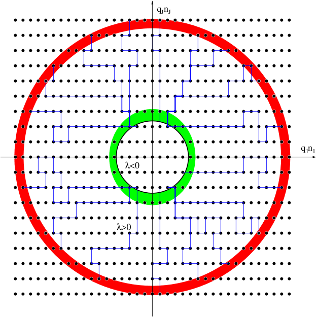
Figure 1: A two-dimensional slice through the $J$-dimensional flux grid. Surfaces of constant $\lambda$ are $J-1$ dimensional spheres. Each dot represents a vacuum. Starting from initial vacua with $\lambda\approx 1$ (outermost shell), we simulate decay chains (blue lines) through the landscape, which terminate when a vacuum with $\lambda\leq 0$ is reached. Among the “penultimate” vacua with relatively small positive $\lambda$ (green/shaded region), only a small fraction is actually accessed by the decay chains, leading to a host of predictions. Vacua with $\lambda$ of order the tiny observed value lie in a much thinner shell (schematically shown as a black circle). A model can be ruled out if the selection effects render this shell inaccessible.

The cosmological constant can be written as

$$\lambda=\lambda_{\rm bare}+\frac{1}{2}\sum^{J}_{i=1}n_{i}^{2}q_{i}^{2}~{},$$ (5)

Here, $q_{i}$ is the charge of the $i$-th membrane. The second term is contributed by the $J$ species of four-form flux. $\lambda_{\rm bare}$ subsumes all other contributions, in particular those from vacuum loops, and will be assumed to be naturally large and negative:

$$-\lambda_{\rm bare}=O(1)~{}.$$ (6)

If each flux can take several different integer values, then there will be an enormous number of vacua. Some of these vacua will accidentally have a very small cosmological constant, even though no small scale is introduced into the model. If the model contains vacua with a cosmological constant on the order of the observed value in our universe, $\lambda_{0}$, then the cosmological constant problem can be solved by anthropic selection effects Wei87 ; Bou06 ; BouHar07 .

A more detailed model of the string landscape should include the backreaction of fluxes on the geometry (see Ref. DouKac06 for a review). These effects are still hard to control, especially if we are interested in the cosmology of a large, representative part of the landscape. In particular, both the charges $q_{i}$ and the bare cosmological constant would depend on the set $\{n_{i}\}$. However, this is unlikely to affect a key feature of the BP model: that the vacua form a discretuum with tiny effective spacing of the cosmological constant.

In general, a metastable vacuum can decay to any other vacuum. However, a typical decay will change one flux by one unit. Tunneling events that change more than one flux, or change a flux by more than one unit, can be regarded as a composite event. They will be much more suppressed than one of their constituent events and can thus be neglected. This simplifies our task, reducing the number of possible decays at each step to $2J$. The only question is which flux will change, and in which direction.

The relative decay rates are given by Eq. (2), with

$$\kappa_{ij}=A_{j}e^{-B_{ij}}~{}.$$ (7)

The constant $A_{j}$ depends only on the host vacuum and drops out in the branching ratios. The instanton action for decreasing the magnitude of the $i$-th flux, $n_{i}$, by one unit is given by BroTei87

$$B(|n_{i}|\to|n_{i}|-1) = B_{\rm flat}(|n_{i}|\to|n_{i}|-1)\,r(x,y)$$

$$B_{\rm flat}(|n_{i}|\to|n_{i}|-1) = \frac{27\pi^{2}}{8}\frac{1}{\left(|n_{i}|-\frac{1}{2}\right)^{3}q_{i}^{2}}$$

$$r(x,y) = \frac{2[(1+xy)-\sqrt{1+2xy+x^{2}}]}{x^{2}(y^{2}-1)\sqrt{1+2xy+x^{2}}}$$

$$x = \frac{3}{8\left(|n_{i}|-\frac{1}{2}\right)}$$

$$y = \frac{2\lambda}{q_{i}^{2}\left(|n_{i}|-\frac{1}{2}\right)}-1~{},$$ (8)

where $\lambda$ is the cosmological constant in the first vacuum. Upward tunneling is further suppressed by the relative entropy of the two vacua:

$$B(|n_{i}|\to|n_{i}|+1)=$$

$$B(|n_{i}|+1\to|n_{i}|)\exp\left(\frac{24\pi^{2}}{\lambda+\left(|n_{i}|+\frac{1}{2}\right)q_{i}^{2}}-\frac{24\pi^{2}}{\lambda}\right) ~{}.$$

For fluxes with $n_{i}=0$ it is important to take into account that $0\to 1$ and $0\to-1$ are two distinct decay channels that contribute equal amounts to the total decay rate entering Eq. (2).

II.3 Quantifying selection effects

Given the $N$ vacua selected by our Monte Carlo simulation, we can answer the two questions posed above. First, let us focus on how the selected vacua can be characterized and distinguished from an unbiased ensemble of vacua with small cosmological constant.

In our toy model, the only variables we have available are the fluxes, $n_{i}$. A list of $J$ fluxes specifies a unique vacuum, but a list of $J$ probability distributions (one for each flux) defines an ensemble of vacua. Larger ensembles could be defined by throwing away more information, e.g., by specifying only a list of $J$ expectation values $\langle n_{i}\rangle$. However, we are interested in extracting as much information as possible from our simulation. Hence, we will consider the $J$ discrete distributions

$$p_{i}(n)\equiv\mbox{probability that the}~{}i\mbox{-th flux,}\,n_{i},$$

$$\mbox{has integer value}~{}n~{}.$$ (10)

Selection effects can be demonstrated by comparing the $J$ distributions obtained from the selected vacua, with the $J$ distributions obtained from an unbiased sample of vacua with a similar range of vacuum energy.

Next, let us turn to estimating the total number of selected vacua from the small sample obtained by the simulation, and comparing this to the total number of vacua in a similar range of vacuum energy. This task is slightly more subtle.

Associated with each probability distribution $p_{i}(n)$ is a Shannon entropy,

$$s_{i}=-\sum_{n=-\infty}^{\infty}p_{i}(n)\log p_{i}(n)~{}.$$ (11)

We shall treat the $n_{i}$ as independent random variables. This assumption is justified, and small corrections are given, in Appendix A. Then the total entropy is

$$S=\sum_{i=1}^{J}s_{i}=-\sum_{n,\,i}p_{i}(n)\log p_{i}(n)~{},$$ (12)

and the corresponding number of “states” (i.e., vacua) in the ensemble is

$${\cal N}=\exp S\,.$$ (13)

We will be interested in computing this number not only from the selected sample of $N$ vacua, but also from an unbiased sample of vacua with a similar range of vacuum energy. Their fraction,

$$\frac{\cal N}{{\cal N}^{\rm unselected}}$$ (14)

quantifies the degree to which cosmological selection thins out the landscape.

We are especially interested in how many distinct values of the cosmological constant, $\lambda$, are contained in the spectrum of vacua, before and after cosmological selection. By Eq. (5), changing the sign of a flux, $n_{i}\to-n_{i}$, leaves $\lambda$ invariant. To account for this degeneracy, let us consider a new set of distributions in which vacua are treated as identical if they differ only by the signs of fluxes:

$$\tilde{p}_{i}(n)=\left\{\begin{array}[]{ll}p_{i}(0)\,,&n=0\,;\\ p_{i}(-n)+p_{i}(n)\,,&n>0\,.\end{array}\right.$$ (15)

From this set of $\tilde{p}_{i}$, we can compute the number $\tilde{\cal N}$ of different values of the cosmological constant, by the analogues of Eqs. (12) and (13).

As we remarked above, we assume an initial probability distribution that depends only on $\lambda$. This ensures that $p_{i}(-n)=p_{i}(n)$ initially (up to finite-sample effects), and by since the decay rates depend only on $|n_{i}|$, the condition is preserved by dynamics. Hence,

$$p_{i}(n)=p_{i}(-n)=\left\{\begin{array}[]{ll}\tilde{p}_{i}(0)\,,&n=0\,;\\ \frac{1}{2}\tilde{p}_{i}(|n|)\,,&n\neq 0\,.\end{array}\right.$$ (16)

For this reason, we only display $\tilde{p}_{i}(n)$ in all figures below.

The $N$ vacua in our sample will be distributed over a much wider interval of $\lambda$ than that of Eq. (4); very likely, none of them will have $\lambda\sim\lambda_{0}$. However, the distribution of $\lambda$ is smooth on scales much larger than $\lambda_{0}$, so that the total number of dynamically selected values of $\lambda$ satisfying Eq. (4), $\tilde{\cal N}_{\rm W}$, can be easily estimated:

$$\tilde{\cal N}_{\lambda_{0}}=\lambda_{0}\left.\frac{d\tilde{\cal N}}{d\lambda}\right|_{\lambda=0}\approx\lambda_{0}\frac{\tilde{\cal N}}{N}\left.\frac{dN}{d\lambda}\right|_{\lambda=0}~{},$$ (17)

where the distribution $dN/d\lambda$ can be obtained from our Monte Carlo simulation after suitable binning, and, from Eqs. (12) and (13),

$$\tilde{\cal N}=\exp[-\sum\tilde{p}_{i}(n)\log\tilde{p}_{i}(n)]~{}.$$ (18)

In Appendix A we note that the fluxes are only approximately, but not completely independent random variables. We argue that an appropriate correction can be implemented by generating a new sample of $N^{\prime}$ vacua from the probability distributions $\tilde{p}_{i}(n)$ obtained from the penultimate vacua on the Monte Carlo chain, and replacing $N$ by $N^{\prime}$ in Eq. (17).

In Appendix B we explain how to estimate the number $\tilde{\cal N}_{\lambda_{0}}^{\rm unselected}$ of distinct values $\lambda\sim\lambda_{0}$ in the model (before cosmological selection). An approximate formula was given in Ref. BP but we propose a more precise method that better accounts for degeneracies of vacua.

II.4 Initial conditions

There is no universally accepted theory of initial conditions, and it is not our purpose to propose such a theory. Given initial conditions, we are interested in the effects of the cosmological dynamics on the selection of vacua with small cosmological constant. For definiteness, we will assume an initial probability distribution that depends only on $\lambda$ and favors large values of the vacuum energy.

This type of initial distribution would follow, for example, by assuming that all vacua are equally likely. The number of vacua with cosmological constant less than $\lambda$ grows very rapidly, like $(\lambda-\lambda_{\rm bare})^{J/2}$. Hence, the overwhelming majority of vacua have large positive values of $\lambda$.

An even stronger preference for large initial $\lambda$ follows if we adopt the tunneling proposal Vil86 ; Lin84b :

$$P_{i}^{(0)}\propto\left\{\begin{array}[]{ll}e^{-24\pi^{2}/\lambda}\,,&\lambda>0\,;\\ 0\,,&\lambda\leq 0\,.\end{array}\right.$$ (19)

This assigns negligible probability to vacua with small cosmological constant. Vacua with a large positive vacuum energy are then favored not only because of their greater number, but because of their greater individual probability.

It makes little difference which of these specific proposals we adopt. The above distributions diverge at large values of $\lambda$ and must be cut off, so most initial vacua will be at the cutoff. We will choose a cutoff $\lambda\lesssim 1$. It seems reasonable to ignore vacua with $\lambda\gtrsim 1$ since semiclassical gravity cannot be valid in this regime. One signature of this breakdown is that action of instantons mediating their decay becomes of order unity or less. This means that the vacua cannot be treated as distinct, metastable states.

Fortunately, our results show little sensitivity to the precise choice of the cutoff. We have run sets of decay chains starting from different initial values of $\lambda$. As the initial value is increased, the selection effects at first become more important. This is not surprising, since a larger initial value implies a longer decay chain, and hence, more opportunities for preferred decay channels to imprint directional effects on the probability distribution. Eventually, however, the distribution shows asymptotic behavior, changing little as the initial $\lambda$ is further increased (see Fig. 2; in the model here, this occurs near $\lambda=1$). This is also reasonable: at large cosmological constant, all decay channels become unsuppressed. Directional selection effects appear to set in only when $\lambda$ becomes sufficiently small. Therefore, the precise cutoff, and thus the choice of initial cosmological constant, do not affect our results.

Figure 2: The number of selected vacua with $\lambda\sim\lambda_{0}$, $\log{\cal N}_{\lambda_{0}}$, obtained from different initial ensembles starting at different values of $\langle\lambda\rangle$, in Model 1. For initial values $\langle\lambda\rangle\gtrsim 0.8$, the number of selected vacua stops shrinking. This indicates that at such high values, selection effects are negligible. Therefore, the details of the initial conditions are irrelevant as long as large values of $\lambda$ are preferred, as explained in the text.

This clearly alleviates the dependence of the local probability measure on initial conditions. However, it does not eliminate this dependence entirely. For example, if the initial probability distribution was concentrated on a particular vacuum (rather than dependent only on $\lambda$), then the selected vacua would generically show a significant imprint of this origin. This is as it should be. If we reject the global viewpoint, there is no reason to expect that all initial conditions must be washed out.

III Results

We will first present results for a model with $J=250$, $\lambda_{\rm bare}=-0.5$, and $q_{i}=0.01494+0.03\frac{i}{J}$ (“Model 1”). The model contains ${\cal N}_{\lambda_{0}}^{\rm unselected}\approx 10^{121}$ vacua in the interval $0<\lambda\leq\lambda_{0}$, with $\tilde{\cal N}_{\lambda_{0}}^{\rm unselected}\approx 10^{60}$ distinct values of $\lambda$. We considered initial distributions centered on $\langle\lambda\rangle=0.1,0.2,\ldots,1.4$. For each initial distribution (for example, the red/dark shell in Fig. 1), we ran $1000$ Monte Carlo decay chains selecting $1000$ vacua with small positive cosmological constant (in the green/light shell in Fig. 1).

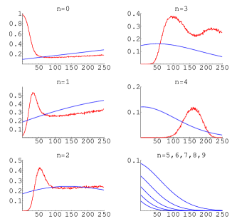
Figure 3: The red, wiggly curves show the probability that the $i$-th flux is $n$, $\tilde{p}_{i}(n)$, in the penultimate vacua of $N=7000$ decay chains starting from $\lambda\gtrsim 0.8$ in Model 1, as a function of $i$. For comparison, the blue, smooth curves show the probabilities that would have been obtained without cosmological selection, just from restricting to vacua with small cosmological constant. The differences are immediately apparent and quite drastic. For example, no fluxes greater than 4 survive the selection process; without selection, there would be many such fluxes. The fluxes associated with small charges (small $i$) are anomalously low after selection.

The probability distribution of fluxes characterizing the selected vacua becomes independent of the initial distribution for initial values of $\lambda\gtrsim 0.8$ (see Fig. 2). This asymptotic distribution is what we are after: it is the one picked out by the initial conditions chosen in Sec. II.4. To improve the statistical quality of our final data, we therefore merged the distributions obtained from initial $\langle\lambda\rangle=0.8,0.9,\ldots,1.4$, effectively obtaining $N=7000$ runs.

The resulting probability distribution of fluxes characterizing the selected vacua, $\tilde{p}_{i}(n)$, is shown as a function of $i$ in Fig. 3, and as a function of $n$ in Fig. 4. For comparison, we show the probabilities that would have been obtained from a random sample of vacua with comparable cosmological constant, without cosmological selection.

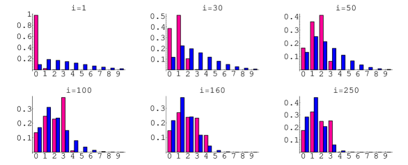
Figure 4: Specific examples of probability distributions $\tilde{p}_{i}(n)$, plotted against $n$ for 6 of the 250 fluxes in Model 1. The cosmological dynamics drives most fluxes into a narrower range (red/light shaded bars) than the distribution obtained from landscape statistics alone (blue/dark bars).

The overall strength of the selection effects (our first question in Sec. II.1) can be quantified by the ratio of selected vacua to the total number of vacua with distinct cosmological constant in the interval $0<\lambda<\lambda_{0}$ (the thin black shell in Fig. 1). We find from Eq. (17) that ${\cal N}_{\lambda_{0}}\approx 10^{80}$, so

$$\frac{{\cal N}_{\lambda_{0}}}{{\cal N}_{\lambda_{0}}^{\rm unselected}}\approx 10^{-41}~{}.$$ (20)

In other words, only one out of every $10^{41}$ vacua with small cosmological constant is actually accessed by cosmological selection.

After taking into account degeneracies, there remain effectively $\tilde{\cal N}_{\lambda_{0}}\approx 10^{22}$ distinct values of $\lambda$ that are accessed by cosmological selection. Hence, the cosmological constant problem can still be solved in this model, albeit with a much reduced discretuum density.

In order to answer the second question posed in Sec. II.1, let us inspect the probability distributions $\tilde{p}_{i}(n)$ in more detail, and look for characteristics that distinguish the selected vacua from the full set of vacua with small cosmological constant. In principle, every one of the $J$ fluxes will have a different probability distribution, leading to $O(J)$ predictions. For example, the first flux $n_{1}$ vanishes with $95\%$ probability. Before selection, by constrast, it would have been unlikely to do so ($10\%$; see the first panel in Fig. 4).

Instead of going through each flux, it is more illuminating to identify general trends, paying special attention to features that would have been extremely unlikely in the unselected sample. Quite clearly, small charges tend to have smaller fluxes. Interestingly, this is precisely the opposite of what would be naively expected without cosmological dynamics.

Let us define $i_{\rm max}(n)$ to be the largest $i$ such that there is less than $1\%$ chance to find one or more $n_{j}>n$ in the range $1\leq j\leq i$. For the selected vacua, we have $i_{\rm max}(1)=14$, $i_{\rm max}(2)=31$ and $i_{\rm max}(3)=77$. Without cosmological selection, by contrast, it is practically certain that one or more fluxes in the above ranges will exceed $n$.

Strictly speaking, we cannot resolve probabilities less than $N^{-1}$, the limit from the number of Monte Carlo runs. However, one would expect to obtain much stronger predictions by involving analytic arguments. For example, the $p_{i}(4)$ graph shows that for each $i<34$, the probability of finding $n_{i}=4$ is “zero”, i.e., less than $N^{-1}$. Dynamically, this must have resulted from a strong preference for such fluxes to decay—a preference that must have been present over more than $34$ steps in the decay chain. For example, if we assume that $n_{1}=4$ at some point in the decay chain, it must be true that long before the end of the decay chain, the probability for it to remain untouched must become very small. But then it will be small for each of the remaining steps. Hence, we expect that $p_{1}(4)$ is not just less than $N^{-1}$, but in fact exponentially small.

We have studied a range of other model parameters to ensure that our results are not peculiar features of this model. For example, in Model 2 with $J=200$, $\lambda_{\rm bare}=-0.6$, and $q_{i}=0.01494+0.03\frac{i}{J}$, we find $\frac{{\cal N}_{\lambda_{0}}}{{\cal N}_{\lambda_{0}}^{\rm unselected}}\approx 10^{-23}$; the selection effect is smaller but still considerable. The number of different values of $\lambda\sim\lambda_{0}$ is $\tilde{\cal N}_{\lambda_{0}}^{\rm unselected}\approx 10^{39}$ before cosmological selection and $\tilde{\cal N}_{\lambda_{0}}\approx 10^{16}$ after selection. Thus, as in the previous model, cosmological selection effects yield predictions but keep the model viable.

Of course, there will also be models which are ruled out by cosmological selection effects. The simplest way to find such models is to reduce the discretuum density before selection, for example by reducing the number $J$ of fluxes or decreasing $|\lambda_{\rm bare}|$. If the model contains only a few vacua with $\lambda\sim\lambda_{0}$ to start with, chances are that there will be none left after cosmological selection effects are taken into account. For example, consider Model 3 with $q_{i}=0.01494+0.03\frac{i}{J}$, $J=200$ and $\lambda_{\rm bare}=-0.4$. The discretuum density per $\lambda_{0}$ is $\tilde{\cal N}_{\lambda_{0}}^{\rm unselected}\approx 10^{24}$ before selection but $\tilde{\cal N}_{\lambda_{0}}\approx 10^{-12}$ after selection. In other words, not even a single vacuum with $\lambda\sim\lambda_{0}$ can be accessed. This model is ruled out by cosmological selection.

But the strength of selection effects can also vary. For example, Model 4 with $q_{i}=0.01494+0.03\frac{i}{J}$, $J=150$, $\lambda_{\rm bare}=-1.0$ has the same $\tilde{\cal N}_{\lambda_{0}}^{\rm unselected}\approx 10^{24}$ as Model 3. But after cosmological selection, the discretuum density per $\lambda_{0}$ is $\tilde{\cal N}_{\lambda_{0}}=10^{13}$, still larger than $1$, so the model remains viable.

Finally, we should mention that there can also be models in which cosmological selection effects are unimportant. For example, for very small charges $q_{i}\ll 1$, the typical fluxes $n_{i}$ will be large, and their standard deviations $\delta n_{i}$ in the interval $0<\lambda\leq\lambda_{0}$ can be much larger than the typical enhancement or suppression of fluxes by cosmological selection effects. However, such models appear unnatural in the context of string theory. Hence, we expect that the true string theory landscape will exhibit nontrivial cosmological selection effects.

IV Discussion

We can understand the selection behavior qualitatively by studying the tunneling rates, $e^{-B}$, where $B(q_{i},n_{i})$ is the instanton action given in Eq. (II.2). Let us neglect tunneling events that increase the magnitude of a flux $n_{i}$. Then $\partial B/\partial n<0$. This means that among two unequal fluxes with similar charge ($q_{i}\approx q_{j}$), the larger flux, $\max\{|n_{i}|,|n_{j}|\}$, is more likely to decay. The dependence on the size of the charge is more complicated. For most of the parameter space explored here, one finds $\partial B/\partial q>0$, which implies that among two equal fluxes $|n_{i}|=|n_{j}|$, the flux associated with the smaller charge, $\min\{q_{i},q_{j}\}$, is more likely to decay. (Exceptions can occur in the final stages of the decay process.)

Figure 5: Constant action surfaces for $\lambda=0.8$ (top-left), $\lambda=0.4$ (top-right), $\lambda=0.2$ (bottom-left), and $\lambda=0.1$ (bottom-right) in the $i$-$|n_{i}|$ plane. (Recall that the charges $q_{i}$ are ordered so as to increase monotonically with $i$.) The action $B$ grows towards the bottom right with a line spacing of $1$ in all four plots, corresponding to greater suppression of the decay.

In order to understand how these effects combine and compete, we have plotted the lines of constant action in the flux-charge plane, for a number of values of the cosmological constant $\lambda$, in Fig. 5. At the beginning of the decay chain, for large $\lambda$, the action ranges only over an interval of a few, so the most unlikely decay and the most likely decay do not differ enormously in probability. In this regime, our simulation shows that even upward jumps (which are neglected in Fig. 5) are not very suppressed.

As $\lambda$ decreases below $0.8$, a preference for the decay of fluxes with small $q_{i}$ and/or large $|n_{i}|$ becomes apparent. The slope of the constant action lines indicates how these tendencies are balanced. Starting around $\lambda=0.2$, the elimination of large fluxes is strongly preferred. This explains the absence of fluxes $|n_{i}|\geq 5$ in our results (see Fig. 3, last panel). In their absence, the last panel of Fig. 5 shows a strong preference for the decay of the fluxes associated with the smallest few charges. At least qualitatively, this explains the peaks in the first few panels in Fig. 3.

Throughout the decay, in all four panels of Fig. 5, the decay of fluxes with both small $|n_{i}|$ and large $q_{i}$ is relatively suppressed. This suggests that such fluxes will be left untouched by the cosmological dynamics, and instead will be set by initial conditions. To check this conclusion, let us compare the probability distribution $\tilde{p}_{i}(n)$ obtained from the $N$ penultimate vacua, with the distribution at the beginning of the decay chain. This is shown in Fig. 6. The first three panels ($n\leq 2$) demonstrate that the initial probabilities are indeed preserved for sufficiently large $i$.

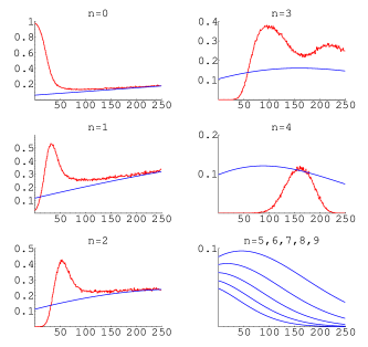
Figure 6: The red, wiggly curves are the same as in Fig. 3. The blue, smooth curves show the probabilities for various flux values near the beginning of the decay chain, at $\lambda=0.8$. In the first few panels, it is apparent that small fluxes associated with large charges do not participate in the dynamics. This can be understood from the functional form of the instanton action.

V Comparison with an alternative measure

We have computed the probability distribution $\tilde{p}_{i}(n)$ from the measure proposed in Ref. Bou06 . Other cosmological measures have been proposed, and it is important to ask which, if any, of the proposals is on the right track. In our view, this problem should be treated no differently from any other challenge to come up with the right theory describing a set of phenomena. The measure problem, like the question of the dynamical laws governing the early universe, is an aspect of the theoretical challenge faced in quantum cosmology. It should be approached by a combination of seeking out simple guiding principles (such as the causal-diamond viewpoint of the universe that leads to the holographic measure used here), and elimination. If a measure, or a theory, is poorly motivated, then it is unlikely to get much attention; and if a theory with a given measure yields absurd predictions, then the theory or the measure or both must be wrong.

An interesting proposal which has been quite sharply formulated is the measure of Garriga, Schwartz-Perlov, Vilenkin, and Winitzki GarSch05 (GSVW). This measure has been applied to a simplified BP model by Schwartz-Perlov and Vilenkin SchVil06 (SV), so let us compare results.

V.1 Initial conditions and computational complexity

Before going into the details, we note some formal differences. The GSVW measure depends on initial conditions only through the sign of the initial cosmological constant. We know of no fundamental reason why cosmological dynamics should be required to have this property. It would be nice if we were spared the task of understanding the initial conditions. But even in the GSVW measure one would still need to understand why the universe started in a de Sitter vacuum.

The measure we have used depends on initial conditions in additional ways, for example through the value of the initial cosmological constant. As we have seen, however, the dependence is weak if we assume that it enters mainly through $\lambda$. But clearly, initial conditions remain an free variable when applying the holographic measure; we have argued only that within a wide range that appears to be physically reasonable, the measure is not very sensitive to them.

It is unclear whether in practice, the GSVW measure can actually be applied to a rich landscape such as that of string theory, as we have done here for the holographic measure. As shown in Ref. SchVil06 , the GSVW probability distribution is dominated by the offspring of the longest-lived metastable vacuum. This requires finding the eigenvector $\mathbf{s}$ with smallest-magnitude negative eigenvalue of a matrix with rank ten to the hundreds. Perhaps statistical methods can be developed for this purpose, but so far the problem is unsolved. It is harder than the problem we addressed here of statistically solving Eq. (1), and it may be computationally intractible in a realistic landscape, in the sense of Ref. DenDou06 .

In any case, SV considered only a toy-BP-model with $J=7$ charges and a few million vacua. Then the eigenvector $\mathbf{s}$ can be found perturbatively in the small upward tunneling rates. Because of the much smaller number of vacua (in particular, their model does not contain any vacua with $\lambda\sim\lambda_{0}$), we cannot directly compare the results of SV to our results for a landscape with $\sim 10^{250}$ vacua.

Even at a qualitative level, Ref. SchVil06 contains no predictions of likely flux distributions that could be compared to ours. However, there is one robust prediction of the GSVW measure, which is not shared by the holographic measure, and which appears to conflict with observation. We turn to this problem next.

V.2 The staggering problem

The most important feature in the results of SV is the “staggered” nature of the probability distribution. The GSVW probabilities are widely spread. At first order in the perturbative approximation pursued by SV, the logarithmic range of probabilities, $\log\tilde{p}_{A}$, appears to be larger than the number of vacua. (A similar conclusion was reached in Ref. Sch06 for a different landscape.)

This behavior is in sharp contrast to our distribution, and it is extremely problematic. As SV point out, if the staggered behavior persisted at all orders in the full string landscape, the cosmological constant problem could no longer be solved. Then either the landscape or the GSVW measure would be ruled out. At first order in the SV approximation, staggering is generic, but one might hope that at higher order, a more uniform probability distribution will emerge Sch06 .

However, we will argue that staggering is a very general feature of the GSVW measure. We will use a result proven in Appendix C: The GSVW measure can be perfectly mimicked by the holographic measure, if the initial state $\mathbf{P}^{(0)}$ is chosen to be the GSVW eigenvector $\mathbf{s}$, which is dominated by the longest-lived metastable vacuum in the landscape, $(*)$. This result allows us to estimate the Shannon entropy of the GSVW probability distribution by following the branching trees of Ref. Bou06 .

Unlike in the earlier sections, we will be estimating the probability of vacua directly, not as a product of probabilities of individual fluxes. The Shannon entropy is then given by

$$S_{\rm GSVW}=-\sum_{A}\tilde{p}_{A}\log\tilde{p}_{A}~{},$$ (21)

and the effective number of selected vacua is ${\cal N}_{\rm GSVW}=\exp(S_{\rm GSVW})$. The cosmological constant problem can only be solved if ${\cal N}_{\rm GSVW}\gg 10^{120}$. In a staggered probability distribution, the most likely few vacua dominate the probability and the entropy, so $S_{\rm GSVW}\sim O(1)$, which is far too small. We will now argue that this type of distribution results from the GSVW measure quite generally.

As SV point out, the $(*)$ vacuum, by virtue of being long-lived, will have a relatively small cosmological constant, and upward tunneling will be enormously suppressed. Let us denote by $\epsilon$ the total branching ratio for upward tunneling. By Eq. (II.2), $\log\epsilon\sim-1/\lambda_{*}$, where $\lambda_{*}$ is the cosmological constant of the $(*)$ vacuum, so that $-\log\epsilon\gg 1$. After one upward tunneling, the cosmological constant is larger, but still only of order $\langle n_{i}\rangle q_{i}^{2}\sim O(q_{i}/\sqrt{J})$, which is less than $10^{-2}$ in natural models, so upward tunneling remains extremely suppressed. Following SV, let us thus use upward tunneling as a small expansion parameter. At zeroth order, we consider only downward tunneling.

SV showed that the eigenvector $\mathbf{s}$ is dominated by one component, the $(*)$ vacuum, and that the $(*)$ vacuum will have a small enough cosmological constant to access only terminal vacua by a single downward decay. The arguments leading to this conclusion generalize to realistic models. However, to show that the GSVW entropy is small, we will only rely on the weaker statement that the GSVW-equivalent initial conditions correspond to starting from a small number of initial vacua whose downward decay leads to terminal vacua after very few steps.

Let us imagine that the downward decay of any metastable vacuum affects each flux with equal relative probability, $1/J$. Moreover, let us pretend that decay chains never merge; all vacua reached by downward decays are different. These assumptions vastly overestimate the spread of probabilities and thus overestimate the GSVW entropy, for two reasons. First, we are at small cosmological constant and some decay channels will be much more suppressed than others; vanishing fluxes cannot decay downward at all. Second, the effective number of selected vacua will also be smaller since some vacua will be reached by more than one decay chain.

For simplicity, we assume that the tree contains only metastable vacua until the $D$-th step, at which point all vacua will be terminal. Starting from the the $(*)$ vacuum, $D$ will most likely be 1, but when starting a downward progression after the first upward jump, $D$ can be a few, so let us keep it general.

At zeroth order, we thus have $D$ generations of vacua. The $d$-th generation contains $J^{d}$ vacua with normalized probability $p_{d,0}\sim 1/DJ^{d}$ (the second index refers to the zeroth order). A bound on the zeroth order entropy is therefore

$$S_{\rm GSVW,0}<-\frac{1}{D}\sum_{d=1}^{D}\log\frac{1}{DJ^{d}}=\log D+\frac{D+1}{2}\log J~{},$$ (22)

This is of order one for realistic values of $J\lesssim O(1000)$ and $D\sim O(1)$.

The number of states, ${\cal N}_{\rm GSVW,0}\sim DJ^{\frac{D+1}{2}}$, is very small compared to $10^{120}$—far too small to include vacua with $\lambda\sim\lambda_{0}$. Typically, anthropic considerations cannot help in such a case, since most observers will be rare fluctuations in a vacuum with $\lambda\gg\lambda_{0}$. Hence, the GSVW measure is not capable of populating the landscape at leading order.

Before turning to higher order corrections, let us pause to ask whether the holographic measure would have succeeded at this stage, i.e., “at leading order”, when upward tunneling is neglected. Indeed, our simulation obtains large entropy even if upward tunneling is turned off. However, one might be concerned that this is mainly the result of starting from a large ensemble of vacua with similar, large $\lambda$, rather than just a single vacuum (natural though such a starting distribution may be Vil02 ).

But in fact the holographic measure would produce large $S$ even if we restricted $\mathbf{P}^{(0)}$ to a single member of the initial ensemble. The only thing that matters is that we start from a generic initial vacuum, for which $\lambda$ is of order unity. Then there will be a large number $D\sim O(\sqrt{J}/q)$ of downward tunnelings ($D\sim O(100)$ in our model) before the cascade terminates, and Eq. (22) yields ${\cal N}\sim J^{O(\sqrt{J}/q)}$, which is much larger than $10^{120}$ in generic models.

Returning to the GSVW measure, the entropy in Eq. (22) receives corrections at higher order. We will now argue that they are suppressed by powers of $\epsilon\ll 1$ and so they will hardly change the zeroth order entropy. In particular, they will not change the conclusion that ${\cal N}_{\rm GSVW}\ll 10^{120}$.

At each order, we make one upward jump and gain one “supergeneration”, or downward cascade of vacua, to which the above analysis can again be applied. Because upward tunneling is so highly suppressed, it will almost certainly originate from the largest-$\lambda$ vacuum in the $u$-th supergeneration and lead to a strongly preferred vacuum with larger $\lambda$. Corrections to this assumption will be considered below.

Then the GSVW entropy may again be (over-)estimated by the normalized probability distribution

$$p(u,d)=\frac{1-\epsilon}{D}\frac{\epsilon^{u}}{J^{d}}~{},$$ (23)

for a vacuum in the $d$-th generation of the $u$-th supergeneration. Thus the GSVW entropy is bounded by

$$S_{\rm GSVW} < \sum_{u=0}^{\infty}\sum_{d=0}^{D}p(u,d)$$

$$\approx \log\frac{D}{1-\epsilon}+\frac{\epsilon}{1-\epsilon}\log\frac{1}{\epsilon}+\frac{D+1}{2}\log J~{}.$$

This differs from the zeroth order result mainly through the negligible term

$$\epsilon\log\frac{1}{\epsilon}\ll 1~{},$$ (25)

so the GSVW entropy remains too small even at higher order.

We have neglected the $u$-dependence of both $\epsilon\ll 1$ and $D$. Choosing an upper bound $\epsilon\ll 1$ for all upward tunnelings and $D\lesssim O(1)$ for the number of downward generations will only overestimate the entropy but leave the conclusion unchanged. But at very high order, $u\sim O(\sqrt{J}/q)$, $\epsilon$ might be come $O(1)$, $D$ will become larger, and the expansion might break down. Can this change our conclusion?

To see that it will not, let us stop at $u$ of order a few, so that our approximations hold up to this point. Let us estimate the remaining contributions to the entropy by imagining that at this point the remaining probability flows equally into all vacua in the landscape, resulting in ${\cal N}$ vacua with probability $\epsilon^{u}/{\cal N}$. (This is almost certainly a large overestimate unless the landscape has no sinks or is extended far beyond the semiclassical regime.) But this contributes only of order

$$\epsilon^{u}\log\frac{\cal N}{\epsilon^{u}}$$ (26)

to the GSVW entropy. In a realistic landscape, we may safely assume that $\log{\cal N}\ll\epsilon^{-u}$ even for $u\sim O(1)$. Hence this contribution is also negligible.

We conclude that the GSVW entropy is dominated by the zeroth order term, Eq. (22). Its small size indicates that staggering is a general problem for the GSVW measure. It arises because the GSVW measure, in effect, attempts to populate the landscape starting from the longest-lived metastable vacuum. This fails since it relies on decay channels of enormously small relative probability. With reasonable initial conditions (such as starting with a randomly chosen vacuum or an ensemble at large $\lambda$), this problem is absent in the holographic measure.

Appendix A Statistical independence of fluxes

Let us discuss the assumption that the $J$ fluxes are statistically independent. We will argue that there is some minor interdependence because $J$ is finite, and we will explain how we correct for the corresponding constraint. Since the correction is small, some readers may wish to skip this appendix.

If there are correlations between the distributions $p_{i}(n)$, then their entropies do not simply add. In this case, the total number of states will be lower than the “maximum randomness” formula, Eq. (12), would make us believe. This will not be a concern for our sample of $N$ initial vacua, nor for our unbiased samples of vacua with small cosmological constant (without including selection effects from cosmological dynamics). As we discuss in Appendix B below, one can generate suitable samples by treating the fluxes as statistically independent. However, it is a concern for the $N$ vacua we arrive at by selection though a Monte Carlo chain.

In fact, an obvious correlation is introduced by our choice to consider the penultimate vacuum in each chain. By construction, these vacua must have a positive cosmological constant small enough that the next flux decay can make $\lambda$ negative. Thus, they satisfy the constraint

$$2|\lambda_{\rm bare}|\leq\sum_{i}n_{i}^{2}q_{i}^{2}<2|\lambda_{\rm bare}|+(2n_{j}-1)q_{j}^{2}$$ (27)

for at least one flux $j$. This constraint would be unimportant if $J$ was very large, but in realistic models, $J$ is only of order a few hundred.

The number of vacua with distinct vacuum energies of order $\lambda_{0}$ was estimated in Eq. (17). The correction due to the constraint (27) can be approximately implemented as follows. The entropy of the unconstrained ensemble is larger than the true entropy, with the extra states coming from vacua that fail to satisfy Eq. (27). But consider the distribution of vacua over the cosmological constant, $d\tilde{\cal N}/d\lambda$, in both the constrained and unconstrained ensembles. In the range of $\lambda$ where Eq. (27) is guaranteed to hold (which ranges from $\lambda=0$ to an upper bound much larger than $\lambda_{0}$), the two distributions $d\tilde{\cal N}/d\lambda$ will agree well.

From this viewpoint, the problem with Eq. (17) is not that $\tilde{\cal N}$ is computed from the unconstrained ensemble; the problem is that $dN/d\lambda$ is not. But this is easy to correct. Let us keep only the probabilities $\tilde{p}_{i}(n)$ obtained from the Monte Carlo chain, but replace the actual sample of $N$ vacua satisfying the constraint with a broader sample of $N^{\prime}$ vacua randomly generated from the $\tilde{p}_{i}(n)$, with the $\tilde{p}_{i}(n)$ treated as truly independent. This will spread the vacua over a larger range of $\lambda$ and thus reduce the number of vacua with $\lambda\sim\lambda_{0}$:

$$\tilde{\cal N}_{\lambda_{0}}=\lambda_{0}\left.\frac{d\tilde{\cal N}}{d\lambda}\right|_{\lambda=0}\approx\lambda_{0}\frac{\tilde{\cal N}}{N^{\prime}}\left.\frac{dN^{\prime}}{d\lambda}\right|_{\lambda=0}~{},$$ (28)

In the models studied in this paper, this correction reduces the number of vacua with $\lambda\sim\lambda_{0}$ by about one order of magnitude.

In principle, additional correlations could arise through the dynamics. By Eq. (II.2), however, the decay rate of each flux depends on the other fluxes only through $\lambda$ (and not, for example, though terms like $(n_{i}-n_{i+1})^{2}$, which could introduce clustering). The vast majority of possible flux combinations at each step in decay chains starting from a fixed value of $\lambda$ are mapped to a small range of $\lambda$, so the relative decay rates determining the next step cannot be sensitive to the detailed distribution of fluxes.

A very conservative upper bound on such correlations can be obtained by ignoring averaging. Instead, let us imagine that decay chains fall into two families, one of which has higher values of $\lambda$ at each step. But they cannot differ by more than the amount by which the final decay, at the end of the chain, changes $\lambda$ (or else, the steps can just be relabeled so as to match the families more closely). At the beginning of the chain, the decay is random for either family, since $\lambda$ is large. So the two families can differ at most by the effect of one additional decay at the end. Thus, we can bound dynamical correlation effects by comparing our sample of penultimate vacua with the ultimate vacua they decay to. But in the models we study, the corresponding probability distributions, $p_{i}(n)$, barely differ.

Appendix B Generating an unbiased sample

Consider all the vacua whose cosmological constant lies in a small interval $\delta\lambda$ around some value $\lambda$. On a number of occasions in this paper, we require an unbiased sample of such vacua. This task is equivalent to throwing all the vacua in the interval $\delta\lambda$ into a bag, pulling one out, returning it, and repeating this process $\hat{N}$ times to get a sample of size $\hat{N}$.

But the vacua are not in a bag; they are arranged in a grid on which the above interval corresponds to a spherical shell (see Fig. 1). Because the grid has a high dimension $J$, we must be careful to avoid directional effects that tend to pick vacua from preferred patches of the shell.

To generate a sample, we first need a set of probability distributions for the fluxes, $p_{i}(n)$. Vacua can be generated by picking the fluxes $n_{i}$ randomly according to the distributions $p_{i}(n)$. It is not necessary that all vacua thus generated lie in the interval $\delta\lambda$. We can reject those that do not, and generate vacua until we have $\hat{N}$ that do.

However, this procedure will generate directional bias if the ensemble of vacua defined by the $p_{i}(n)$ is not distributed spherically symmetrically in flux space. For example, if we specified that $p_{i}(n)$ is identical for all $i$, then the distribution would not be spherically symmetric since fluxes with large charge $q_{i}$ will tend to contribute more to the cosmological constant.

A spherically symmetric ensemble can be generated as a kind of canonical ensemble. Let us define a “temperature”, $T=1/\beta$, dual to the cosmological constant $\lambda$. Each flux contributes an “energy” $n_{i}^{2}q_{i}^{2}/2$, so its partition function is

$$z_{i}(\beta)=\sum_{n_{i}=-\infty}^{\infty}\exp\left(-\beta\frac{n_{i}^{2}q_{i}^{2}}{2}\right)~{}.$$ (29)

Treating the fluxes as independent, we obtain a total partition function

$$Z(\beta)=\prod_{i=1}^{J}z_{i}(\beta)=\sum_{n_{1},\ldots,n_{J}}e^{-\beta\Delta\lambda}~{},$$ (30)

where

$$\Delta\lambda(n_{1},\ldots,n_{J})\equiv\sum_{i=1}^{J}\frac{n_{i}^{2}q_{i}^{2}}{2}~{}.$$ (31)

Recall that $\lambda=-|\lambda_{\rm bare}|+\Delta\lambda$ by Eq. (5). Since the probability for each vacuum, $Z^{-1}e^{-\beta\Delta\lambda}$, depends on the fluxes only through the cosmological constant, the ensemble is manifestly direction-independent.

The individual partition functions, $z_{i}$, can be evaluated analytically for $\beta q_{i}^{2}/2\ll 1$:

$$z_{i}(\beta)\approx q_{i}^{-1}\sqrt{\frac{2\pi}{\beta}}~{},$$ (32)

and the expectation value of the “energy” $\Delta\lambda$ is given by

$$\langle\Delta\lambda\rangle(\beta)=\frac{J}{2\beta}~{}.$$ (33)

In order to generate a sample containing vacua near $\lambda$, we choose

$$\beta=\frac{J}{2(\lambda+|\lambda_{\rm bare}|)}~{},$$ (34)

and pick the fluxes $n_{i}$ randomly according to the probability distributions

$$p_{i}(n)=z_{i}^{-1}\exp\left(-\beta\frac{n^{2}q_{i}^{2}}{2}\right)~{}.$$ (35)

In this paper we have two distinct occasions to apply this method. The first is the task of generating initial vacua for our Monte Carlo chains. For a given initial $\lambda$ we generate $N=1000$ initial vacua according to Eqs. (34) and (35). From them, we generate $1000$ decay chains and inspect the final probability distribution $p_{i}(n)$ obtained from the penultimate vacua on the chains. We increase the initial $\lambda$ and repeat the process until the final distribution shows asymptotic behavior, i.e., until an increase in the initial cosmological constant no longer modifies our result.

The second application arises in estimating how many vacua with $0<\lambda\leq\lambda_{0}$ are present in a given BP model, before cosmological selection is taken into account. We will begin by discussing why the estimate given in Ref. BP is too crude in the present context.

By Eq. (5), vacua with small cosmological constant $0<\lambda\leq\lambda_{0}$ lie in a thin shell of radius

$$r=|2\lambda_{\rm bare}|^{1/2}$$ (36)

and width

$$\Delta r=\lambda_{0}/|2\lambda_{\rm bare}|^{1/2}$$ (37)

in flux space. Its volume is $\omega_{J-1}r^{J-1}\Delta r$, where $\omega_{J-1}=2\pi^{J/2}/\Gamma(J/2)$ is the area of a unit $J-1$ sphere.

In the limit where $r^{2}\gg\sum q_{i}^{2}$, directional effects in the lattice can be neglected, and the number of vacua in the shell can be estimated by comparing the volume of the shell to the volume of a single cell in the grid, $\prod_{i=1}^{J}q_{i}$ BP . In the same limit, the expectation values of the fluxes, $\langle n_{i}\rangle$, will be much larger than unity. Under the stronger condition that $r^{2}\gg(\sum q_{i})^{2}J$, the probability that at least one flux vanishes is very small. Then most values of $\lambda$ in the interval will be $2^{J}$-fold degenerate, and the number of different values of $\lambda$ in the interval $0<\lambda<\lambda_{0}$ can be estimated as

$$\tilde{\cal N}_{\lambda_{0}}\approx\frac{|\pi\lambda_{\rm bare}/2|^{J/2}}{\Gamma\left(\frac{J}{2}\right)}\,\frac{1}{\prod_{i=1}^{J}q_{i}}\,\frac{\lambda_{0}}{\lambda_{\rm bare}}$$ (38)

However, here we will study models in which the shell radii of interest are of the same order of magnitude as the diagonal of a grid cell: $r^{2}\sim\sum q_{i}^{2}$. For the same reason, typical vacua on the shell will have many vanishing fluxes ($n_{i}=0$). The $\lambda$-degeneracy of typical vacua will vary but will be less than $2^{J}$. Hence, Eq. (38) is unreliable.

The canonical ensemble yields a better estimate. With $\beta$ chosen so that $\langle\Delta\lambda\rangle\approx|\lambda_{\rm bare}|$, we obtain a canonical ensemble characterized by the probability distributions (35). In order to account for degeneracies, we treat vacua with the same cosmological constant as identical. The corresponding probability distributions $\tilde{p}_{i}(n)$, with $n\geq 0$, can be computed from Eq. (15). The full number of vacua in this ensemble, $\tilde{\cal N}$ is given by Eq. (18). The number of vacua in the tiny interval $0<\lambda<\lambda_{0}$ is given by Eq. (17). The distribution $dN/d\lambda$ can be obtained by generating $N$ vacua randomly from $p_{i}(n)$ [or $\tilde{p}_{i}(n)$] and binning them suitably.

Appendix C GSVW-equivalent initial conditions

In this appendix we show that our measure reproduces the GSVW measure GarSch05 if the initial probability distribution in Eq. (1) is taken to be a particular eigenvector singled out by the GSVW analysis.

We should warn that this initial condition is a very unnatural choice from the viewpoint of the holographic measure, and our result should not be interpreted as an equivalence of the two measures in any natural, physical sense. Indeed, finding the appropriate eigenvector $\mathbf{s}$ is the most challenging task in applying the GSVW measure. We are in effect using a nontrivial intermediate result of the GSVW analysis as an initial condition for the holographic measure. But this unified viewpoint allows us to reduce the difference between measures to a difference in initial conditions. In Sec. V, we use this viewpoint to clarify both the origin of “staggering” problem in the GSVW measure, and its absence in our measure.

Let us briefly summmarize the GSVW measure. It is derived from the evolution of a “comoving volume fraction”,

$$\frac{df_{B}}{dt}=\sum_{A}(-\kappa_{AB}f_{B}+\kappa_{BA}f_{A})~{},$$ (39)

where $\kappa_{AB}$ is the rate per unit time for a worldline in vacuum $B$ to enter vacuum $A$ (we neglect factors of the Hubble parameter). Let us restrict our attention to non-terminal vacua ($\lambda>0$), from whose volume fraction the GSVW probability distribution is ultimately computed (see below). We may then rewrite the above equation using the fact that terminal vacua do not tunnel back:

$$\frac{df_{b}}{dt}=-\sum_{A}\kappa_{Ab}f_{b}+\sum_{a}\kappa_{ba}f_{a}~{},$$ (40)

where $a,b$ only run over non-terminal vacua.

In the presence of terminal vacua, the solution to Eq. (40) is of the form

$$f_{a}(t)=s^{(1)}_{a}e^{-k_{1}t}+s^{(2)}_{a}e^{-k_{2}t}+\ldots$$ (41)

where $0<k_{1}<k_{2}\cdots$ GarSch05 . The GSVW probability is defined to be proportional to the “bubble abundance” produced by the slowest decaying state, the vector $\mathbf{s}^{(1)}$:

$$p_{A}=\sum_{b}\kappa_{Ab}s_{b}^{(1)}$$ (42)

Since the subleading terms are irrelevant, we will drop the sub- and superscripts and write $\mathbf{s}\equiv\mathbf{s}^{(1)}$ and $k\equiv k_{1}$.

For simplicity, we first demonstrate the claimed equivalence for the probability of non-terminal vacua. Let us write the above equations in matrix form:

$$\frac{d\mathbf{f}}{dt}=(\mathbf{K}-\mathbf{J})\mathbf{f}~{},$$ (43)

where $J_{ab}=\delta_{ab}\sum_{A}\kappa_{Ab}$ is a diagonal matrix, and $\mathbf{K}$ is the matrix with components $\kappa_{ab}$. The eigenvector $\mathbf{s}$ satisfies

$$({\mathbf{K}-\mathbf{J}}){\mathbf{s}}=-k{\mathbf{s}}.$$ (44)

The unnormalized GSVW probabilities for non-terminal vacua are

$${\bf p=Ks}~{}.$$ (45)

By Eq. (2), the absolute decay rates are related to the branching ratios by

$${\bf EJ=K}~{},$$ (46)

where $\mathbf{E}$ is the matrix with components $\eta_{ab}$. Combining the above four equations, we obtain

$$(1-\mathbf{E}){\bf p} = (1-\mathbf{E}){\bf Ks}$$ (47)

$$= (1-\mathbf{E})({\bf J}-k){\bf s}$$

$$= ({\bf J-K}-k+k\mathbf{E}){\bf s}=k\mathbf{E}{\bf s}~{}.$$

Comparison with Eq. (1), with initial condition $\mathbf{P}^{(0)}=\mathbf{s}$, reveals that the GSVW probability agrees with the holographic probability up to an overall factor $k$ that will be absorbed by normalization:

$$\mathbf{p}\propto\mathbf{P}~{}~{}\mbox{for}~{}~{}~{}\mathbf{P}^{(0)}=\mathbf{s}~{}.$$ (48)

To include terminal vacua, we extend the above argument to vectors and matrices containing terminal components. A prime will denote the non-square matrix of decay rates from terminal into terminal vacua. First, we note that the GSVW probabilities are independent of any terminal components $\mathbf{s}^{\prime}$ ascribed to the eigenvector:

$$\mathbf{p}=\left(\begin{array}[]{cc}\mathbf{K}&0\\ \mathbf{K^{\prime}}&0\\ \end{array}\right)\left(\begin{array}[]{cc}\mathbf{s}\\ \mathbf{s}^{\prime}\\ \end{array}\right)=\left(\begin{array}[]{cc}(\mathbf{J}-k)\mathbf{s}\\ \mathbf{K^{\prime}s}\\ \end{array}\right)\\$$ (49)

Similarly, by Eq. (1), the holographic measure does not depend on the terminal components of the initial probability distribution $\mathbf{P}^{(0)}$. For convenience, we might as well set $\mathbf{s}^{\prime}=0$.

The remaining question is whether the (final) probabilities for terminal vacua agree. From Eq. (2) we have

$$\left(\begin{array}[]{cc}\mathbf{E}&0\\ \mathbf{E}^{\prime}&0\\ \end{array}\right)\left(\begin{array}[]{cc}\mathbf{J}&0\\ 0&0\\ \end{array}\right)=\left(\begin{array}[]{cc}\mathbf{E}\mathbf{J}&0\\ \mathbf{E}^{\prime}\mathbf{J}&0\\ \end{array}\right)=\left(\begin{array}[]{cc}\mathbf{K}&0\\ \mathbf{K^{\prime}}&0\\ \end{array}\right)~{},$$ (50)

so that

$$(1-\eta)\mathbf{p} = \left(\begin{array}[]{cc}1-\mathbf{E}&0\\ -\mathbf{E}^{\prime}&1\\ \end{array}\right)\left(\begin{array}[]{cc}(\mathbf{J}-k)\mathbf{s}\\ \mathbf{K^{\prime}s}\\ \end{array}\right)$$ (55)

$$= \left(\begin{array}[]{cc}(1-\mathbf{E})(\mathbf{J}-k)\mathbf{s}\\ \left[-\mathbf{E}^{\prime}(\mathbf{J}-k)+\mathbf{K^{\prime}}\right]\mathbf{s}\end{array}\right)$$ (58)

$$= \left(\begin{array}[]{cc}k\mathbf{E}\mathbf{s}\\ k\mathbf{E}^{\prime}\mathbf{s}\\ \end{array}\right)=k\left(\begin{array}[]{cc}\mathbf{E}&0\\ \mathbf{E}^{\prime}&0\\ \end{array}\right)\left(\begin{array}[]{cc}\mathbf{s}\\ \mathbf{0}\\ \end{array}\right)$$ (65)

$$= k\eta\mathbf{s}~{},$$ (66)

so Eq. (48) holds for both nonterminal and terminal components of the probability distribution.

Note that our result does not contradict a crucial difference between the GSVW measure and the holographic measure, namely that the former depends on absolute lifetimes of vacua whereas the latter knows nothing about them. (The former is constructed from the full matrix $\kappa$; the latter only from its normalized version, $\eta$.) To achieve equivalence, we had to impart the extra information contained in $\kappa$ to the holographic measure through a very special choice of initial condition, $\mathbf{s}$. We emphasize again that from the point of view of the latter measure, this choice would be completely unmotivated; the equivalence is useful mainly for clarifying the differences of the two measures (Sec. V).

References

- (1) R. Bousso, B. Freivogel and I.-S. Yang: Eternal inflation: The inside story. Phys. Rev. D 74, 103516 (2006), hep-th/0606114.
- (2) A. Linde, D. Linde and A. Mezhlumian: From the big bang theory to the theory of a stationary universe. Phys. Rev. D 49, 1783 (1994), gr-qc/9306035.
- (3) J. García-Bellido, A. Linde and D. Linde: Fluctuations of the gravitational constant in the inflationary Brans-Dicke cosmology. Phys. Rev. D 50, 730 (1994), astro-ph/9312039.
- (4) J. Garriga and A. Vilenkin: A prescription for probabilities in eternal inflation. Phys. Rev. D 64, 023507 (2001), gr-qc/0102090.
- (5) J. Garriga, D. Schwartz-Perlov, A. Vilenkin and S. Winitzki: Probabilities in the inflationary multiverse. JCAP 0601, 017 (2006), hep-th/0509184.
- (6) R. Easther, E. A. Lim and M. R. Martin: Counting pockets with world lines in eternal inflation (2005), astro-ph/0511233.
- (7) R. Bousso: Holographic probabilities in eternal inflation (2006), hep-th/0605263.
- (8) R. Bousso: Precision cosmology and the landscape (2006), hep-th/0610211.
- (9) L. Susskind, L. Thorlacius and J. Uglum: The stretched horizon and black hole complementarity. Phys. Rev. D 48, 3743 (1993), hep-th/9306069.
- (10) J. Preskill: Do black holes destroy information? (1992), hep-th/9209058.
- (11) R. Bousso, R. Harnik, G. D. Kribs and G. Perez: Predicting the cosmological constant from the causal entropic principle (2007), hep-th/0702115.
- (12) R. Bousso and J. Polchinski: Quantization of four-form fluxes and dynamical neutralization of the cosmological constant. JHEP 06, 006 (2000), hep-th/0004134.
- (13) D. Schwartz-Perlov and A. Vilenkin: Probabilities in the Bousso-Polchinski multiverse. JCAP 0606, 010 (2006), hep-th/0601162.
- (14) S. Weinberg: Anthropic bound on the cosmological constant. Phys. Rev. Lett. 59, 2607 (1987).
- (15) M. R. Douglas and S. Kachru: Flux compactification (2006), hep-th/0610102.
- (16) J. D. Brown and C. Teitelboim: Dynamical neutralization of the cosmological constant. Phys. Lett. B195, 177 (1987).
- (17) A. Vilenkin: Boundary conditions in quantum cosmology. Phys. Rev. D 33, 3560 (1986).
- (18) A. Linde: Quantum creation of an inflationary universe. Sov. Phys. JETP 60, 211 (1984).
- (19) F. Denef and M. R. Douglas: Computational complexity of the landscape. I (2006), hep-th/0602072.
- (20) D. Schwartz-Perlov: Probabilities in the Arkani-Hamed-Dimopolous-Kachru landscape (2006), hep-th/0611237.
- (21) A. Vilenkin: Quantum cosmology and eternal inflation (2002), gr-qc/0204061.