hep-th/0703197

UT-Komaba/07-2

TIT/HEP–569

TU–787

March, 2007

Statistical Mechanics of Vortices

from D-branes and T-duality

Minoru Eto¹, Toshiaki Fujimori², Muneto Nitta³,
Keisuke Ohashi², Kazutoshi Ohta⁴ and Norisuke Sakai²

¹University of Tokyo, Inst. of Physics Komaba 3-8-1, Meguro-ku Tokyo 153, JAPAN
²Department of Physics, Tokyo Institute of Technology
Tokyo 152-8551, JAPAN
³Department of Physics, Keio University, Hiyoshi, Yokohama, Kanagawa 223-8521, JAPAN
⁴Department of Physics, Graduate School of Science, Tohoku University
Sendai 980-8578, JAPAN

Abstract

We propose a novel and simple method to compute the partition function of statistical mechanics of local and semi-local BPS vortices in the Abelian-Higgs model and its non-Abelian extension on a torus. We use a D-brane realization of the vortices and T-duality relation to domain walls. We there use a special limit where domain walls reduce to gas of hard (soft) one-dimensional rods for Abelian (non-Abelian) cases. In the simpler cases of the Abelian-Higgs model on a torus, our results agree with exact results which are geometrically derived by an explicit integration over the moduli space of vortices. The equation of state for $U(N)$ gauge theory deviates from van der Waals one, and the second virial coefficient is proportional to $1/\sqrt{N}$, implying that non-Abelian vortices are “softer” than Abelian vortices. Vortices on a sphere are also briefly discussed.

1 Introduction

Knowledge of moduli space structure of solitons is important in order to understand not only their own dynamics but also non-perturbative effects in field theory. The moduli space structure of the solitons signifies its topology, metrics and singularities. The volume of the moduli space also possesses an important meaning and plays an essential role in understanding the non-perturbative dynamics. Recently Nekrasov has shown that the prepotential of ${\cal N}{=}2$ supersymmetric gauge theory in $d=3+1$ can be obtained from some statistical partition function, whose free energy measures the volume of the moduli space of Yang-Mills instantons [1]. The instanton moduli space is non-compact and of course the volume diverges, but a coefficient of the divergent part gives perturbative and non-perturbative information on supersymmetric gauge theory. It is also interesting that the partition function or the volume of the instantons is closely related to topological string amplitudes on suitable Calabi-Yau manifolds. Precisely speaking, the instantons, which are used for the calculation of the volume, are not solutions of the equations of motion in supersymmetric gauge theory. However, in the calculation of the partition function or the volume, the so-called localization theorem says that the result does not depend on details of the moduli space structure. This suggests that we do not need to know the exact solutions and metrics in order to calculate the volume of the moduli space of some class of BPS solitons. However, the issue has not been settled except for Yang-Mills instantons, since other examples and applications have not been investigated yet. For instance, similar method should be applicable to calculate the effective (super)potential of $d=1+1$ supersymmetric gauge theory from the statistical partition function associated with the volume of the vortex moduli space.

Another direct application of the volume of the moduli space is a classical statistical mechanics of the solitons. The Gibbs partition function of solitons at finite temperature $T$ is given by an integration over a phase space, which is a cotangent bundle $T^{*}{\cal M}$ of the moduli space $\cal M$ of solitons:

$$Z=\frac{1}{(2\pi)^{D}}\int_{T^{*}{\cal M}}d^{D}x\,d^{D}p\,e^{-H(\vec{x},\vec{p})/T}.$$ (1.1)

Here $D$ represents the dimensions of the moduli space, and $H(\vec{x},\vec{p})$ is a Hamiltonian of the soliton system in terms of the moduli parameters. If we assume that the solitons are sufficiently diluted and interactions can be ignored, we can regard the Hamiltonian as quadratic in momenta $H(\vec{x},\vec{p})=\frac{1}{2}g^{ij}(x)p_{i}p_{j}$ and $g^{ij}$ is the (inverse of) metric on ${\cal M}$. Then we can explicitly perform the integration over the momenta (cotangent direction). The partition function becomes

$$Z=\left(\frac{T}{2\pi}\right)^{D/2}\int_{\cal M}d^{D}x\,\sqrt{\det(g_{ij}(x))}=\left(\frac{T}{2\pi}\right)^{D/2}{\rm Vol}({\cal M}),$$ (1.2)

which is proportional to the volume of the moduli space [2]. Many applications and calculations from this point of view can be found [2]–[6] in the case of Abrikosov-Nielsen-Olesen (ANO) vortices [7], namely vortices in the Abelian-Higgs model at the critical coupling (the BPS limit).

On the other hand, non-Abelian BPS vortices have been recently found [8, 9] and extensively discussed in the (supersymmetric) non-Abelian Higgs model, which is the $U(N_{\rm C})$ gauge theory coupled with $N_{\rm F}(>N_{\rm C})$ fundamental Higgs fields. Like (non-commutative) instantons, single vortex in the $N_{\rm C}=N_{\rm F}$ case is found to carry internal moduli $\mathbb{C}P^{N_{\rm C}-1}$ in addition to position moduli. They can confine monopoles in the Higgs phase [10, 11] and this fact is applied [12, 13] to show coincidence of the BPS spectra of $d=3+1$, ${\cal N}=2$ supersymmetric gauge theory and $d=1+1$, ${\cal N}=2$ supersymmetric $\mathbb{C}P^{n}$ model. The moduli space of multiple ($k$-)vortices has been conjectured in string theory [8] and then has been completely determined in field theory [14, 15, 16], which has turned out to be some resolution of $k$-symmetric product of $\mathbb{C}\times\mathbb{C}P^{N_{\rm C}-1}$ [14]. Although its explicit metric is still unknown except for a single ($k=1$) vortex, an integration formula of the Kähler potential has been found [17]. The structure of the moduli space of two ($k=2$) vortices has been worked out [18, 16] and is applied to non-Abelian duality [19], and classical dynamics of non-Abelian vortex-strings has been clarified [20]. The extension to a superconformal field theory [21] as well as the Chern-Simons-Higgs theory [22] has been discussed.

In this article, we propose a novel and simple derivation of the volume of the moduli space of Abelian as well as non-Abelian (semi-)local vortices in order to apply to the statistical mechanics of vortex gas. We utilize a geometric and stringy (D-brane) interpretation of the Abelian and non-Abelian BPS vortices in supersymmetric gauge theory [8] and use a T-dual relation between the vortices and domain walls, which was proposed in [23, 24]. This interpretation shows us a schematic structure of the vortex moduli space without any detailed information on the exact solutions and metrics. (See Fig. 17 of Ref. [24] for the moduli space of two non-Abelian local vortices in $U(2)$ gauge theory.) It is interesting to observe that the T-duality reduces the calculation of the volume into a simple problem of a gas of hard rods between a one-dimensional interval in the Abelian case. The volume of the moduli space of the ANO vortices in the Abelian-Higgs model (with $N_{\rm C}=N_{\rm F}=1$) has been already calculated by [2]–[4] (see also §7 in [5]) and an analogy with the hard rod problem was pointed out there. However this relation has been mysterious for a long time. We can explain from a point of view of the T-duality in superstring theory why the one-dimensional hard rod problem appears. The advantage of our method is that it can be easily extended to the general cases, namely local and semi-local, Abelian and non-Abelian vortices. We find that the T-duality enables us to reduce the problem of a gas of non-Abelian local vortices to a gas of soft rods, in contrast to the hard rods in the case of Abelian local vortices. We obtain that the second virial coefficient is proportional to $1/\sqrt{N}$ for non-Abelian local vortices in $U(N)$ gauge theories at large $N$. This shows that the exclusion volume of a vortex behaves as $1/\sqrt{N}$ as we increases $N$, getting closer to an ideal gas. Moreover, equation of state for local vortices in $U(N)$ gauge theory deviates from van der Waals one, contrary to the case of the Abelian-Higgs model.

Comparing with the calculation in [2]–[5], our result in the Abelian case gives the precise answer even though we take a special limit to the configuration and do not use the exact metrics. So we expect that this is an another example where the localization theorem effectively works. In fact calculation of the volume of vortex moduli space using the localization theorem can be found in the case of the Abelian-Higgs model [6].

In Sec. 2 we give a brief review of brane configurations of vortices and domain walls. In sec. 3, we calculate the partition function of vortices in the Abelian-Higgs model, which agrees with the previous result. In sec. 4, we give general formula of the partition function of local/semi-local non-Abelian vortices which is new and shows the power of our method. We perform explicit calculation in several cases. Sec. 5 is devoted to a discussion. An interesting duality is observed and our method is extended to the case of a base manifold $S^{2}$. Appendix gives some details of derivation of the virial coefficient.

2 Non-Abelian Vortices and D-brane Interpretation

We first start with (2+1)-dimensional $U(N_{\rm C})$ gauge theory with $N_{\rm F}(\geq N_{\rm C})$ massless Higgs fields in the fundamental representation. The Lagrangian is given by

$$\mathcal{L}={\rm Tr}\left[-\frac{1}{2g^{2}}F_{MN}F^{MN}+\mathcal{D}_{M}H\left(\mathcal{D}^{M}H\right)^{\dagger}-\frac{g^{2}}{2}\left(HH^{\dagger}-c\mathbf{1}_{N_{\rm C}}\right)^{2}\right],$$ (2.1)

where $M,N$ are the indices of space-time $(M,N=0,1,2)$ and the space-time metric is chosen as $\eta_{MN}={\rm diag}(+1,-1,-1)$. The field strength is defined by $F_{MN}\equiv-i[\mathcal{D}_{M},\mathcal{D}_{N}]=\partial_{M}W_{N}-\partial_{N}W_{M}+i[W_{M},W_{N}]$, where $W_{M}$ is the $U(N_{\rm C})$ gauge field. The scaler fields $H^{rA}\,(r=1,\cdots,N_{\rm C}),\,(A=1,\cdots,N_{\rm F})$ are expressed by elements of an $N_{\rm C}\times N_{\rm F}$ matrix and the covariant derivative is defined by $\mathcal{D}_{M}H\equiv\partial_{M}H+iW_{M}H$. The constants $g$ and $c\,(>0)$ are the gauge coupling constant and the Fayet-Iliopoulos (FI) parameter respectively.

For static configurations, the energy is bounded from below as follows:

$$E = \int d^{2}x\,{\rm Tr}\left[\frac{1}{g^{2}}\left(F_{12}+\frac{g^{2}}{2}(c\mathbf{1}_{N_{\rm C}}-HH^{\dagger})\right)^{2}+\mathcal{D}_{\bar{z}}H\left(\mathcal{D}_{\bar{z}}H\right)^{\dagger}-cF_{12}\right]$$ (2.2)

$$\geq -c\int d^{2}x\,F_{12}=2\pi ck,$$

where the integer $k\equiv-\displaystyle\frac{1}{2\pi}\int d^{2}x\,F_{12}$ represents the number of vortices (vorticity). Since the configurations of the BPS vortices saturate the inequality Eq. (2.2), they satisfy the following BPS equations (the vortex equations):

$$\mathcal{D}_{\bar{z}}H=0,\hskip 28.45274ptF_{12}+\displaystyle\frac{g^{2}}{2}(c\mathbf{1}_{N_{\rm C}}-HH^{\dagger})=0.$$ (2.3)

If the fluctuation energy above the energy of the multi-vortex static configuration is less than that of the mass gap between massless moduli fluctuations and massive fluctuations, the dynamics of the system is well described by the geodesic motion on the moduli space $\mathcal{M}_{k}$ of the $k$ vortices (Manton’s moduli/geodesic approximation [25]), so that the Lagrangian for multi-vortex system is given by

$$L=g_{i\bar{j}}(\phi,\bar{\phi})\dot{\phi}^{i}\dot{\bar{\phi}}^{j},$$ (2.4)

where $\phi^{i},\bar{\phi}^{i},\left(~{}i=1,\cdots,D={\rm dim}_{\mathbb{C}}\,\mathcal{M}_{k}\right)$ are complex coordinates of the moduli space $\mathcal{M}_{k}$ and $g_{i\bar{j}}(\phi,\bar{\phi})$ is a Kähler metric of $\mathcal{M}_{k}$.

In the cases of compact base manifolds, there is the maximum number for vortices allowed to exist [26]. For general $N_{\rm C}$ with a torus $T^{2}$, this maximum number can be obtained by taking the trace of the second equation of the BPS equation (2.3) and by integrating over $T^{2}$ as

$$-2\pi k+N_{\rm C}\frac{g^{2}c}{2}A=\frac{g^{2}}{2}\int d^{2}x\,{\rm Tr}\left(HH^{\dagger}\right)\geq 0\quad\leftrightarrow\quad A\geq kB_{N_{\rm C}},$$ (2.5)

where $A$ is the area of the torus and we have defined the Bradlow area

$$B_{N_{\rm C}}\equiv\frac{1}{N_{\rm C}}{4\pi\over g^{2}c}.$$ (2.6)

The limit to saturate this inequality is called the Bradlow limit. In particular, we can regard $B_{1}={4\pi\over g^{2}c}$ as an effective area of the Abelian (ANO) vortex. Roughly speaking, the inequality (2.5) implies that we can squeeze as many vortices as $N_{\rm C}$ times the maximal number of the Abelian ($N_{\rm C}=1$) vortices for a given area $A$ of the torus. This behavior can be understood intuitively as due to the freedom for vortices to avoid occupying the same points in their additional internal moduli space $\mathbb{C}P^{N_{\rm C}-1}$ when they are squeezed too much in the actual configuration space. This freedom allows the non-Abelian vortices to overlap in the configuration space more easily compared to Abelian vortices. Therefore the effective area of the non-Abelian vortex $B_{N_{\rm C}}$ becomes $1/N_{\rm C}<1$ times the area of the Abelian vortices $B_{1}$. The Bradlow area $B_{N_{\rm C}}$ indicates the smallness of the effective area of vortices at the limiting high density of vortices. Note that there exists another inequality in the case of non-Abelian gauge theories with $N_{\rm C}>k$. Since all vortex solutions in this case can be embedded to a theory with a smaller number of colors $N_{\rm C}^{\prime}(=k^{\prime})=k$, the vortex configuration for $N_{\rm C}>k$ should satisfy the inequality for $N_{\rm C}^{\prime}=k$, that is,

$$A\geq{4\pi\over g^{2}c}~{}~{}(=B_{1})$$ (2.7)

stating that the area of the torus must be larger than that of one ANO vortex.

As we mentioned in Eq. (1.2), the classical partition function of $k$-vortex system is proportional to the volume of the moduli space $\mathcal{M}_{k}$.

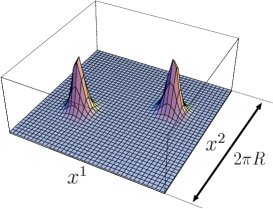
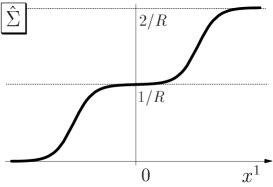
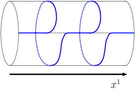
(a)	(b)	(c)

Fig. 1: Duality between vortices and domain walls: $N_{\rm C}=N_{\rm F}=1,~{}k=2$. (a) Profile of energy density of 2-vortex configuration on $\mathbb{R}\times S^{1}$ with period $2\pi R$, (b) Profile of $\hat{\Sigma}(x^{1})=-\frac{1}{2\pi R}\int dx^{2}W_{2}$, (c) Profile of $\hat{\Sigma}(x^{1})$ written on $\mathbb{R}\times S^{1}$ with period $1/R$.

To calculate this partition function (volume), we utilize the duality relation between vortices and domain walls [23, 24]. If we compactify $x^{2}$-direction on $S^{1}$ as $x^{2}\sim x^{2}+2\pi nR$, a vortex configuration can be viewed as domain walls. The profile of the kink solution of the domain walls is described by the eigenvalues of $\hat{\Sigma}$ defined by

$$\hat{\Sigma}(x^{1})=-\frac{1}{2\pi iR}\log\left[\mathbf{P}\exp\left(i\int_{0}^{2\pi R}dx^{2}\,W_{2}(x^{1},x^{2})\right)\right],$$ (2.8)

where $\mathbf{P}$ stands for the path-ordered product. Note that under the gauge transformation $U=e^{-inx^{2}/R}\mathbf{1}_{N_{\rm C}}$ ($n\in\mathbb{Z}$), $\hat{\Sigma}(x^{1})$ transforms as $\hat{\Sigma}\rightarrow\hat{\Sigma}+n/R\mathbf{1}_{N_{\rm C}}$ and there is an identification $\hat{\Sigma}\sim\hat{\Sigma}+n/R\mathbf{1}_{N_{\rm C}}$. Thus the eigenvalues of $\hat{\Sigma}(x^{1})$ are interpreted as a function which takes value in $S^{1}$ with radius $1/R$. Fig. 1 depicts an example of the $N_{\rm C}=N_{\rm F}=1$ case. The $k$-vortex configuration (Fig. 1-(a)) corresponds to the $k$-wall configuration (Fig. 1-(b)) in the fundamental region, and it also can be interpreted as the configuration of $\hat{\Sigma}(x^{1})$ with $k$ windings (Fig. 1-(c)) on the cylinder.

This duality can be regarded as a T-duality between the brane configurations of vortices [8] and domain walls [28]. Our model can be embedded into the supersymmetric system with eight supercharges and the associated model is realized by a combination of various kinds of branes in Type IIB superstring theory. The brane configurations are expressed in Table 1 and drawn in Fig.2 schematically.

	$x^{0}$	$x^{1}$	$x^{2}$	$x^{3}$	$x^{4}$	$x^{5}$	$x^{6}$	$x^{7}$	$x^{8}$	$x^{9}$
$N_{\rm C}$ $\rm D3$	$\bullet$	$\bullet$	$\bullet$	$\bullet$	$-$	$-$	$-$	$-$	$-$	$-$
$N_{\rm F}$ $\rm D5$	$\bullet$	$\bullet$	$\bullet$	$-$	$\bullet$	$\bullet$	$\bullet$	$-$	$-$	$-$
$2\hskip 5.69054pt{\rm NS}5$	$\bullet$	$\bullet$	$\bullet$	$-$	$-$	$-$	$-$	$\bullet$	$\bullet$	$\bullet$
$k\hskip 5.69054pt\rm D1$	$\bullet$	$\times$	$\times$	$-$	$\bullet$	$-$	$-$	$-$	$-$	$-$

(a) Brane configuration for vortices

	$x^{0}$	$x^{1}$	$x^{2}$	$x^{3}$	$x^{4}$	$x^{5}$	$x^{6}$	$x^{7}$	$x^{8}$	$x^{9}$
$N_{\rm C}$ $\rm D2$	$\bullet$	$\bullet$	$-$	$\bullet$	$-$	$-$	$-$	$-$	$-$	$-$
$N_{\rm F}$ $\rm D4$	$\bullet$	$\bullet$	$-$	$-$	$\bullet$	$\bullet$	$\bullet$	$-$	$-$	$-$
$2\hskip 5.69054pt{\rm NS}5$	$\bullet$	$\bullet$	$\bullet$	$-$	$-$	$-$	$-$	$\bullet$	$\bullet$	$\bullet$
$k\hskip 5.69054pt\rm D2^{\prime}$	$\bullet$	$\times$	$\bullet$	$-$	$\bullet$	$-$	$-$	$-$	$-$	$-$

(b) Brane configuration for domain walls

Table 1: Brane configurations for vortices and domain walls: Branes are extended along directions denoted by $\bullet$, and are not extended along directions denoted by $-$. The symbol $\times$ denotes the codimensions of the k D1-branes (D2’-brane) on the worldvolume of the D3-branes (D2-branes) excluding the $x^{3}$-direction which is a finite line segment.

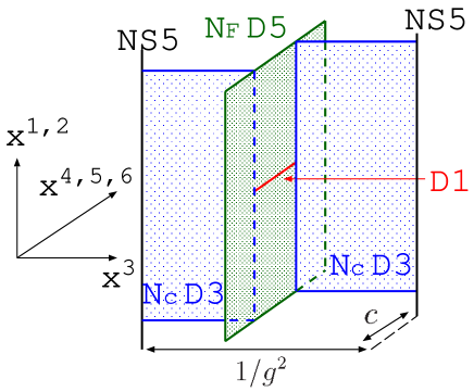
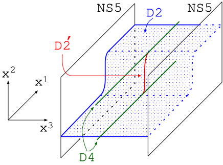
(a) Brane configuration for vortices	(b) Brane configuration for domain wall

Fig. 2: Brane configurations for vortices and domain wall

The $(2+1)$-dimensional $U(N_{\rm C})$ gauge theory coupled with $N_{\rm F}$ massless hypermultiplets is realized on $N_{\rm C}$ $\rm D3$ branes in the Hanany-Witten setup [29] as in Fig. 2-(a), since the $x^{3}$ direction of the $\rm D3$ brane worldvolume is a finite line segment. $\rm D1$ branes correspond to vortices in the $\rm D3$ brane worldvolume theory, since they are interpreted as codimension-two objects on the $\rm D3$ branes [8]. Fig. 2 shows the brane configuration T-dualized along the $x^{2}$-direction. The theory without vortices is mapped to the world-volume theory on the $N_{\rm C}$ D2 branes, which is the (1+1) dimensional $U(N_{\rm C})$ gauge theory with $N_{\rm F}$ (massive) hypermultiplets. The vortices are mapped to the kinky D2-branes representing domain walls [27, 28]. The eigenvalues of $\hat{\Sigma}(x^{1})$ can be interpreted as the position of D2 branes in $S^{1}$.

3 A Limit of the Profile and the Moduli Integration: the Abeain-Higgs Model

If we use the T-dual relation via the brane configuration, the evaluation of the volume of the vortex moduli space reduces to a calculation of the volume of the domain wall configurations (kink profiles). However, it is difficult to solve the domain wall equations and to integrate over their configuration space in general.

In order to proceed the evaluation, we demand an approximation which simplifies the profile of the domain wall solution. Now, let us consider a special limit

$$g^{2}c,\;1/R\rightarrow\infty,\quad\text{with}\quad d\equiv\frac{2}{g^{2}cR}:\mbox{ fixed}.$$ (3.1)

Of course, this is a rough approximation with respect to the kink profile, we will amazingly find that we can obtain the exact results even in this limit. Note that using $d$ defined above the inequalities (2.5) and (2.7) are translated in the T-dualized picture to

$$2\pi R^{\prime}\geq\frac{1}{N_{\rm C}}kd\ ,\qquad 2\pi R^{\prime}\geq d,$$ (3.2)

respectively. These inequalities can be easily shown even in this T-dualized picture as dicussed below. This fact is the first evidence for the usefulness of our T-dualized picture in this paper.

Here we describe a limit shape of the ANO vortices in the Abelian-Higgs model ($N_{\rm C}=N_{\rm F}=1$) for simplicity. In this case, the moduli space of the multi-vortex system consists of the position of each vortex. The positions of vortices in the $x^{2}$-direction are translated into the phase degrees of freedom of domain walls after the T-duality along $x^{2}$direction. If one vortex is located at $z=0$, the corresponding function $\hat{\Sigma}(x^{1})$ is given by

$$\hat{\Sigma}(x^{1})=\left\{\begin{array}[]{clc}0&\quad\text{for}&x^{1}<-\dfrac{d}{2}\\ \dfrac{1}{Rd}\left(x^{1}+\dfrac{d}{2}\right)&\quad\text{for}&-\dfrac{d}{2}<x^{1}<\dfrac{d}{2}\\ \dfrac{1}{R}&\quad\text{for}&x^{1}>\dfrac{d}{2}\end{array}\right..$$ (3.6)

From this expression, we find that the parameter $d$ represents the effective thickness of the dual domain wall. Fig. 3 shows the profiles of $\hat{\Sigma}(x^{1})$ before (Fig. 3-(a)) and after (Fig. 3-(b)) taking the limit.

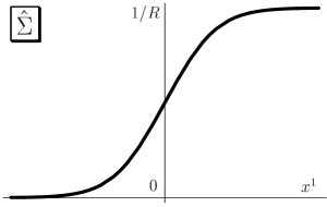
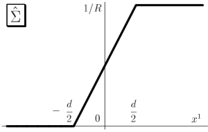
(a)	(b)

Fig. 3: Profiles of $\hat{\Sigma}(x^{1})$ before and after taking the limit $g^{2}c,1/R\rightarrow\infty$ with $d\equiv 2/g^{2}cR$ finite.

We have previously shown both from field theory [30] and string theory (the $s$-rule) [28] that these domain walls cannot pass through nor be compressed with each other. Therefore these objects can be regarded as 1-codimension rigid bodies with length $d$. Using this fact, we can map the multi-vortex system to the gas of hard rods, namely 1-dimensional gas of the rigid bodies.

Using the above limit, where the domain walls are regarded as the hard rods in 1-dimension, let us now consider the vortices on a torus $T^{2}$ with periods $2\pi R$ and $2\pi R^{\prime}$ and dual domain wall configuration space. Fig. 4-(a) shows the profile of $\hat{\Sigma}(x^{1})$ and Fig. 4-(b) shows the corresponding system of hard rods.

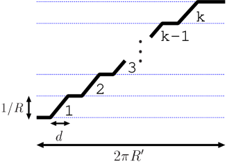
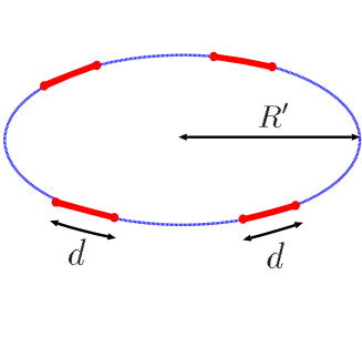
(a) Profile of $\hat{\Sigma}(x^{1})$	(b) 1-d gas of hard rods on $S^{1}$

Fig. 4: Profile of $\hat{\Sigma}(x^{1})$ for vortices and corresponding 1-d gas of hard rods.

For the gas of identical hard rods with mass $m$ on $S^{1}$ with period $L$, the classical partition function can be easily calculated as

$$Z_{\rm rods}=\frac{1}{k!}\left(\frac{mT}{2\pi}\right)^{k}L\left(L-kd\right)^{k-1}.$$ (3.7)

In this case, the period is $L=2\pi R^{\prime}$ and each rod has mass $m=2\pi c$ which corresponds to the mass of the vortex. There are additional phase degrees of freedom which correspond to the positions of vortices in $x^{2}$-direction. In the limit $g^{2}c,1/R\rightarrow\infty$ with $d=\frac{2}{g^{2}cR}$ finite, these phase degrees of freedom become independent and have the period $2\pi R$. In other words, the T-duality maps the FI-parameter $c$ to $2\pi Rc$. So we should replace $c$ by $2\pi Rc$ in the vortex picture. (Note that the combination $d=\frac{2}{g^{2}cR}$ is invariant under the T-duality.) Therefore the partition function of $k$-vortex system on a torus $T^{2}$ is given by

$$Z^{N_{\rm C}=N_{\rm F}=1}_{k,T^{2}}=\frac{1}{k!}\left(cT\right)^{k}2\pi R^{\prime}\left(2\pi R^{\prime}-kd\right)^{k-1}\left(2\pi R\right)^{k}=\frac{1}{k!}\left(cT\right)^{k}A\left(A-\frac{4\pi k}{g^{2}c}\right)^{k-1},$$ (3.8)

where $A=(2\pi)^{2}RR^{\prime}$ is the area of $T^{2}$. This result coincides with the exact partition function which has already been known [3, 4, 5]. The inequality (2.5) with $N_{\rm C}=1$ implies that the number of vortices $k$ must be less than $\frac{g^{2}c}{4\pi}A$. In the Bradlow limit $k=\frac{g^{2}c}{4\pi}A$, the partition function Eq. (3.8) vanishes. In our interpretation of vortices as 1-dimensional rods, this maximum number can be understood from the fact that sum of the length of rods can not exceed the compact period of $S^{1}$, namely $\frac{2k}{g^{2}cR}=kd\leq 2\pi R^{\prime}$ from the first equation of (3.2).

We can derive the van der Waals equation of state for the vortex gas in the thermodynamic limit $A\to\infty$, $k\to\infty$ with keeping $k/A$ fixed (see eg. §7.15 in [5]),

$$P\left(A-\frac{4\pi k}{g^{2}c}\right)=kT.$$ (3.9)

Here $P$ is the pressure of the vortex gas and the Boltzman constant is unity $(k_{B}=1)$ in our notation. From this we find the pressure of the vortex gas diverges at the maximal number of vortices determined by the area and couplings. Compared with the general van der Waals equation of state $\left(P+ak^{2}/A^{2}\right)\left(A-kb\right)=kT$ we have $a=0$ and $b=4\pi/(g^{2}c)$. The former can be understood as the BPS property that there exists no potential energy between BPS vortices. The latter implies the size (exclusion area) of the ANO vortex is $4\pi/(g^{2}c)$.

4 Local/Semi-local Non-Abelian Vortices

So far we have seen that the partition function for multi-vortex system can be calculated by using a system of hard rods in the case of the Abelian-Higgs model ($N_{\rm C}=N_{\rm F}=1$). We next extend this method to the more general cases of non-Abelian and Abelian gauge theories: local non-Abelian vortices ($N_{\rm C}=N_{\rm F}>1$) and semi-local (non-Abelian) vortices ($N_{\rm F}>N_{\rm C}$). These cases were not known previously, which proves the power of our method. To this end, we treat vortices in a model with a twisted boundary condition

$$H(x^{1},x^{2}+2\pi R)=H(x^{1},x^{2})e^{2\pi iRM},$$ (4.1)

where $M={\rm diag}(\alpha_{1}/R,\cdots,\alpha_{N_{\rm F}}/R),~{}\alpha_{1}<\cdots<\alpha_{N_{\rm F}}<1+\alpha_{1}$. We can reproduce the partition function with ordinary boundary condition by taking the limit $\alpha_{A}\rightarrow 0$ after calculating the partition function with the twisted boundary condition. In this case, $k$-vortex configuration corresponds to $kN_{\rm F}$ domain walls represented as kinks of the eigenvalues of $\hat{\Sigma}(x^{1})$ as shown in Fig. 5. By taking the limit (3.1), we can identify each domain wall with a 1-dimensional rod as before. In this limit, all kinks of $\hat{\Sigma}(x^{1})$ which correspond to domain walls have the same slope, which is $1/dR=g^{2}c/2$.

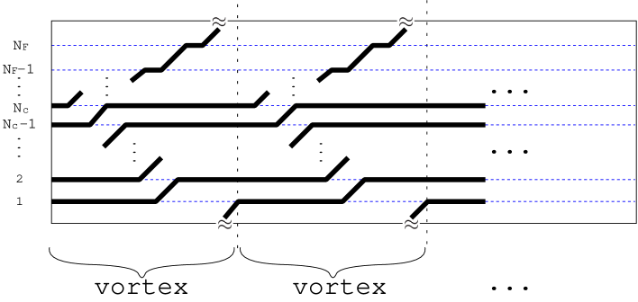
Fig. 5: Eigenvalues of $\hat{\Sigma}(x^{1})$ as the dualized configuration of $k$ vortices. Kinks represent $kN_{\rm F}$ domain walls.

In this case there are $N_{\rm F}$ types of rods whose masses are given by

$$m_{A} = 2\pi c(\alpha_{A+1}-\alpha_{A}),\hskip 14.22636ptA=1,\cdots,N_{\rm F}-1,$$

$$m_{N_{\rm F}} = 2\pi c(1+\alpha_{1}-\alpha_{N_{\rm F}}).$$ (4.2)

and the period of phases are given by

$$l_{A} = 2\pi R/(\alpha_{A+1}-\alpha_{A}),\hskip 14.22636ptA=1,\cdots,N_{\rm F}-1,$$

$$l_{N_{\rm F}} = 2\pi R/(1+\alpha_{1}-\alpha_{N_{\rm F}}).$$ (4.3)

Then we can calculate the partition function for the multi-vortex system in terms of the 1-dimensional hard rods. Note that we have to take into account the fact that there are $k$ indistiguishable sets of rods corresponding to $k$ indistinguishable vortices. Therefore the partition function should be divided by $k$ after integrating over the configuration space of distinguishable rods. Then the partition function for multi-vortex system takes the form of

$$Z^{N_{\rm C},N_{\rm F}}_{k,T^{2}} = \left(\frac{T}{2\pi}\right)^{kN_{\rm F}}\left(\prod_{A=1}^{N_{\rm F}}m_{A}l_{A}\right)^{k}\frac{1}{k}\int_{X}dx_{1}\cdots dx_{kN_{\rm F}}$$ (4.4)

$$= \left(\frac{T}{2\pi}\right)^{kN_{\rm F}}(2\pi c)^{kN_{\rm F}}(2\pi R)^{kN_{\rm F}}\frac{1}{k}\int_{X^{\prime}}dy_{1}\cdots dy_{kN_{\rm F}}.$$

Here the integration with respect to positions $\{x_{n}\}$ is taken over the configuration space of the rods, which is denoted as $X$. In the last line, we have redefined the coordinates as $y_{n}=x_{n}-\alpha_{A}d$ if the $n$-th rod sits between the $A$-th flavor and the ($A+1$)-th flavor, and the corresponding domain of integration is denoted as $X^{\prime}$. The redefinition of the positions corresponds to consider a slant torus (Fig. 6) where domain wall configurations are right-angled and perpendicular to the $x^{1}$-direction. Therefore we can associate the configurations of vortices with that of rods with length $d$ and particles with zero size pierced by the rods. Recalling the original profile of the kink solution, we can see there exist some overlapping rules of the rods; a part of rods which is divide by the particles can overlap with each other, but not be allowed for some of these. So we also introduce colored rods in order to clarify the exclusion rules of rods. (See Fig. 7.) Note that the above formula in the last line is completely independent of the parameters $\{\alpha_{A}\}$. Therefore, our result with the twisted boundary condition (4.1) (non vanishing $\alpha_{A}$) is applicable to the ordinary case with non-twisted boundary condition ($\alpha_{A}=0$).

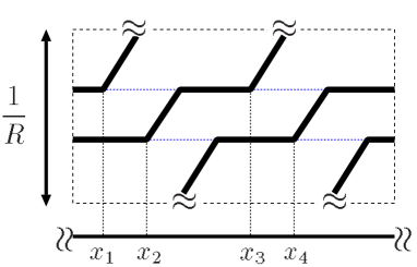
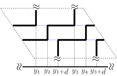
(a) Configuration for $N_{\rm C}=N_{\rm F}=2,k=2$	(b) Slant torus configuration

Fig. 6: The profile of eigenvalues of $\hat{\Sigma}(x^{1})$ and slant configuration for $N_{\rm C}=N_{\rm F}=2,k=2$.

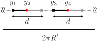
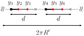
(a) $N_{\rm C}=N_{\rm F}=2,k=2$	(b) $N_{\rm C}=N_{\rm F}=3,k=2$

Fig. 7: (a) Configuration of rods (${}_{\blacksquare}\!\!\!-\!\!\!-\!_{\blacksquare}$) and particles ($\bullet$) pierced by the rods for $N_{\rm C}=N_{\rm F}=2,k=2$ corresponding Fig. 6. (b) Those for $N_{\rm C}=N_{\rm F}=3,k=2$. Each rod is divided by particles into the $N_{\rm C}$ parts with different colors. Each part of rods can overlap with parts of the other rods with different colors but not with parts with the same color.

The partition function Eq. (4.4) can be interpreted as the asymptotic form of partition function of vortex gas on the rectangular torus in the limit Eq. (3.1). Let us assume that the partition function is independent of details of the torus and depends only on the area of torus $A$. This is the case for the partition function in the model with $N_{\rm C}=N_{\rm F}=1$. Then we can calculate the partition function for vortex gas on a surface which is topologically a rectungular torus with area $A$. In addition, we can show that Eq. (4.4) gives the exact form of partition function as follows: The limit Eq. (3.1) can be rewritten as

$$R=\frac{R_{0}}{\mu},\hskip 14.22636ptc=\mu c_{0},\hskip 14.22636pt\mu\rightarrow\infty,\hskip 14.22636ptR_{0},c_{0},g:{\rm fixed}.$$ (4.5)

From the explicit expression of the metric of moduli space [15] and dimensional analysis, we can show that the partition function takes the form of

$$Z^{N_{\rm C},N_{\rm F}}_{k,T^{2}} = (cT)^{kN_{\rm F}}A^{kN_{\rm F}}f(g^{2}cA)$$ (4.6)

$$= (c_{0}T)^{kN_{\rm F}}{A_{0}}^{kN_{\rm F}}f(g^{2}c_{0}A_{0}),\hskip 28.45274ptA_{0}\equiv(2\pi)^{2}R_{0}R^{\prime}$$

where $f(g^{2}cA)$ is an unknown funtion of dimensionless parameter $g^{2}cA$. From this expression, we find that the partition function is independent of $\mu$. Therefore the limit $\mu\rightarrow\infty$ gives the exact partition function. In the discussion below, we assume that the partition function depends only on the area of torus $A$. We will check that the partition function Eq. (4.4) indeed gives the exact result for one vortex with $N_{\rm C}=N_{\rm F}=N$ and $N_{\rm F}>N_{\rm C}=1$.

We now perform the integration in (4.4) explicitly in some cases, all of which are new results.

1) Two ($\boldsymbol{k=2}$) local non-Abelian vortices with $\boldsymbol{N_{\rm C}=N_{\rm F}=2}$

Let us consider the domain of integration for $N_{\rm C}=N_{\rm F}=2$ and $k=2$ for example. The domain can be easily seen from Fig. 6 and Fig. 7-(a). In this case there are two rods with one particle inside each of them. These rods can overlap with each other contrary to the case of $N_{\rm C}=N_{\rm F}=1$. However the edges of the rods cannot overlap with the particles inside the other rods. Therefore the domain of integration is given by

$$X^{\prime}=\left\{(y_{1},y_{2},y_{3},y_{4})\left|\begin{array}[]{ccc}0<y_{1}<2\pi R^{\prime},&y_{1}<y_{2}<y_{1}+d,&y_{2}<y_{3},\hskip 14.22636pty_{1}+d<y_{4},\\ y_{3}<y_{4}<y_{3}+d,&y_{3}+d<y_{2}+2\pi R^{\prime},&y_{4}<y_{1}+2\pi R^{\prime},\end{array}\right.\right\}.$$ (4.9)

Performing the integral in Eq. (4.4) over the domain (4.9), we immediately obtain the partition function of the vortices (the volume of the domain wall (rods with particles) configuration space)

$$Z^{N_{\rm C}=2,N_{\rm F}=2}_{k=2,T^{2}}=\left\{\begin{array}[]{llc}\dfrac{1}{2}(cT)^{4}\left(\dfrac{4\pi}{g^{2}c}\right)^{2}A\left(A-\dfrac{2}{3}\dfrac{8\pi}{g^{2}c}\right)&\qquad\mbox{ for }&\dfrac{8\pi}{g^{2}c}\leq A\\ \dfrac{1}{6}(cT)^{4}\left(A-\dfrac{4\pi}{g^{2}c}\right)^{2}A\left(\dfrac{16\pi}{g^{2}c}-A\right)&\qquad\mbox{ for }&\dfrac{4\pi}{g^{2}c}\leq A\leq\dfrac{8\pi}{g^{2}c}\end{array}\right..$$ (4.12)

Note that there exists a lower bound for the area $A\geq 4\pi/(g^{2}c)$ which corresponds to the Bradlow limit (2.5). This is a new result which was not derived previously. Let us explain the physical meaning of each factor restricting us to the first case. Remembering that each vortex carries an internal orientation of $\mathbb{C}P^{1}$, we can understand that the factor $(4\pi/(g^{2}c))^{2}$ corresponds to the internal orientations (see Eq. (4.13) with $N=2$ below) while the factor $A$ does to the center of mass. Then the remaining factor $A-\frac{2}{3}\frac{8\pi}{g^{2}c}$ can be thought of as effective area of relative motion moduli of two non-Abelian vortices. Comparing this result to that of two Abelian vortices in Eq. (3.8) with $k=2$, the extra factor $2/3$ appears here, which implies that the effective area of non-Abelian vortices is smaller than that of Abelian vortices. Interestingly, the factor 2/3 in the exclusion area is different from the factor 1/2 in the Bradlow area $B_{2}=\frac{1}{2}\frac{4\pi}{g^{2}c}$, contrary to the Abelian case Eq. (3.9) in which the both factors coincide. We will see this in more detail around (4.16), below.

2) $\boldsymbol{k}$ Local non-Abelian vortices with $\boldsymbol{N_{\rm C}=N_{\rm F}=N}$

Let us next consider the single ($k=1$) non-Abelian vortex. In this case the moduli space is $T^{2}\times\mathbb{C}P^{N-1}$. The corresponding configuration has a rod and $N-1$ particles trapped inside a rod, see Fig. 8-(ii)-(a).

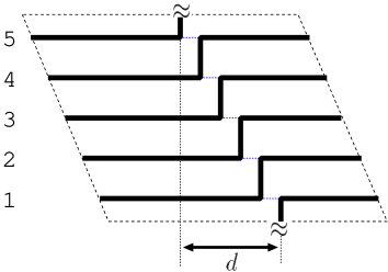
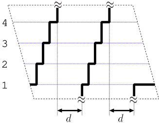
(a) $N_{\rm C}=N_{\rm F}=5,~{}k=1$	(b) $N_{\rm C}=1,~{}N_{\rm F}=4,~{}k=2$
(i) Configurations of eigenvalues of $\hat{\Sigma}(x^{1})$ on slant torus.

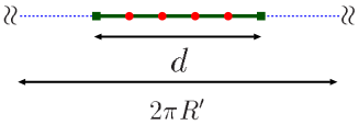
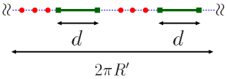
(a) $N_{\rm C}=N_{\rm F}=5,~{}k=1$	(b) $N_{\rm C}=1,~{}N_{\rm F}=4,~{}k=2$
(ii) Configurations of rods and particles.

Fig. 8: Examples of stant configurations on eigenvalues of $\hat{\Sigma}(x^{1})$ and corresponding rods and paricles. (i)-(a) There are 4 small kinks trapped in the region with length $d$. (i)-(b) There are 3 small kinks trapped in each interval between two regions with length $d$. (ii)-(a) There are 4 particles trapped inside a rod. (ii)-(b) There are 3 particles trapped in each interval between 2 hard rods.

The partition function (4.4) is defined only in the region $A\geq 4\pi/(g^{2}c)$ since the number of eigenvalues of $\hat{\Sigma}(x_{1})$ is $N_{\rm C}$ and the period $2\pi R^{\prime}$ should be larger than the length $d$ of a rod: namely this bound is the second inequality in Eq. (3.2),

$$Z^{N_{\rm C}=N_{\rm F}=N}_{k=1,T^{2}} = \left(\frac{T}{2\pi}\right)^{N}(2\pi c)^{N}(2\pi R)^{N}2\pi R^{\prime}\frac{1}{(N-1)!}d^{N-1}$$ (4.13)

$$= \frac{1}{(N-1)!}\left(cT\right)^{N}A\left(\frac{4\pi}{g^{2}c}\right)^{N-1}.$$

In this simple case, we can confirm that our result agrees with an explicit integration over the exact metric on the non-Abelian vortex moduli space. Although the solution is not known, the metric with the Kähler class can be calculated [12, 31], to give

$$ds^{2}=2\pi c\,dzd\bar{z}+\frac{8\pi}{g^{2}}\frac{\delta_{i\bar{j}}(1+|b^{k}|^{2})-\bar{b}^{i}b^{j}}{\left(1+|b^{k}|^{2}\right)^{2}}db^{i}d\bar{b}^{j},$$ (4.14)

where $b^{i}$ are the inhomogeneous coordinates of orientational moduli $\mathbb{C}P^{N-1}$. Using this metric, we can confirm that Eq. (4.13) agrees with the correct partition function.

For general number $k$ of the non-Abelian vortices with $N_{\rm C}=N_{\rm F}=N$, we can calculate the partition function (4.4) up to the next leading term in the expansion in terms of $1/A$

$$Z^{N_{\rm C}=N_{\rm F}=N}_{k,T^{2}}=\left(cT\right)^{kN}\frac{1}{k!}\left[\frac{A}{(N-1)!}\left(\frac{4\pi}{g^{2}c}\right)^{N-1}\right]^{k}\left[1-D_{N}(k-1)\frac{k}{A}+\mathcal{O}\left(\left(\frac{4\pi}{g^{2}cA}\right)^{2}\right)\right].$$ (4.15)

We can show that the coefficient $D_{N}$ in Eq. (4.15) takes the form (the definition of $D_{N}$ is given in Appendix)

$$\frac{D_{N}}{4\pi/g^{2}c}=\frac{(2N-2)!!}{(2N-1)!!}=1,\;{2\over 3},\;{8\over 15},\;{16\over 35},\;{128\over 315},\cdots\;\quad(N=1,2,3,4,5,\cdots).$$ (4.16)

The first (leading) term in the partition function (4.15) represents the situation that all vortices are separated, while the second (next leading) term implies that a pair of adjacent vortices is overlaped. From the partition function (4.15), we can obtain the equation of state for dilute vortex gas in the thermodynamic limit $A\rightarrow\infty,k\rightarrow\infty$ with fixing $k/A$ to enough small value as

$$PA\left(1-D_{N}\frac{k}{A}+{\cal O}\left(\frac{k^{2}}{A^{2}}\right)\right)=kT.$$ (4.17)

From this we see that the second virial coefficient $D_{N}$ represents the effective area of the non-Abelian vortices in dilute gas. We find that the third term $\mathcal{O}(k^{2}/A^{2})$ does not vanish. This implies that the equation of state deviates from van der Waals one, contrary to the Abelian case Eq. (3.8).

We find that $D_{N}<D_{1}=\frac{4\pi}{g^{2}c}$ and $D_{N}$ begaves as

$$D_{N}\sim\frac{1}{2}\sqrt{\frac{\pi}{N}}\frac{4\pi}{g^{2}c}$$ (4.18)

for large $N$. We see that the non-Abelian vortices can be closer to each other than the Abelian vortices even though the area of individual vortex is $\frac{4\pi}{g^{2}c}$ for both non-Abelian and Abelian vortices. Therefore we conclude that non-Abelian vortices are “softer” than Abelian vortices.

Clearly the inequality $B_{N}<D_{N}$ holds with $B_{N}=\frac{1}{N}\frac{4\pi}{g^{2}c}$ being the Bradlow area in (2.5). This inequality implies that the effective area $D_{N}$ of a vortex in dilute vortex gas is larger than the Bradlow area $B_{N}$, which is the effective area in highly pressured gas. An intuitive understanding of this inequality is as follows. It is known that the internal orientations of two non-Abelian vortices are almost always aligned when the two vortices are approaching each other [20] (as long as their speed is sufficiently slow). In other words, nearby non-Abelian local vortices behave as if they are Abelian local vortices.

3) $\boldsymbol{k}$ semi-local vortices with $\boldsymbol{N_{\rm C}=1}$ and general $\boldsymbol{N_{\rm F}}$

Finally we show that our method can be extended to the case of semi-local vortices with $N_{\rm F}>N_{\rm C}$. Here we concentrate on the $N_{\rm C}=1$ case which indicates essential features of semi-local vortices. The corresponding configuration has $N_{\rm F}-1$ particles trapped in each interval between $k$ hard rods, see Fig. 8-(b). In this case, Eq. (4.4) reduces to

$$Z^{N_{\rm C}=1,N_{\rm F}}_{k,T^{2}} = \left(\frac{T}{2\pi}\right)^{kN_{\rm F}}(2\pi c)^{kN_{\rm F}}(2\pi R)^{kN_{\rm F}}\frac{1}{k}\frac{1}{(kN_{\rm F}-1)!}2\pi R^{\prime}\left(2\pi R^{\prime}-dk\right)^{kN_{\rm F}-1}$$ (4.19)

$$= \left(cT\right)^{kN_{\rm F}}\frac{1}{k}\frac{1}{(kN_{\rm F}-1)!}A\left(A-\frac{4\pi k}{g^{2}c}\right)^{kN_{\rm F}-1},$$

where $1/k$ factor is needed since $k$ vortices cannot be distinguished. Substituting $N_{\rm F}=1$ into this result, the partition function of $k$ ANO vortices in Eq. (3.8) is correctly recovered. From this partition function, we can obtain the equation of state for the vortex gas in the thermodynamic limit $A\rightarrow\infty,k\rightarrow\infty$ with $k/A$ finite as

$$P\left(A-\frac{4\pi k}{g^{2}c}\right)=kN_{\rm F}T,$$ (4.20)

where $P$ is the pressure. The factor $N_{\rm F}$ in the right hand side of Eq. (4.20) appears due to the fact that the vortices have additional internal degrees of freedom in the case of $N_{\rm F}>1$.

In this case, no field theoretical result has been known yet. Especially we can show that the moduli space of $k=1$ semilocal vortex (see Fig. 8-(b)) is $T^{2}\times{\mathbb{C}}P^{N_{\rm F}-1}$ by extending the moduli matrix formalism [15] to $T^{2}$. Second, as was done in [31], we can compute the moduli space metric by using the integration formula of the Kähler potential in [17], to give

$$ds^{2}=2\pi c\,dzd\bar{z}+2c\left(A-\frac{4\pi}{g^{2}c}\right)\frac{\delta_{i\bar{j}}(1+|b^{k}|^{2})-\bar{b}^{i}b^{j}}{\left(1+|b^{k}|^{2}\right)^{2}}db^{i}d\bar{b}^{j}.$$ (4.21)

Here $b^{i}$ in the second term are the inhomogeneous coordinates of $\mathbb{C}P^{N_{\rm F}-1}$ and represent moduli not localized around vortices. These moduli become non-normalizable on the plane $\mathbb{C}$ ($A\rightarrow\infty$). However they contribute to the Kähler potential since we are considering the vortices on the compact manifold $T^{2}$ with the finite area $A$. From this metric we can confirm at least for $k=1$ case that Eq. (4.19) gives the correct partition function.

5 Comments and Discussions

We here comment on an important fact that there is a duality on the partition function (4.4), without performing the difficult integration. That is, the partition function for $k\leq N_{\rm C}$ is invariant under exchange

$$\left(N_{\rm C},\,g^{2}\right)\leftrightarrow\left(\widetilde{N}_{\rm C},\,\tilde{g}^{2}\right),$$ (5.1)

$${\rm with~{}} \widetilde{N}_{\rm C}\equiv k+N_{\rm F}-N_{\rm C},\quad{4\pi\over\tilde{g}^{2}c}\equiv A-{4\pi\over g^{2}c}.$$

One can confirm that this duality exists between the partition function (4.13) and the one of the $k=1$ case of (4.19). Also, the example of $N_{\rm C}=N_{\rm F}=2,k=2$ is self-dual. In fact, in the partition function (4.12), the latter case ($A/2\leq 4\pi/(g^{2}c)$) can be obtained by exchanging $4\pi/(g^{2}c)$ by $A-4\pi/(g^{2}c)$ in the former case ($A/2\geq 4\pi/(g^{2}c)$). These observations are very analogous to the duality relation between the non-commutative instantons and monopoles [32, 33]. From string theoretical point of view, there appears a slant torus due to the effect of the magnetic gauge field or equivalently the $B$-field. The $B$-field is a source of the non-commutativity and associated with the FI parameters in the effective theory on the instantons. In our case, the gauge coupling plays a role of the non-commutative parameter and should relate to the modulus of the slant torus. Better explanation on the above duality may be found in terms of the duality between the non-commutative vortex and domain wall in the string theoretical picture.

Finally we would like to discuss vortices on a sphere $S^{2}$. In this case we cannot use the above T-dual argument naively since the sphere consists of non-trivial $U(1)$ fibration. However we here assume that the vortices on the sphere is equivalent to the vortices on the cylinder with finite length in the computation of the volume of the moduli space; The cylinder is topologically isomorphic to the sphere with two puncture points. When at least one vortex sits on a puncture point (the notrh or south pole) of the sphere, the dimension of the corresponding subspace is less than the dimension of the full moduli space. Therefore this subspace does not contribute to the volume of the moduli space. In contrast to the torus case, we do not need to identify the both sides in the $x^{1}$-direction. Thus it is now sufficient to consider the gas of the hard rods in a finite segment with length $2\pi R^{\prime}$. By using the system of the hard rods, we obtain the partition function of vortices in the Abelian-Higgs model on $S^{2}$ as

$$Z^{N_{\rm C}=N_{\rm F}=1}_{k,S^{2}}=\frac{1}{k!}\left(cT\right)^{k}\left(2\pi R^{\prime}-kd\right)^{k}\left(2\pi R\right)^{k}=\frac{1}{k!}\left(cT\right)^{k}\left(A-\frac{4\pi k}{g^{2}c}\right)^{k}.$$ (5.2)

This completely agrees with the results in [2, 4, 5]. This case also should be extendable to the non-Abelian and/or semi-local vortices.

In conclusion, we have proposed a novel and simple method to compute the partition function of vortices at finte temperature. Our result agrees with previously known cases (3.8) and (5.2) of the local Abelian (ANO) vortices in the Abelian-Higgs model on $T^{2}$ and $S^{2}$, respectively. Our method provides new results in more general cases of non-Abelian local vortices, (4.12) and (4.15), and Abelian semi-local vortices, (4.19). In the two cases of $k=1$, $N_{\rm C}=N_{\rm F}=N$ and $k=1$, $N_{\rm C}=1$ with general $N_{\rm F}$, we have confirmed that our results agree with explicit integrations over the exact moduli metrics (4.14) and (4.21), respectively. We have found that non-Abelian vortices are reduced under T-duality to soft rods with particles inside them while the Abelian vortices are to hard rods.

Our results will be applied to the thermal vortex gas in the early Universe or in superconductor. Extension to non-(or near-)critical coupling will be important to discuss more realistic application. In particular the phase transition of vortex gas in the Abelian-Higgs model was discussed previously [34, 35]. Presence or absence of phase transitions in the non-Abelian and/or semi-local vortices is very interesting to explore.

Appendix A Virial Expansion

In this appendix we give the defenition of $D_{N}$ which appears as a coefficient of the next leading term in the partition function (4.15). We consider $k$ non-Abelian local vortices with $N_{\rm C}=N_{\rm F}=N$ on a torus $T^{2}$. As we have mentioned, the system can be well described from the picture of $k$ soft rods with length $d$, each of them piercing $N-1$ particles therein, on $S^{1}$ in circumference $L=2\pi R^{\prime}$, as shown in Fig. 5. We can carry out an integration with respect to only $k$ parameters corresponding to positions of the rods and we find that the volume of the configuration space can be rewritten as

$$V_{N,k}\equiv\frac{1}{k}\int d^{kN}y=\frac{\left(Ld^{N-1}\right)^{k}}{k!}\int_{\Sigma_{N,k}}d^{k(N-1)}z\left[\max\left(1-\frac{d}{L}\sum_{i=1}^{k}M_{N,i}\,\,,\,0\right)\right]^{k-1},$$ (A.1)

where the integration parameters $z=z_{r,i},(r=1,\cdots,N-1,i=1,\cdots,k)$ are dimensionless and correspond to $(N-1)$ relative positions of the particles inside each rod, and their integration region is defined by $\Sigma_{N,k}=\left\{\{z_{r,i}\}\big{|}0\leq z_{1,i}\leq z_{2,i}\leq\cdots\leq z_{N-1,i}\leq 1,1\leq i\leq k\right\}$. Here we have defined a dimensionless function, $M_{N,i}$, for each rod ($1\leq i\leq k$),

$$M_{N,i} = \max(z_{1,i},z_{2,i}-z_{1,i+1},\cdots,z_{N-1,i}-z_{N-2,i+1},1-z_{N-1,i+1}),$$ (A.2)

where we have defined $z_{r,k+1}=z_{r,1}$. All of them give the same contributions to the integration. Note that dimensionless parameter $d/L$ appears in the integrand. We find $kd\geq d\sum_{i}M_{N,i}$ in this case of local vortices. Thus small $kd/L$ guarantees that $L\geq d\sum_{i}M_{N,i}$ in any point of the integration region and that the integrand can be expanded with respect to $d/L$, since the max-function in Eq. (A.2) can be ignored. The $D_{N}$ appears as the coefficient of the next leading term in this expansion of $V_{N,k}$, namely in the virial expansion of soft rods in one dimension:

$$V_{N,k}=\frac{1}{k!}\left(\frac{Ld^{N-1}}{(N-1)!}\right)^{k}\left(1-\hat{D}_{N}\times k(k-1)\frac{d}{L}+{\cal O}\left(\frac{d^{2}}{L^{2}}\right)\right),$$ (A.3)

where we have defined $\hat{D}_{N}$ as an average value of $M_{N,1}$:

$$\hat{D}_{N} = \frac{1}{N}+\left((N-1)!\right)^{2}\int_{\begin{subarray}{c}\\ \\ 0\leq z_{1}\leq\cdots\leq z_{N-1}\leq 1\\ 0\leq z^{\prime}_{1}\leq\cdots\leq z^{\prime}_{N-1}\leq 1\end{subarray}}\!\!\!\!\!\!\!\!\!\!\!\!\!\!\!\!\!\!\!\!\!\!\!\!\!\!\!\!dz^{N-1}dz^{{}^{\prime}N-1}\ \max\left(z_{1}-z_{1}^{\prime},\cdots,z_{N-1}-z^{\prime}_{N-1},0\right),$$ (A.4)

where $\hat{D}_{N}$ relates with $D_{N}$ by $D_{N}=\hat{D}_{N}\frac{4\pi}{g^{2}c}=\hat{D}_{N}2\pi Rd$. We can easily carry out this integration in each region where a definite order of the integration parameters such as $z_{1}<z_{1}^{\prime}<z_{2}^{\prime}<z_{2}<\cdots$. It is convenient to divide the integration regions into several ones whose integral become identical. Therefore calculation for $D_{N}$ reduces to counting number of elements of the sets and we have succeeded this counting and obtained the result as (4.16).

References

- [1] N. A. Nekrasov, Adv. Theor. Math. Phys. 7 (2004) 831 [arXiv:hep-th/0206161]; [arXiv:hep-th/0306211].
- [2] N. S. Manton, Nucl. Phys. B 400 (1993) 624.
- [3] P. A. Shah and N. S. Manton, J. Math. Phys. 35 (1994) 1171 [arXiv:hep-th/9307165].
- [4] N. S. Manton and S. M. Nasir, Commun. Math. Phys. 199 (1999) 591 [arXiv:hep-th/9807017]; S. M. Nasir, Phys. Lett. B 419 (1998) 253 [arXiv:hep-th/9807020].
- [5] N. S. Manton and P. Sutcliffe, “Topological solitons,” Cambridge, UK: Univ. Pr. (2004)
- [6] N. M. Romao, J. Phys. A 38 (2005) 9127 [arXiv:hep-th/0503014].
- [7] A. A. Abrikosov, Sov. Phys. JETP 5 (1957) 1174 [Zh. Eksp. Teor. Fiz. 32 (1957) 1442]; H. B. Nielsen and P. Olesen, Nucl. Phys. B61 (1973) 45.
- [8] A. Hanany and D. Tong, JHEP 0307 (2003) 037 [arXiv:hep-th/0306150].
- [9] R. Auzzi, S. Bolognesi, J. Evslin, K. Konishi and A. Yung, Nucl. Phys. B 673 (2003) 187 [arXiv:hep-th/0307287].
- [10] D. Tong, Phys. Rev. D 69 (2004) 065003 [arXiv:hep-th/0307302].
- [11] R. Auzzi, S. Bolognesi, J. Evslin and K. Konishi, Nucl. Phys. B 686 (2004) 119 [arXiv:hep-th/0312233].
- [12] M. Shifman and A. Yung, Phys. Rev. D 70 (2004) 045004 [arXiv:hep-th/0403149];
- [13] A. Hanany and D. Tong, JHEP 0404 (2004) 066 [arXiv:hep-th/0403158].
- [14] M. Eto, Y. Isozumi, M. Nitta, K. Ohashi and N. Sakai, Phys. Rev. Lett. 96 (2006) 161601 [arXiv:hep-th/0511088].
- [15] M. Eto, Y. Isozumi, M. Nitta, K. Ohashi and N. Sakai, J. Phys. A 39 (2006) R315 [arXiv:hep-th/0602170].
- [16] M. Eto, K. Konishi, G. Marmorini, M. Nitta, K. Ohashi, W. Vinci and N. Yokoi, Phys. Rev. D 74, (2006) 065021 [arXiv:hep-th/0607070].
- [17] M. Eto, Y. Isozumi, M. Nitta, K. Ohashi and N. Sakai, Phys. Rev. D 73 (2006) 125008 [arXiv:hep-th/0602289].
- [18] K. Hashimoto and D. Tong, JCAP 0509 (2005) 004 [arXiv:hep-th/0506022]; R. Auzzi, M. Shifman and A. Yung, Phys. Rev. D 73 (2006) 105012 [arXiv:hep-th/0511150].
- [19] M. Eto, L. Ferretti, K. Konishi, G. Marmorini, M. Nitta, K. Ohashi, W. Vinci, N. Yokoi, arXiv:hep-th/0611313.
- [20] M. Eto, K. Hashimoto, G. Marmorini, M. Nitta, K. Ohashi and W. Vinci, Phys. Rev. Lett. 98 (2007) 091602 [arXiv:hep-th/0609214].
- [21] D. Tong, JHEP 0612 (2006) 051 [arXiv:hep-th/0610214]; A. Ritz, arXiv:hep-th/0612077.
- [22] L. G. Aldrovandi and F. A. Schaposnik, arXiv:hep-th/0702209.
- [23] D. Tong, Phys. Rev. D 66 (2002) 025013 [arXiv:hep-th/0202012].
- [24] M. Eto, T. Fujimori, Y. Isozumi, M. Nitta, K. Ohashi, K. Ohta and N. Sakai, Phys. Rev. D 73 (2006) 085008 [arXiv:hep-th/0601181].
- [25] N. S. Manton, Phys. Lett. B 110 (1982) 54.
- [26] S. B. Bradlow, Commun. Math. Phys. 135 (1990) 1.
- [27] N. D. Lambert and D. Tong, Nucl. Phys. B 569 (2000) 606 [arXiv:hep-th/9907098].
- [28] M. Eto, Y. Isozumi, M. Nitta, K. Ohashi, K. Ohta and N. Sakai, Phys. Rev. D 71 (2005) 125006 [arXiv:hep-th/0412024].
- [29] A. Hanany and E. Witten, Nucl. Phys. B 492 (1997) 152 [arXiv:hep-th/9611230].
- [30] Y. Isozumi, M. Nitta, K. Ohashi and N. Sakai, Phys. Rev. Lett. 93 (2004) 161601 [arXiv:hep-th/0404198]; Phys. Rev. D 71 (2005) 065018 [arXiv:hep-th/0405129]; Phys. Rev. D 70 (2004) 125014 [arXiv:hep-th/0405194]; M. Eto, Y. Isozumi, M. Nitta, K. Ohashi, K. Ohta, N. Sakai and Y. Tachikawa, Phys. Rev. D 71 (2005) 105009 [arXiv:hep-th/0503033].
- [31] M. Eto, Y. Isozumi, M. Nitta, K. Ohashi and N. Sakai, Phys. Rev. D 72 (2005) 025011 [arXiv:hep-th/0412048].
- [32] A. Hashimoto and K. Hashimoto, JHEP 9911, 005 (1999) [arXiv:hep-th/9909202]; K. Hashimoto, H. Hata and S. Moriyama, JHEP 9912, 021 (1999) [arXiv:hep-th/9910196]; K. Hashimoto and T. Hirayama, Nucl. Phys. B 587, 207 (2000) [arXiv:hep-th/0002090].
- [33] D. J. Gross and N. A. Nekrasov, JHEP 0007, 034 (2000) [arXiv:hep-th/0005204].
- [34] P. A. Shah, Nucl. Phys. B 438 (1995) 589 [arXiv:hep-th/9409145].
- [35] K. Kajantie, M. Laine, T. Neuhaus, A. Rajantie and K. Rummukainen, Nucl. Phys. B 559 (1999) 395 [arXiv:hep-lat/9906028].