String Theory, Space-Time Non-Commutativity and Structure Formation

Abstract

A natural consequence of string theory is a non-commutative structure of space-time on microscopic scales. The existence of a minimal length, and a modification of the effective field theory are two consequences of this space-time non-commutativity. I will first explore some consequences of the modifications of the effective field theory for structure formation in the context of an inflationary cosmology. Then, I will explore the possibility that the existence of a minimal length will lead to a structure formation scenario different from inflation. Specifically, I will discuss recent work on string gas cosmology.

1 Introduction and Summary

Non-commutativity of space-time on small scales appears to be one of the key consequences of string theory. Since cosmology provides what is probably the best way to test the consequences of new ultraviolet physics, I will in this talk explore some possible cosmological consequences of stringy space-time non-commutativity and of other key features of string theory.

If our universe underwent a period of cosmological inflation, then, since the physical wavelengths of scales we observe at the present time in observational cosmology started out smaller than the Planck length at the beginning of the period of inflation, it should be expected that the cosmological perturbations contain information about the ultraviolet completion of physics [1]. It has, in fact, been shown [2] that the results of the standard theory of cosmological perturbations (see e.g. [3] for an in-depth review, and [4] for a pedagogical overview) are not robust against modifications in the laws of physics on Planck scales. In Section 3 (following a preliminary section containing a brief summary of the essentials of the theory of cosmological perturbations), I will summarize work of [5] and [6] exploring the consequences of space-time non-commutativity on the spectrum of cosmological fluctuations. The main result is that, in the context of power-law accelerated expansion, the index of the spectrum changes: a spectrum which is slightly red according to the usual calculations becomes slightly blue on sufficiently large scales if space-time non-commutativity is taken into account.

Conventional scalar field-driven inflationary models, however, suffer from several conceptual problems (see e.g. [7, 8] for recent discussions). This motivates the search for cosmological backgrounds which do not require an inflationary period in order to explain the observational data. In Section 4 of this article, I will discuss a cosmological background [9] (“string gas cosmology”) which emerges if we make use of key stringy degrees of freedom and key symmetries of string theory.

In Section 5 I will summarize recent work [10, 11, 12] showing that, under certain conditions on the cosmological background, thermal fluctuations of a string gas in the very early universe can generate a scale-invariant spectrum of cosmological perturbations, hence providing an alternative to inflation for producing such a phenomenologically successful spectrum.

2 Brief Summary of the Theory of Cosmological Perturbations

If we neglect vector perturbations, gravitational waves, and anisotropic stress terms, the cosmological metric including fluctuations can be written in the form

$$ds^{2}\,=\,a^{2}\bigl{[}(1+2\phi)d\eta^{2}-(1-2\phi)dx^{2}\bigr{]}\,,$$ (1)

where $\eta$ is conformal time related to the physical time variable $t$ via $dt=a(\eta)d\eta$, $a(\eta)$ being the scale factor of the homogeneous and isotropic background cosmology, and the comoving spatial coordinates are denoted by $x$. The relativistic potential $\phi$ encodes the information about the scalar metric fluctuations and depends on space and time. To simplify the notation, we have taken the spatial background metric to be flat.

As matter we consider a scalar field $\varphi(x,\eta)$ which can be decomposed into a background component $\varphi_{0}(\eta)$ and a fluctuation $\delta\varphi(x,\eta)$. The action for the matter fluctuation in Fourier space is given by

$$S\,=\,\int d\eta d^{3}k{1\over 2}a^{2}(\eta)\bigl{(}\varphi^{\prime}_{-k}\varphi^{\prime}_{k}-k^{2}\varphi_{-k}\varphi_{k}\bigr{)}\,,$$ (2)

a prime denoting the derivative with respect to conformal time. The fields $\phi$ and $\delta\varphi$ are related via the Einstein constraint equations. The equations of motion for the fluctuations can be obtained by inserting the metric and matter field decompositions into the full action and expanding to quadratic order. The resulting action must reduce to that of a free scalar field $v$ with time-dependent mass. The two nontrivial tasks of the lengthy [3] computation of the quadratic piece $S^{(2)}$ of the action is to find out what combination of $\varphi$ and $\phi$ yields the variable $v$ in terms of which the action has canonical kinetic term, and what the form of the time-dependent mass is. The result is

$$S^{(2)}\,=\,{1\over 2}\int d^{4}x\bigl{[}v^{\prime 2}-v_{,i}v_{,i}+{{z^{\prime\prime}}\over z}v^{2}\bigr{]}\,,$$ (3)

where the canonical variable $v$ (the “Sasaki-Mukhanov variable” introduced in [13, 14, 15]) is given by

$$v\,=\,a\bigl{[}\delta\varphi+{{\varphi_{0}^{{}^{\prime}}}\over{\cal H}}\phi\bigr{]}\,$$ (4)

and

$$z\,=\,{{a\varphi_{0}^{{}^{\prime}}}\over{\cal H}}\,.$$ (5)

The variable $v$ is related to the curvature fluctuation ${\cal R}$ in comoving coordinates via $v=z{\cal R}$.

In momentum space, the equation of motion which follows from the action (3) is

$$v_{k}^{{}^{\prime\prime}}+k^{2}v_{k}-{{z^{{}^{\prime\prime}}}\over z}v_{k}\,=\,0\,,$$ (6)

where $v_{k}$ is the k’th Fourier mode of $v$. It follows that fluctuations oscillate on sub-Hubble scales (when $z^{{}^{\prime\prime}}/z$ is negligible), but freeze out and are squeezed $v\sim z$ on super-Hubble scales. If we choose vacuum initial conditions at an initial time $\eta_{i}$, then

$$v_{k}(\eta_{i})\,=\,{1\over{\sqrt{2k}}}$$ (7)

$$v_{k}^{{}^{\prime}}(\eta_{i})\,=\,{{\sqrt{k}}\over{\sqrt{2}}}\,.$$

The power spectrum of curvature perturbations, defined via

$$P_{k}\,={{k^{3}}\over{2\pi^{2}}}{{|v_{k}|^{2}}\over{z^{2}}}\,,$$ (8)

can then easily be calculated.

Note that gravitational waves and modes of a free scalar field on a fixed cosmological background obey a similar equation of motion, but with the function $z(\eta)$ replaced by the scale factor $a(\eta)$. If the equation of state of matter is constant in time, then $z(\eta)$ and $a(\eta)$ are proportional, but during a transition in the equation of state of matter, they are no longer proportional. In the standard example of such a transition, namely the transition during the phase of reheating in inflationary cosmology, $z(\eta)$ changes by a much larger factor than $a(\eta)$, thus leading to a larger squeezing for scalar cosmological fluctuations than for gravitational waves.

3 Space-Time Non-Commutativity and Inflationary Cosmology

In this section we will summarize the results of [5] in which the implications of space-time non-commutativity for the spectrum of cosmological fluctuations is explored. For consequences of space-space non-commutativity, the reader is referred to [16].

We start from the stringy space-time uncertainty relation [17]

$$\Delta t\Delta x_{p}\,\geq\,l_{s}^{2}\,,$$ (9)

where $t$ and $x_{p}$ are physical time and distance, respectively, and $l_{s}$ is the string length, and apply this relation to a cosmological space-time with scale factor $a(t)$ in terms of which the metric is given by

$$ds^{2}\,=\,dt^{2}-a(t)^{2}dx^{2}\,=\,a^{-2}(\tau)d\tau^{2}-a(\tau)^{2}dx^{2}\,,$$ (10)

where $\tau$ is a rescaled time. In terms of the new time variable $\tau$, the uncertainty relation (9) can be realized by imposing the deformed commutation relation

$$[\tau,x]_{*}\,=\,il_{s}^{2}$$ (11)

where the subscript $*$ implies that the products inside the commutator are given by the Moyal product

$$(f*g)(x,\tau)\,=\,e^{-{i\over 2}l_{s}^{2}(\partial_{x}\partial_{\tau^{\prime}}-\partial_{\tau}\partial_{y})}f(x,\tau)g(y,\tau^{\prime})$$ (12)

(evaluated at $y=x$ and $\tau^{\prime}=\tau$).

The uncertainty relation has two main effects on the cosmological perturbations. Firstly, it leads to an upper cutoff $k_{c}$ on the comoving momentum of fluctuation modes:

$$k_{c}(\tau)\,=\,{{a_{eff}(\tau)}\over{l_{s}}}\,,$$ (13)

where $a_{eff}$ is the scale factor smeared out over a time corresponding to the space-time uncertainty:

$$a^{2}_{eff}(\tau)\,=\,\bigl{(}{{\beta^{+}_{k}}\over{\beta^{-}_{k}}}\bigr{)}^{1/2}$$ (14)

with

$$\beta^{\pm}\,=\,{1\over 2}\bigl{[}a^{\pm 2}(\tau+kl_{s}^{2})+a^{\pm 2}(\tau-kl_{s}^{2})\bigr{]}\,.$$ (15)

Secondly, the uncertainty relation introduces a coupling between background geometry and fluctuations which is non-local in time, the non-locality being a consequence of the uncertainty in time. The theory of cosmological fluctuations in a non-commutative space-time can be obtained [5] from the theory in commutative space-time by taking the action (3) of cosmological perturbations and replacing the product operators by the Moyal product. For a real scalar field $\varphi$ on the background space-time, the modified action is [5]

$${\tilde{S}}\,=\,\int d\tau dx{1\over 2}\bigl{(}\partial_{\tau}\varphi^{\dagger}\star a^{2}\star\partial_{\tau}\varphi-\partial_{x}\varphi^{\dagger}\star a^{-2}\star\partial_{x}\varphi\bigr{)}\,.$$ (16)

which in momentum space becomes [5]

$${\tilde{S}}\,=\,\int_{k<k_{c}}d\eta d^{3}k{1\over 2}a_{k}^{2}(\tilde{\eta})\bigl{(}\varphi^{\prime}_{-k}\varphi^{\prime}_{k}-k^{2}\varphi_{-k}\varphi_{k}\bigr{)}\,,$$ (17)

where a prime indicates the derivative with respect to ${\tilde{\eta}}$,

$$a_{k}(\eta)\,=\,a(\eta)y_{k}(\eta)\,\,\,(y_{k}\,\equiv\,(\beta^{-}_{k}\beta^{+}_{k})^{1/4})\,,$$ (18)

and $d{\tilde{\eta}}=a_{eff}^{-2}d\tau$.

In the case of scalar metric fluctuations, the “smeared” function $a_{k}$ in (17) is replaced by a smeared function $z_{k}$ constructed in the same way from the “un-smeared” function $z$ as $a_{k}$ is from $a$. Thus, the net effect of non-commutativity on the evolution of cosmological fluctuations is that the function $z$ in the equation of motion (6) gets replaced by the smeared function $z_{k}$, yielding

$$v_{k}^{{}^{\prime\prime}}+k^{2}v_{k}-{{z_{k}^{{}^{\prime\prime}}}\over{z_{k}}}v_{k}\,=\,0\,.$$ (19)

We will be considering a background which yields power law inflation $a(t)\sim t^{n}$ with $n>1$, where the constant $n$ is related to the equation of state parameter $w=p/\rho$ ($p$ and $\rho$ being pressure and energy density, respectively) via

$$n\,=\,{2\over{3(1+w)}}\,.$$ (20)

Let us first consider UV modes, modes which are generated inside the Hubble radius. For these modes the value of $\Delta\tau$ is small in the sense that all smeared versions of the scale factor can be replaced by the scale factor itself. In this case, the analysis reduces to the usual analysis in the case of commutative space-time. The power spectrum of scalar metric fluctuations has a red tilt

$$P_{k}\,\sim\,k^{2/(1-n)}\,.$$ (21)

For IR modes, on the other hand, space-time non-commutativity leads to results which differ from the usual analysis. For these modes the space-time uncertainty relation is saturated at a time $\tau_{k}^{0}$ when the Hubble radius is smaller than the physical wavelength. At the time of saturation, the smearing of the scale factor is important. Effectively, the fluctuations evolve as if they had been generated not at the time $\tau_{k}^{0}$, but $\tau_{k}^{0}+kl_{s}^{2}$. Thus, there is less squeezing of the fluctuations then there would have been if the generation time had been $\tau_{k}^{0}$. This effect turns the red spectrum for UV modes into a blue spectrum for IR modes [5]

$$P_{k}\,\sim\,k^{3/(1+n)}\,.$$ (22)

For fixed value of $n$, the amount of the blue tilt for the $IR$ modes is identical to the amount of the red tilt for the $UV$ modes.

The change of the spectral tilt from red (on small angular scales) to blue (on large angular scales) could be used to explain the observed lack of power [18, 19] in the observed angular power spectrum of CMB fluctuations on the largest scales [6, 20].

Another interesting observation which follows from the work of [5] is the following: if we had treated the evolution of cosmological fluctuations with the un-modified perturbation equation (6) instead of with the modified equation (19), then - given vacuum initial conditions for the modes at the time when the physical wavelength is equal to a fixed cutoff scale - we would have obtained a scale-invariant spectrum for the IR modes for any expanding space-time, even if it is not accelerating. This point was stressed subsequently in [21].

It is important, however, to keep in mind that the physics which yields the minimal physical wavelength for the fluctuations will likely also effect the initial evolution, as it does in the non-commutative scenario discussed above. A further worry [22] concerning the model of [21] is that fluctuations on scales of observational interest to us today are generated when the Hubble radius is much smaller than the cutoff scale. It is hence possible that the cosmological background used is no longer consistent at the relevant early times.

4 Minimal Length and String Gas Cosmology

Since string theory is based on the quantization of extended objects, one expects string theory to give rise to the concept of a minimal observable length whose numerical value should be related to the string length $l_{s}$. For example, the location of the scattering point for the process of two initial strings scattering into two final strings is smeared out over the length scale of the string, and this is the reason that the cross-section for string scattering does not have the UV divergence which point particle scattering is affected with.

String gas cosmology [9] (see also [23] for early work and [24, 25] for reviews) is a toy model of string cosmology in which a minimal length scale clearly emerges. String gas cosmology is given by a background space-time (whose action will be discussed shortly) coupled to a gas of strings. Due to the extended nature of strings, there are degrees of freedom which do not exist in point particle theories. These degrees of freedom lead to a new symmetry specific to string theory, “T-duality”, a symmetry which implements the idea of a minimal length.

Taking all spatial directions to be toroidal (radius $R$), strings have three types of states: momentum modes which represent the center of mass motion of the string, oscillatory modes which represent the fluctuations of the strings, and winding modes counting the number of times a string wraps the torus. Both oscillatory and winding states are new features of string theory.

The energy of an oscillatory mode is independent of $R$, momentum mode energies are quantized in units of $1/R$, i.e. $E_{n}\,=\,n{1\over R}$ whereas the winding mode energies are quantized in units of $R$, i.e. $E_{m}\,=\,mR$ (both $n$ and $m$ are integers). Thus, we see that the energy spectrum of the string states admits a stringy symmetry called “T-duality symmetry”, namely a symmetry under the change $R\,\rightarrow\,1/R$ (in units of the string length $l_{s}$). Under this change, the energy spectrum of string states is not modified if $n$ and $m$ are interchanged. The string vertex operators are consistent with this symmetry. Postulating that T-duality extends to non-perturbative string theory leads [26] to the need of adding D-branes to the list of fundamental objects in string theory. With this addition, T-duality is expected to be a symmetry of non-perturbative string theory. Specifically, T-duality will take a spectrum of stable Type IIA branes and map it into a corresponding spectrum of stable Type IIB branes with identical masses [27].

It was argued in [9] that this symmetry leads to a minimal length. The argument goes as follows: Any physical detector will measure length in terms of the light degrees of freedom. At large values of $R$, these are the momentum modes, at small values of $R$ it is the winding modes. In terms of winding modes, the physics on a torus of radius $1/R$ is the same as the physics looks on a torus of radius $R$ in terms of momentum modes. Thus, the measured length $l_{phys}$ will satisfy $l_{phys}(1/R)\,=\,l_{phys}(R)$ and will therefore always be greater or equal to the string length.

A second important consequence of the stringy degrees of freedom for cosmology arises from the existence of a limiting temperature for a gas of strings in thermal equilibrium, the Hagedorn temperature $T_{H}$ [28]. Its existence follows from the fact that the number of string oscillatory modes increases exponentially as the string mode energy increases, there is a maximal temperature of a gas of strings in thermal equilibrium. Taking a box of strings and compressing it, the temperature will never exceed $T_{H}$. In fact, as the radius $R$ decreases below the string radius, the temperature will start to decrease, obeying the duality relation [9] $T(R)\,=\,T(1/R)$. Figure 1 provides a sketch of how the temperature $T$ changes as a function of $R$.

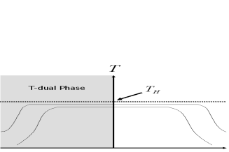
Figure 1: Sketch (based on the analysis of [9]) of the evolution of temperature $T$ as a function of the radius $R$ of space of a gas of strings in thermal equilibrium. The top curve is characterized by an entropy higher than the bottom curve, and leads to a longer region of Hagedorn behavior.

The conclusion from this analysis is that no temperature singularity is expected even if the mathematical background approaches the singular point $R\rightarrow 0$.

To obtain the dynamics of string gas cosmology, we need to specify an action for the background. This action must be consistent with the basic symmetries of string theory. Assuming, initially, that we are in the region of weak string coupling, the action can be taken to be that of dilaton gravity. The total action then is

$$S\,=\,{1\over{2\kappa^{2}}}\int d^{10}x\sqrt{-{\hat{g}}}e^{-2\phi}\bigl{[}{\hat{R}}+4\partial^{\mu}\phi\partial_{\mu}\phi\bigr{]}+S_{m}\,,$$ (23)

where ${\hat{g}}$ is the determinant of the metric, ${\hat{R}}$ is the Ricci scalar, $\phi$ is the dilaton, $S_{m}$ is the matter action (the hydrodynamical action of a gas of strings), and $\kappa$ is the reduced gravitational constant in ten dimensions. The metric appearing in the above action is the metric in the string frame.

In the case of a homogeneous and isotropic background given by

$$ds^{2}\,=\,dt^{2}-a(t)^{2}d{\bf x}^{2}\,,$$ (24)

the three resulting equations (the generalization of the two Friedmann equations plus the equation for the dilaton) in the string frame are [29] (see also [30])

$$-d{\dot{\lambda}}^{2}+{\dot{\varphi}}^{2}\, = \,e^{\varphi}E$$ (25)

$${\ddot{\lambda}}-{\dot{\varphi}}{\dot{\lambda}}\, = \,{1\over 2}e^{\varphi}P$$ (26)

$${\ddot{\varphi}}-d{\dot{\lambda}}^{2}\, = \,{1\over 2}e^{\varphi}E\,,$$ (27)

where $E$ and $P$ denote the total energy and pressure, respectively, $d$ is the number of spatial dimensions, and we have introduced the logarithm of the scale factor

$$\lambda(t)\,=\,{\rm log}(a(t))$$ (28)

and the rescaled dilaton

$$\varphi\,=\,2\phi-d\lambda\,.$$ (29)

From the second of these equations it follows immediately that a gas of strings containing both stable winding and momentum modes will lead to the stabilization of the radius of the torus: windings prevent expansion, momenta prevent the contraction. The right hand side of the equation can be interpreted as resulting from a confining potential for the scale factor. From this argument it immediately follows that a gas of strings containing both winding and momentum modes about the compact spatial dimensions leads to a stabilization of the radion modes (the radii of the extra dimensions) in the string frame [31]. Since the dilaton is not fixed in general, this does not correspond to a fixed radion in the Einstein frame. However, in the case of a gas of heterotic strings, it can be shown that enhanced symmetry states containing both momentum and winding modes lead to a stabilization of both volume [32] and shape [33] moduli (see also [34]). For a review of moduli stabilization in string gas cosmology, the reader is referred to [35].

5 String Gas Cosmology and Structure Formation

The equations of string gas cosmology discussed in the previous section lead to a new cosmological background. We begin in a Hagedorn phase during which the pressure vanishes (the positive pressure of the momentum modes canceling against the negative pressure of the winding modes) and thus the string frame scale factor is quasi-static. The decay of string winding modes into ordinary matter (string loops) will lead to a smooth transition to the radiation phase of standard cosmology. The dilaton comes to rest in the radiation phase. For reasons discussed in [36] (see also [37]) we need to assume that at early times in the Hagedorn phase ($t<t_{R}$) the dilaton is fixed. In the later stage of the Hagedorn phase which is described by the dilaton gravity action of the previous section the dilaton is running (decreasing with time).

This cosmological background yields the space-time diagram sketched in Figure 2. For times $t<t_{R}$, we are in the static Hagedorn phase and the Hubble radius is infinite. For $t>t_{R}$, the Einstein frame Hubble radius is expanding as in standard cosmology. The time $t_{R}$ is when the dilaton starts to decrease. At a slightly later time, the string winding modes decay, leading to the transition to the radiation phase of standard cosmology.

Given the assumptions specified above, string gas cosmology can lead to a causal mechanism of structure formation. We must compare the physical wavelength corresponding to a fixed comoving scale with the Einstein frame Hubble radius $H^{-1}(t)$. Recall that the Einstein frame Hubble radius separates scales on which fluctuations oscillate (wavelengths smaller than the Hubble radius) from wavelengths on which the fluctuations are frozen in and cannot be affected by micro-physics. Causal micro-physical processes can generate fluctuations only on sub-Hubble scales. The first key point is that for $t<t_{i}(k)$, the fluctuation mode $k$ is inside the Hubble radius, and thus a causal generation mechanism for fluctuations is possible. The second key point is that fluctuations evolve for a long time during the radiation phase outside the Hubble radius. This leads to the squeezing of fluctuations which is responsible for the acoustic oscillations in the angular power spectrum of CMB anisotropies (see e.g. [12] for a more detailed discussion of this point).

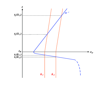
Figure 2: Space-time diagram (sketch) showing the evolution of fixed comoving scales in string gas cosmology. The vertical axis is time, the horizontal axis is physical distance. The solid curve represents the Einstein frame Hubble radius $H^{-1}$ which shrinks abruptly to a micro-physical scale at $t_{R}$ and then increases linearly in time for $t>t_{R}$. Fixed comoving scales (the dotted lines labeled by $k_{1}$ and $k_{2}$) which are currently probed in cosmological observations have wavelengths which are smaller than the Hubble radius before $t_{R}$. They exit the Hubble radius at times $t_{i}(k)$ just prior to $t_{R}$, and propagate with a wavelength larger than the Hubble radius until they reenter the Hubble radius at times $t_{f}(k)$.

Both in string gas cosmology and in the inflationary scenario, fluctuations emerge on sub-Hubble scales, thus allowing for a causal generation mechanism. However, the mechanisms are very different. In inflationary cosmology, the exponential expansion of space leaves behind a matter vacuum, and thus fluctuations originate as quantum vacuum perturbations. In contrast, in string gas cosmology space is static at early times, matter is dominated by a string gas, and it is thus string thermodynamical fluctuations which seed the observed structures.

The thermodynamics of a gas of strings was worked out some time ago. We take our three spatial dimensions to be compact (specifically $T^{3}$), thus admitting stable winding modes. Then, the string gas specific heat is positive, and in this context the string thermodynamics was studied in detail in [38].

Our procedure for string gas structure formation is the following. For a fixed comoving scale with wavenumber $k$ we compute the matter fluctuations while the scale in sub-Hubble (and therefore gravitational effects are sub-dominant). When the scale exits the Hubble radius at time $t_{i}(k)$ we use the gravitational constraint equations to determine the induced metric fluctuations, which are then propagated to late times using the usual equations of gravitational perturbation theory (see Section 2).

The metric including both scalar and tensor fluctuations is

$$ds^{2}=a^{2}(\eta)\left\{(1+2\Phi)d\eta^{2}-[(1-2\Phi)\delta_{ij}+h_{ij}]dx^{i}dx^{j}\right\}\,.$$ (30)

The spectra of cosmological perturbations $\Phi$ and gravitational waves $h$ are given by the energy-momentum fluctuations [12]

$$\langle|\Phi(k)|^{2}\rangle\,=\,16\pi^{2}G^{2}k^{-4}\langle\delta T^{0}{}_{0}(k)\delta T^{0}{}_{0}(k)\rangle\,,$$ (31)

brackets indicating expectation values, and

$$\langle|h(k)|^{2}\rangle\,=\,16\pi^{2}G^{2}k^{-4}\langle\delta T^{i}{}_{j}(k)\delta T^{i}{}_{j}(k)\rangle\,.$$ (32)

On the right hand side of (32), the average over the correlation functions with $i\neq j$ is implied, and $h$ indicates the amplitude of the gravitational wave $h_{ij}$.

The root mean square energy density fluctuations in a sphere of radius $R=k^{-1}$ are given by the specific heat capacity $C_{V}$ via

$$\langle\delta\rho^{2}\rangle\,=\,\frac{T^{2}}{R^{6}}C_{V}\,.$$ (33)

The result for the specific heat of a gas of closed strings on a torus of radius $R$ is [38]

$$C_{V}\,\approx\,2\frac{R^{2}/\ell_{s}^{3}}{T\left(1-T/T_{H}\right)}\,.$$ (34)

The power spectrum of scalar metric fluctuations is given by

$$P_{\Phi}(k)\, = \,8G^{2}k^{-1}<|\delta\rho(k)|^{2}>\,=\,8G^{2}k^{2}<(\delta M)^{2}>_{R}$$

$$= \,8G^{2}k^{-4}<(\delta\rho)^{2}>_{R}=\,8G^{2}{T\over{\ell_{s}^{3}}}{1\over{1-T/T_{H}}}\,,$$

where in the first step we have used (31) to replace the expectation value of $|\Phi(k)|^{2}$ in terms of the correlation function of the energy density, and in the second step we have made the transition to position space

The ‘holographic’ scaling $C_{V}(R)\sim R^{2}$ is responsible for the overall scale-invariance of the spectrum of cosmological perturbations. In the above equation, for a scale $k$ the temperature $T$ is to be evaluated at the time $t_{i}(k)$. Thus, the factor $(1-T/T_{H})$ in the denominator is responsible for giving the spectrum a slight red tilt.

As discovered in [39], the spectrum of gravitational waves is also nearly scale invariant. In the expression for the spectrum of gravitational waves the factor $(1-T/T_{H})$ appears in the numerator, thus leading to a slight blue tilt of the spectrum. This is a prediction with which the cosmological effects of string gas cosmology can be distinguished from those of inflationary cosmology, where quite generically a slight red tilt for gravitational waves results. The physical reason for the blue tilt is that large scales exit the Hubble radius earlier when the pressure and hence also the off-diagonal spatial components of $T_{\mu\nu}$ are closer to zero.

At the present time we are still lacking a good description of the background cosmology in the Hagedorn phase. A specific higher derivative gravity action in which a Hagedorn phase of string matter can be obtained with constant dilaton is given in [40].

References

- [1] R. H. Brandenberger, “Inflationary cosmology: Progress and problems,” publ. in proc. of IPM School On Cosmology 1999: Large Scale Structure Formation, arXiv:hep-ph/9910410.
-
[2]
R. H. Brandenberger and J. Martin, “The robustness of inflation to changes in super-Planck-scale physics,”
Mod. Phys. Lett. A 16, 999 (2001),
[arXiv:astro-ph/0005432];
J. Martin and R. H. Brandenberger, “The trans-Planckian problem of inflationary cosmology,” Phys. Rev. D 63, 123501 (2001), [arXiv:hep-th/0005209]. - [3] V. F. Mukhanov, H. A. Feldman and R. H. Brandenberger, “Theory Of Cosmological Perturbations. Part 1. Classical Perturbations. Part 2. Quantum Theory Of Perturbations. Part 3. Extensions,” Phys. Rept. 215, 203 (1992).
- [4] R. H. Brandenberger, “Lectures on the theory of cosmological perturbations,” Lect. Notes Phys. 646, 127 (2004) [arXiv:hep-th/0306071].
- [5] R. Brandenberger and P. M. Ho, “Noncommutative spacetime, stringy spacetime uncertainty principle, and density fluctuations,” Phys. Rev. D 66, 023517 (2002).
- [6] S. Tsujikawa, R. Maartens and R. Brandenberger, “Non-commutative inflation and the CMB,” Phys. Lett. B 574, 141 (2003) [arXiv:astro-ph/0308169].
- [7] R. H. Brandenberger, “Looking beyond inflationary cosmology,” arXiv:hep-th/0509076.
- [8] R. H. Brandenberger, “Conceptual Problems of Inflationary Cosmology and a New Approach to Cosmological Structure Formation,” arXiv:hep-th/0701111, to be publ. in the proceedings of Inflation + 25 (Springer, Berlin, 2007).
- [9] R. H. Brandenberger and C. Vafa, “Superstrings In The Early Universe,” Nucl. Phys. B 316, 391 (1989).
- [10] A. Nayeri, R. H. Brandenberger and C. Vafa, “Producing a scale-invariant spectrum of perturbations in a Hagedorn phase of string cosmology,” Phys. Rev. Lett. 97, 021302 (2006) [arXiv:hep-th/0511140].
- [11] A. Nayeri, “Inflation free, stringy generation of scale-invariant cosmological fluctuations in D = 3 + 1 dimensions,” arXiv:hep-th/0607073.
- [12] R. H. Brandenberger, A. Nayeri, S. P. Patil and C. Vafa, “String gas cosmology and structure formation,” arXiv:hep-th/0608121.
- [13] V. F. Mukhanov, “Gravitational Instability Of The Universe Filled With A Scalar Field,” JETP Lett. 41, 493 (1985) [Pisma Zh. Eksp. Teor. Fiz. 41, 402 (1985)].
- [14] V. F. Mukhanov, “Quantum Theory Of Gauge Invariant Cosmological Perturbations,” Sov. Phys. JETP 67, 1297 (1988) [Zh. Eksp. Teor. Fiz. 94N7, 1 (1988 ZETFA,94,1-11.1988)].
- [15] M. Sasaki, “Large Scale Quantum Fluctuations In The Inflationary Universe,” Prog. Theor. Phys. 76, 1036 (1986).
-
[16]
C. S. Chu, B. R. Greene and G. Shiu,
“Remarks on inflation and noncommutative geometry,”
Mod. Phys. Lett. A 16, 2231
(2001), [arXiv:hep-th/0011241];
R. Easther, B. R. Greene, W. H. Kinney and G. Shiu, “Inflation as a probe of short distance physics,” Phys. Rev. D 64, 103502 (2001), [arXiv:hep-th/0104102];
R. Easther, B. R. Greene, W. H. Kinney and G. Shiu, “Imprints of short distance physics on inflationary cosmology,” Phys. Rev. D 67, 063508 (2003), [arXiv:hep-th/0110226];
F. Lizzi, G. Mangano, G. Miele and M. Peloso, “Cosmological perturbations and short distance physics from noncommutative geometry,” JHEP 0206, 049 (2002) [arXiv:hep-th/0203099];
S. F. Hassan and M. S. Sloth, “Trans-Planckian effects in inflationary cosmology and the modified uncertainty principle,” Nucl. Phys. B 674, 434 (2003), [arXiv:hep-th/0204110]. -
[17]
T. Yoneya,
“On The Interpretation Of Minimal Length In String Theories,”
Mod. Phys. Lett. A 4, 1587 (1989);
M. Li and T. Yoneya, “Short-distance space-time structure and black holes in string theory: A short review of the present status,” hep-th/9806240. - [18] G. F. Smoot et al., “Structure in the COBE DMR first year maps,” Astrophys. J. 396, L1 (1992).
- [19] C. L. Bennett et al., “First Year Wilkinson Microwave Anisotropy Probe (WMAP) Observations: Preliminary Maps and Basic Results,” Astrophys. J. Suppl. 148, 1 (2003) [arXiv:astro-ph/0302207].
- [20] Q. G. Huang and M. Li, “CMB power spectrum from noncommutative spacetime,” JHEP 0306, 014 (2003) [arXiv:hep-th/0304203].
- [21] S. Hollands and R. M. Wald, “An alternative to inflation,” Phys. Rev. D 66, 010001 (2002) arXiv:gr-qc/0205058.
- [22] L. Kofman, A. Linde and V. F. Mukhanov, “Inflationary theory and alternative cosmology,” JHEP 0210, 057 (2002) [arXiv:hep-th/0206088].
- [23] J. Kripfganz and H. Perlt, “Cosmological Impact Of Winding Strings,” Class. Quant. Grav. 5, 453 (1988).
- [24] R. H. Brandenberger, “Challenges for string gas cosmology,” publ. in proc. of the 59th Yamada Conference On Inflating Horizon Of Particle Astrophysics And Cosmology, arXiv:hep-th/0509099.
- [25] T. Battefeld and S. Watson, “String gas cosmology,” Rev. Mod. Phys. 78, 435 (2006) [arXiv:hep-th/0510022].
- [26] J. Polchinski, String Theory, Vols. 1 and 2, (Cambridge Univ. Press, Cambridge, 1998).
- [27] T. Boehm and R. Brandenberger, “On T-duality in brane gas cosmology,” JCAP 0306, 008 (2003) [arXiv:hep-th/0208188].
- [28] R. Hagedorn, “Statistical Thermodynamics Of Strong Interactions At High-Energies,” Nuovo Cim. Suppl. 3, 147 (1965).
- [29] A. A. Tseytlin and C. Vafa, “Elements of string cosmology,” Nucl. Phys. B 372, 443 (1992) [arXiv:hep-th/9109048].
- [30] G. Veneziano, “Scale factor duality for classical and quantum strings,” Phys. Lett. B 265, 287 (1991).
- [31] S. Watson and R. Brandenberger, “Stabilization of extra dimensions at tree level,” JCAP 0311, 008 (2003) [arXiv:hep-th/0307044].
-
[32]
S. P. Patil and R. Brandenberger,
“Radion stabilization by stringy effects in general relativity and dilaton
gravity,”
Phys. Rev. D 71, 103522 (2005)
[arXiv:hep-th/0401037];
S. P. Patil and R. H. Brandenberger, “The cosmology of massless string modes,” JCAP 0601, 005 (2006) [arXiv:hep-th/0502069]. - [33] R. Brandenberger, Y. K. Cheung and S. Watson, “Moduli stabilization with string gases and fluxes,” JHEP 0605, 025 (2006) [arXiv:hep-th/0501032].
- [34] S. Watson, “Moduli stabilization with the string Higgs effect,” Phys. Rev. D 70, 066005 (2004) [arXiv:hep-th/0404177].
- [35] R. H. Brandenberger, “Moduli stabilization in string gas cosmology,” Prog. Theor. Phys. Suppl. 163, 358 (2006) [arXiv:hep-th/0509159].
- [36] R. H. Brandenberger et al., “More on the spectrum of perturbations in string gas cosmology,” arXiv:hep-th/0608186.
- [37] N. Kaloper, L. Kofman, A. Linde and V. Mukhanov, “On the new string theory inspired mechanism of generation of cosmological perturbations,” JCAP 0610, 006 (2006) [arXiv:hep-th/0608200].
- [38] N. Deo, S. Jain, O. Narayan and C. I. Tan, “The Effect of topology on the thermodynamic limit for a string gas,” Phys. Rev. D 45, 3641 (1992).
- [39] R. H. Brandenberger, A. Nayeri, S. P. Patil and C. Vafa, “Tensor modes from a primordial Hagedorn phase of string cosmology,” arXiv:hep-th/0604126.
-
[40]
T. Biswas, A. Mazumdar and W. Siegel,
“Bouncing universes in string-inspired gravity,”
JCAP 0603, 009 (2006)
[arXiv:hep-th/0508194];
T. Biswas, R. Brandenberger, A. Mazumdar and W. Siegel, “Non-perturbative gravity, Hagedorn bounce and CMB,” arXiv:hep-th/0610274.